Understanding dense hydrogen at planetary conditions
Abstract
Materials at high pressures and temperatures are of great interest for planetary science and astrophysics, warm dense matter physics, and inertial confinement fusion research. Planetary structure models rely on our understanding of the behaviour of elements (and their mixtures) at exotic conditions that do not exist on Earth, and at the same time planets serve as natural laboratories for studying materials at extreme conditions. In this review we discuss the connection between modelling planetary interiors and high-pressure physics of hydrogen and helium. First, we summarise key experiments for determining the equation of state and phase diagram of hydrogen and helium as well as state-of-the-art theoretical approaches. We next briefly review our current knowledge of the internal structures of the giant planets in the Solar System, Jupiter and Saturn, and the importance of high pressure physics to their characterisation.
I Introduction
Determining the compositions and internal structures of planets is a key objective in planetary science. Modelling planetary interiors, however, is not possible without knowledge of the behaviour of materials at high pressures and temperatures. The requirement to have a proper description of the EOS of various elements at planetary conditions sets the connection between the high-pressure physics and planetary science communities. At the same time, planets are natural laboratories for material in exotic conditions, providing qualitative information about materials at high pressure. In this review, we concentrate on the gas giant planets Jupiter and Saturn that are mostly composed of hydrogen (H) and helium (He). These two elements account for about 85 and 75 of their total mass, respectively.
H-He are the lightest and most common elements in the Universe, and they account for nearly all the nuclear matter. Nevertheless, their behaviour at high pressures is still not fully understood and is subject of intense research mcmahon_properties_2012 . Understanding the nature of the giant planets is linked to the equation of state (EOS) of H-He: for example, the bulk density of Jupiter and Saturn is larger than that of pure H-He composition. From their densities it can already be concluded that both planets must include heavier elements (typically assumed to be rocks/ices), with Saturn being more enriched than Jupiter. The predicted total mass of heavier elements depends on the H-He EOS. This in turn leads to different inferred total heavy-element masses in the planets and their distributions (see section IV for details).
In addition, the fact that both Jupiter and Saturn have strong magnetic fields implies that the material in their deep interiors is electrically conductive. Since both planets are primarily composed of H it suggests that hydrogen, which is a non-conducting molecular gas at standard conditions, changes its behavior drastically when compressed to high densities and becomes a mono-atomic metal. Metallization of solid H has been predicted by Wigner & Huntington wigner to occur at 25 GPa already in 1935 based on the nearly free electron model. The quest for metallic hydrogen has been a major stimulus for high-pressure research since then which has lead to many breakthroughs in high-pressure experimental technique, in particular using diamond anvil cells (DACs). Up to now five solid phases were identified with increasing pressure up to the 400 GPa region (for a recent review, see Gregoryanz2020 ): a hcp solid phase I which is a molecular insulator, a broken-symmetry phase II above 60 GPa and below 100 K with partially ordered molecules, and another hcp phase III with an unusually intense infrared activity. Further high-pressure solid phases were detected only recently. Phase IV has drastically changed optical properties and structure search studies suggest that it consists of alternating layers of six-atom rings and free-molecules. This phase transforms gradually into phase V between 275 GPa and 325 GPa at 300 K which is perhaps partially atomic, i.e. it is a precursor for mono-atomic, pure metallic hydrogen. The great influence of correlations in strongly compressed hydrogen, of quantum mechanical effects, and of the complex high-pressure structures as well as their mutual interconnections hinder a full understanding of the transformations from a molecular solid to a mono-atomic metal, in particular, the role of pressure-driven dissociation.
Conducting fluid hydrogen was observed in reverberating shock-wave experiments 60 years later weir1996metallization which showed that magnetic field generation in Jupiter starts at about 140 GPa, i.e. much closer to its surface than previously thought. In this review, we focus on the gas giant planets Jupiter and Saturn and therefore the behavior of H (and He), but similar arguments hold for water and ammonia, simple compounds that we observe as insulating in our everyday life, but should be conductive at high pressures to explain the magnetic fields of Uranus and Neptune that are not H-He-dominated in terms of composition 2011ApJ…726…15H .
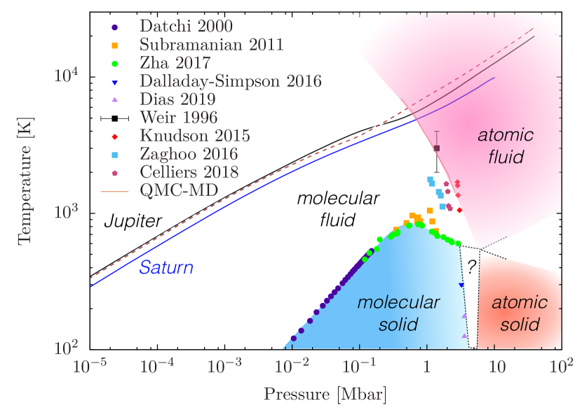
The availability of accurate measurements of the planets’ gravitational and magnetic fields requires the development of detailed structure models of the planets. The planetary internal structure is inferred from theoretical models that fit the available observational constraints by using theoretical EOSs for H, He, their mixtures, and the heavier elements. These models are guided by experiments and theoretical calculations of the thermodynamic properties of the relevant materials at high-pressure. Planetary interior models however, are non-unique and several of the assumptions made by the models rely on physical and chemical processes that are not fully understood (see section IV for discussion). Nevertheless, modeling giant planets in not possible without having a reliable EOS for H. Since laboratory experiments cannot cover the entire phase diagram for all relevant compositions, especially at extreme conditions (see section II.1), they need to be accompanied and complemented by theoretical calculations of the strongly interacting quantum systems of electrons and ions. Numerical simulations solve the corresponding N-particle Schrödinger equation using techniques like quantum Monte Carlo (QMC) or Density Functional Theory (DFT) simulations as discussed in section II.2. Figure 1 shows the hydrogen phase diagram in the typical ranges of pressure and temperature relevant for the giant planets.
This review provides an overview of the EOS of hydrogen, and hydrogen-helium EOS at planetary conditions, and the link between planetary interiors and high-pressure physics. In section II, we survey the progress in the experimental and theoretical/numerical fronts. In section III we discuss the behavior of hydrogen and a hydrogen-helium mixture at planetary conditions. Section IV briefly discusses how planetary interiors are models, focusing on Jupiter and Saturn. The current challenges and future are summarized in section V.
II Hydrogen
Compressed H is a system that has attracted the attention of both the theory and experimental communities for almost a century. Solid H has been predicted to metallize wigner , a fate shared with every other material under high enough compression, and to be a room-temperature superconductor PhysRevLett.21.1748 , with a speculated phase transition into a super-fluid phase, driven by proton quantum effects babaev2004superconductor . Below we review the continuing experimental and theoretical efforts, focusing on breakthroughs of the last five years; earlier work is summarized in mcmahon_properties_2012 . We then discuss the current consensus and open questions regarding the physics of dense liquid H.
II.1 Experiments
Static compression setups using DACs allow for a precise control of the temperature, compared to their dynamic counterpart, since the samples can be either cryogenically cooled PhysRevLett.75.2514 ; Diaseaal1579 , and resistively datchi2000extended or laser heated PhysRevLett.100.155701 ; dzyabura2013evidence ; zaghoo2016evidence ; zaghoo2017conductivity . While double-stage DACs can generally sustain record high pressures of GPa for metals dubrovinsky2015most , the high reactivity of dense H with the diamond limits the present achievable pressure at around GPa. Recently, Dias & Silvera Diaseaal1579 found evidence for solid metallic hydrogen in their experiments at 495 GPa. The highest conclusive pressure reached so far was 425 GPa loubeyre2020synchrotron . Further discussions on the validity of this result can be found in Goncharoveaam9736 ; Liueaan2286 ; commentloubeyre ; eremets1702comments ; geng2018public ; Silveraeaan1215 ; 2017arXiv170303064S . Several groups have been recently achieved pressures exceeding 300 GPa at T below 300 K. Such experiments revealed a very complex solid phase diagram featuring both temperature-driven howie2015raman and pressure-driven transition to novel solid non-metallic phases such as phase V dalladay2016evidence ; eremets2016low as well as phase -PRE dias2019quantum .
To summarize, standard DACs have conclusively reached pressures of 425 GPa at room temperature and reveal at least five solid phases dalladay2016evidence ; eremets2019semimetallic ; loubeyre2020synchrotron ; Gregoryanz2020 It remains inconclusive whether a metallic solid state has been reached Dias2017 ; Goncharoveaam9736 ; Liueaan2286 ; commentloubeyre ; eremets1702comments ; geng2018public ; Silveraeaan1215 ; 2017arXiv170303064S with recent experiments suggesting rather a semimetallic stateeremets2019semimetallic . Due to issues relating to sample containment, high temperature studies in static experiments are challenging with few experimental diagnostics that can conclusively determine either melting or conductivity.
Matter at extreme conditions has also been generated with dynamic compression techniques using shock waves 2017umdc.book…..N ; Nellis2019 . Modern experimental setups use, e.g., (i) impact of flyer plates accelerated to velocities as large as 8 or 45 km/s generated with a two-stage light gas gun weir1996metallization or pulsed power knudson2015direct , respectively, (ii) high-energy optical lasers Celliers677 , and (iii) spherical implosions driven by high explosives Mochalov2018 .
Experiments on pure H and pure He were recently presented using a combination of both methods, i.e. DACs to pre-compress the sample and then laser-driven shocks to further compress the material. The inferred data for both materials were obtained at much higher pressure conditions than on the cryogenic sample 2015JAP…118s5901B .
Recent advances in static compression experiments using DACs have paved the way to reach even higher temperatures and pressures so that the thermodynamic properties accessible for the two techniques will overlap in the future, and therefore can be used for benchmarking.
For decades dynamic-compression experiments were performed with sharp single-step shock waves. The conservation laws of mass, momentum, and energy restrict the thermodynamic path that can be reached for given starting initial conditions of the sample to so called Hugoniot curve defined by
| (1) |
where , , , , are internal energy, pressure, density, and temperature, respectively, and indicates the initial state. In dynamic compression experiments, , (the volume) and are generally determined by measurements of the velocities of the moving plate and by shock-impedance matching 2017umdc.book…..N ; Nellis2019 . This fact is of crucial significance because velocities are readily determined and thermodynamic states , , and cannot be determined directly at high pressures. While the thermodynamic relation computed through Eq. 1 remains the sole source of absolute EOS data at pressures above 5 Mbar, dynamic compression experiments also face challenges. Usually, determining the density has an uncertainty linked to the interferometric velocity measurement. A direct measurement of temperature is challenging, e.g., via streaked optical pyrometry (SOP) SOP , and is therefore often calculated from the spectrum of the emitted radiation, or estimated from theoretical models.
Given the limited range of pressure-temperature (-) that can be explored with this technique, the key of the Hugoniot data is to benchmark EOSs inferred from empirical models or first-principles simulations. The most accurate dynamical compression experiment with D reported by Knudson & Desjarlais PhysRevLett.118.035501 using pulsed power is affected with an error of only in density which allows to discriminate among various theoretical models. A similar accuracy has been obtained earlier using the same technique for water Knudson2012 . Nevertheless, other shock-compression techniques exhibit larger uncertainties so that a first-principles EOS for H valid for a wide range of and conditions as occurring in gas giants is rewarding.
In order to explore a larger portion of the thermodynamic space, and to reach higher densities while keeping the temperature relatively small, dynamical compression featuring multiple shocks or ramp compression techniques are now being used. The most recent experimental setups to study metallization of liquid H knudson2015direct ; Celliers677 , and high-pressure phases of water-ice millot2019nanosecond employ shock reverberation techniques.
The solid-liquid boundary can be assessed either via direct sample observation PhysRevLett.100.155701 ,
by tracing the plateau in the temperature versus laser heating curve PhysRevLett.100.155701 (latent heat), or from the disappearance of the Raman-active lattice modes eremets2009evidence ; Subramanian6014 ; PhysRevLett.119.075302 . Currently, the validity of both methods stated has been questioned by other research groups and should be further explored.
Nevertheless, all recent experiments agree on the presence of a maximum in the melting line at about 100 GPa, and the liquid phase is always found to be stable above K zha_high-pressure_2013 ; howie2015raman .
This finding rules out the existence of compressed solid molecular hydrogen in the deep interior of giant planets.
However, liquid H at planetary conditions undergoes
molecular dissociation and metallization.
Resistivity has been also directly measured using metal electrodes, in the pioneering work of Weir et al. weir1996metallization .
A large uncertainty in the measurement of the optical properties also leads to an uncertainty in the estimated metallisation pressure (100 GPa), which is typically defined as the pressure at which the conductivity of the system reaches the minimum metallic value of 2000 S/cm as introduced by Mott Mott1961 for K.
Different experimental studies aimed at identifying these transitions by searching for possibly abrupt changes in several properties of the samples. This is, however, an indirect way the characterise the transition, whose mechanism has to be interpreted from the data.
Since discontinuous changes in density, fingerprint of a first-order phase transition, are not observable in a fixed-volume DAC device, a phase transition in the liquid has been claimed from heating plateaus in static compression experiment dzyabura2013evidence ; ohta2015phase ; zaghoo2016evidence . This information alone is insufficient to assess metallization.
Electrical conductivity can be estimated from reflectivity and the absorption coefficient in both static zaghoo2017conductivity and dynamic compression experiments Celliers677 ; knudson2015direct ; zaghoo2017conductivity .
II.2 Numerical Calculations
Nowadays computer simulations are essential to understand fundamental physical problems and assist the experimental realization of novel materials. In the case of H at high pressure, computer studies also assist and complement experiments in understanding its rich phase diagram. Unlike experiments, in simulations one can monitor the ionic structures produced, and therefore, it is fairly straightforward, within the approximation of choice, to compute the relevant structures, the corresponding EOS, and the phase diagram.
Before the availability of powerful computers, the planetary physics community relied on semi-empirical models, employing classical force-fields fitted against available experimental data ross1983equation . A very successful semi-empirical EOS for H and He that covers a large range of temperatures and pressures is Saumon-Chabrier-Van Horn (SCVH) saumon1995equation , which qualitatively reproduces several liquid-phase experimental data from low- to high- pressure. This widely-used EOS in astrophysics which includes H, He and their mixture, has been recently updated 2019ApJ…872…51C and is in good agreement with existing experimental data and numerical simulations. Other frequently used EOS are those of Ross PhysRevB.58.669 and Kerley kerley2003 . Modern EOS tables are inferred from ab initio simulations using Density Functional Theory (DFT) in the warm dense matter regime (see below), rather than from experiments. The most recent versions are from the early 2010’s, by Caillabet et al. PhysRevB.83.094101 , Militzer and collaborators militzer2013ab ; 2013PhRvB..87a4202M and Becker et al. becker2014ab .
Indeed, the quantum mechanical treatment of the constituents, electrons, and protons is required. First-principles calculations are essential to model the interesting regime of pressures between 10 and 1000 GPa, and temperatures below K. These temperatures are sufficiently low that electrons cannot be modeled as an uniformly distributed background, and the system cannot be described by a two-component plasma brush1966monte . The dissociation and metallization transitions occur at pressures and temperatures of the order of 100 GPa and 1000 K, respectively, and the effects of electron correlations and their interactions in a non-uniform ionic lattice are particularly complex, and therefore very accurate electronic structure solvers are needed. Another source of complexity is linked to the protonic quantum effects that must be included at 1000-2000 K, and the protons cannot be treated as classical point-like particles morales_nuclear_2013 .
The commonly-used method to simulate materials at below - K is ab initio molecular dynamics (AIMD), which is basically an iterative scheme allen_computer_1987 involving the alternate solution of the Newton (for the nuclei, if treated classically) and the non-relativistic Schrödinger (for the electrons) equations. A notable exception, relevant for hydrogen, is the Coupled Electron-Ion Monte Carlo (CEIMC) method pierleoni_coupled_2004 , where ionic displacements do not follow the equation of motions, but are determined via Monte Carlo sampling.
Ab initio molecular dynamics is based on the Born-Oppenheimer approximation that decouples the ionic and electronic degrees of freedom RevModPhys.64.1045 ; alavi2009ab . The electronic structure is computed (approximately) at fixed ionic positions, then the nuclei are moved according to the forces, evaluated from the electronic ground state. This is a second approximation, called ground-state Born-Oppenheimer, which is valid in the range of temperatures considered. The accuracy of the forces depends on the degree of precision employed to solve the electronic problem. Thermo-states or baro-states are applied on the ionic degrees of freedom to sample from the desired constant-temperature (NVT), or constant-pressure (NPT) ensemble (see, e.g., andersen1980molecular ; allen_computer_1987 ; martyna1994constant ; bussi2007canonical ). Zero point motion of the nuclei, due to their quantum nature, can be included in a straightforward manner using path-integral methods PhysRevB.36.2092 ; cao1994formulation ; ceperley1995path ; morales_nuclear_2013 ; pierleoni2016liquid . The foundation of the AIMD method began with the pioneering work of Car & Parrinello PhysRevLett.55.2471 in 1985, where for the first time, a first-principles electronic structure calculation such as Density Functional Theory (DFT) hohenberg_inhomogeneous_1964 ; kohn_self-consistent_1965 was combined with molecular dynamics.
Density Functional Theory aims to solve the -particle Schrödinger equation via the exact electronic density instead of the many-body wavefunction. This method leads formally to the exact result, but the explicit functional introduced in the Kohn-Sham equations to describe exchange and correlation (XC) effects between electrons is unknown kohn_self-consistent_1965 . This key problem of DFT is subject of intensive work which has led to successively improved approximations burke_perspective_2012 . AIMD simulation results must be compared to available experimental data in order to benchmark their accuracy. Here we restrict the discussion to XC functionals that have been successfully used for H (see cohen2011challenges ; burke_perspective_2012 for details on the success and challenges of DFT). The Perdew-Burke-Ernzerhof (PBE) pbe XC functional has been chosen for the first simulations of the dense liquid, starting from the pioneering work of Scandolo scandolo2003liquid to more recent work lorenzen ; PhysRevB.75.024206 ; tamblyn2010structure ; morales_evidence_2010 , and solid H bonev2004quantum ; pickard2007structure ; liu2012room ; PhysRevB.87.174110 ; PhysRevB.85.214114 ; naumov2015chemical ; PhysRevLett.120.255701 . H-He mixtures have been studied with PBE as well Morales03022009 ; PhysRevLett.102.115701 . While PBE is still used, other and more sophisticated XC approximations have also been presented such as the Becke-Lee-Yang-Parr (BLYP) approximation blyp used in Refs. PhysRevLett.122.135501 ; PhysRevB.94.134101 , the HSE functional heyd2003hybrid , that is an approximation affected by a smaller self-interaction error, in Refs. PhysRevLett.122.135501 ; morales_nuclear_2013 , and functionals that include van-der-Waals long range interactions, such as vdw-DF1 vdwdf1 and vdw-DF2 vdwdf2 , in Refs. morales_nuclear_2013 ; knudson2015direct ; azadi2017role .
The performance of first-principles simulations has been checked against the most accurate Hugoniot data observed so far at Sandia’s Z machine PhysRevLett.118.035501 . The experimental data for the dissociation region are in disagreement with recent QMC calculations and better described by DFT simulations. However, none of the XC functionals is able to describe the complete experimental data set, but the vdW-DF1 functional seems to perform best. This finding has been confirmed recently by Knudson et al. Knudson2018 in re-analyzing the pioneering multiple shock wave experiments of Weir et al. weir1996metallization . Figure 2 presents Hugoniot curves (Eq. 1) for H and obtained when using different theoretical EOSs and compared with the experimental data.
Predictions of different XC functionals differ by up to 100-200 GPa concerning phase boundaries in the solid azadi_fate_2013 , and in the liquid morales_nuclear_2013 ; knudson2015direct . Calculated reflectivities and conductivities vary by about a factor of three across this range of approximations, and the EOS by morales_nuclear_2013 . Due to the lack of experimental data in the relevant - range, the performance of XC functionals can only be benchmarked against first-principles theories such as QMC-based methods. Recently a consensus has emerged that the vdw-DF1 vdwdf1 is the best performing approximation in both the liquid mazzola2018 ; pierleoni2016liquid , and solid phases PhysRevB.89.184106 , and is therefore the most commonly used DFT method in recent studies of H-He demixing PhysRevLett.120.115703 and optical properties across the dissociation rillo2019optical .
Electronic Quantum Monte Carlo is a wave-function-based method foulkes_quantum_2001 (unlike DFT), and is emerging as an accurate solver for electronic problems thanks to new generations of supercomputers. The main advantages of QMC compared to DFT are: (i) QMC relies on a many-body theory with a natural and explicit description of electron correlations, therefore the accuracy of calculations is in principle systematically improvable. (ii) QMC gives accurate results exhibiting, at the same time, a comparable scaling of computational cost with system size with DFT (although usually with a much larger prefactor). (iv) QMC is in an excellent position to take advantage of current and future supercomputer architectures, which are suitable for intrinsically parallel techniques.
Nevertheless, QMC algorithms are still more computationally expensive than DFT, and as a result, they have been traditionally used for benchmarking purposes PhysRevB.89.184106 ; clay2016benchmarking , or to assess relative stability between a limited number of candidate solid structures chen2014room ; PhysRevLett.112.165501 ; drummond2015quantum ; azadi2018nuclear . The simulation of liquids is significantly more challenging since the QMC electronic solver needs to be coupled with an efficient sampling method for the ions. To date, two different strategies have been established: the first uses QMC in a molecular dynamics fashion (QMC-MD) attaccalite_stable_2008 ; mazzola_unexpectedly_2014 ; mazzola_finite-temperature_2012 ; zen2015ab ; mazzola2017 ; mazzola2018 , and the second, CEIMC, employs a multilevel sampling approach for both electrons and ions pierleoni_coupled_2004 ; PhysRevLett.97.235702 ; morales_evidence_2010 ; morales2010eos ; PhysRevLett.115.045301 ; pierleoni2016liquid .
The QMC-MD approach is potentially indicated for the simulation of large systems, as it does not rely on the computation of energy differences, that are extensive quantities, at the cost of introducing an integration time step error attaccalite_stable_2008 . This approach has been employed for simulating other elements than H, such as water luo2014ab ; zen2015ab , and H-He mixtures mazzola2018 . The CEIMC method features a more sophisticated projective QMC solver, and can therefore achieve more accurate energetics. These two methods have been mainly used to simulate H dissociation and the metallization transition, and after some disagreements, they are now very consistent in predicting the nature and location of the dissociative transition in the liquid pierleoni2016liquid ; mazzola2018 . Hydrogen metallisation using QMC has been assessed either from direct conductivity calculationslin2009electrical or from ground-state properties mazzola2015distinct ; pierleoni2016liquid .
Nuclear quantum effects can be included in simulations using the path-integral formalism. In short, one point-like ion (with a classical representation) is replaced by a ring-polymer whose beads are interacting with suitable harmonic forcesmcmahon_properties_2012 . The configuration of this extended space can be sampled with MD or with Monte Carlo methods, where the forces associated with the electronic structure can be also computed at the DFT levelmorales_nuclear_2013 . Including nuclear quantum effects is essential for predicting the solid phasesmcmahon_properties_2012 , and for an accurate determination of the first-order transitionmorales_evidence_2010 ; knudson2015direct ; pierleoni2016liquid ; zaghoo2018striking . Table 1 lists the different computational methods and list their main strengths and weaknesses.
| Chemical models | Density Functional Theory | Quantum Monte Carlo | |
| Type | semi-empirical | first-principles | first-principles |
| Target | ionic force-fields | electronic density | electronic wavefunction |
| Strengths | covers a large range | a robust method | a nearly exact method |
| providing thermodynamical properties | large electrons number | identifies well phase transitions | |
| Weaknesses | non first-principle, not exact | not exact, results depend on XC functionals | hard to benchmark, computationally expensive |
| based on effective potentials | computationally expensive | small electrons number | |
| Simulation size | — | up to electrons | electrons |
III H and H-He at planetary conditions
III.1 Pure hydrogen
At temperatures of a few thousand Kelvin, relevant for the deep interiors of Jupiter and Saturn, the dissociation and metallization transition of pure-H is a continuous process. The most recent experiments performed at these conditions are reported by Davis et al. davis2016x , where x-ray scattering measurements in dynamically compressed deuterium shows an onset of ionization at around 20-40 GPa and 3500-4500 K, and by McWilliams et al. PhysRevLett.116.255501 who found a continuous transition at these conditions. This picture is compatible with DFT tamblyn2010structure ; morales_evidence_2010 and QMC simulations pierleoni2016liquid ; mazzola2018 , which all report continuous transitions above 2000-3000 K. Most of the recent experiments and simulations provide evidences for of a first-order transition up to 1200-1500 K zaghoo2016evidence ; knudson2015direct ; ohta2015phase ; morales_evidence_2010 ; lorenzen ; pierleoni2016liquid ; mazzola2018 . Nevertheless, a quantitative agreement on the location of the phase boundary, as well as a precise (within accuracy) determination of the EOS for pure-H, is still missing. Traditionally, the principal single-shock Huguniot has been identified as the benchmark for simulations. Interestingly, even when considering the experimental uncertainty discussed in Sect. II.1, EOSs obtained with DFT are in better agreement with experiments compared to the QMC data, computed using CEIMC PhysRevLett.115.045301 . Recently, Clay et al. PhysRevB.100.075103 suggested that this behavior can be explained by a more favourable error cancellation in the variables , , entering the Rankine-Huguniot equation.
We therefore suggest that the available EOSs for hydrogen should be benchmarked with the -- relations computed with the most recent QMC calculations by Pierleoni et al. pierleoni2016liquid (CEIMC) and Mazzola et al. mazzola2018 (QMC-MD). While a QMC-EOS table for a wide - regime is still missing, the - relation at K computed in Ref. mazzola2018 reveals a denser EOS by about , compared to the current DFT-PBE based ones militzer2013ab ; becker2014ab .
State-of-the-art ab-initio setups feature simulation cells consisting of up to 512 (128) particles at the DFT (QMC) level of theory for production runs lorenzen ; Geng2019 . Electronic finite size effects errors are mitigated by Brillouine zone sampling PhysRevLett.102.115701 ; holzmann2016theory ; Geng2019 . This setup can provide satisfactory accuracy in the liquid phase. However, this can change in the solid phase and generally near phase transitions, where insufficient equilibration times or too small sizes can artificially stabilise one competing phase against another, e.g., delaying the onset of metallization, or hindering the possibility to distinguish a first-order from a continuous transition. In hydrogen this issue is amplified because the melting line and the dissociation transition between the molecular and the atomic liquid lie quite close in the phase diagram.
Simulating very large ensembles particles with AIMD is not yet possible so that studies on mixtures is limited (e.g. miscibility of water soubiran2015miscibility , iron soubiran2015miscibility , and MgO PhysRevLett.108.111101 , or decomposition of hydrocarbons ancilotto1997dissociation in hydrogen), especially when we need to establish possible phase separation of low stoichiometry heavy elements (e.g. mixtures to simulate the composition of the ice giant planets Uranus and Neptune chau2011chemical ). Novel methods such as stochastic DFT Cytter2019 or machine-learning based investigation are expected to bridge this gap in future simulations G2019 .
III.2 Hydrogen and helium mixture
Despite its importance, there are very scarce experimental data concerning the phase diagram of H-He mixtures, which are still limited to room temperature PhysRevB.36.3723 ; loubeyre1991new ; PhysRevLett.120.165301 ; 2018PhRvL.121s5702T . H-He mixtures have been predicted to undergo a (temperature-driven) transition from a high-T fully miscible liquid, to a low-T phase-separated with helium-rich droplets 1977ApJS…35..239S ; 1977ApJS…35..221S ; mcmahon_properties_2012 . Therefore, the interaction between H and He under the interior conditions of Jupiter and Saturn leads to challenges in determining the EOS of mixture due to the expected immiscibility of He in H, results in He settling (”helium rain”). This process, is expected to impact the planetary structure as we discuss in more detail in Sect. IV.
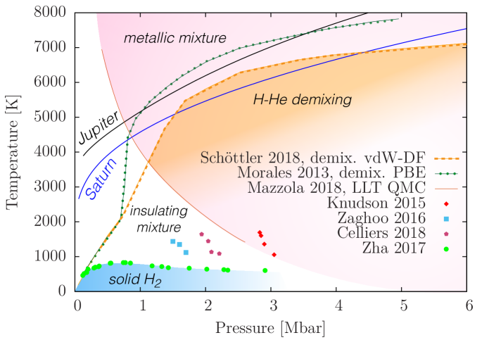
The existing knowledge on the liquid phase and H-He demixing is based on simulations. Most recent studies employ DFT at the PBE level, computing the free-energy under the ideal-mixing approximation for the entropy of mixing PhysRevLett.102.115701 , and under the non-ideal one morales2009phase . The latter reference is obtained with thermodynamic integration and is expected to be more accurate, with a shift (toward low-T) of the demixing temperature of order of 1000 K. This computation was recently revisited using the more accurate vdw-DF functional and non-ideal entropy of mixing by Schöttler & Redmer PhysRevLett.120.115703 who found lower demixing temperatures, slightly below the Jupiter adiabat (black solid) and crossing that of Saturn (black dashed) between 1.5 and 4 Mbar as shown in Figure 3. A change of optical properties upon demixing of H and He was predicted by Soubrian et al. 2013PhRvB..87p5114S and is expected to be tested by experiments in the near future.
Phase separation is not the only important physical process that distinguish H-He mixtures from pure hydrogen. The presence of helium stabilizes the hydrogen molecules, delaying the onset of metallization towards higher densities. Such a shift has been calculated with QMC by Mazzola et al. mazzola2018 : it amounts GPa at 1500 K and GPa at 6000 K. Therefore, the continuous transition from molecular to metallic H-He mixture in Jupiter’s conditions is expected to occur between 40 and 60 GPa mazzola2018 .
IV Modeling Planetary Interiors
Traditionally Jupiter and Saturn were viewed as laboratories for understanding the EOS, however, as our knowledge has grown the importance of other complexities have arisen as we discuss below. Planetary models aim to determine the internal structure of planets, i.e., the composition and its depth dependence. This is done by constructing interior models assuming various different structures and compositions that fit and reproduce the planetary observed properties such as the mass, radius, luminosity, and gravitational field data.
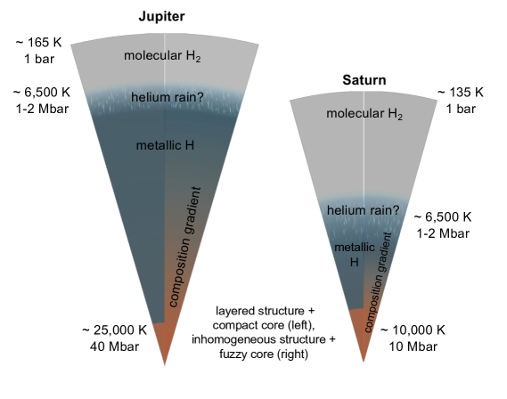
Jupiter and Saturn are often referred as ”gas giant planets”, however, the bulk of their interiors are in fact not in the gaseous phase due to the high pressures and temperatures as can be seen in Figure 1. As a result, Jupiter and Saturn are in fact ”fluid giant planets”. While in their low-P atmospheres H is in a molecular form, and the densities are low, the deep interiors of the planets are characterised by condensed (liquid) H, and therefore one should think of these planets as ”fluid planets”. It should also be noted that gas giant planets do not have a surface like in the case of terrestrial planets, and therefore there is no real transition between the planetary atmosphere and the deep interior. At the same time, there is no exact location where the atmosphere ends since the outer regions of the atmosphere are characterised by a very low-density gas. As a result, planetary scientists define the ”surface” of a gas giant planet at the location where the pressure is 1 bar, similar to the pressure on Earth’s surface. The temperature at this location is measured (with a small uncertainty). Then, with information of the temperature at 1 bar, the entropy of the outer envelope is determined and (adiabatic) models can be constructed guillot_interiors_2005 . The basic observed properties of Jupiter and Saturn are listed in Table 2. Recent review chapters about the giant planets can be found in Refs. FJ2016 ; MB2016 ; HG2018 ; RH2018 and references given therein.
The modelled planetary interior can consist of different layers, where the number of layers is often chosen to be the minimum number of layers (typically three) that is required to fit the observational data, and be consistent with our knowledge of the material properties. The main sources of uncertainty in interior models arise from the assumed number of layers, the assumed composition and its distribution, the heat transport mechanism, and the dynamical effects that are typically neglected or treated in a simplified manner. Another important source of uncertainty is the physics of dense hydrogen (and helium) and the understanding of the nature of the phase transitions in that determine the planetary density profile.
Planetary structure models are constructed assuming the planet is in hydrostatic equilibrium, and rely on conservation of mass and of momentum:
| (2) |
| (3) |
where is the mass within a sphere of a radius , is the pressure, is the density at , is the planetary rotation rate (typically assumed to be constant, i.e., uniform rotation) and is the gravitational constant. In order to infer the temperature profile within the planet the thermodynamic equation must be solved. The determination of the temperature profile, however, is not simple, and depends on the heat transport mechanism within the planet. This can be radiation, conduction, and convection, where the latter can also have more sophisticated versions such as layered-convection. relies on complex physics that is still being investigated (LC12, ; LC13, ; DC19, ; Vazan16, ; Vazan18, ).
For simplicity, for a few decades Jupiter and Saturn were assumed to be fully convective, so the temperature gradient was assumed to be the adiabatic gradient . Last but not least, in order to model the planetary internal structure knowledge of the density dependency on the temperature and pressure, i.e., is needed. This is essentially the knowledge of the EOS of the assumed materials. Since both Jupiter and Saturn consist of mostly H and He, modelling their internal structures requires knowledge of the behaviour of these materials for a wide range of pressures (1 bar up to few ten Mbar) and temperatures (165 K up to a few 10,000 K).
It should be mentioned that there is an alternative approach to model planetary interiors by constructing ”empirical models” 1995JGR…10023349M ; 2000P&SS…48..143P ; 2009Icar..199..368H ; 2011ApJ…726…15H . These models do not rely on a physical EOS, and instead, the density profile has a mathematical representation such as polynomials or polytropes. Then by assuming hydrostatic equilibrium the planetary - profile that reproduces the planetary observed parameters can be found. Although in such models the temperature profile cannot be determined, the composition can be inferred from the - relation combined with an assumed temperature gradient. The main advantage of this approach is that it is less biased by the modeller’s assumption, and it can lead to a larger parameter-space of solutions.
| Physical Property | Jupiter | Saturn |
|---|---|---|
| Distance to Sun (AU) | 5.204 | 9.582 |
| Mass (1024 kg) | 1898.130.19 | 568.3190.057 |
| Mean Radius (km) | 699116 | 582326 |
| Equatorial Radius (km) | 714924 | 602684 |
| Mean Density (g/cm3) | 1.32620.0004 | 0.68710.0002 |
| 14696.5720.014 | 16290.5730.028 | |
| -586.6090.004 | -935.3140.037 | |
| 34.1980.009 | 86.3400.087 | |
| Rotation Period | 9h 55m 29.56s | 10h 39m 10mii |
| Effective Temperature (K) | 124.40.3 | 95.00.4 |
| 1-bar Temperature (K) | 1654 | 1355 |
ithese are theoretical values based on interior model calculations. iisee FJ2016 and references therein for discussion on Saturn’s rotation rate uncertainty.
IV.1 Jupiter and Saturn
Revealing information on the deep interiors of Jupiter and Saturn must be done by using indirect measurements. Jupiter and Saturn are the most massive planets in the Solar System. The masses of Jupiter and Saturn are about 318 and 95 times the mass of Earth, respectively. Jupiter’s average radius is 69,911 km, more than ten times Earth’s radius. Saturn’s average radius is slightly smaller and measured to be 58,232 km (see Table 2 for details).
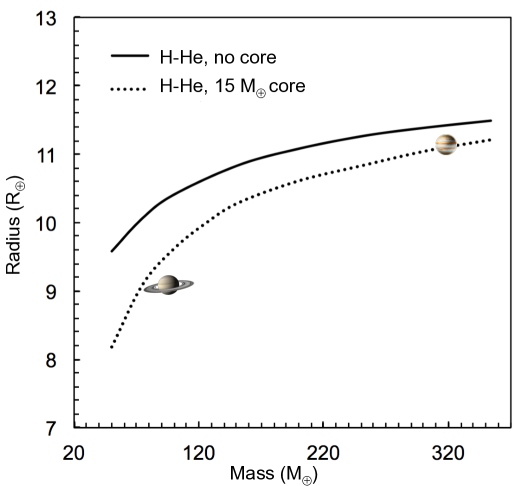
The relation between mass and radius provides information about the planet’s average density and therefore its bulk composition. The average densities of Jupiter and Saturn are 1.3262 g/cm3 and 0.687 g/cm3, respectively. The lower average density of Saturn is not a result of a more volatile composition, but due to the smaller effect of compression due to its smaller mass. Figure 4 shows a mass-radius (M-R) relation for H-He-rich planets with different compositions and the measured M-R relation of Jupiter and Saturn. It can be seen from the figure that both Jupiter and Saturn lie close to the H-He curves, suggesting that they consist of mostly H-He, but also have a fraction of heavy elements 2014arXiv1405.3752G . These heavier elements are typically assumed to be rocks (i.e., silicates and sometimes metals) and/or ices (H2O but also CH4 and NH3). In addition, since Saturn’s distance to the pure-H-He curve is larger than that of Jupiter, it is expected to be more enriched with heavy elements. Although understanding the internal structure of Jupiter and Saturn relies on the H, and H-He EOS, the heavier elements play key role in the formation and evolution of the planets (see 2014prpl.conf..643H ; HG2018 ; RH2018 and references therein).
In addition, there are several interesting conclusions about Jupiter and Saturn that can be made simply by plotting their inferred - profiles on to of the H phase diagram as shown in Figure 1. First, both planets lie in the regime above solid H, showing that they are indeed fluid planets. Second, both planets cross the metallization transition, which is continuous at these temperatures, indicating a smooth transition between molecular and non-to-semiconducting hydrogen in the outer parts of the planets () and conducting (or metallic) atomic hydrogen (H) in their deep interiors.
The H-He EOS data predetermine the - profiles of the planets. However, the corresponding material data such as compressibility and specific heat have a sensitive impact on the slope of these profiles. For instance, the fraction of heavy elements to be mixed with H-He in order to match the measured gravity data and the mass of the core depend on the stiffness of the H-He EOS. Therefore, uncertainties in the ab initio H-He EOS of as currently valid still have a rather big influence on interior models, and progress in ab initio simulations and in high-pressure experiments will directly lead to advanced interior models. However, an additional complexity as discussed below is linked to the heat transport mechanism within the planets which is not well determined, and therefore introduces an uncertainly in the planetary temperature profile. Finally, it is clear that Saturn’s P-T profile covers lower temperatures and pressures (due to its smaller mass which leads to smaller compression).
Since the high-P regime of the H EOS is less understood, interior models of Saturn suffer less from the uncertainty in the H EOS. This is, however, the opposite when it comes to H-He demixing as indicated by Figure 3. Since Saturn’s adiabat crosses the phase separation line is closer its internal structure is more affected by the phase separation of He. This leads to further complexity in modelling Saturn’s internal structure, and can also affect its energetics and long-term evolution 2003Icar..164..228F ; LC13 ; 2016ApJ…832..113M ; Vazan2016 ; 2016Icar..267..323P ; FJ2016 .
Traditionally, internal structure models of Jupiter and Saturn consisted of three distinct layers: a heavy-element core, an inner envelope of metallic hydrogen, and an outer envelope of molecular hydrogen. Due to helium separation, the He mass fraction was assumed to be enriched in the inner envelope and depleted in the outer one. The envelopes were also assumed to consist of heavier elements, and their distribution, which was assumed either to be uniformly mixed in both envelopes, or discontinuous across the two envelopes, was a free parameter in the models. These traditional models assumed that the temperature profile of the planet is given by the adiabatic gradient =, where is the entropy. This assumption, however, holds only for a planet which is homogeneous and fully convective. It is now clear that both Jupiter and Saturn have more complex interiors, including composition gradients and regions that are stable against convection where heat is transported by conduction or layered-convection 2019ApJ…872..100D ; DC19 ; Vazan18 ; Vazan2016 ; LC13 ; LC12 .
For Jupiter, accurate gravity data have become available thanks to the Juno mission 2017Sci…356..821B ; Iess2018 . This led to the development of new structure models, with the preferred solutions being ones with dilute cores and a discontinuity of the heavy-element enrichment in the envelope, with the inner He-rich envelope consists of more heavy elements than the outer, helium-poor envelope 2017GeoRL..44.4649W ; 2017A&A…606A.139N ; 2018Natur.555..227G ; DC19 . These Jupiter structure models that fit Juno data suggest that giant planets’s cores should not be viewed as compact regions consisting mostly of heavy elements but as central regions whose compositions are dominated by heavy elements, which could be gradually distributed or homogeneously mixed. A diluted core for Jupiter could extend to a few tens of percents of the planet’s total radius, and can also consist of lighter elements, and is actually consistent with the current view of the formation process of gas giant planets 2017ApJ…840L…4H . It should be noted that the inferred structure of the planets depends on the used EOS. Also the Cassini mission provided more accurate measurements of Saturn’s gravitational field that significantly improved in the last phase of the mission Iess2019 . Saturn structure models that fit Cassini data suggest that Saturn has a relatively massive core of about 15 Earth masses and that its envelope consist of only a few Earth masses of heavy elements 2019ApJ…879…78M , with the exact number depending on the assumed rotation period (which is uncertain within a few minutes), and other model parameters 2013ApJ…767..113H ; 2019GeoRL..46..616G . These new structure models clearly suggest that the temperature profiles in the planetary deep interior can significantly differ from the adiabatic one. This in return can affect the inferred heavy-element mass since hotter interiors lead to higher enrichment for a given density. As a result, improvements in planetary structure models do not only depend on the EOS of the pure materials, but on the more complex interplay of mixtures, phase separations, as well as other physical conditions and processes such as heat transport and convective and mixing efficiencies in the presence of composition gradients. Advances in giant planet modeling can also be improved using other data. For example, the splitting of the low order f-modes of Saturn’s oscillations Saturn confirms that the deep interior is non-homogeneous and consists of composition gradients2014Icar..242..283F . In Figure 3 we present the - profiles inferred from adiabatic and non-adiabatic models for comparison.
The much more accurate gravity data has led to the development of more complex structure models that include composition gradients and account for the dynamical contributions. Interestingly, the improvements in the quality of the gravity data led to many new questions regarding the planetary interiors, and standard structure models have been challenged. It is now clear that the internal structures of Jupiter and Saturn are complex, and are not only dependent on our understanding of the EOS dominating in these objects but also on the heat transport mechanism, the actually internal structure and composition, as well as the thermodynamics and chemistry operating in their deep interiors.
In addition, the two planets are different from each other, and the challenges in their modelling is not the same - while for Jupiter the largest uncertainty is linked to the H EOS, for Saturn it is the H-He phase diagram and the uncertainty in its rotation period. Figure 6 provides a schematic presentation of the two possible internal structures of Jupiter and Saturn, the traditional structure with three distinct layers, and one with composition gradients (see HG2018 ; 2018oeps.book..175H and references therein for further details).
IV.2 Planetary magnetic fields
The fact that Jupiter and Saturn have strong magnetic fields also provides important information on their composition and internal structure. In order to possess a magnetic field three criteria should be satisfied: (i) the planet must consist of a region of electrically conductive fluid, (ii) this region should be convective, and (iii) the planet should rotate (at least moderately) rapidly. The mechanism for magnetic field generation in planetary interior, also known as dynamo theory, is not well understood and is still being investigated. Dynamo generation is related to the physics of MHD and the interplay between fluid dynamics and electro-magnetism and is currently assessed via numerical simulations. More information on the connection between high-pressure physics, interior models, and dynamo simulations can be found in Lühr et al. 2018ASSL..448…..L .
Since both Jupiter and Saturn possess dipolar intrinsic magnetic fields, we can conclude that the material in their deep interior is electrically conducting and that at least in part of their interiors, heat is transported through convection.
Both planets rotate fast enough to generate a dynamo.
For Jupiter and Saturn, the conducting material is thought to be metallic hydrogen.
The strong connection between planetary interiors and high-pressure physics is therefore clear: from the mean densities of the gas giants can be concluded that they are H-dominated, and since that they possess magnetic fields, one can conclude that H metallises at such high pressures.
In both Jupiter and Saturn the electrical
conductivity increases significantly even before full metallization of H is reached French2012 .
The magnitude of the electrical conductivity inside the gas giants, combined with the planetary measured magnetic field strength and luminosity, can be used to estimate the internal Ohmic dissipation and introduce additional constraints for structure and dynamical models (e.g., Liu2008 ; Cao2017 ; 2014GeoRL..41.5410G ; 2014Icar..241..148J ; 2019A&A…629A.125W ; 2019ApJ…879L..22D ).
Jupiter’s magnetic field is the strongest in the Solar System (excluding the Sun), and its surface field strength is between 4 and 20 Gauss Connerney2018 ; Moore2018 .
Recently, the Juno spacecraft revealed that Jupiter’s magnetic field has an intense isolated magnetic spot near the equator with a negative flux.
In addition, an intense and relatively narrow band of positive flux near 45 degrees latitude in the northern hemisphere was found together with a rather smooth magnetic field in the southern hemisphere.
Also the north-south dichotomy in Jupiter’s magnetic field structure could be explained by the existence of a diluted core Moore2018 .
Saturn’s magnetic field which has a surface field strength of 0.2-0.5 Gauss (e.g., 2005Sci…307.1266D ; 2017AGUFM.U22A..02D ; 2019arXiv191106952C ) is nearly perfectly symmetric with respect to the spin-axis 2012Icar..221..388C .
The characteristic of Saturn’s magnetic field could be a result of He rain, which could create a stable (against convention) below/above the dynamo. A stable deep interior can also be a result of composition gradients and non-adiabatic interiors.
Understanding these processes and their outcomes requires good knowledge of the associated thermodynamics and the feedback on the magnetic field and vice versa.
While the current understanding of the dynamo process is still limited, and as a result, the magnetic fields can only be used to set some bounds on the material properties and heat transports inside the planets. This however, can change in the future.
V Challenges and Outlook
The ongoing progress in science leads to the solution of long-lasting open questions, and yet, new questions and challenges arise.
Although our understanding of the giant planets and the behaviour of elements at planetary conditions is still incomplete, we expect significant progress in the near future.
Upcoming experiments and theoretical models are expected to enhance our understanding of phase transitions, mixtures, and immiscibilities. We also foresee improvements in numerical calculations given the increasing computation power and the development of new numerical techniques.
In particular, we expect that future experiments will resolve the disagreement on the hydrogen metallization conditions and get consistent results using the various methods.
In addition, it would be desirable to make experiments of H-He mixtures in order to investigate the demixing of helium in hydrogen.
Another topic that is expected to blossom in the future is superconductivity. While superconductivity has yet to be found in pure H, the hypothesis of supercontactive H directed the search for superconductivity in H-rich materials drozdov2015conventional ; liu2017potential .
Finally, in this review we focused on Jupiter and Saturn and have not discussed the ice giants Uranus and Neptune.
The ice planets are key for understanding planet formation and for the characterisation of intermediate planets around other stars.
Since these planets are thought to consist of volatiles like water, methane, and ammonia and experimental data focusing on these materials would be valuable.
In addition, the influence of H-He on the mixtures of these materials and the role of carbon is yet to be determined.
We also expect progress in our understating of the internal structures
of Jupiter and Saturn given the ongoing efforts in the processing and the interpretation of recent data from the Juno and Cassini missions, and the development of more comprehensive structure models.
In addition, upcoming and future space missions will also play a key role in better constraining the interiors of the gas giants.
The planned ESA JUICE mission will reveal further information on Jupiter, and a potential Saturn probe mission will provide constraints on Saturn’s atmospheric composition and the immiscibility of He in H and the process of phase separation.
Nevertheless, it is now realized that giant planets interiors are much more complex than previously thought. As a result, to better understand giant planets improvements of the H and H-He EOS are required but insufficient. We suggest that future studies should concentrate on mixtures, phase transitions, and their physical properties such as thermal diffusivity, electrical conductivity, and opacity. These properties can then be used to further constrain giant planet formation, evolution, and structure models.
The link between planetary interiors and high-pressure physics is therefore clear, and we believe that the future holds great promises in this direction.
Acknowledgements
We thank the anonymous referees for valuable comments that helped to improve the manuscript. We also acknowledge support from W. Nellis, F. Soubrian, S. Sorella, D. Stevenson, N. Nettelmann, J. J. Fortney, Y. Miguel, S. Müller, C. Valletta, and A. Cumming. RH acknowledges support from SNSF grant 200020_188460 and thanks the Juno science-team members for inspiring discussions. RR acknowledges support by the DFG via the projects FOR 2440 and SPP 1992.
References
-
(1)
J. M. McMahon, M. A. Morales, C. Pierleoni, D. M. Ceperley,
The properties of
hydrogen and helium under extreme conditions, Reviews of Modern Physics
84 (4) (2012) 1607–1653.
doi:10.1103/RevModPhys.84.1607.
URL http://link.aps.org/doi/10.1103/RevModPhys.84.1607 -
(2)
E. Wigner, H. B. Huntington, On the
possibility of a metallic modification of hydrogen, The Journal of Chemical
Physics 3 (12) (1935) 764–770.
arXiv:http://dx.doi.org/10.1063/1.1749590, doi:10.1063/1.1749590.
URL http://dx.doi.org/10.1063/1.1749590 -
(3)
E. Gregoryanz, C. Ji, P. Dalladay-Simpson, B. Li, R. T. Howie, H.-K. Mao,
Everything you always wanted to know
about metallic hydrogen but were afraid to ask, Matter and Radiation at
Extremes 5 (3) (2020) 038101.
arXiv:https://doi.org/10.1063/5.0002104, doi:10.1063/5.0002104.
URL https://doi.org/10.1063/5.0002104 - (4) S. Weir, A. Mitchell, W. Nellis, Metallization of fluid molecular hydrogen at 140 gpa (1.4 mbar), Physical Review Letters 76 (11) (1996) 1860.
- (5) R. Helled, J. D. Anderson, M. Podolak, G. Schubert, Interior Models of Uranus and Neptune, ApJ 726 (1) (2011) 15. arXiv:1010.5546, doi:10.1088/0004-637X/726/1/15.
- (6) F. Datchi, P. Loubeyre, R. LeToullec, Extended and accurate determination of the melting curves of argon, helium, ice (h 2 o), and hydrogen (h 2), Physical Review B 61 (10) (2000) 6535.
-
(7)
N. Subramanian, A. F. Goncharov, V. V. Struzhkin, M. Somayazulu, R. J. Hemley,
Bonding changes in hot fluid
hydrogen at megabar pressures, Proceedings of the National Academy of
Sciences 108 (15) (2011) 6014–6019.
arXiv:https://www.pnas.org/content/108/15/6014.full.pdf, doi:10.1073/pnas.1102760108.
URL https://www.pnas.org/content/108/15/6014 -
(8)
C.-s. Zha, H. Liu, J. S. Tse, R. J. Hemley,
Melting and
high transitions of hydrogen up to 300 gpa, Phys.
Rev. Lett. 119 (2017) 075302.
doi:10.1103/PhysRevLett.119.075302.
URL https://link.aps.org/doi/10.1103/PhysRevLett.119.075302 - (9) P. Dalladay-Simpson, R. T. Howie, E. Gregoryanz, Evidence for a new phase of dense hydrogen above 325 gigapascals, Nature 529 (7584) (2016) 63.
- (10) R. P. Dias, O. Noked, I. F. Silvera, Quantum phase transition in solid hydrogen at high pressure, Physical Review B 100 (18) (2019) 184112.
- (11) M. Knudson, M. Desjarlais, A. Becker, R. Lemke, K. Cochrane, M. Savage, D. Bliss, T. Mattsson, R. Redmer, Direct observation of an abrupt insulator-to-metal transition in dense liquid deuterium, Science 348 (6242) (2015) 1455–1460.
- (12) M. Zaghoo, A. Salamat, I. F. Silvera, Evidence of a first-order phase transition to metallic hydrogen, Physical Review B 93 (15) (2016) 155128.
-
(13)
P. M. Celliers, M. Millot, S. Brygoo, R. S. McWilliams, D. E. Fratanduono,
J. R. Rygg, A. F. Goncharov, P. Loubeyre, J. H. Eggert, J. L. Peterson, N. B.
Meezan, S. Le Pape, G. W. Collins, R. Jeanloz, R. J. Hemley,
Insulator-metal
transition in dense fluid deuterium, Science 361 (6403) (2018) 677–682.
arXiv:http://science.sciencemag.org/content/361/6403/677.full.pdf,
doi:10.1126/science.aat0970.
URL http://science.sciencemag.org/content/361/6403/677 -
(14)
G. Mazzola, R. Helled, S. Sorella,
Phase diagram
of hydrogen and a hydrogen-helium mixture at planetary conditions by quantum
monte carlo simulations, Phys. Rev. Lett. 120 (2018) 025701.
doi:10.1103/PhysRevLett.120.025701.
URL https://link.aps.org/doi/10.1103/PhysRevLett.120.025701 - (15) R. Helled, The Interiors of Jupiter and Saturn, 2018, p. 175. doi:10.1093/acrefore/9780190647926.013.175.
- (16) F. Debras, G. Chabrier, New Models of Jupiter in the Context of Juno and Galileo, Astrophys. J. 872 (1) (2019) 100. arXiv:1901.05697, doi:10.3847/1538-4357/aaff65.
-
(17)
N. W. Ashcroft,
Metallic
hydrogen: A high-temperature superconductor?, Phys. Rev. Lett. 21 (1968)
1748–1749.
doi:10.1103/PhysRevLett.21.1748.
URL https://link.aps.org/doi/10.1103/PhysRevLett.21.1748 - (18) E. Babaev, A. Sudbø, N. Ashcroft, A superconductor to superfluid phase transition in liquid metallic hydrogen, Nature 431 (7009) (2004) 666.
-
(19)
A. F. Goncharov, I. I. Mazin, J. H. Eggert, R. J. Hemley, H.-k. Mao,
Invariant points
and phase transitions in deuterium at megabar pressures, Phys. Rev. Lett. 75
(1995) 2514–2517.
doi:10.1103/PhysRevLett.75.2514.
URL https://link.aps.org/doi/10.1103/PhysRevLett.75.2514 -
(20)
R. P. Dias, I. F. Silvera,
Observation
of the wigner-huntington transition to metallic hydrogen, Science (2017).
arXiv:http://science.sciencemag.org/content/early/2017/01/25/science.aal1579.full.pdf,
doi:10.1126/science.aal1579.
URL http://science.sciencemag.org/content/early/2017/01/25/science.aal1579 -
(21)
S. Deemyad, I. F. Silvera,
Melting line
of hydrogen at high pressures, Phys. Rev. Lett. 100 (2008) 155701.
doi:10.1103/PhysRevLett.100.155701.
URL https://link.aps.org/doi/10.1103/PhysRevLett.100.155701 - (22) V. Dzyabura, M. Zaghoo, I. F. Silvera, Evidence of a liquid–liquid phase transition in hot dense hydrogen, Proceedings of the National Academy of Sciences 110 (20) (2013) 8040–8044.
- (23) M. Zaghoo, I. F. Silvera, Conductivity and dissociation in liquid metallic hydrogen and implications for planetary interiors, Proceedings of the National Academy of Sciences (2017) 201707918.
- (24) L. Dubrovinsky, N. Dubrovinskaia, E. Bykova, M. Bykov, V. Prakapenka, C. Prescher, K. Glazyrin, H.-P. Liermann, M. Hanfland, M. Ekholm, et al., The most incompressible metal osmium at static pressures above 750 gigapascals, Nature 525 (7568) (2015) 226.
- (25) P. Loubeyre, F. Occelli, P. Dumas, Synchrotron infrared spectroscopic evidence of the probable transition to metal hydrogen, Nature 577 (7792) (2020) 631–635.
-
(26)
A. F. Goncharov, V. V. Struzhkin,
Comment on
“observation of the wigner-huntington transition to
metallic hydrogen”, Science 357 (6353) (2017).
arXiv:http://science.sciencemag.org/content/357/6353/eaam9736.full.pdf,
doi:10.1126/science.aam9736.
URL http://science.sciencemag.org/content/357/6353/eaam9736 -
(27)
X.-D. Liu, P. Dalladay-Simpson, R. T. Howie, B. Li, E. Gregoryanz,
Comment on
“observation of the wigner-huntington transition to
metallic hydrogen”, Science 357 (6353) (2017).
arXiv:http://science.sciencemag.org/content/357/6353/eaan2286.full.pdf,
doi:10.1126/science.aan2286.
URL http://science.sciencemag.org/content/357/6353/eaan2286 - (28) P. Loubeyre, F. Occelli, P. Dumas, Comment on: Observation of the Wigner-Huntington transition to metallic hydrogen, arXiv e-prints (2017) arXiv:1702.07192arXiv:1702.07192.
- (29) M. Eremets, A. Drozdov, Comments on the claimed observation of the wigner-huntington transition to metallic hydrogen, 2017, arXiv preprint arXiv:1702.05125.
- (30) H. Y. Geng, Public debate on metallic hydrogen to boost high pressure research, Matter and Radiation at Extremes 2 (6) (2018) 275.
-
(31)
I. Silvera, R. Dias,
Response to
comment on “observation of the wigner-huntington transition
to metallic hydrogen”, Science 357 (6353) (2017).
arXiv:https://science.sciencemag.org/content/357/6353/eaan1215.full.pdf,
doi:10.1126/science.aan1215.
URL https://science.sciencemag.org/content/357/6353/eaan1215 - (32) I. Silvera, R. Dias, Response to critiques on Observation of the Wigner-Huntington transition to metallic hydrogen, arXiv e-prints (2017) arXiv:1703.03064arXiv:1703.03064.
- (33) R. T. Howie, P. Dalladay-Simpson, E. Gregoryanz, Raman spectroscopy of hot hydrogen above 200 gpa, Nature materials 14 (5) (2015) 495–499.
- (34) M. Eremets, I. Troyan, A. Drozdov, Low temperature phase diagram of hydrogen at pressures up to 380 gpa. a possible metallic phase at 360 gpa and 200 k, arXiv preprint arXiv:1601.04479 (2016).
- (35) M. I. Eremets, A. P. Drozdov, P. Kong, H. Wang, Semimetallic molecular hydrogen at pressure above 350 gpa, Nature Physics 15 (12) (2019) 1246–1249.
-
(36)
R. P. Dias, I. F. Silvera,
Observation of the
wigner-huntington transition to metallic hydrogen, Science 355 (6326) (2017)
715–718.
arXiv:https://science.sciencemag.org/content/355/6326/715.full.pdf,
doi:10.1126/science.aal1579.
URL https://science.sciencemag.org/content/355/6326/715 - (37) W. Nellis, Ultracondensed Matter by Dynamic Compression, 2017.
- (38) W. J. Nellis, Dense quantum hydrogen, Low Temperature Physics 45 (3) (2019) 294–296. doi:10.1063/1.5090043.
- (39) M. A. Mochalov, R. I. Il’kaev, V. E. Fortov, A. L. Mikhailov, V. A. Arinin, A. O. Blikov, V. A. Komrakov, I. P. Maksimkin, V. A. Ogorodnikov, A. V. Ryzhkov, Quasi-Isentropic Compressibility of Deuterium at a Pressure of 12 TPa, JETP Letters 107 (2018) 168–174.
- (40) S. Brygoo, M. Millot, P. Loubeyre, A. E. Lazicki, S. Hamel, T. Qi, P. M. Celliers, F. Coppari, J. H. Eggert, D. E. Fratanduono, D. G. Hicks, J. R. Rygg, R. F. Smith, D. C. Swift, G. W. Collins, R. Jeanloz, Analysis of laser shock experiments on precompressed samples using a quartz reference and application to warm dense hydrogen and helium, Journal of Applied Physics 118 (19) (2015) 195901. arXiv:1510.03301, doi:10.1063/1.4935295.
-
(41)
J. E. Miller, T. R. Boehly, A. Melchior, D. D. Meyerhofer, P. M. Celliers,
J. H. Eggert, D. G. Hicks, C. M. Sorce, J. A. Oertel, P. M. Emmel,
Streaked optical pyrometer system
for laser-driven shock-wave experiments on omega, Rev. Sci. Instr. 78 (3)
(2007) 034903.
arXiv:https://doi.org/10.1063/1.2712189, doi:10.1063/1.2712189.
URL https://doi.org/10.1063/1.2712189 -
(42)
M. D. Knudson, M. P. Desjarlais,
High-precision
shock wave measurements of deuterium: Evaluation of exchange-correlation
functionals at the molecular-to-atomic transition, Phys. Rev. Lett. 118
(2017) 035501.
doi:10.1103/PhysRevLett.118.035501.
URL https://link.aps.org/doi/10.1103/PhysRevLett.118.035501 -
(43)
M. D. Knudson, M. P. Desjarlais, R. W. Lemke, T. R. Mattsson, M. French,
N. Nettelmann, R. Redmer,
Probing the
Interiors of the Ice Giants: Shock Compression of Water to 700 GPa and
, Phys. Rev. Lett. 108
(2012) 091102.
doi:10.1103/PhysRevLett.108.091102.
URL https://link.aps.org/doi/10.1103/PhysRevLett.108.091102 - (44) M. Millot, F. Coppari, J. R. Rygg, A. C. Barrios, S. Hamel, D. C. Swift, J. H. Eggert, Nanosecond x-ray diffraction of shock-compressed superionic water ice, Nature 569 (7755) (2019) 251.
- (45) M. I. Eremets, I. Trojan, Evidence of maximum in the melting curve of hydrogen at megabar pressures, JETP letters 89 (4) (2009) 174–179.
-
(46)
C.-s. Zha, Z. Liu, M. Ahart, R. Boehler, R. J. Hemley,
High-pressure
measurements of hydrogen phase iv using synchrotron infrared spectroscopy,
Phys. Rev. Lett. 110 (2013) 217402.
doi:10.1103/PhysRevLett.110.217402.
URL http://link.aps.org/doi/10.1103/PhysRevLett.110.217402 - (47) N. F. Mott, The transition to the metallic state, Phil. Mag. 6 (62) (1961) 287–309.
- (48) K. Ohta, K. Ichimaru, M. Einaga, S. Kawaguchi, K. Shimizu, T. Matsuoka, N. Hirao, Y. Ohishi, Phase boundary of hot dense fluid hydrogen., Scientific reports 5 (2015) 16560–16560.
- (49) M. Ross, F. Ree, D. Young, The equation of state of molecular hydrogen at very high densitya, The Journal of chemical physics 79 (3) (1983) 1487–1494.
- (50) D. Saumon, G. Chabrier, H. Van Horn, An equation of state for low-mass stars and giant planets, The Astrophysical Journal Supplement Series 99 (1995) 713.
- (51) G. Chabrier, S. Mazevet, F. Soubiran, A New Equation of State for Dense Hydrogen-Helium Mixtures, ApJ 872 (1) (2019) 51. arXiv:1902.01852, doi:10.3847/1538-4357/aaf99f.
-
(52)
M. Ross, Linear-mixing
model for shock-compressed liquid deuterium, Phys. Rev. B 58 (1998)
669–677.
doi:10.1103/PhysRevB.58.669.
URL https://link.aps.org/doi/10.1103/PhysRevB.58.669 - (53) G. I. Kerley, Equations of state for hydrogen and deuterium, Sandia National Laboratories report (2003) SAND 2003–3613.
-
(54)
L. Caillabet, S. Mazevet, P. Loubeyre,
Multiphase
equation of state of hydrogen from ab initio calculations in the range 0.2 to
5 g/cc up to 10 ev, Phys. Rev. B 83 (2011) 094101.
doi:10.1103/PhysRevB.83.094101.
URL https://link.aps.org/doi/10.1103/PhysRevB.83.094101 - (55) B. Militzer, W. B. Hubbard, Ab initio equation of state for hydrogen-helium mixtures with recalibration of the giant-planet mass-radius relation, The Astrophysical Journal 774 (2) (2013) 148.
- (56) B. Militzer, Equation of state calculations of hydrogen-helium mixtures in solar and extrasolar giant planets, Phys. Rev. B87 (1) (2013) 014202. doi:10.1103/PhysRevB.87.014202.
- (57) A. Becker, W. Lorenzen, J. J. Fortney, N. Nettelmann, M. Schöttler, R. Redmer, Ab initio equations of state for hydrogen (h-reos. 3) and helium (he-reos. 3) and their implications for the interior of brown dwarfs, The Astrophysical Journal Supplement Series 215 (2) (2014) 21.
- (58) S. Brush, H. Sahlin, E. Teller, Monte carlo study of a one-component plasma. i, The Journal of Chemical Physics 45 (6) (1966) 2102–2118.
-
(59)
M. A. Morales, J. M. McMahon, C. Pierleoni, D. M. Ceperley,
Nuclear quantum
effects and nonlocal exchange-correlation functionals applied to liquid
hydrogen at high pressure, Physical Review Letters 110 (6) (2013) 065702.
doi:10.1103/PhysRevLett.110.065702.
URL http://link.aps.org/doi/10.1103/PhysRevLett.110.065702 - (60) M. P. Allen, D. J. Tildesley, Computer simulation of liquids (1987).
- (61) C. Pierleoni, D. M. Ceperley, M. Holzmann, Coupled electron-ion monte carlo calculations of dense metallic hydrogen, Physical Review Letters 93 (14) (2004) 146402. doi:10.1103/PhysRevLett.93.146402.
-
(62)
M. C. Payne, M. P. Teter, D. C. Allan, T. A. Arias, J. D. Joannopoulos,
Iterative
minimization techniques for ab initio total-energy calculations: molecular
dynamics and conjugate gradients, Rev. Mod. Phys. 64 (1992) 1045–1097.
doi:10.1103/RevModPhys.64.1045.
URL https://link.aps.org/doi/10.1103/RevModPhys.64.1045 - (63) S. Alavi, Ab initio molecular dynamics. basic theory and advanced methods. by dominik marx and jürg hutter., Angewandte Chemie International Edition 48 (50) (2009) 9404–9405.
- (64) H. C. Andersen, Molecular dynamics simulations at constant pressure and/or temperature, The Journal of chemical physics 72 (4) (1980) 2384–2393.
- (65) G. J. Martyna, D. J. Tobias, M. L. Klein, Constant pressure molecular dynamics algorithms, The Journal of chemical physics 101 (5) (1994) 4177–4189.
- (66) G. Bussi, D. Donadio, M. Parrinello, Canonical sampling through velocity rescaling, The Journal of chemical physics 126 (1) (2007) 014101.
-
(67)
D. M. Ceperley, B. J. Alder,
Ground state of
solid hydrogen at high pressures, Phys. Rev. B 36 (1987) 2092–2106.
doi:10.1103/PhysRevB.36.2092.
URL https://link.aps.org/doi/10.1103/PhysRevB.36.2092 - (68) J. Cao, G. A. Voth, The formulation of quantum statistical mechanics based on the feynman path centroid density. i. equilibrium properties, The Journal of chemical physics 100 (7) (1994) 5093–5105.
- (69) D. M. Ceperley, Path integrals in the theory of condensed helium, Reviews of Modern Physics 67 (2) (1995) 279.
- (70) C. Pierleoni, M. A. Morales, G. Rillo, M. Holzmann, D. M. Ceperley, Liquid–liquid phase transition in hydrogen by coupled electron–ion monte carlo simulations, Proceedings of the National Academy of Sciences 113 (18) (2016) 4953–4957.
-
(71)
R. Car, M. Parrinello,
Unified approach
for molecular dynamics and density-functional theory, Phys. Rev. Lett. 55
(1985) 2471–2474.
doi:10.1103/PhysRevLett.55.2471.
URL https://link.aps.org/doi/10.1103/PhysRevLett.55.2471 -
(72)
P. Hohenberg, W. Kohn,
Inhomogeneous
electron gas, Physical Review 136 (3B) (1964) B864–B871.
doi:10.1103/PhysRev.136.B864.
URL http://link.aps.org/doi/10.1103/PhysRev.136.B864 -
(73)
W. Kohn, L. J. Sham,
Self-consistent
equations including exchange and correlation effects, Physical Review
140 (4A) (1965) A1133–A1138.
doi:10.1103/PhysRev.140.A1133.
URL http://link.aps.org/doi/10.1103/PhysRev.140.A1133 - (74) K. Burke, Perspective on density functional theory, The Journal of Chemical Physics 136 (15) (2012) 150901. doi:10.1063/1.4704546.
- (75) A. J. Cohen, P. Mori-Sánchez, W. Yang, Challenges for density functional theory, Chemical Reviews 112 (1) (2011) 289–320.
-
(76)
J. P. Perdew, K. Burke, M. Ernzerhof,
Generalized
gradient approximation made simple, Phys. Rev. Lett. 77 (1996) 3865–3868.
doi:10.1103/PhysRevLett.77.3865.
URL https://link.aps.org/doi/10.1103/PhysRevLett.77.3865 - (77) S. Scandolo, Liquid–liquid phase transition in compressed hydrogen from first-principles simulations, Proceedings of the National Academy of Sciences 100 (6) (2003) 3051–3053.
-
(78)
W. Lorenzen, B. Holst, R. Redmer,
First-order
liquid-liquid phase transition in dense hydrogen, Phys. Rev. B 82 (2010)
195107.
doi:10.1103/PhysRevB.82.195107.
URL https://link.aps.org/doi/10.1103/PhysRevB.82.195107 -
(79)
J. Vorberger, I. Tamblyn, B. Militzer, S. A. Bonev,
Hydrogen-helium
mixtures in the interiors of giant planets, Phys. Rev. B 75 (2007) 024206.
doi:10.1103/PhysRevB.75.024206.
URL https://link.aps.org/doi/10.1103/PhysRevB.75.024206 - (80) I. Tamblyn, S. A. Bonev, Structure and phase boundaries of compressed liquid hydrogen, Physical review letters 104 (6) (2010) 065702.
-
(81)
M. A. Morales, C. Pierleoni, E. Schwegler, D. M. Ceperley,
Evidence for a first-order
liquid-liquid transition in high-pressure hydrogen from ab initio
simulations, Proceedings of the National Academy of Sciences 107 (29) (2010)
12799–12803.
doi:10.1073/pnas.1007309107.
URL http://www.pnas.org/content/107/29/12799 - (82) S. Bonev, E. Schwegler, G. Galli, T. Ogitsu, A quantum fluid of metallic hydrogen suggested by first-principles calculations, Nature 431 (cond-mat/0410425) (2004) 669.
- (83) C. J. Pickard, R. J. Needs, Structure of phase iii of solid hydrogen, Nature Physics 3 (7) (2007) 473.
- (84) H. Liu, L. Zhu, W. Cui, Y. Ma, Room-temperature structures of solid hydrogen at high pressures, The Journal of chemical physics 137 (7) (2012) 074501.
-
(85)
I. B. Magdău, G. J. Ackland,
Identification of
high-pressure phases iii and iv in hydrogen: Simulating raman spectra using
molecular dynamics, Phys. Rev. B 87 (2013) 174110.
doi:10.1103/PhysRevB.87.174110.
URL https://link.aps.org/doi/10.1103/PhysRevB.87.174110 -
(86)
C. J. Pickard, M. Martinez-Canales, R. J. Needs,
Density functional
theory study of phase iv of solid hydrogen, Phys. Rev. B 85 (2012) 214114.
doi:10.1103/PhysRevB.85.214114.
URL https://link.aps.org/doi/10.1103/PhysRevB.85.214114 - (87) I. I. Naumov, R. J. Hemley, R. Hoffmann, N. Ashcroft, Chemical bonding in hydrogen and lithium under pressure, The Journal of chemical physics 143 (6) (2015) 064702.
-
(88)
B. Monserrat, N. D. Drummond, P. Dalladay-Simpson, R. T. Howie,
P. López Ríos, E. Gregoryanz, C. J. Pickard, R. J. Needs,
Structure and
metallicity of phase v of hydrogen, Phys. Rev. Lett. 120 (2018) 255701.
doi:10.1103/PhysRevLett.120.255701.
URL https://link.aps.org/doi/10.1103/PhysRevLett.120.255701 -
(89)
M. A. Morales, E. Schwegler, D. Ceperley, C. Pierleoni, S. Hamel, K. Caspersen,
Phase separation in
hydrogen-helium mixtures at mbar pressures, Proceedings of the National
Academy of Sciences 106 (5) (2009) 1324–1329.
arXiv:http://www.pnas.org/content/106/5/1324.full.pdf, doi:10.1073/pnas.0812581106.
URL http://www.pnas.org/content/106/5/1324.abstract -
(90)
W. Lorenzen, B. Holst, R. Redmer,
Demixing of
hydrogen and helium at megabar pressures, Phys. Rev. Lett. 102 (2009)
115701.
doi:10.1103/PhysRevLett.102.115701.
URL https://link.aps.org/doi/10.1103/PhysRevLett.102.115701 -
(91)
A. D. Becke,
Density-functional
exchange-energy approximation with correct asymptotic behavior, Phys. Rev. A
38 (1988) 3098–3100.
doi:10.1103/PhysRevA.38.3098.
URL https://link.aps.org/doi/10.1103/PhysRevA.38.3098 -
(92)
B. Monserrat, S. E. Ashbrook, C. J. Pickard,
Nuclear
magnetic resonance spectroscopy as a dynamical structural probe of hydrogen
under high pressure, Phys. Rev. Lett. 122 (2019) 135501.
doi:10.1103/PhysRevLett.122.135501.
URL https://link.aps.org/doi/10.1103/PhysRevLett.122.135501 -
(93)
B. Monserrat, R. J. Needs, E. Gregoryanz, C. J. Pickard,
Hexagonal
structure of phase iii of solid hydrogen, Phys. Rev. B 94 (2016) 134101.
doi:10.1103/PhysRevB.94.134101.
URL https://link.aps.org/doi/10.1103/PhysRevB.94.134101 - (94) J. Heyd, G. E. Scuseria, M. Ernzerhof, Hybrid functionals based on a screened coulomb potential, The Journal of chemical physics 118 (18) (2003) 8207–8215.
- (95) M. Dion, H. Rydberg, E. Schröder, D. C. Langreth, B. I. Lundqvist, Van der waals density functional for general geometries, Physical review letters 92 (24) (2004) 246401.
- (96) K. Lee, É. D. Murray, L. Kong, B. I. Lundqvist, D. C. Langreth, Higher-accuracy van der waals density functional, Physical Review B 82 (8) (2010) 081101.
- (97) S. Azadi, G. J. Ackland, The role of van der waals and exchange interactions in high-pressure solid hydrogen, Physical Chemistry Chemical Physics 19 (32) (2017) 21829–21839.
-
(98)
M. D. Knudson, M. P. Desjarlais, M. Preising, R. Redmer,
Evaluation of
exchange-correlation functionals with multiple-shock conductivity
measurements in hydrogen and deuterium at the molecular-to-atomic
transition, Phys. Rev. B 98 (2018) 174110.
doi:10.1103/PhysRevB.98.174110.
URL https://link.aps.org/doi/10.1103/PhysRevB.98.174110 - (99) Y. Miguel, T. Guillot, L. Fayon, Jupiter internal structure: the effect of different equations of state, A&A 596 (2016) A114. arXiv:1609.05460, doi:10.1051/0004-6361/201629732.
- (100) S. Azadi, W. M. C. Foulkes, Fate of density functional theory in the study of high-pressure solid hydrogen, Physical Review B 88 (1) (2013) 014115. doi:10.1103/PhysRevB.88.014115.
-
(101)
R. C. Clay, J. Mcminis, J. M. McMahon, C. Pierleoni, D. M. Ceperley, M. A.
Morales,
Benchmarking
exchange-correlation functionals for hydrogen at high pressures using quantum
monte carlo, Phys. Rev. B 89 (2014) 184106.
doi:10.1103/PhysRevB.89.184106.
URL https://link.aps.org/doi/10.1103/PhysRevB.89.184106 -
(102)
M. Schöttler, R. Redmer,
Ab initio
calculation of the miscibility diagram for hydrogen-helium mixtures, Phys.
Rev. Lett. 120 (2018) 115703.
doi:10.1103/PhysRevLett.120.115703.
URL https://link.aps.org/doi/10.1103/PhysRevLett.120.115703 - (103) G. Rillo, M. A. Morales, D. M. Ceperley, C. Pierleoni, Optical properties of high-pressure fluid hydrogen across molecular dissociation, Proceedings of the National Academy of Sciences 116 (20) (2019) 9770–9774.
- (104) W. M. C. Foulkes, L. Mitas, R. J. Needs, G. Rajagopal, Quantum monte carlo simulations of solids, Reviews of Modern Physics 73 (1) (2001) 33–83. doi:10.1103/RevModPhys.73.33.
- (105) R. C. Clay III, M. Holzmann, D. M. Ceperley, M. A. Morales, Benchmarking density functionals for hydrogen-helium mixtures with quantum monte carlo: Energetics, pressures, and forces, Physical Review B 93 (3) (2016) 035121.
- (106) J. Chen, X. Ren, X.-Z. Li, D. Alfè, E. Wang, On the room-temperature phase diagram of high pressure hydrogen: An ab initio molecular dynamics perspective and a diffusion monte carlo study, The Journal of chemical physics 141 (2) (2014) 024501.
-
(107)
S. Azadi, B. Monserrat, W. M. C. Foulkes, R. J. Needs,
Dissociation
of high-pressure solid molecular hydrogen: A quantum monte carlo and
anharmonic vibrational study, Phys. Rev. Lett. 112 (2014) 165501.
doi:10.1103/PhysRevLett.112.165501.
URL https://link.aps.org/doi/10.1103/PhysRevLett.112.165501 - (108) N. D. Drummond, B. Monserrat, J. H. Lloyd-Williams, P. L. Ríos, C. J. Pickard, R. J. Needs, Quantum monte carlo study of the phase diagram of solid molecular hydrogen at extreme pressures, Nature communications 6 (2015) 7794.
- (109) S. Azadi, R. Singh, T. D. Kühne, Nuclear quantum effects induce metallization of dense solid molecular hydrogen, Journal of computational chemistry 39 (5) (2018) 262–268.
-
(110)
C. Attaccalite, S. Sorella,
Stable liquid
hydrogen at high pressure by a novel ab initio molecular-dynamics
calculation, Physical Review Letters 100 (11) (2008) 114501.
doi:10.1103/PhysRevLett.100.114501.
URL http://link.aps.org/doi/10.1103/PhysRevLett.100.114501 - (111) G. Mazzola, S. Yunoki, S. Sorella, Unexpectedly high pressure for molecular dissociation in liquid hydrogen by electronic simulation, Nature Communications 5 (2014) 3487. doi:10.1038/ncomms4487.
- (112) G. Mazzola, A. Zen, S. Sorella, Finite-temperature electronic simulations without the born-oppenheimer constraint, The Journal of Chemical Physics 137 (13) (2012) 134112. doi:10.1063/1.4755992.
- (113) A. Zen, Y. Luo, G. Mazzola, L. Guidoni, S. Sorella, Ab initio molecular dynamics simulation of liquid water by quantum monte carlo, The Journal of chemical physics 142 (14) (2015) 144111.
- (114) G. Mazzola, S. Sorella, Accelerating ab initio molecular dynamics and probing the weak dispersive forces in dense liquid hydrogen, Phys. Rev. Lett. 118 (2017) 015703. doi:10.1103/PhysRevLett.118.015703.
-
(115)
K. T. Delaney, C. Pierleoni, D. M. Ceperley,
Quantum monte
carlo simulation of the high-pressure molecular-atomic crossover in fluid
hydrogen, Phys. Rev. Lett. 97 (2006) 235702.
doi:10.1103/PhysRevLett.97.235702.
URL https://link.aps.org/doi/10.1103/PhysRevLett.97.235702 -
(116)
M. A. Morales, C. Pierleoni, D. M. Ceperley,
Equation of state
of metallic hydrogen from coupled electron-ion monte carlo simulations,
Phys. Rev. E 81 (2010) 021202.
doi:10.1103/PhysRevE.81.021202.
URL https://link.aps.org/doi/10.1103/PhysRevE.81.021202 -
(117)
N. M. Tubman, E. Liberatore, C. Pierleoni, M. Holzmann, D. M. Ceperley,
Molecular-atomic
transition along the deuterium hugoniot curve with coupled electron-ion monte
carlo simulations, Phys. Rev. Lett. 115 (2015) 045301.
doi:10.1103/PhysRevLett.115.045301.
URL https://link.aps.org/doi/10.1103/PhysRevLett.115.045301 - (118) Y. Luo, A. Zen, S. Sorella, Ab initio molecular dynamics with noisy forces: Validating the quantum monte carlo approach with benchmark calculations of molecular vibrational properties, The Journal of chemical physics 141 (19) (2014) 194112.
- (119) F. Lin, M. A. Morales, K. T. Delaney, C. Pierleoni, R. M. Martin, D. M. Ceperley, Electrical conductivity of high-pressure liquid hydrogen by quantum monte carlo methods, Physical review letters 103 (25) (2009) 256401.
- (120) G. Mazzola, S. Sorella, Distinct metallization and atomization transitions in dense liquid hydrogen, Physical Review Letters 114 (2015) 105701. doi:10.1103/PhysRevLett.114.105701.
- (121) M. Zaghoo, R. J. Husband, I. F. Silvera, Striking isotope effect on the metallization phase lines of liquid hydrogen and deuterium, Physical Review B 98 (10) (2018) 104102.
- (122) P. Davis, T. Döppner, J. Rygg, C. Fortmann, L. Divol, A. Pak, L. Fletcher, A. Becker, B. Holst, P. Sperling, et al., X-ray scattering measurements of dissociation-induced metallization of dynamically compressed deuterium, Nature communications 7 (2016) 11189.
-
(123)
R. S. McWilliams, D. A. Dalton, M. F. Mahmood, A. F. Goncharov,
Optical
properties of fluid hydrogen at the transition to a conducting state, Phys.
Rev. Lett. 116 (2016) 255501.
doi:10.1103/PhysRevLett.116.255501.
URL https://link.aps.org/doi/10.1103/PhysRevLett.116.255501 -
(124)
R. C. Clay, M. P. Desjarlais, L. Shulenburger,
Deuterium
hugoniot: Pitfalls of thermodynamic sampling beyond density functional
theory, Phys. Rev. B 100 (2019) 075103.
doi:10.1103/PhysRevB.100.075103.
URL https://link.aps.org/doi/10.1103/PhysRevB.100.075103 -
(125)
H. Y. Geng, Q. Wu, M. Marqués, G. J. Ackland,
Thermodynamic
anomalies and three distinct liquid-liquid transitions in warm dense liquid
hydrogen, Phys. Rev. B 100 (2019) 134109.
doi:10.1103/PhysRevB.100.134109.
URL https://link.aps.org/doi/10.1103/PhysRevB.100.134109 - (126) M. Holzmann, R. C. Clay III, M. A. Morales, N. M. Tubman, D. M. Ceperley, C. Pierleoni, Theory of finite size effects for electronic quantum monte carlo calculations of liquids and solids, Physical Review B 94 (3) (2016) 035126.
- (127) F. Soubiran, B. Militzer, Miscibility calculations for water and hydrogen in giant planets, The Astrophysical Journal 806 (2) (2015) 228.
-
(128)
H. F. Wilson, B. Militzer,
Rocky core
solubility in jupiter and giant exoplanets, Phys. Rev. Lett. 108 (2012)
111101.
doi:10.1103/PhysRevLett.108.111101.
URL https://link.aps.org/doi/10.1103/PhysRevLett.108.111101 - (129) F. Ancilotto, G. L. Chiarotti, S. Scandolo, E. Tosatti, Dissociation of methane into hydrocarbons at extreme (planetary) pressure and temperature, Science 275 (5304) (1997) 1288–1290.
- (130) R. Chau, S. Hamel, W. J. Nellis, Chemical processes in the deep interior of uranus, Nature communications 2 (2011) 203.
-
(131)
Y. Cytter, E. Rabani, D. Neuhauser, M. Preising, R. Redmer, R. Baer,
Transition to
metallization in warm dense helium-hydrogen mixtures using stochastic density
functional theory within the kubo-greenwood formalism, Phys. Rev. B 100
(2019) 195101.
doi:10.1103/PhysRevB.100.195101.
URL https://link.aps.org/doi/10.1103/PhysRevB.100.195101 - (132) B. Cheng, G. Mazzola, M. Ceriotti, Evidence for supercritical behavior of high-pressure liquid hydrogen, arXiv e-prints (2019) arXiv:1906.03341arXiv:1906.03341.
-
(133)
P. Loubeyre, R. Le Toullec, J. P. Pinceaux,
Binary phase
diagrams of -he mixtures at high temperature and high
pressure, Phys. Rev. B 36 (1987) 3723–3730.
doi:10.1103/PhysRevB.36.3723.
URL https://link.aps.org/doi/10.1103/PhysRevB.36.3723 - (134) P. Loubeyre, R. Letoullec, J. Pinceaux, A new determination of the binary phase diagram of h2-he mixtures at 296 k, Journal of Physics: Condensed Matter 3 (18) (1991) 3183.
-
(135)
J. Lim, C.-S. Yoo,
Phase diagram
of dense mixtures:
Evidence for strong chemical association, miscibility, and structural
change, Phys. Rev. Lett. 120 (2018) 165301.
doi:10.1103/PhysRevLett.120.165301.
URL https://link.aps.org/doi/10.1103/PhysRevLett.120.165301 - (136) R. Turnbull, M.-E. Donnelly, M. Wang, M. Peña-Alvarez, C. Ji, P. Dalladay-Simpson, H.-k. Mao, E. Gregoryanz, R. T. Howie, Reactivity of Hydrogen-Helium and Hydrogen-Nitrogen Mixtures at High Pressures, Phys. Rev. Lett. 121 (19) (2018) 195702. arXiv:1807.06227, doi:10.1103/PhysRevLett.121.195702.
- (137) D. J. Stevenson, E. E. Salpeter, The dynamics and helium distribution in hydrogen-helium fluid planets., ApJs 35 (1977) 239–261. doi:10.1086/190479.
- (138) D. J. Stevenson, E. E. Salpeter, The phase diagram and transport properties for hydrogen-helium fluid planets., ApJs 35 (1977) 221–237. doi:10.1086/190478.
- (139) M. A. Morales, E. Schwegler, D. Ceperley, C. Pierleoni, S. Hamel, K. Caspersen, Phase separation in hydrogen–helium mixtures at mbar pressures, Proceedings of the National Academy of Sciences 106 (5) (2009) 1324–1329.
- (140) F. Soubiran, S. Mazevet, C. Winisdoerffer, G. Chabrier, Optical signature of hydrogen-helium demixing at extreme density-temperature conditions, Phys. Rev. B87 (16) (2013) 165114. doi:10.1103/PhysRevB.87.165114.
-
(141)
T. Guillot,
THE
INTERIORS OF GIANT PLANETS: models and outstanding questions, Annual
Review of Earth and Planetary Sciences 33 (1) (2005) 493–530.
doi:10.1146/annurev.earth.32.101802.120325.
URL http://dx.doi.org/10.1146/annurev.earth.32.101802.120325 - (142) J. J. Fortney, R. Helled, N. Nettelmann, D. J. Stevenson, M. S. Marley, W. B. Hubbard, L. Iess, The Interior of Saturn, arXiv e-prints (2016) arXiv:1609.06324arXiv:1609.06324.
- (143) B. Militzer, F. Soubiran, S. M. Wahl, W. Hubbard, Understanding Jupiter’s interior, Journal of Geophysical Research (Planets) 121 (9) (2016) 1552–1572. arXiv:1608.02685, doi:10.1002/2016JE005080.
- (144) R. Helled, T. Guillot, Internal Structure of Giant and Icy Planets: Importance of Heavy Elements and Mixing, 2018, p. 44. doi:10.1007/978-3-319-55333-7_44.
- (145) J. Leconte, G. Chabrier, A new vision of giant planet interiors: Impact of double diffusive convection, AAP 540 (2012) A20. arXiv:1201.4483, doi:10.1051/0004-6361/201117595.
- (146) J. Leconte, G. Chabrier, Layered convection as the origin of Saturn’s luminosity anomaly, Nature Geoscience 6 (5) (2013) 347–350. arXiv:1304.6184, doi:10.1038/ngeo1791.
- (147) F. Debras, G. Chabrier, New Models of Jupiter in the Context of Juno and Galileo, ApJ 872 (1) (2019) 100. arXiv:1901.05697, doi:10.3847/1538-4357/aaff65.
- (148) A. Vazan, R. Helled, M. Podolak, A. Kovetz, The Evolution and Internal Structure of Jupiter and Saturn with Compositional Gradients, ApJ 829 (2) (2016) 118. arXiv:1606.01558, doi:10.3847/0004-637X/829/2/118.
- (149) A. Vazan, R. Helled, T. Guillot, Jupiter’s evolution with primordial composition gradients, AAP 610 (2018) L14. arXiv:1801.08149, doi:10.1051/0004-6361/201732522.
- (150) M. S. Marley, P. Gómez, M. Podolak, Monte Carlo interior models for Uranus and Neptune, JGR 100 (E11) (1995) 23349–23354. doi:10.1029/95JE02362.
- (151) M. Podolak, J. I. Podolak, M. S. Marley, Further investigations of random models of Uranus and Neptune, PSS 48 (2-3) (2000) 143–151. doi:10.1016/S0032-0633(99)00088-4.
- (152) R. Helled, G. Schubert, J. D. Anderson, Empirical models of pressure and density in Saturn’s interior: Implications for the helium concentration, its depth dependence, and Saturn’s precession rate, Icarus 199 (2) (2009) 368–377. arXiv:0810.3691, doi:10.1016/j.icarus.2008.10.005.
- (153) L. Iess, W. M. Folkner, D. Durante, M. Parisi, Y. Kaspi, E. Galanti, T. Guillot, W. B. Hubbard, D. J. Stevenson, J. D. Anderson, D. R. Buccino, L. G. Casajus, A. Milani, R. Park, P. Racioppa, D. Serra, P. Tortora, M. Zannoni, H. Cao, R. Helled, J. I. Lunine, Y. Miguel, B. Militzer, S. Wahl, J. E. P. Connerney, S. M. Levin, S. J. Bolton, Measurement of Jupiter’s asymmetric gravity field, Nature 555 (7695) (2018) 220–222. doi:10.1038/nature25776.
- (154) L. Iess, B. Militzer, Y. Kaspi, P. Nicholson, D. Durante, P. Racioppa, A. Anabtawi, E. Galanti, W. Hubbard, M. J. Mariani, P. Tortora, S. Wahl, M. Zannoni, Measurement and implications of Saturn’s gravity field and ring mass, Science 364 (6445) (2019) aat2965. doi:10.1126/science.aat2965.
- (155) T. Guillot, D. Gautier, Giant Planets, arXiv e-prints (2014) arXiv:1405.3752arXiv:1405.3752.
- (156) R. Helled, P. Bodenheimer, M. Podolak, A. Boley, F. Meru, S. Nayakshin, J. J. Fortney, L. Mayer, Y. Alibert, A. P. Boss, Giant Planet Formation, Evolution, and Internal Structure, in: H. Beuther, R. S. Klessen, C. P. Dullemond, T. Henning (Eds.), Protostars and Planets VI, 2014, p. 643. arXiv:1311.1142, doi:10.2458/azu_uapress_9780816531240-ch028.
- (157) J. J. Fortney, W. B. Hubbard, Phase separation in giant planets: inhomogeneous evolution of Saturn, Icarus 164 (1) (2003) 228–243. arXiv:astro-ph/0305031, doi:10.1016/S0019-1035(03)00130-1.
- (158) C. Mankovich, J. J. Fortney, K. L. Moore, Bayesian Evolution Models for Jupiter with Helium Rain and Double-diffusive Convection, ApJ 832 (2) (2016) 113. arXiv:1609.09070, doi:10.3847/0004-637X/832/2/113.
- (159) A. Vazan, R. Helled, M. Podolak, A. Kovetz, The Evolution and Internal Structure of Jupiter and Saturn with Compositional Gradients, The Astrophysical Journal 829 (2016) 118. arXiv:1606.01558, doi:10.3847/0004-637X/829/2/118.
- (160) R. Püstow, N. Nettelmann, W. Lorenzen, R. Redmer, H/He demixing and the cooling behavior of Saturn, Icarus 267 (2016) 323–333. doi:10.1016/j.icarus.2015.12.009.
- (161) S. J. Bolton, A. Adriani, V. Adumitroaie, M. Allison, J. Anderson, S. Atreya, J. Bloxham, S. Brown, J. E. P. Connerney, E. DeJong, W. Folkner, D. Gautier, D. Grassi, S. Gulkis, T. Guillot, C. Hansen, W. B. Hubbard, L. Iess, A. Ingersoll, M. Janssen, J. Jorgensen, Y. Kaspi, S. M. Levin, C. Li, J. Lunine, Y. Miguel, A. Mura, G. Orton, T. Owen, M. Ravine, E. Smith, P. Steffes, E. Stone, D. Stevenson, R. Thorne, J. Waite, D. Durante, R. W. Ebert, T. K. Greathouse, V. Hue, M. Parisi, J. R. Szalay, R. Wilson, Jupiter’s interior and deep atmosphere: The initial pole-to-pole passes with the Juno spacecraft, Science 356 (6340) (2017) 821–825. doi:10.1126/science.aal2108.
- (162) S. M. Wahl, W. B. Hubbard, B. Militzer, T. Guillot, Y. Miguel, N. Movshovitz, Y. Kaspi, R. Helled, D. Reese, E. Galanti, S. Levin, J. E. Connerney, S. J. Bolton, Comparing Jupiter interior structure models to Juno gravity measurements and the role of a dilute core, GRL 44 (10) (2017) 4649–4659. arXiv:1707.01997, doi:10.1002/2017GL073160.
- (163) N. Nettelmann, Low- and high-order gravitational harmonics of rigidly rotating Jupiter, AAP 606 (2017) A139. arXiv:1708.06177, doi:10.1051/0004-6361/201731550.
- (164) T. Guillot, Y. Miguel, B. Militzer, W. B. Hubbard, Y. Kaspi, E. Galanti, H. Cao, R. Helled, S. M. Wahl, L. Iess, W. M. Folkner, D. J. Stevenson, J. I. Lunine, D. R. Reese, A. Biekman, M. Parisi, D. Durante, J. E. P. Connerney, S. M. Levin, S. J. Bolton, A suppression of differential rotation in Jupiter’s deep interior, Nature 555 (7695) (2018) 227–230. doi:10.1038/nature25775.
- (165) R. Helled, D. Stevenson, The Fuzziness of Giant Planets’ Cores, ApJl 840 (1) (2017) L4. arXiv:1704.01299, doi:10.3847/2041-8213/aa6d08.
- (166) B. Militzer, S. Wahl, W. B. Hubbard, Models of Saturn’s Interior Constructed with an Accelerated Concentric Maclaurin Spheroid Method, ApJ 879 (2) (2019) 78. arXiv:1905.08907, doi:10.3847/1538-4357/ab23f0.
- (167) R. Helled, T. Guillot, Interior Models of Saturn: Including the Uncertainties in Shape and Rotation, ApJ 767 (2) (2013) 113. arXiv:1302.6690, doi:10.1088/0004-637X/767/2/113.
- (168) E. Galanti, Y. Kaspi, Y. Miguel, T. Guillot, D. Durante, P. Racioppa, L. Iess, Saturn’s Deep Atmospheric Flows Revealed by the Cassini Grand Finale Gravity Measurements, GRL 46 (2) (2019) 616–624. arXiv:1902.04268, doi:10.1029/2018GL078087.
- (169) J. Fuller, Saturn ring seismology: Evidence for stable stratification in the deep interior of Saturn, Icarus 242 (2014) 283–296. arXiv:1406.3343, doi:10.1016/j.icarus.2014.08.006.
- (170) R. Helled, The Interiors of Jupiter and Saturn, 2018, p. 175. doi:10.1093/acrefore/9780190647926.013.175.
- (171) H. Lühr, J. Wicht, S. A. Gilder, M. Holschneider, Magnetic Fields in the Solar System, Vol. 448, 2018. doi:10.1007/978-3-319-64292-5.
- (172) M. French, A. Becker, W. Lorenzen, N. Nettelmann, M. Bethkenhagen, J. Wicht, R. Redmer, Ab Initio Simulations for Material Properties along the Jupiter Adiabat, ApJs 202 (1) (2012) 5. doi:10.1088/0067-0049/202/1/5.
- (173) J. Liu, P. M. Goldreich, D. J. Stevenson, Constraints on deep-seated zonal winds inside Jupiter and Saturn, Icarus 196 (2) (2008) 653–664. arXiv:0711.3922, doi:10.1016/j.icarus.2007.11.036.
- (174) H. Cao, D. J. Stevenson, Zonal flow magnetic field interaction in the semi-conducting region of giant planets, Icarus 296 (2017) 59–72. arXiv:1703.10273, doi:10.1016/j.icarus.2017.05.015.
- (175) T. Gastine, J. Wicht, L. D. V. Duarte, M. Heimpel, A. Becker, Explaining Jupiter’s magnetic field and equatorial jet dynamics, GRL 41 (15) (2014) 5410–5419. arXiv:1407.5940, doi:10.1002/2014GL060814.
- (176) C. A. Jones, A dynamo model of Jupiter’s magnetic field, Icarus 241 (2014) 148–159. doi:10.1016/j.icarus.2014.06.020.
- (177) J. Wicht, T. Gastine, L. D. V. Duarte, W. Dietrich, Dynamo action of the zonal winds in Jupiter, AAP 629 (2019) A125. doi:10.1051/0004-6361/201935682.
- (178) K. Duer, E. Galanti, Y. Kaspi, Analysis of Jupiter’s Deep Jets Combining Juno Gravity and Time-varying Magnetic Field Measurements, ApJL 879 (2) (2019) L22. arXiv:1906.08001, doi:10.3847/2041-8213/ab288e.
- (179) J. E. P. Connerney, S. Kotsiaros, R. J. Oliversen, J. R. Espley, J. L. Joergensen, P. S. Joergensen, J. M. G. Merayo, M. Herceg, J. Bloxham, K. M. Moore, S. J. Bolton, S. M. Levin, A New Model of Jupiter’s Magnetic Field From Juno’s First Nine Orbits, GRL 45 (6) (2018) 2590–2596. doi:10.1002/2018GL077312.
- (180) K. M. Moore, R. K. Yadav, L. Kulowski, H. Cao, J. Bloxham, J. E. P. Connerney, S. Kotsiaros, J. L. Jørgensen, J. M. G. Merayo, D. J. Stevenson, S. J. Bolton, S. M. Levin, A complex dynamo inferred from the hemispheric dichotomy of Jupiter’s magnetic field, Nature 561 (7721) (2018) 76–78. doi:10.1038/s41586-018-0468-5.
- (181) M. K. Dougherty, N. Achilleos, N. Andre, C. S. Arridge, A. Balogh, C. Bertucci, M. E. Burton, S. W. H. Cowley, G. Erdos, G. Giampieri, K. H. Glassmeier, K. K. Khurana, J. Leisner, F. M. Neubauer, C. T. Russell, E. J. Smith, D. J. Southwood, B. T. Tsurutani, Cassini Magnetometer Observations During Saturn Orbit Insertion, Science 307 (5713) (2005) 1266–1270. doi:10.1126/science.1106098.
- (182) M. K. Dougherty, H. Cao, K. K. Khurana, G. J. Hunt, G. Provan, S. Kellock, M. E. Burton, T. A. Burk, Saturn’s Magnetic Field from the Cassini Grand Finale orbits, in: AGU Fall Meeting Abstracts, Vol. 2017, 2017, pp. U22A–02.
- (183) H. Cao, M. K. Dougherty, G. J. Hunt, G. Provan, S. W. H. Cowley, E. J. Bunce, D. J. Stevenson, The landscape of Saturn’s internal magnetic field from the Cassini Grand Finale, arXiv e-prints (2019) arXiv:1911.06952arXiv:1911.06952.
- (184) H. Cao, C. T. Russell, J. Wicht, U. R. Christensen, M. K. Dougherty, Saturn’s high degree magnetic moments: Evidence for a unique planetary dynamo, Icarus 221 (1) (2012) 388–394. doi:10.1016/j.icarus.2012.08.007.
- (185) A. Drozdov, M. Eremets, I. Troyan, V. Ksenofontov, S. Shylin, Conventional superconductivity at 203 kelvin at high pressures in the sulfur hydride system, Nature 525 (7567) (2015) 73–76.
- (186) H. Liu, I. I. Naumov, R. Hoffmann, N. Ashcroft, R. J. Hemley, Potential high-tc superconducting lanthanum and yttrium hydrides at high pressure, Proceedings of the National Academy of Sciences 114 (27) (2017) 6990–6995.
clearpage