Modelling electrode heterogeneity in lithium-ion batteries: unimodal and bimodal particle-size distributions

Abstract

In mathematical models of lithium-ion batteries, the highly heterogeneous porous electrodes are frequently approximated as comprising spherical particles of uniform size, leading to the commonly-used single-particle model (SPM) when transport in the electrolyte is assumed to be fast. Here electrode heterogeneity is modelled by extending this to a distribution of particle sizes. Unimodal and bimodal particle-size distributions (PSD) are considered. For a unimodal PSD, the effect of the spread of the distribution on the cell dynamics is investigated, and choice of effective particle radius when approximating by an SPM assessed. Asymptotic techniques are used to derive a correction to the SPM valid for narrow, but realistic, PSDs. In addition, it is shown that the heterogeneous internal states of all particles (relevant when modelling degradation, for example) can be efficiently computed after-the-fact. For a bimodal PSD, the results are well approximated by a double-particle model (DPM), with one size representing each mode. Results for lithium iron phosphate with a bimodal PSD show that the DPM captures an experimentally-observed double-plateau in the discharge curve, suggesting it is entirely due to bimodality.

78A57, 35B40, 35B20, 45M05

1 Introduction

Lithium-ion batteries are rechargeable energy storage devices that are ubiquitous in consumer electronics due to their high energy density, long lifespan, and a low self-discharge rate compared to other batteries [5]. In recent years, they are increasingly being employed in off-grid storage and electric vehicles, with demand predicted to increase from 45 GWh per year in 2015 to 390 GWh per year by 2030 [46]. This necessitates urgent improvements in lithium-ion battery performance, in particular, their safety, lifespan and capacity.

A lithium-ion battery typically consists of many single electrochemical cells, with the principal components of each cell being a positive electrode, negative electrode, and a liquid electrolyte. The electrodes are porous materials comprising a collection of microscopic electrode particles adhered together using a polymer binder, with the pores filled with electrolyte. Lithium atoms are stored within the electrode particles and, during a discharge, a reaction at their surface occurs whereby lithium deintercalates (is extracted) from the negative electrode forming a lithium-ion, Li⁺, and a free electron. The ion travels through the electrolyte and intercalates (is inserted) into the positive electrode, and the free electron travels via an external circuit producing the electrical current. During a charge, this process happens in reverse.

The multiscale nature of battery processes has lead to modelling and simulation on scales from individual atoms up to a full battery—for a recent review of the various scales and complexities see [17]. The present work focusses on the scale from an electrode particle to a single cell. The pioneering modelling at this scale, referred to as porous electrode theory, was developed by the group of Newman [10, 18, 31] where a macroscale (i.e. cell scale) model for potentials and lithium concentrations is coupled at each location to a microscale (i.e. particle scale) problem to accurately capture the surface reactions. This approach, in particular the Doyle–Fuller–Newman (DFN) model [10], has since been justified using asymptotic homogenisation [36].

When used for parameter estimation [4], or to optimise cell design [8], or when more macroscale dimensions are present [44], DFN-type models can be prohibitively expensive to solve numerically. Therefore, many simplifications have been considered (see [20] for a recent review), the most common being the Single-Particle Model (SPM) [32, 33, 28] where it is assumed that all active particles in an electrode are spheres of the same size and behave identically, and only a single representative particle is modelled for each electrode. It has been shown that the SPM can be obtained systematically from the DFN in various asymptotic limits, e.g. fast transport of ions in the electrolyte [25] or an open circuit potential that is sufficiently non-flat [37].

An important feature of lithium-ion battery electrodes that is typically neglected is the heterogeneity of the electrode microstructure. Almost all modelling studies, except those discussed below, assume for computational simplicity that electrode particles are all the same shape and size. In reality, particles of many different sizes and shapes are present and, for a given shape, can be quantified by the particle-size distribution (PSD). The PSD of an electrode can be readily determined experimentally using a variety of techniques [2, 23], and control of its shape has been demonstrated in manufacturing [16, 11]. It is well known that particle size has a significant effect on capacity and degradation rates, with smaller particles providing better performance [16]. However, different particle sizes experience different current densities which may result in different degradation rates [19]. In addition, the PSD itself changes as the battery is cycled [45], with one explanation being particle cracking and agglomeration. Therefore, the PSD of an electrode not only affects performance, but capturing it in mathematical models will be essential in the accurate modelling of degradation.

There have been several studies that have included multiple particle sizes in battery models [9, 40, 13, 14, 24, 41]. For the electrode material lithium iron phosphate (LiFePO₄), additional particle sizes have been considered in an attempt to better quantitatively fit discharge curves from experiment [40, 13, 14], and possibly explain hysteresis and memory effects [21]. The most relevant study is Farkhondeh et al. [13], who presented an extension of the SPM to a Many-Particle Model (MPM) to account for a PSD they determined from electron microscopy. However, the PSD was approximated by only three particle sizes, with the smallest size set to the median size and the larger two adjusted to fit their MPM to experimental results. The agreement was limited to low (dis)charge rates, and the model was later extended to a DFN-type model with three particle sizes at every macroscale location [14].

The effect of the shape and spread of the PSD on battery behaviour has received relatively little attention. Its impact on electrochemical impedance has been considered by [26, 39], but only Röder et al. [38] have investigated its impact on battery performance. Using an MPM similar to that of [13], they showed that increasing the spread of a unimodal (Weibull) PSD decreases the electrode capacity available for discharge of graphite electrodes. This can be predicted well by an SPM with particle size equal to the surface-area or volume moment means of the PSD, the choice of mean depending on the parameter regime. However, they use an analytical form of the open circuit potential (OCP) which depends weakly (logarithmically) on the state of charge. Hence, the impact of the PSD throughout a discharge is not observable or presented in [38].

The present work has two main motivations: (i) present a detailed investigation of the effect of the PSD, not only on the total capacity but on the electrode dynamics throughout a (dis)charge, accounting for the nonlinear effects of the OCP that have been previously neglected; (ii) reduce the model complexity encountered when using the PSD to more easily account for these effects in battery models. For aim (i), we present numerical solutions of an MPM for a wide class of continuous PSDs, including unimodal and bimodal cases. For aim (ii), we assess approximating the problem with a single- or double-particle model (SPM or DPM) for various choices of effective particle size, and derive a new effective particle size from the PSD to best predict the capacity and the electrode behaviour near the end of a (dis)charge. To account for the spread of a unimodal PSD throughout a discharge, we use asymptotic techniques in the limit of narrow distributions to derive corrections to the SPMs, consisting of 3 additional “correction particles”. Results are presented mainly for a graphite half-cell, the most common anode material and one with a highly nonlinear OCP. However, we also present experimental results for LiFePO₄ cathodes with bimodal PSDs, and show that our DPM captures several key features, suggesting they are entirely due to the presence of two modes in the PSD.

The structure of the paper is as follows. In §2 we describe the electrochemical model and the nondimensionalisation. In §3, we focus on unimodal PSDs, their reduction to SPMs and associated asymptotic corrections, followed by comparisons to full numerical solutions. In §4, we consider bimodal PSDs and the reduction to a DPM, followed by a comparison to experimental results for LiFePO₄. Finally, the conclusions are given in §5.

2 Problem Formulation

2.1 The Many-Particle Model

The model we will consider is the Many-Particle Model (MPM), which is similar to that in [13, 14, 45, 38], and is an extension of the commonly used Single-Particle Model (SPM) to include particles of more than one size. The SPM can be derived as a limit of the Doyle-Fuller-Newman (DFN) porous electrode model [10] when the applied current is small [25]. The MPM used here is also the corresponding small-current limit of a DFN-type model with many particle sizes at each macroscale location, with a similar derivation.

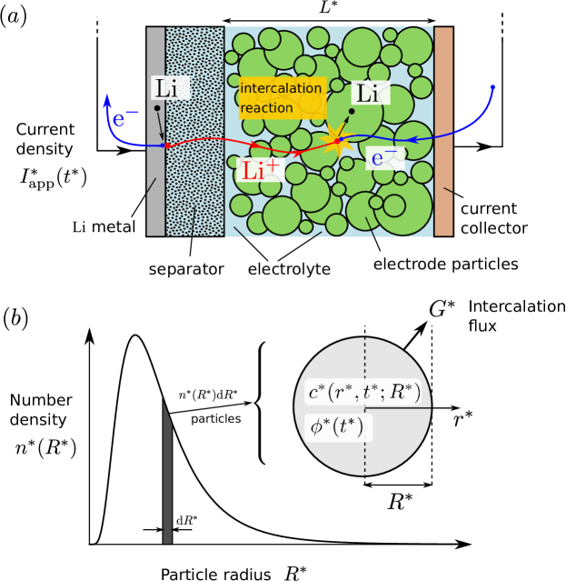
Figure 1: ($a$) The half cell under consideration; ($b$) the dimensional many-particle model (MPM) for a typical unimodal (log-normal) number density $n^{*}(R^{*})$.

We will consider a half-cell geometry, consisting of a single porous electrode immersed in a liquid electrolyte and separated from a lithium-metal electrode by an insulating porous separator, as depicted in Fig. 1$(a)$. In the small-current limit, the transport of lithium ions in the electrolyte is fast so they remain at a constant uniform concentration $c_{e}^{*}$ there. Here we use stars to denote that a quantity is dimensional. Only the lithium transport in the active material of the electrode, and the electrochemical reaction on the electrode–electrolyte interfaces, need to be modelled. First we describe the particle geometry and distribution, then state the electrochemical model.

2.1.1 Particle-Size Distribution (PSD)

The active particles that make up the porous electrode are assumed to be spherical but of a range of different sizes. In general, we assume there is a continuous distribution of particles of radii in the range $0<R^{*}<\infty$, with the number of particles (per unit electrode volume) with radii between $R^{*}$ and $R^{*}+\mathrm{d}R^{*}$ given by $n^{*}(R^{*})\mathrm{d}R^{*}$ [34]. The physical location of the particles in the electrodes is irrelevant because ion transport through the electrolyte is assumed instantaneous, and thus all particles of a given radius $R^{*}$ behave identically—see Fig. 1$(b)$. The particles could be, for example, distributed uniformly throughout the electrode or graded spatially by size, and the model presented here is applicable in both cases.

The surface area $A^{*}(R^{*})$ and volume $V^{*}(R^{*})$ of a particle of radius $R^{*}$ are, for spheres, given by

(1) $$A^{*}(R^{*}) =4\pi R^{*2}, V^{*}(R^{*}) =\frac{4}{3}\pi R^{*3},$$

from which an area density $a^{*}(R^{*})$ and volume density $v^{*}(R^{*})$ can be defined,

(2) $$a^{*}(R^{*}) =A^{*}(R^{*})n^{*}(R^{*}), v^{*}(R^{*}) =V^{*}(R^{*})n^{*}(R^{*}),$$

corresponding to the area and volume of all particles of radius $R^{*}$, respectively. The total particle number, surface area, and volume (each per unit volume of electrode) are given by

(3) $$n_{\mathrm{total}}^{*} =\int_{0}^{\infty}n^{*}(R^{*})\mathrm{d}R^{*}, a_{\mathrm{total}}^{*} =\int_{0}^{\infty}a^{*}(R^{*})\mathrm{d}R^{*}, v_{\mathrm{total}} =\int_{0}^{\infty}v^{*}(R^{*})\mathrm{d}R^{*}.$$

The quantity $a_{\mathrm{total}}^{*}$ is known as the specific surface area or Brunauer–Emmett–Teller (BET) surface area, while $v_{\text{total}}$ is dimensionless and corresponds to the volume fraction of active material, often denoted by $\epsilon_{s}$. We can normalise the densities $n^{*}$, $a^{*}$, and $v^{*}$ by their totals to give fraction densities

(4) $$f_{n}^{*}(R^{*})=\frac{n^{*}(R^{*})}{n_{\mathrm{total}}^{*}},\qquad f_{a}^{*}(R^{*})=\frac{a^{*}(R^{*})}{a_{\mathrm{total}}^{*}},\qquad f_{v}^{*}(R^{*})=\frac{v^{*}(R^{*})}{v_{\mathrm{total}}},$$

satisfying $\int_{0}^{\infty}f_{i}^{*}(R^{*})\mathrm{d}R^{*}=1$ for each of $i=n,a,v$. The quantity $f_{n}^{*}(R^{*})$ can be interpreted as the radius distribution, i.e., the probability density function of a particle having radius $R^{*}$ if randomly sampled from the population. However, $f_{a}^{*}(R^{*})$ and $f_{v}^{*}(R^{*})$ are not the area and volume distributions in this sense, and should instead be thought of as new radius distributions created by weighting $f_{n}^{*}(R^{*})$ by the area and volume, respectively, and then renormalising. Hence we shall refer to them as the area- and volume-weighted radius distributions; they are commonly used in place of $f_{n}^{*}(R^{*})$, depending on the experimental technique used to measure the PSD.

As the PSD is completely described by the number density $n^{*}(R^{*})$, we may specify the total number of particles, $n_{\mathrm{total}}^{*}$, and how they are distributed by radius, $f_{n}^{*}(R^{*})$, with the remaining quantities in (2)-(4) following from their definitions. One could, however, specify any one of (3) instead of $n_{\mathrm{total}}^{*}$, and we will choose $v_{\mathrm{total}}$, which is easiest to determine experimentally. It also influences the maximum theoretical capacity of the electrode, which we will keep fixed as we vary the shape and spread of the distribution. Substituting $a^{*}(R^{*})=n_{\mathrm{total}}^{*}4\pi R^{*2}f_{n}^{*}(R^{*})$ and $v^{*}(R^{*})=n_{\mathrm{total}}^{*}\frac{4}{3}\pi R^{*3}f_{n}^{*}(R^{*})$ into (3) and solving for $n_{\mathrm{total}}^{*}$ and $a_{\mathrm{total}}^{*}$ gives

(5) $$n_{\mathrm{total}}^{*}=\frac{v_{\mathrm{total}}}{\frac{4}{3}\pi\int_{0}^{\infty}R^{*3}f_{n}^{*}(R^{*})\mathrm{d}R^{*}},\qquad a_{\mathrm{total}}^{*}=\frac{3v_{\mathrm{total}}\int_{0}^{\infty}R^{*2}f_{n}^{*}(R^{*})\mathrm{d}R^{*}}{\int_{0}^{\infty}R^{*3}f_{n}^{*}(R^{*})\mathrm{d}R^{*}}.$$

It will be useful to introduce the raw moments

$$m_{i,j}^{*}=\int_{0}^{\infty}R^{*j}f_{i}^{*}(R^{*})\mathrm{d}R^{*},\qquad i=n,a,v,\quad j=1,2,\ldots$$

as well as the means (first raw moment) and variances

(6) $$\bar{R}_{i}^{*}=\mathbb{E}_{i}[R^{*}]=m_{i,1}^{*},\qquad\sigma_{i}^{*2}=\mathbb{E}_{i}[(R^{*}-\bar{R}_{i}^{*})^{2}]=m_{i,2}^{*}-m_{i,1}^{*2},\qquad i=n,a,v.$$

The mean $\bar{R}_{n}^{*}$ corresponds to the average particle radius. For further discussion about the means $\bar{R}_{i}^{*}$ and their physical meaning see §3.1.

2.1.2 Electrochemical model

The transport of lithium within a particle of radius $R^{*}$ is assumed to be spherically symmetric, and modelled by Fickian diffusion,

(7) $$\frac{\partial c^{*}}{\partial t^{*}} =D^{*}\frac{1}{r^{*2}}\frac{\partial}{\partial r^{*}}\left(r^{*2}\frac{\partial c^{*}}{\partial r^{*}}\right),\qquad\text{for }0<r^{*}<R^{*},$$

(8) $$c^{*} \equiv c_{\text{init}}^{*},\qquad\text{at }t^{*}=0,$$

where $c^{*}(r^{*},t^{*};R^{*})$ is the concentration of lithium in the solid electrode material, with initial uniform concentration $c_{\text{init}}^{*}$, and $D^{*}$ is the solid-state diffusion coefficient. There is a surface flux, i.e. lithium (de)intercalation into (out of) the particles,

(9) $$-D^{*}\frac{\partial c^{*}}{\partial r^{*}}=G^{*},\qquad\text{at }r^{*}=R^{*},$$

modelled by standard Butler–Volmer kinetics,

(10) $$G^{*}=\frac{k^{*}}{F^{*}}(c^{*})^{1/2}(c_{\text{max}}^{*}-c^{*})^{1/2}(c_{e}^{*})^{1/2}\sinh\left(\frac{F^{*}}{2R_{g}^{*}T^{*}}\eta^{*}\right),\qquad\text{at }r^{*}=R^{*}.$$

Here $F^{*}$ is Faraday’s constant, $R_{g}^{*}$ is the universal gas constant, $T^{*}$ is the temperature (assumed constant), $k^{*}$ is a reaction rate coefficient, $c_{\text{max}}^{*}$ is the maximum lithium concentration in the electrode material, $c_{e}^{*}$ is the concentration of lithium ions in the electrolyte (assumed constant), and the transfer coefficients for the anodic and cathodic reactions are taken to be one half. The function $\eta^{*}=\Delta\phi^{*}(t^{*})-U^{*}(c_{s}^{*},c_{e}^{*})$ is the surface overpotential, where $\Delta\phi^{*}(t^{*})$ is the potential difference between the electrode and the electrolyte (a function of time only since the electrical conductivities are assumed large), and $U^{*}(c_{s}^{*},c_{e}^{*})$ is the open circuit potential (OCP), an empirical function depending on $c_{e}^{*}$ and the local surface concentration $c_{s}^{*}(t;R)=c^{*}|_{r^{*}=R^{*}}$, typically found by fitting to experimental measurements relative to a Li/Li⁺ metal electrode—a half cell as modelled here. (As $c_{e}^{*}$ is assumed constant, the dependence of $U^{*}$ on $c_{e}^{*}$ will be subsequently suppressed.)

Finally, conservation of charge implies that the total lithium flux out of the electrode is proportional to the applied circuit current density, $I_{\text{app}}^{*}$. Since the surface area per unit electrode volume for the particles of radius $R^{*}$ is $a^{*}(R^{*})$, given by (2), charge conservation gives

(11) $$L^{*}\int_{0}^{\infty}a^{*}(R^{*})G^{*}(c_{s}^{*},\Delta\phi^{*})\,\mathrm{d}R^{*}=-\frac{I_{\text{app}}^{*}}{F^{*}},$$

where $I_{\text{app}}^{*}\gtrless 0$ corresponds to a discharge/charge current density for a cathode half cell (the opposite for an anode half cell), respectively, and $L^{*}$ is the through-cell thickness of the electrode (excluding separator and current collector; see Fig. 1$(a)$). If the current density $I_{\text{app}}^{*}$ is prescribed, then the unknown variables are $c^{*}(r^{*},t^{*};R^{*})$ for each particle size $R^{*}$, and the potential difference $\Delta\phi^{*}(t^{*})$, which is common to all particle sizes. If we choose the potential in the Li metal as our reference, then uniformity of the electrolyte potential gives $\phi_{e}^{*}\equiv 0$ and the half-cell potential is then simply $V_{\text{half-cell}}^{*}(t^{*})=\Delta\phi^{*}(t^{*})=\phi^{*}(t^{*})$.

The system (7)-(10) consists of a diffusion equation for each $0<R^{*}<\infty$, all coupled via the integral condition (11).

2.2 Scaling and nondimensional equations

We first identify the key timescales present in the problem. As our temporal scaling we use the characteristic discharge timescale for the cell, defined as

(12) $$\tau_{\text{d}}^{*}=\frac{F^{*}c_{\text{max}}^{*}L^{*}v_{\mathrm{total}}}{I_{\text{typ}}^{*}}.$$

This corresponds to the time taken for a current density $I_{\mathrm{typ}}^{*}$ to completely discharge the electrode from its theoretical maximum capacity. There is a diffusion and a reaction timescale,

(13) $$\tau_{\text{diff}}^{*}=\frac{(R_{\text{typ}}^{*})^{2}}{D^{*}},\qquad\tau_{\text{reac}}^{*}=\frac{F^{*}}{k^{*}a_{\text{typ}}^{*}(c_{e}^{*})^{1/2}},$$

respectively, where $R_{\text{typ}}^{*}$ and $a_{\text{typ}}^{*}$ are typical scales for the particle radii and surface area per unit electrode volume. We choose $a_{\mathrm{typ}}^{*}$ to be the surface area if all particles were of the typical radius, i.e., $a_{\text{typ}}^{*}=3v_{\mathrm{total}}/R_{\text{typ}}^{*}$. We will make different choices for $R_{\text{typ}}^{*}$ depending on whether the particle size distribution is unimodal or bimodal. For a unimodal particle size distribution, it is natural to take $R_{\text{typ}}^{*}=\overline{R}_{n}^{*}$, however, for a bimodal distribution it is more convenient to use a typical radius based on the average of just one of the modes or components—see §4.

Particle radii and radial coordinates are scaled with $R_{\text{typ}}^{*}$, concentrations with the maximum concentration $c_{\text{max}}^{*}$, time with the discharge timescale, potentials with $\Phi^{*}=1$ V, and the current density with $I_{\mathrm{typ}}^{*}$ (this allows the consideration of nonconstant applied current densities). The Butler–Volmer reaction rate is scaled based on the typical lithium flux required to sustain the current density $I_{\mathrm{typ}}^{*}$. By scaling the total surface area $a_{\mathrm{total}}^{*}$ with $a_{\text{typ}}^{*}$, natural scalings for all PSD quantities follow from their definitions (1)-(6) and appropriate powers of $R_{\mathrm{typ}}^{*}$. The resulting scalings are

$$r^{*} =R_{\text{typ}}^{*}r, (c^{*},c_{s}^{*},c_{\text{init}}^{*}) =c_{\text{max}}^{*}(c,c_{s},c_{\text{init}}), t^{*} =\tau_{\text{d}}^{*}t,$$

$$I_{\text{app}}^{*} =I_{\text{typ}}^{*}I, (\eta^{*},\Delta\phi^{*},U^{*}) =\Phi^{*}(\eta,\Delta\phi,U), G^{*} =\frac{I_{\text{typ}}^{*}}{F^{*}L^{*}a_{\mathrm{typ}}^{*}}G,$$

$$R^{*} =R_{\text{typ}}^{*}R, n_{\text{total}}^{*} =\frac{a_{\text{typ}}^{*}}{R_{\text{typ}}^{*2}}n_{\text{total}}, a_{\text{total}}^{*} =a_{\text{typ}}^{*}a_{\text{total}}, n^{*} =\frac{a_{\text{typ}}^{*}}{R_{\text{typ}}^{*3}}n,$$

$$a^{*} =\frac{a_{\text{typ}}^{*}}{R_{\text{typ}}^{*}}a, v^{*} =a_{\text{typ}}^{*}v, f_{i}^{*} =\frac{1}{R_{\text{typ}}^{*}}f_{i}, m_{i,j}^{*} =R_{\text{typ}}^{*j}m_{i,j},$$

which transform (7)-(11) into the nondimensional problem

(14) $$\frac{\partial c}{\partial t} =\gamma\frac{1}{r^{2}}\frac{\partial}{\partial r}\left(r^{2}\frac{\partial c}{\partial r}\right),\qquad\text{for }0<r<R,$$

(15) $$c =c_{\text{init}},\qquad\text{at }t=0,$$

with regularity at $r=0$ and boundary condition

(16) $$-\gamma\frac{\partial c}{\partial r} =\frac{1}{3}G(c,\Delta\phi)\qquad\text{at }r=R,$$

which are coupled via the $\Delta\phi$-dependence of their intercalation rates

(17) $$G(c_{s},\Delta\phi) =g(c_{s})\sinh\left\{\frac{\lambda}{2}\left[\Delta\phi-U(c_{s})\right]\right\},\qquad\displaystyle g(c_{s})=kc_{s}^{1/2}\left(1-c_{s}\right)^{1/2},$$

which must satisfy the total flux constraint

(18) $$\int_{0}^{\infty}a(R)G(c_{s},\Delta\phi(t))\mathrm{d}R=-I(t).$$

We remark that the factor of $1/3$ arises in boundary condition (16) (and in subsequent equations) because we consider spherical particles. For different particle shapes this numerical factor would be different.

All PSD relations (1)-(6) remain the same but with the stars now removed and the total active volume fraction, $v_{\mathrm{total}}$, replaced by $1/3$. In particular,

$$\int_{0}^{\infty}v(R)\mathrm{d}R=\frac{1}{3},\qquad f_{v}(R)=3v(R),$$

$$n_{\mathrm{total}}=\frac{1}{4\pi\int_{0}^{\infty}R^{3}f_{n}(R)\mathrm{d}R}=\frac{1}{4\pi m_{n,3}},\qquad a_{\mathrm{total}}=\frac{\int_{0}^{\infty}R^{2}f_{n}(R)\mathrm{d}R}{\int_{0}^{\infty}R^{3}f_{n}(R)\mathrm{d}R}=\frac{m_{n,2}}{m_{n,3}}=\frac{1}{\bar{R}_{a}}.$$

The nondimensional parameter groups introduced are

(19) $$\gamma =\frac{\tau_{\text{d}}^{*}}{\tau_{\text{diff}}^{*}}, k =\frac{\tau_{\text{d}}^{*}}{\tau_{\text{reac}}^{*}}, \lambda =\frac{F^{*}\Phi^{*}}{R_{g}^{*}T^{*}}.$$

The parameter $\lambda\approx 38.92$ is the ratio of the typical half cell voltage to the thermal voltage and is constant for the isothermal problem we consider. The parameters $\gamma$ and $k$ are ratios of the discharge timescale to the diffusion and reaction timescales, and they act as nondimensional diffusion and reaction coefficients in (14)-(18). Since both $\gamma$ and $k$ depend on the discharge time and thus the applied current, it can be useful to express them explicitly in terms of the so-called C-rate. If $\mathrm{C}^{*}$ is the current density that discharges the half-cell in 1 hour, then the C-rate is defined as $\mathcal{C}=I_{\mathrm{typ}}^{*}/\mathrm{C}^{*}$. Substituting $I_{\text{typ}}^{*}=\mathcal{C}\text{C}^{*}$ into (12), we can write $\gamma=\hat{\gamma}/\mathcal{C}$ and $k=\hat{k}/\mathcal{C}$ where $\hat{\gamma}$ and $\hat{k}$ depend only on the material parameters and geometry.

2.3 Fast diffusion in the electrode particles

The model may be simplified further if diffusion within the electrode particles is also fast in comparison to the discharge timescale, i.e. $\gamma=\tau_{\mathrm{d}}^{*}/\tau_{\mathrm{diff}}^{*}\gg 1$. In this case the MPM (14)-(18) reduces to a system of ODEs. It is straightforward to show in the limit $\gamma\to\infty$ that $c$ becomes independent of $r$. Then (14)-(18) becomes the system of mass balances

(20) $$\frac{\mathrm{d}c}{\mathrm{d}t} =\frac{A(R)}{3V(R)}G(c,\Delta\phi),\qquad 0<R<\infty,\ 0<t<\infty,$$

(21) $$c =c_{\mathrm{init}},\qquad\text{at }t=0,$$

(22) $$-I(t) =\int_{0}^{\infty}a(R)G(c,\Delta\phi)\mathrm{d}R,$$

where $A(R)$ and $V(R)$ are the surface area and volume of a particle of radius $R$. For spherical particles considered here, $A/(\text{3}V)=1/R$. If all the particles are the same shape but can be parametrised by a single length parameter $R$, then the system (20)-(22) in fact holds for particles of any shape, and $A/(3V)=\xi/R$ with the numerical constant $\xi$ depending on the shape.

2.4 Parameter values

For most of the paper we consider a graphite anode (meso-carbon microbeads or LiC₆) in an electrolyte consisting of LiPF₆ in the solvent EC:DMC of ratio 1:1 by volume. The parameters (taken from [25]) and resulting nondimensional parameters used are given in Tables 2 and 3 in appendix A, respectively. The functional expression for the open circuit potential $U^{*}(c_{s}^{*},c_{e}^{*})$ is taken from the Dualfoil code of Newman [30]. Later, in §4.3, we will also compare with experimental results on a lithium iron phosphate (LiFePO₄) cathode in the same electrolyte.

The shape of the PSD is specified by the radius distribution $f_{n}(R)$. We model a unimodal distribution as a log-normal (typical for electrode materials [26, 39]):

(23) $$f_{n}(R) =\frac{1}{R\sqrt{2\pi\sigma_{LN}^{2}}}\exp\left[-\frac{(\log R-\mu_{LN})^{2}}{2\sigma_{LN}^{2}}\right],\qquad\mu_{LN}\in(-\infty,\infty),\,\sigma_{LN}>0,$$

for which

(24) $$\bar{R}_{n} =\exp(\mu_{LN}+\sigma_{LN}^{2}/2),$$

(25) $$\sigma_{n}^{2} =\exp(\sigma_{LN}^{2}-1)\exp(2\mu_{LN}+\sigma_{LN}^{2}),$$

(26) $$m_{n,j} =\exp(j\mu_{LN}+j^{2}\sigma_{LN}^{2}/2),\qquad j=1,2,...$$

This can be described by only two parameters, the mean $\bar{R}_{n}$ and standard deviation $\sigma_{n}$. If $\bar{R}_{n}$ is fixed to be unity by the nondimensionalisation (i.e., $R_{\mathrm{typ}}^{*}=\bar{R}_{n}^{*}$), then in [6] fitting a log-normal to the PSDs of different graphite anode materials gave standard deviations in the range $0.15\leq\sigma_{n}\leq 1$. If we consider only meso-carbon microbeads (MCMB) [6], then this range is narrowed to $0.15\leq\sigma_{n}\leq 0.3$. Thus we will consider PSDs in the range of $\sigma_{n}\leq 0.3$ for graphite.

Results for Weibull distributions, also commonly used for PSDs [38], were found to be very similar for the values of $\sigma_{n}$ considered in this paper. The bimodal distributions in §4 are constructed from two log-normal distributions, one for each mode.

3 Unimodal Particle-Size Distributions

In this section we consider PSDs that are unimodal, such as that in Fig. 1$(b)$, and derive and assess several candidate asymptotic solutions in the limit where the distribution is narrow. We begin by discussing approximations of the PSD using particles of a single size, and then seek asymptotic corrections to a selection of these.

3.1 Single particle models (SPMs)

It is commonplace in porous electrode theory to assume that all the active electrode particles are of the same size. This reduces the computational complexity considerably, but the question of which particle radius best represents the full PSD is rarely considered. The model (14)-(18) reduces to the single particle model (SPM) when $f_{n}(R)=\delta(R-R^{\mathrm{SPM}})$, where $\delta$ is the Dirac $\delta$-function. Then, with $c(r,t,R^{\mathrm{SPM}})=c^{\textrm{SPM}}(r,t)$,

(27) $$\frac{\partial c^{\textrm{SPM}}}{\partial t} =\gamma\frac{1}{r^{2}}\frac{\partial}{\partial r}\left(r^{2}\frac{\partial c^{\textrm{SPM}}}{\partial r}\right),\qquad\text{for }0<r<R^{\mathrm{SPM}},$$

(28) $$-\gamma\frac{\partial c^{\textrm{SPM}}}{\partial r} =\frac{1}{3}G^{\mathrm{SPM}}(c^{\textrm{SPM}},\Delta\phi^{\mathrm{SPM}})\qquad\text{at }r=R^{\mathrm{SPM}},$$

with regularity at $r=0$, $c^{\textrm{SPM}}=c^{\textrm{SPM}}_{\text{init}}$ at $t=0$, and the surface flux $G^{\mathrm{SPM}}$ given by

(29) $$-I(t)=a_{\mathrm{total}}^{\mathrm{SPM}}G^{\mathrm{SPM}},$$

while

(30) $$n_{\mathrm{total}}^{\mathrm{SPM}}=\frac{1}{4\pi(R^{\mathrm{SPM}})^{3}},\qquad a_{\mathrm{total}}^{\mathrm{SPM}}=\frac{1}{R^{\mathrm{SPM}}}.$$

Recall that we choose the number of particles (and hence surface area) so as to fix the total volume, hence (30) depend on the particle radius.

As the surface flux is known exactly in terms of the current density, $I(t)$, the solution is very straightforward if one prescribes $I(t)$, since one can solve (27)-(28) for $c^{\textrm{SPM}}$ first then rearrange (29) for the potential:

(31) $$\Delta\phi^{\mathrm{SPM}}=U(c_{s}^{\mathrm{SPM}})-\frac{2}{\lambda}\sinh^{-1}\left[\frac{R^{\mathrm{SPM}}I(t)}{g(c_{s}^{\mathrm{SPM}})}\right].$$

This is considerably simpler than the full MPM (14)-(18), which has a continuum of PDEs coupled via an integral equation, even for prescribed $I(t)$.

The possible choices of $R^{\mathrm{SPM}}$ to represent the PSD are numerous and should be motivated by the application. From the theory of PSD characterisation, particularly that of droplets where many physical processes may be important [3], most of the important average radii are encapsulated by the following two parameter family, in terms of the moments of $f_{n}(R)$:

(32) $$R[p,q] =\left(\frac{\int_{0}^{\infty}R^{p}f_{n}(R)\mathrm{d}R}{\int_{0}^{\infty}R^{q}f_{n}(R)\mathrm{d}R}\right)^{1/(p-q)}=\left(\frac{m_{n,p}}{m_{n,q}}\right)^{1/(p-q)},\quad p\not=q=0,1,2,\ldots.$$

In this framework, $R[1,0]$ is simply the mean radius, i.e., the mean $\bar{R}_{n}$ of the distribution $f_{n}(R)$. The mean $R[2,0]$ corresponds to the radius of a sphere with area equal to the average area of the PSD. Similarly, $R[3,0]$ is the radius of a sphere with volume equal to the average volume of the PSD. For means of the form $R[p,0]$, knowledge of the number of particles (in a representative sample) is necessary. Thus they are all determined with similar measurement techniques, e.g., microscopy and image analysis [2], where individual particles are able to be counted.

A commonly used radius is $R[3,2]$, known as the Sauter mean radius [3] or surface-area moment mean,

(33) $$R[3,2] =\frac{\int_{0}^{\infty}R^{3}f_{n}(R)\mathrm{d}R}{\int_{0}^{\infty}R^{2}f_{n}(R)\mathrm{d}R}=\frac{3\mathbb{E}_{n}[V]}{\mathbb{E}_{n}[A]}=\frac{3\cdot\frac{1}{3}}{a_{\mathrm{total}}}=\frac{1}{a_{\mathrm{total}}},$$

which corresponds here to $\bar{R}_{a}$, the mean of the area-weighted radius distribution $f_{a}(R)$. It is widely used for applications where the active surface area is relevant, such as catalysis and combustion of liquid sprays [43]. Its definition is proportional to the ratio of the average volume $\mathbb{E}_{n}[V]$ to the average surface area $\mathbb{E}_{n}[A]$—it corresponds to the radius of a particle that has the same surface-area-to-volume ratio as the PSD [22]. As we have already fixed the total electrode volume, this means it is the unique radius that gives the same total surface area $a_{\mathrm{total}}$ as the PSD.

Another important radius, $R[4,3]$, is known as the de Brouckere mean radius [3] or volume moment mean,

(34) $$R[4,3] =\frac{\int_{0}^{\infty}R^{4}f_{n}(R)\mathrm{d}R}{\int_{0}^{\infty}R^{3}f_{n}(R)\mathrm{d}R},$$

and corresponds here to $\bar{R}_{v}$, the mean of the volume-weighted radius distribution $f_{v}(R)$. It is used when the bulk volume is considered more relevant, used also for combustion [43]. Typically $R[4,3]>R[3,2]$, i.e., $\bar{R}_{v}>\bar{R}_{a}$, and so an SPM of radius $\bar{R}_{v}$ has a lower surface area than the PSD (see (30)). However, $f_{v}(R)$ (and hence $\bar{R}_{v}$) is measured directly by laser diffraction analysis—one of the most common and accurate modern PSD analysis techniques [23]—and hence has significant practical relevance. Indeed, it is also generated by any measurement technique that is based on mass, such as sieving and sedimentation [2].

The relative sizes of these different means are shown in Table 1, given a mean radius $\bar{R}_{n}=1$ and standard deviation $\sigma_{n}=0.3$. Other mean radii, e.g. $R[2,1]$, $R[3,1]$, and those based on percentiles have no particular significance in this context and we do not consider them here.

Mean radius	$R[1,0]$	$R[2,0]$	$R[3,0]$	$R[3,2]$	$R[4,3]$	$R[5,3]$
Value	1	1.044	1.091	1.188	1.295	1.352

Table 1: Sizes of mean radii discussed in §3.1 for a log-normal distribution $f_{n}(R)$ with mean $\bar{R}_{n}=R[1,0]=1$ and standard deviation $\sigma_{n}=0.3$.

3.1.1 Equivalent capacity radius

In the present context we can identify another mean radius that arises naturally from charge capacity considerations. As shown by Röder et al [38], the spread of a PSD can have a significant effect on the discharge capacity of the half-cell. We will show that

(35) $$\bar{R}_{c}=R[5,3] =\left(\frac{\int_{0}^{\infty}R^{5}f_{n}(R)\mathrm{d}R}{\int_{0}^{\infty}R^{3}f_{n}(R)\mathrm{d}R}\right)^{1/2},$$

is the radius that, when used in an SPM, will exhibit a similar capacity to the full PSD if $\gamma$ is large, which is usually the case except at high C-rates (see Table 3). We make the argument for a discharging anode, but a similar argument holds whether charging or discharging an anode or cathode.

For a constant current discharge of an anode, we have $I=-1$, and the lithium leaves the electrode particles causing $c(r,t;R)$ to decrease and the potential $\Delta\phi(t)$ to increase. As the surface concentration $c_{s}$ of any particle approaches zero, $\Delta\phi\to\infty$, and since $\Delta\phi$ is the same for all particles, this can only happen if $c_{s}\to 0$ for all particles simultaneously. This occurs in finite time, say at $t=t_{\mathrm{f}}$, and any lithium still remaining inside the particles is not accessed. The proportion remaining is larger for slower lithium diffusion within the particles, larger particles, or higher C-rates. To estimate the amount of lithium remaining at final time, we use the approximate solution for $\gamma\gg 1$. Substituting a regular expansion of $c$ in powers of $\gamma^{-1}$ into (14)-(16) results in

(36) $$c(r,t;R)=c_{0}(t;R)+\frac{1}{\gamma}\frac{\mathrm{d}c_{0}}{\mathrm{d}t}\left(\frac{1}{6}r^{2}+B(t)\right)+\cdots,\qquad\gamma\gg 1,$$

where $c_{0}(t;R)$ is the solution of the fast diffusion problem (20)-(22), and $B(t)$ is a nontrivial function of $t$ which will not be needed. Setting $c=0$ on the surface $r=R$ at time $t=t_{\mathrm{f}}$, and subtracting from (36) at $t=t_{\mathrm{f}}$ gives

(37) $$c(r,t_{\mathrm{f}};R)=\frac{1}{6\gamma}\left.\frac{\mathrm{d}c_{0}}{\mathrm{d}t}\right|_{t_{\mathrm{f}}}\left(r^{2}-R^{2}\right)+\cdots,\qquad\gamma\gg 1.$$

Integrating this over all the particles and dividing by the maximum capacity, we find the fraction $\mathcal{F}_{\mathrm{cap}}$ remaining at $t=t_{\mathrm{f}}$ to be

(38) $$\mathcal{F}_{\mathrm{cap}}=\frac{\int_{0}^{\infty}n(R)(\int_{0}^{R}4\pi r^{2}c\,\mathrm{d}r)\,\mathrm{d}R}{\int_{0}^{\infty}V(R)n(R)\,\mathrm{d}R}=\frac{1}{15\gamma}\frac{\int_{0}^{\infty}(\mathrm{d}c_{0}/\mathrm{d}t)R^{5}f_{n}(R)\,\mathrm{d}R}{\int_{0}^{\infty}R^{3}f_{n}(R)\mathrm{d}R}+\cdots,\qquad\gamma\gg 1.$$

Now, $c_{0}$ itself hits zero slightly later at $t_{\mathrm{f},0}=t_{\mathrm{f}}+O(\gamma^{-1})>t_{\mathrm{f}}$, where we have

(39) $$c_{0}\sim(t-t_{\mathrm{f},0}),\qquad G_{0}\sim R,\qquad\Delta\phi_{0}\sim-\frac{2}{\lambda}\log(t-t_{\mathrm{f},0}),\qquad\text{as }t\to t_{\mathrm{f},0}^{+}.$$

Thus, $\left.(\mathrm{d}c_{0}/\mathrm{d}t)\right|_{t_{\mathrm{f}}}=1+O(\gamma^{-1})$, which substituted into (38) gives

(40) $$\mathcal{F}_{\mathrm{cap}}=\frac{(R[5,3])^{2}}{15\gamma}+\cdots,\qquad\gamma\gg 1.$$

Repeating the analysis for the SPM is simpler, resulting in the fraction

(41) $$\mathcal{F}_{\mathrm{cap}}^{\mathrm{SPM}}=\frac{(R^{\mathrm{SPM}})^{2}}{15\gamma}+\cdots,\qquad\gamma\gg 1.$$

Thus we identify the mean radius $\bar{R}_{c}=R[5,3]$ as that which would give the correct capacity remaining when used in an SPM.

For practical purposes, $\bar{R}_{c}$ may be calculated easily from the volume-weighted distribution via

(42) $$\bar{R}_{c}=(m_{v,2})^{1/2}=(\bar{R}_{v}^{2}+\sigma_{v}^{2})^{1/2}.$$

and can be interpreted as the radius that gives the average surface area when calculated using the volume-weighted distribution $f_{v}$.

3.2 Corrections to single particle models for narrow distributions

The SPM, with a given choice of effective particle radius, is the leading-order approximation as $\sigma_{n}\rightarrow 0$, that is, when the unimodal PSD is narrow and most particles are clustered close to that single radius. In this section we seek an asymptotic correction to this SPM. We present the analysis for the area-weighted mean $\bar{R}_{a}$ as it is the simplest, with the corresponding results for $\bar{R}_{n}$ and $\bar{R}_{v}$ given in the Supplementary Material. We find it more convenient to use $\sigma_{a}$ as the small parameter here, noting that $\sigma_{a}=O(\sigma_{n})$ as $\sigma_{n}\rightarrow 0$.

In terms of the area-weighted distribution the integral constraint (18) is

(43) $$-I(t)=\frac{1}{\bar{R}_{a}}\int_{0}^{\infty}f_{a}(R)G(c_{s}(t;R),\Delta\phi(t))\mathrm{d}R.$$

In the limit $\sigma_{a}\to 0$, $f_{a}$ will become concentrated around $R=\bar{R}_{a}$ and therefore we Taylor expand the integrand (but not the distribution $f_{a}$ itself) about this value

$$G=G_{a}+(R-\bar{R}_{a})\left(\frac{\partial G}{\partial R}\right)_{a}+\frac{1}{2!}(R-\bar{R}_{a})^{2}\left(\frac{\partial^{2}G}{\partial R^{2}}\right)_{a}+O((R-\bar{R}_{a})^{3}),$$

where the subscript $a$ denotes evaluation at $R=\bar{R}_{a}$. Substituting into (43) and assuming $\sigma_{a}$ is sufficiently small so we can integrate term-by-term gives

(44) $$-I(t)= \frac{1}{\bar{R}_{a}}\left[G_{a}+\frac{1}{2}\left(\frac{\partial^{2}G}{\partial R^{2}}\right)_{a}\sigma_{a}^{2}+O(\sigma_{a}^{3}\tilde{\mu}_{3,a})\right].$$

Truncating the Taylor expansion produces an error due to the skewness, which is $O(\sigma_{a}^{3}\tilde{\mu}_{3,a})=O(\sigma_{a}^{4})$ for a log-normal (23), but we have not yet formally expanded in $\sigma_{a}$. We do so now, expanding all variables in powers of $\sigma_{a}^{2}$ as

(45) $$G=G^{(0)}+\sigma_{a}^{2}G^{(2)}+\cdots,$$

etc. At leading order $G_{a}^{(0)}=-\bar{R}_{a}I(t)$, which gives exactly the SPM (27)-(31) with radius $R=\bar{R}_{a}$ as expected. At $O(\sigma_{a}^{2})$ we find

(46) $$G_{a}^{(2)}=-\frac{1}{2}\left(\frac{\partial^{2}G^{(0)}}{\partial R^{2}}\right)_{a},$$

so that the correction $G_{a}^{(2)}$ to the boundary flux for $R=\bar{R}_{a}$ is given in terms of the second derivative of $G^{(0)}$ with respect to particle radius $R$ evaluated at $R=\bar{R}_{a}$. Since the SPM (27)-(31) has $R\equiv\bar{R}_{a}$, to evaluate this second derivative we need to solve (two) additional problems, which we describe next. We consider the cases of fast and non-fast solid diffusion separately.

3.2.1 Calculation of $(\partial^{2}G^{(0)}/\partial R^{2})_{a}$ for fast diffusion

When solid diffusion within the particles is fast, the governing equations reduce to (20)-(22), with $R$ appearing as a parameter in the ODEs. In this case, we may differentiate (20) directly with respect to $R$, noting that $G(c,\Delta\phi)$ depends on $R$ only through $c$, to give

(47) $$\left[\frac{\mathrm{d}}{\mathrm{d}t}+\frac{1}{R}\frac{\partial G}{\partial c}\right]\left(\frac{\partial c}{\partial R}\right) =\frac{1}{R^{2}}G,$$

(48) $$\left[\frac{\mathrm{d}}{\mathrm{d}t}+\frac{1}{R}\frac{\partial G}{\partial c}\right]\left(\frac{\partial^{2}c}{\partial R^{2}}\right) =-\frac{1}{R}\frac{\partial^{2}G}{\partial c^{2}}\left(\frac{\partial c}{\partial R}\right)^{2}+\frac{2}{R^{2}}\frac{\partial G}{\partial c}\frac{\partial c}{\partial R}-\frac{2}{R^{3}}G.$$

If we now substitute $R=\bar{R}_{a}$, and the leading order solutions for $c_{a}^{(0)}$ and $\Delta\phi^{(0)}$ into $G$ and its derivatives, equations (47) and (48) form two ODEs for the unknowns $(\partial c^{(0)}/\partial R)_{a}$ and $(\partial^{2}c^{(0)}/\partial R^{2})_{a}$, from which we can determine $(\partial^{2}G^{(0)}/\partial R^{2})_{a}$ using the chain rule, i.e.

(49) $$\frac{\partial^{2}G}{\partial R^{2}} =\frac{\partial^{2}G}{\partial c^{2}}\left(\frac{\partial c}{\partial R}\right)^{2}+\frac{\partial G}{\partial c}\frac{\partial^{2}c}{\partial R^{2}}.$$

Expressions for $\partial G/\partial c$ and $\partial^{2}G/\partial c^{2}$ are given in §C.

3.2.2 Calculation of $(\partial^{2}G^{(0)}/\partial R^{2})_{a}$ for non-fast diffusion

When diffusion within the particles is not instantaneous it is easiest to approximate $\partial^{2}G/\partial R^{2}$ by solving (27)-(28) for radii either side and close to the mean, $R=\bar{R}_{a}\pm\Delta R$, given the leading-order potential $\Delta\phi^{(0)}$. From the solutions $c_{a,\pm}^{(0)}$ for these neighbouring radii, we can then approximate the derivative using finite differences, e.g.

(50) $$\left(\frac{\partial^{2}G^{(0)}}{\partial R^{2}}\right)_{a} =\frac{G(c_{a,+,s}^{(0)},\Delta\phi^{(0)})-2G_{a}^{(0)}+G(c_{a,-,s}^{(0)},\Delta\phi^{(0)})}{\Delta R}+O(\Delta R^{2}).$$

This approach is applicable to any form of lithium transport within the particles since (50) applies only on the surface and has the advantage that the auxiliary problems are also single particle problems, but with a different particle radius. It is preferable to a direct boundary perturbation analysis for $R$ close to $\bar{R}_{a}$, which involves significant algebra (as one must proceed to second order) and computational difficulties in capturing the behaviour at the particle surface, where spatial gradients become successively larger at higher orders.

3.2.3 Corrected potential

Given $G_{a}^{(2)}$ from (46), the problem for the correction to the concentration $c_{a}^{(2)}$ at the radius $R=\bar{R}_{a}$ is similar to that at leading order, but with a vanishing initial condition,

(51) $$\frac{\partial c_{a}^{(2)}}{\partial t} =\frac{\gamma}{r^{2}}\frac{\partial}{\partial r}\left[r^{2}\frac{\partial c_{a}^{(2)}}{\partial r}\right], 0<r <\bar{R}_{a},0<t$$

(52) $$-\gamma\frac{\partial c_{a}^{(2)}}{\partial r} =\frac{1}{3}G_{a}^{(2)}, \text{at }r =\bar{R}_{a},$$

(53) $$c_{a}^{(2)} =0, \text{at }t =0,$$

with regularity ar $r=0$. The potential can then be updated analytically using (17) and substituting $c_{a,s}=c_{a,s}^{(0)}+\sigma_{a}^{2}c_{a,s}^{(2)}+O(\sigma_{a}^{4})$ and $G_{a}=G_{a}^{(0)}+\sigma_{a}^{2}G_{a}^{(2)}+O(\sigma_{a}^{4})$, giving

(54) $$\Delta\phi=U(c_{a,s}^{(0)}+\sigma_{a}^{2}c_{a,s}^{(2)})+\frac{2}{\lambda}\sinh^{-1}\left[\frac{G_{a}^{(0)}+\sigma_{a}^{2}G_{a}^{(2)}}{g(c_{a,s}^{(0)}+\sigma_{a}^{2}c_{a,s}^{(2)})}\right]+O(\sigma_{a}^{4}).$$

We could Taylor expand this for $\sigma_{a}\ll 1$ but, since it is already explicit, we keep it in unexpanded form to avoid magnified errors near electrode depletion or saturation, where $U$ is singular.

3.3 Results

To study heterogeneity due to the PSD, and also assess the validity of the single particle models and their asymptotic corrections, we consider a constant current discharge of a graphite anode half-cell, with parameters given in Tables 2 and 3. During discharge, lithium deintercalates from the electrode particles, which begin at a uniform lithium concentration of $c_{\mathrm{init}}=0.8$, and the half-cell potential $\Delta\phi^{*}$ increases until a cut-off value of 0.6 V. The mean radius $\bar{R}_{n}$ is fixed to be one, and the spread of the PSD is then controlled via the single parameter $\sigma_{n}$.

3.3.1 Numerical methods

The full MPM model (14)-(18), each SPM model (27)-(31) and their corrections in §3.2 were solved numerically using a finite-volume discretisation within each particle (with 30 volumes being sufficient) and an adaptive explicit ODE solver in MATLAB for time integration. The solver ode15s was used due to the presence of the algebraic equation resulting from the integral constraint (18), which we discretise assuming a finite number of particle sizes, $N$, equispaced between $R=0$ and $R=\bar{R}_{n}+10\sigma_{n}$ (excluding $R=0$). Then $N$ was increased until convergence, with $N=75$ sufficient for graphical accuracy. When diffusion is fast and the model reduces to ODEs, the computations are simpler, and $N=300$ was taken for the results presented here.

3.3.2 Fast diffusion

First we consider the case (20)-(22) where the diffusion in the particles is fast. A plot of the typical evolution of the concentrations $c(t;R)$ throughout the discharge is shown in Fig. 3, for a C-rate $\mathcal{C}=1$ and log-normal PSD with standard deviation $\sigma_{n}=0.3$ (shown in Fig. 2). The behaviour shown in Fig. 3$(a)$ can be understood with reference to the OCP for graphite, $U(c)$, which has several steps—quick transitions between plateaus (see Fig. 3$(b)$). Smaller particles deplete faster due to their larger surface-area-to-volume ratio, until their lithium concentration reaches a steeper section of the OCP. Their reaction resistance increases and deintercalation shifts to the larger particles. When the lithium concentration in all particles is again comparable, the smaller particles deplete more quickly again and the process repeats. Thus we see in 3$(a)$ an irregular and staggered depletion of smaller particles, with larger particles depleting more smoothly.

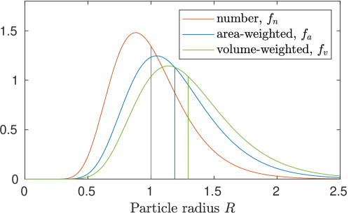
Figure 2: Log-normal particle size (number) distribution $f_{n}(R)$ with $\bar{R}_{n}=1$ and $\sigma_{n}=0.3$, and corresponding area-weighted- and volume-weighted-distributions $f_{a}$,$f_{v}$. Vertical lines indicate the location of their means, $\bar{R}_{n}=1$, $\bar{R}_{a}=1.188$, $\bar{R}_{v}=1.295$.

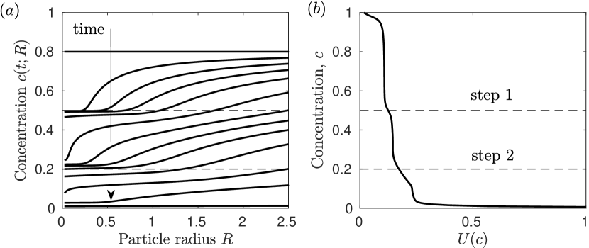
Figure 3: A 1C discharge of a graphite anode (fast diffusion $\gamma=\infty$), for PSD in Fig. 2: $(a)$ concentrations at selected times and $(b)$ OCP of graphite, $U(c)$. The concentrations corresponding approximately to the “steps” of $U(c)$ are indicated with dashed lines.

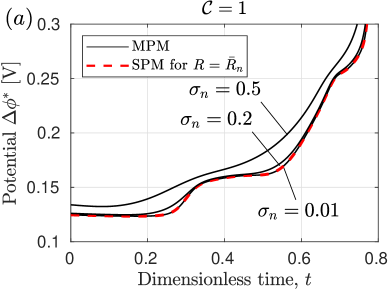
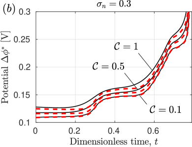
Figure 4: Cell potential throughout a discharge (fast diffusion $\gamma=\infty$), showing MPM and SPM (at $\bar{R}_{n}$) results for: $(a)$ various $\sigma_{n}$ with C-rate $\mathcal{C}=1$; $(b)$ various $\mathcal{C}$ with $\sigma_{n}=0.3$.

The consequences for the cell potential are shown in Fig. 4. As $\sigma_{n}$ is increased, the increasingly nonuniform discharge results in both an increase and a smoothing of the potential (Fig. 4$(a)$). This effect was not observed by Röder et al. [38], as they used an analytical (logarithmic) expression for $U(c)$ for graphite where the “steps” seen in the empirical $U(c)$ are absent. Furthermore, for a given $\sigma_{n}>0$, the smoothing near the steps is enhanced as the C-rate $\mathcal{C}$ increases, as seen in Fig. 4$(b)$. This smoothing effect cannot be captured by an SPM. Finally we note that the effect of PSD spread on the discharge capacity of the electrode is negligible (not shown), since when diffusion is fast all the intercalated lithium can be accessed.

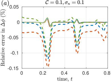
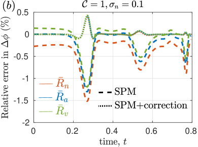
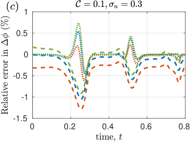
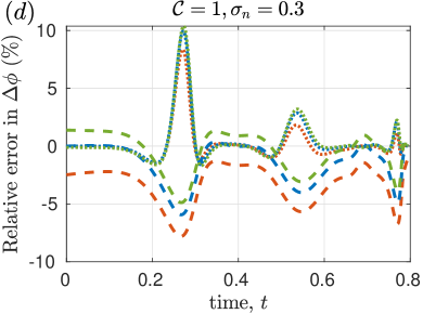
Figure 5: Signed error in cell potential relative to MPM throughout a discharge (fast diffusion $\gamma=\infty$), of SPM (dashed lines) and SPM corrected for narrow distributions (dotted lines). Results for the mean radius $\bar{R}_{n}$ (red), area-weighted mean radius $\bar{R}_{a}$ (blue), and volume-weighted mean radius $\bar{R}_{v}$ (green). Different panels are for $\sigma_{n}=0.1,0.3$ and C-rate $\mathcal{C}=0.1,1$, indicated.

To assess the extent to which the SPMs and their corrections for narrow distributions can approximate the aforementioned behaviour, we plot the error of each relative to the MPM throughout the discharge, shown in Fig. 5, for different $\sigma_{n}$ and $\mathcal{C}$. Each SPM (dashed lines) exhibits a significant negative error (thus underestimate) around $t=0.25$ and $0.55$, where the concentration in the particles passes the steps in $U(c)$, because the SPMs cannot capture the smoothing effect. Away from the steps, where $U(c)$ is relatively flat, the SPMs at $\bar{R}_{n}$ and $\bar{R}_{v}$ under- and overestimate the potential, with the SPM at $\bar{R}_{a}$ being the most accurate. As described in §3.1, this is because $\bar{R}_{a}$ is the unique radius that gives the same surface area as the PSD, and hence the same reaction resistance if the concentration in every particle is the same, which is true initially and after every step in $U(c)$.

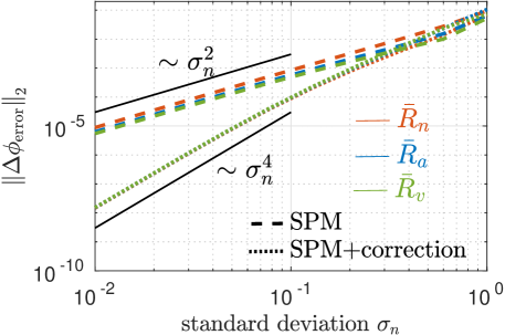
Figure 6: Global $L^{2}$-error, $||\Delta\phi_{\mathrm{error}}||_{2}=\left(\int\Delta\phi_{\mathrm{error}}^{2}\mathrm{d}t\right)^{1/2},$ in cell potential relative to MPM throughout a discharge (fast diffusion $\gamma=\infty$) of SPMs and SPMs corrected for narrow distributions, $\sigma_{n}\ll 1$. See legend and caption of Fig. 5. C-rate is $\mathcal{C}=1$.

The corrected SPMs for narrow distributions (dotted lines in Fig. 5) show a significant improvement in accuracy over the SPMs away from the steps of $U(c)$, for any choice of effective radius. However, as $\sigma_{n}$ or $\mathcal{C}$ is increased, the corrected SPMs begin to overcorrect for the smoothing of the steps and the approximation breaks down locally. This demonstrates the difficulty in capturing the smoothing effect using the dynamics only close to the mean radius. In particular, approximating the concentrations $c$ and surface fluxes $G$ with a Taylor expansion in $R$ about a mean quickly fails to predict the behaviour of particles across the spread of the PSD as $\sigma_{n}$ increases. Despite this local error, the global error, e.g. the L²-norm of the error over the entire discharge, shown in Fig. 6, behaves as expected. The L²-error is $O(\sigma_{n}^{2})$ for the SPMs and $O(\sigma_{n}^{4})$ for their corrections, with a global improvement over the SPMs for $\sigma_{n}\leq 0.3$, a physically relevant range.

3.3.3 Non-fast diffusion

We now consider the full MPM problem (14)-(18), accounting for diffusion in the particles. In this case, as well as the effects described in §3.3.2, there is an additional, more significant, effect on the usable capacity, as observed by Röder et al. [38] for a similar model. The usable capacity is calculated by Coulomb counting, i.e. integrating the applied current density in time until voltage cut-off. The amount discharged by any particular time is the depth of discharge, expressed here as a percentage of the theoretical maximum, $F^{*}c_{\mathrm{init}}^{*}L^{*}v_{\mathrm{total}}$. As discussed in §3.1.1, at the end of discharge, the surface concentration $c_{s}$ of each particle approaches zero, and the finite diffusivity results in lithium remaining in the particle cores, unaccessed. Fig. 7 shows a typical concentration distribution at voltage cut-off, with higher concentrations remaining in larger particles.

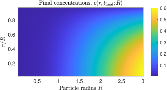
Figure 7: Nondimensional distribution of lithium throughout the particles at the end of discharge (at voltage cut-off), for a log-normal distribution (shown in Fig. 3) with mean $\bar{R}_{n}=1$ and standard deviation $\sigma_{n}=0.3$, and C-rate $\mathcal{C}=1$.

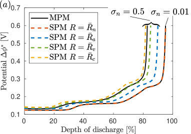
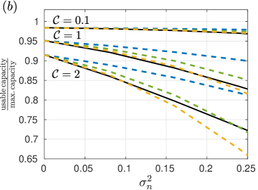
Figure 8: $(a)$ Cell potential of the MPM (solid) and several SPMs (dashed) throughout the discharge with diffusion in the particles, C-rate $\mathcal{C}=1$; $(b)$ Fraction of maximum theoretical capacity discharged by voltage cut-off. Mean radii as in caption 5, with addition of equivalent capacity radius $\bar{R}_{c}$, given by (35).

The potential, and the fraction of the theoretical capacity utilized, are shown in Fig. 8, for various $\sigma_{n}$. Increasing $\sigma_{n}$ results in a compression of the discharge curve horizontally and an earlier arrival at the cut-off voltage. Hence the greatest capacity is achieved as $\sigma_{n}\to 0$, i.e. when all the particles are of the mean radius $\bar{R}_{n}=1$. The capacity effects can be well reproduced by an SPM with judicious choice of radius. Results for SPMs at typical mean radii $\bar{R}_{n}$, $\bar{R}_{a}$ and $\bar{R}_{v}$, along with the newly-derived equivalent-capacity radius $\bar{R}_{c}$ (see §3.1.1) are compared to the full MPM in Fig. 8. The mean radius itself, $\bar{R}_{n}$, performs the worst, as it is independent of $\sigma_{n}$ and shows no decrease in capacity (for clarity it is not included in Fig. 8($b$)). The radii $\bar{R}_{a}$ and $\bar{R}_{v}$ perform better, and were discussed by Röder et al. [38], but the new radius $\bar{R}_{c}$ predicts capacity the best, and for a wide range of C-rates, despite its derivation being based on a low C-rate. For a given value of $\gamma$, however, the approximation breaks down as $\sigma_{n}$ increases and progressively larger particles are included. Nonetheless, use of $\bar{R}_{c}$ is excellent up to $\sigma_{n}\approx 0.5$ if $\mathcal{C}\leq 1$ or $\sigma_{n}\approx 0.4$ if $\mathcal{C}\leq 2$.

One drawback of using the mean radius $\bar{R}_{c}$ is that it underestimates the surface area compared to the actual PSD. This means, near the beginning of a discharge, before capacity considerations become important, $\bar{R}_{c}$ overestimates the reaction resistance and hence the cell voltage. Here, it is $\bar{R}_{a}$ that best predicts the voltage, just as for the case of fast diffusion—see §3.3.2.

Asymptotic corrections to the SPMs for narrow distributions serve to only correct for the shape (i.e. smoothness) of the discharge curve, exhibiting very similar behaviour (and drawbacks) to those for fast diffusion, and hence we do not present them here. They do not correct for errors in capacity due to incorrect choice of radius, highlighting the fact that the choice of effective radius is crucial when approximation an MPM with an SPM.

3.3.4 Local concentrations and current densities

The solution (31) for the potential $\Delta\phi^{\mathrm{SPM}}(t)$ for an SPM with particle radius $R=R^{\mathrm{SPM}}$ is an estimate for the potential $\Delta\phi(t)$ of the full MPM. This $\Delta\phi$ is the same for all particles, hence approximate solutions for the concentrations in particles of size $R\neq R^{\mathrm{SPM}}$, denoted $c^{(0)}(r,t;R)$, can be calculated by substituting $\Delta\phi\sim\Delta\phi^{\mathrm{SPM}}$ into (14)-(16) giving

(55) $$\frac{\partial c^{(0)}}{\partial t} =\frac{\gamma}{r^{2}}\frac{\partial}{\partial r}\left[r^{2}\frac{\partial c^{(0)}}{\partial r}\right], 0<r <R,\quad 0<t$$

(56) $$-\gamma\frac{\partial c^{(0)}}{\partial r} =\frac{1}{3}G(c^{(0)},\Delta\phi^{\mathrm{SPM}}), \text{at }r =R,$$

with $c^{(0)}$ regular at the origin and $c^{(0)}=c_{\mathrm{init}}$ at $t=0$. There are several advantages to approximating the problem in this way: (i) each particle size $R$ is decoupled from the others since the integral equation (18) has been eliminated; in particular they can be trivially parallelized; (ii) the dynamics of particles of any particular size can be investigated and solved for individually without needing to solve for all particles; (iii) it allows use of an SPM for battery control and fast online management, with after-the-fact computation of heterogeneous internal states, and thus nonuniform degradation rates, and at as few (or many) particle sizes as desired. It has been suggested that variations in rates of exfoliation and SEI layer growth (common mechanisms of electrode degradation) from particle to particle are due to local variations in surface current density [19]. In nondimensional terms, this corresponds to $G$, which can be approximated for any $R$ from the solution of (55)-(56).

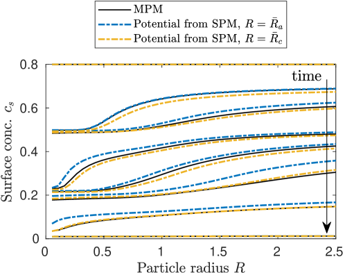
Figure 9: Surface concentrations at selected times throughout a discharge, comparing the full MPM and the solution of (55)-(56) for two choices of SPM radius: area-weighted mean radius $\bar{R}_{a}$, and equivalent capacity radius $\bar{R}_{c}$. Here $\mathcal{C}=1$, $\sigma_{n}=0.3$.

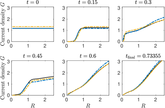
Figure 10: Nondimensional local current densities $G$ across particle sizes at selected times throughout a discharge. See caption and legend of Fig. 9.

The local surface concentrations and current densities as calculated from (55)-(56) for $R^{\mathrm{SPM}}=\bar{R}_{a}$ and $R^{\mathrm{SPM}}=\bar{R}_{c}$ are compared to the full MPM solution in Figs. 9 and 10. The approximations using either radius reproduce the actual concentrations and current densities surprisingly well for the whole range of particle sizes. Using $\bar{R}_{a}$ is most accurate near the beginning of the discharge and using $\bar{R}_{c}$ is most accurate towards the end, which is expected, since the SPM potential of each is most accurate at those times. Lastly, it is clear from Fig. 10 that current densities vary significantly across particle sizes, suggesting this is an important heterogeneous effect to capture to predict degradation. In particular, if, for example, the cell is cycled over a reduced range of states of charge, between 100% and 70% say, the smaller particles will be used disporportionately, with larger particles barely used at all in comparison, resulting in very different degradation rates.

4 Bimodal Particle-Size Distributions

In this section we will consider PSDs that are bimodal, i.e. have two distinct local maxima, such as those in Fig. 11$(a)$. These can occur in the manufacturing process from a single source (see [35]) or by the deliberate mixing of two unimodal distributions from different sources. This latter case of mixing is especially relevant to the case where two (or more) different electrode chemistries are mixed, which is becoming common in commercial lithium cells [12] and has been previously modelled [1]. Here we focus on modelling bimodal distributions of a single chemistry.

A bimodal number density $n(R)$ is modelled as the sum of two unimodal number densities, $n(R)=n_{1}(R)+n_{2}(R)$, where for each mode $n_{i}(R)$, $i=1,2$ we define area densities $a_{i}(R)$, volume densities $v_{i}(R)$ and the corresponding fraction densities $f_{n,i}(R)$, $f_{a,i}(R)$, and $f_{v,i}(R)$. We label the modes in order of increasing mean radii, $\bar{R}_{n,1}<\bar{R}_{n,2}$, and by choice of scaling we set $\bar{R}_{n,2}=1$. If the total particle number, area and volume of each mode are $n_{\mathrm{total},i}$, $a_{\mathrm{total},i}$, $v_{\mathrm{total},i}$, then

(57) $$n_{\mathrm{total}} =n_{\mathrm{total},1}+n_{\mathrm{total},2}, a_{\mathrm{total}} =a_{\mathrm{total},1}+a_{\mathrm{total},2}, 1/3 =v_{\mathrm{total},1}+v_{\mathrm{total},2},$$

where we recall that the total volume of the PSD has been scaled to be $1/3$. The distributions of the mixture are related to those of the individual modes via

(58) $$f_{n}(R) =\frac{n_{\mathrm{total},1}}{n_{\mathrm{total}}}f_{n,1}(R)+\frac{n_{\mathrm{total},2}}{n_{\mathrm{total}}}f_{n,2}(R),$$

and similarly for $f_{a}$ and $f_{v}$, where the rational coefficients lie between 0 and 1 and are interpreted as mixing parameters. If each $f_{n,i}$ is specified, fixing one coefficient determines the remainder. We choose to specify the proportion of the total active material volume contributed by mode 1, denoted $\delta_{1}=v_{\mathrm{total},1}/(1/3)=3v_{\mathrm{total},1}$.

4.1 Double particle model (DPM)

By taking the narrow limit $\sigma_{n,i}\to 0$ as in §3.2 for each mode simultaneously, we can use a single particle radius $R_{i}$ (i.e. any of the means defined in §3.1) to approximate each mode $i$ of the bimodal PSD, leading to a double particle model (DPM):

(59) $$\frac{\partial c_{i}}{\partial t} =\gamma\frac{1}{r^{2}}\frac{\partial}{\partial r}\left(r^{2}\frac{\partial c_{i}}{\partial r}\right), \text{for }0<r<R_{i},$$

(60) $$-\gamma\frac{\partial c_{i}}{\partial r} =\frac{1}{3}G(c_{i},\Delta\phi) \text{at }r=R_{i},$$

for $i\in\{1,2\}$, with $c_{i}=c_{\text{init}}$ initially and $c_{i}$ regular at $r=0$. These equations are coupled via the algebraic equation

(61) $$-I(t)=a_{\mathrm{total,}1}G(c_{s,1},\Delta\phi)+a_{\mathrm{total},2}G(c_{s,2},\Delta\phi),$$

where the area of each mode, in terms of the volume share $\delta_{1}$, is

(62) $$a_{\mathrm{total},1} =\frac{\delta_{1}}{R_{1}}, a_{\mathrm{total},2} =\frac{1-\delta_{1}}{R_{2}}.$$

4.1.1 Limit of large mode separation

The effects of bimodality are expected to be the most significant in the limit of large mode separation, $\epsilon=R_{1}/R_{2}\ll 1$. In taking the limit $\epsilon\to 0$, we need to decide how the volume share $\delta_{1}$ scales with $\epsilon$. There are several distinguished limits we could take, for example, $\delta_{1}(\epsilon)=O(\epsilon^{3})$, $O(\epsilon)$, and $O(1)$, corresponding to fixed particle number $n_{\mathrm{total},1}$, fixed surface area $a_{\mathrm{total},1}$, and fixed volume share, respectively. The first two cases give similar behaviour: the dynamics and cell potential are dominated by mode 2, with mode 1 providing a small correction of $O(\delta_{1})$. The last case, where $\delta_{1}=O(1)$ and the volume shares of both modes are comparable, has a more interesting behaviour and is presented below.

Writing $R_{1}=\epsilon R_{2},$ we rescale the domain in particle 1 via the transformation $\tilde{r}=r/\epsilon$, and substitute the regular expansions

(63) $$c_{i} =c_{i}^{(0)}+\epsilon c_{i}^{(1)}+O(\epsilon^{2}),\qquad i=1,2,$$

(64) $$G(c_{i,s},\Delta\phi) ={\mathcal{G}}_{i}^{(0)}+\epsilon{\mathcal{G}}_{i}^{(1)}+O(\epsilon^{2}),\qquad i=1,2,$$

(65) $$\Delta\phi =\Delta\Phi^{(0)}+\epsilon\Delta\Phi^{(1)}+O(\epsilon^{2}),$$

in powers of $\epsilon$ into (59)-(61). The first two orders in (61) give

(66) $${\mathcal{G}}_{1}^{(0)} =0,$$

(67) $${\mathcal{G}}_{1}^{(1)} =-R_{2}I(t)-(1-\delta_{1}){\mathcal{G}}_{2}^{(0)},$$

meaning at leading order particle 1 is in quasi-static equilibrium, with (66) rearranging to give $\Delta\Phi^{(0)}=U(c_{1,s}^{(0)})$, which can be used to eliminate $\Delta\Phi^{(0)}$. Since particle 1 is small, diffusion is fast there, $c^{(0)}_{1}=c^{(0)}_{1}(t)$, and the equations simplify as in §2.3. The analysis is straightforward, and the result is the following coupled system:

(68) $$\frac{\mathrm{d}c_{1}^{(0)}}{\mathrm{d}t} =I(t)+\frac{(1-\delta_{1})}{R_{2}}G(c_{2,s}^{(0)},U(c_{1}^{(0)})),$$

(69) $$\frac{\partial c_{2}^{(0)}}{\partial t} =\frac{\gamma}{r^{2}}\frac{\partial}{\partial r}\left(r^{2}\frac{\partial c_{2}^{(0)}}{\partial r}\right),\qquad\text{for }0<r<R_{2},$$

(70) $$-\gamma\frac{\partial c_{2}^{(0)}}{\partial r} =\frac{1}{3}G(c_{2}^{(0)},U(c_{1}^{(0)}))\qquad\text{at }r=R_{2}.$$

with $c_{1}^{(0)}=c_{\mathrm{init}}$, $c_{2}^{(0)}=c_{\text{init}}$ at $t=0$ and $c_{2}$ regular at $r=0$, where as usual $c_{2,s}^{(0)}$ is the surface value $c_{2}^{(0)}(R_{2},t)$. The reduced system (68)-(70) is computationally simpler than the DPM (59)-(62), and will be compared to the DPM for various size ratios $\epsilon$ in the next section.

4.2 Model results

In this section we present results of the full MPM (14)-(18) for bimodal PSDs, and the simpler two-particle models: the DPM (59)-(62) and its large-separation limit (68)-(70). We consider the constant current discharge of a graphite anode, with the parameters and numerical methods the same as for unimodal distributions in §3.3. For each mode $i=1,2$ of the PSD, the radius distribution $f_{n,i}(R)$ is a log-normal with mean $\bar{R}_{i}$ and variance $\sigma_{n,i}^{2}$.

4.2.1 Comparison of DPM to full bimodal PSD

To assess how well a DPM can reproduce the cell potential of the full MPM using the bimodal PSD, we choose the radii in the DPM to be the area-weighted means of each mode, $\bar{R}_{a,i}$, $i=1,2$. We choose the modes to have equal volume share so that $\delta_{1}=0.5$. The bimodal PSD, the mean radii, and resulting cell potentials are shown in Fig. 11. The DPM captures the smoothing of the steps very well. In contrast, an SPM at the mean $\bar{R}_{a}$ of the combined bimodal PSD cannot capture this effect. Futher, the DPM excellently reproduces the behaviour with C-rate, shown in Fig. 12, where the bimodal nature becomes more apparent as the C-rate increases.

These results justify the use of the DPM in place of the MPM for bimodal distributions in the remainder of this paper.

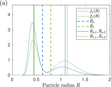
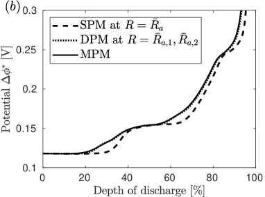
Figure 11: $(a)$ Bimodal PSD, showing area-weighted $f_{a}(R)$ and volume-weighted $f_{v}(R)$ distributions (solid), their means $\bar{R}_{a}$, $\bar{R}_{v}$ (dashed) and means of each mode (dotted). $(b)$ Cell potentials for MPM, DPM and SPM based on area-weighted means. Graphite, parameters $\mathcal{C}=1$, $\bar{R}_{n,1}=0.4$, $\bar{R}_{n,2}=1$, $\sigma_{a,i}=0.2\bar{R}_{a,i}$, $i=1,2$.

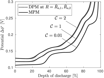
Figure 12: Cell potential for different C-rates $\mathcal{C}$ comparing DPM to MPM for full bimodal PSD, as in Fig. 11.

4.2.2 Effect of mode separation

Here we present the impact of mode separation in the DPM. We fix $\delta_{1}=0.5$ and vary the mode separation through $\epsilon=R_{1}/R_{2}$.

Results for $\epsilon=0.1,0.5,0.9$, as well as the asymptotic solution for large separation $\epsilon\ll 1$, are shown in Fig. 13. When $\epsilon=0.9$, both modes are close to the same size and thus the results are close to an SPM, and the fraction of current out of mode 2 (or 1) is approximately a half throughout the discharge—see Fig. 13$(b)$. As $\epsilon$ decreases, the separation increases, the total surface area of mode 1 increases, but its volume remains fixed. The result is a staggered depletion of both modes where the share of the current switches back and forth between the modes several times due to the “stepped” nature of graphite’s OCP. The effect on the potential is nontrivial—see Fig. 13$(a)$. As $\epsilon$ decreases, the plateaus are lowered (decreased reaction resistance) but the steps are reached earlier as mode 1 depletes faster.

The effects of mode separation are most extreme as $\epsilon\to 0$, where the asymptotic solution for large separation (dashed lines) is valid. This asymptotic solution agrees well with the solution for $\epsilon=0.1$, and provides a bound on the effects of bimodality presented here.

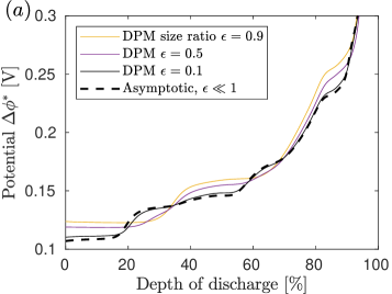
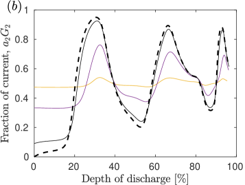
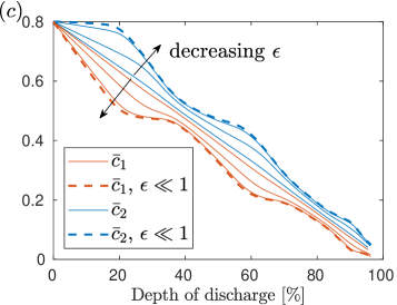
Figure 13: Results of the DPM with radii $R_{1}=\epsilon$, $R_{2}=1$, for various size ratios $\epsilon$. Solid lines are the DPM, dashed are the large separation limit (68)-(70). $(a)$ Potential; $(b)$ fraction of current or lithium flux for (larger) mode 2; $(c)$ particle-averaged concentrations for $\epsilon=0.1$, $0.5$, $0.9$. Graphite, parameters $\delta_{1}=0.5$, $\mathcal{C}=1$.

4.3 Comparison of model to experimental results for LiFePO₄

To further show that the DPM, given by (59)-(62), can capture behaviour observed in real cells, we compare the results of the model to experiments conducted on lithium iron phosphate (LiFePO₄) cathodes, a different electrode chemistry to that considered thus far in this paper. From two different sources of micro-particulate LiFePO₄ with different mean particle sizes, three cathodes were constructed consisting of (i) the source of larger particles only (MTI Corp.^®); (ii) the source of smaller particles only (Hydro-Québec^®); (iii) a (bimodal) mixture of both particle sizes, in approximately a 1:1 volume share. Coin half-cells for each type of cathode (denoted MTI, HQ and MTI+HQ) were constructed and, after minimal cycling, constant current discharges from 4 V (100% state of charge) to a cut-off value of 2.6 V were subsequently performed—see §D for full details of the experimental procedures.

To parametrise the model we take the electrochemical parameters and OCP from [29], the total volume fraction $v_{\mathrm{total}}$ and theoretical capacity (and hence the current density $C^{*}$ for a 1C discharge) from each experimental setup, and then fit the remaining parameters, i.e., the diffusion coefficient $D^{*}$, radii of each particle size $R_{1}^{*}<R_{2}^{*}$, and the volume share of the smaller particles in the mixture, $\delta_{1}$. The cases of only small or only large particles are taken by setting $\delta_{1}=1$ or $\delta_{1}=0$, respectively. The OCP from [29] was shifted slightly to match the voltage plateau as the C-rate approaches zero, at 3.409 V. The radii $R_{1}^{*}=120\,\mathrm{nm}$ and $R_{2}^{*}=400\,\mathrm{nm}$ were chosen to fit the centres of the voltage plateaus of the discharge curves for the small and large particles separately—comparable with the manufacturers’ estimates of average particle size, $100\,\mathrm{nm}$ and $500\,\mathrm{nm}$. The diffusion coefficient $D^{*}=1\times 10^{-17}\mathrm{m}^{2}\text{s}^{-1}$ was chosen to approximate the drop-off of the total discharged capacity with C-rate. Finally, for the mixture of sizes, the remaining parameter $\delta_{1}$ was chosen to fit the location of the voltage step, which is discussed shortly. The complete set of the fitted and experimentally determined parameters is given in Table 4.

Discharge voltage curves from the experiments and the model for C-rates from 0.1 up to 1 are shown in Fig. 14. When only one particle size is present, the agreement is only qualitative as one might expect since, in the model, electrolyte dynamics are neglected and we assume simple Fickian diffusion of lithium within the particles, whereas phase change models are more appropriate for LiFePO₄ [7, 42]. Thus, in particular, we cannot expect to capture the sloping tail at the end of discharge for higher C-rates, or the slope of the voltage plateau itself for lower C-rates (see [15]). Despite this the model is able to reproduce the step between two plateaus which occurs with the mixture of particles.

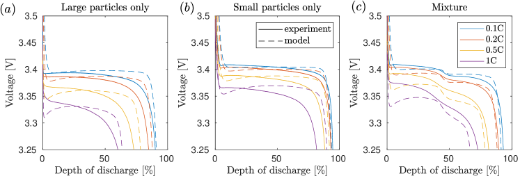
Figure 14: Voltage curves for constant current discharge of LiFePO₄ half-cells, comparing experiment to the model (DPM) for $(a)$ large particles only (MTI); $(b)$ small particles only (HQ); ($c$) mixture of small and large particles (MTI+HQ).

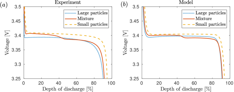
Figure 15: Voltage curves for constant current discharge of LiFePO₄ half-cells at 0.1C, with $(a)$ experimental results; $(b)$ model results (using DPM).

This phenomenon is best observed by showing results for all three electrodes on the same figure, and comparing the differences between model and experiment, as in Fig. 15. In either the model or the experiments, the cases of only smaller or larger particles have a single plateau, the former at a higher voltage due to the lower reaction resistance (higher active surface area). The mixture shows two plateaus with a step transition midway through the discharge. In the model this corresponds to intercalation of smaller particles first until saturation, followed by the larger particles (just as described for graphite in §4.2.2, but LiFePO₄ has only a single plateau). The plateaus of the mixture are lower than the corresponding ones for a single particle since the volume share is lower when in the mixture, but the applied current density is the same. These features are each present in the experiments, Fig. 15$(a)$. A more quantitative agreement could be achieved by extending the DPM to include electrolyte dynamics and phase-field physics, but that is outside the scope of this work.

Finally, we remark on the differences between this DPM and a similar DPM for spatially (bi-)layered electrodes presented in Richardson et al. [37]. In one scenario considered by [37], the electrode comprises particles of two distinct sizes, separated into two adjacent layers in the through-cell direction. In the asymptotic limit they consider (here corresponding to $\lambda\gg 1$), at leading order they derive a DPM of the form (59)-(62) with $G_{1}$ and $G_{2}$ elimitated, with the additional restriction that the concentrations on the surface of all particles, regardless of size, are identical for all time. The flux constraint (60) fixes this concentration, with the potential given by the equilibrium value $\Delta\phi(t)=U(c_{1,s})=U(c_{2,s})$. Since the double-plateau arises in our model from differing particle surface concentrations, it is not reproduced by the DPM of [37], which is more appropriate for materials whose OCP varies more strongly with state of charge.

5 Conclusions

In this paper we considered heterogeneity of the porous electrodes in lithium-ion batteries due to the presence of multiple particle sizes, in particular, particle-size distributions (PSDs). Using an electrochemical model of a half-cell valid for sufficiently low C-rates (less than one) where only lithium intercalation and diffusion within the spherical electrode particles are modelled, we presented a detailed investigation of the effect of the PSD on cell dynamics. We considered both unimodal and bimodal PSDs, and various approximations with single and double particle models (SPM and DPM) were evaluated for different choices of mean particle radii, of which there are several, with the aim of accurately reducing the model complexity.

For unimodal distributions, we investigated the effect of the spread of the PSD for the most common anode material, graphite, where the two chief effects found were: (1) smoothing of the cell potential throughout a constant current (dis)charge, a significant effect for graphite which has a “stepped” OCP; (2) reduction in usable capacity due to the heterogeneous distribution of lithium remaining (or absent) in different particle sizes at the end of a discharge (or charge). Results for SPMs for different choices of mean radii were compared to those for the full PSD, and asymptotic corrections to these models, consisting of three “correction particles”, were derived for narrow PSDs. An SPM can capture effect (2) for a wide range of operating conditions with a judicious choice of radius, and we systematically derive a new mean radius for this purpose, (35), which depends only on the PSD. An SPM cannot capture the smoothing effect, (1), but the asymptotic corrections for narrow PSDs can do so up to $\sigma_{n}^{*}/\bar{R}_{n}^{*}\lesssim 0.3$, a physically relevant range for graphite electrodes. The error in these corrected SPMs is localised temporally to when the state of the average particle passes a highly nonlinear section of the OCP. However, we showed that the highly heterogeneous internal states, e.g. concentrations and current densities, for all particle sizes can be accurately and efficiently predicted from an SPM after-the-fact, which may be useful for predicting nonuniform aging.

Next, we considered bimodal PSDs consisting of a mixture of two log-normal modes. The dynamics are found to be significantly different to that of a unimodal PSD but only if the two modes have a comparable volume share. Then, the cell potential for a full bimodal PSD is approximated excellently by a double particle model (DPM) using a single size to represent each mode. For graphite anodes, the introduction of a second mode has a nontrivial effect, with the “stepped” nature of the OCP resulting in a staggered (dis)charge where the share of the current switches between modes several times. An asymptotic limit of the DPM for large mode separation, eliminating the algebraic equation, gives an upper bound on these phenomena. Lastly, we presented experimental results for lithium iron phosphate cathodes with bimodal PSDs formed by mixing two unimodal PSDs of different means. The results showing a step transition between two voltage plateaus were reproduced by the DPM despite its mathematical simplicity and the assumption of linear Fickian solid-state diffusion, suggesting the phenomenon can be explained entirely by the bimodality of the PSD.

Appendix A Parameter values

The tables of parameter values used for the graphite anode and lithium iron phosphate cathode are given here. The dimensional and nondimensional parameters used for the graphite anode are given in Tables 2 and 3, respectively. Those for the lithium iron phosphate cathode used in the DPM to compare with experiment are given in Table 4.

Parameter	Description	Value
		[27, 25]
$R_{g}^{*}$	Universal gas constant $[\mathrm{J\,mol}^{-1}\mathrm{K}^{-1}]$	8.314472
$T^{*}$	Temperature $[\mathrm{K}]$	298.15
$F^{*}$	Faraday’s constant $[\mathrm{Cmol}^{-1}]$	96487
$c_{e}^{*}$	Li concentration in electrolyte $[\mathrm{mol}\,\mathrm{m}^{-3}]$	$10^{3}$
$L^{*}$	Electrode thickness $[\mathrm{m}]$	$100\times 10^{-6}$
$k^{*}$	Reaction rate $[\mathrm{A\,m}^{-2}(\mathrm{m}^{3}/\mathrm{mol})^{1.5}]$	$2\times 10^{-5}$
$c_{\mathrm{max}}^{*}$	Max. Li concentration in electrode $[\mathrm{mol}\,\mathrm{m}^{-3}]$	24983
$c_{\mathrm{init}}^{*}$	Initial Li concentration in electrode $[\mathrm{mol}\,\mathrm{m}^{-3}]$	$0.8c_{\mathrm{max}}^{*}$
$D^{*}$	Diffusivity of Li in electrode $[\mathrm{m}^{2}\mathrm{s}^{-1}]$	$3.9\times 10^{-14}$
$C^{*}$	Reference current density to discharge in 1hr $[\mathrm{A}\,\mathrm{m}^{-2}]$	24
$R_{\mathrm{typ}}^{*}$	Typical particle radius $[\mathrm{m}]$	$10^{-5}$
$a_{\mathrm{typ}}^{*}$	Typical surface area per volume $[\mathrm{m}^{-1}]$	$1.8\times 10^{-5}$
$v_{\mathrm{total}}$	Volume fraction of active material	0.6

Table 2: Parameter values for a graphite (LiC₆) anode [25, 27].

Nondimensional	Description	Definition	Value
parameter			[27, 25]
$\lambda$	1 V / thermal voltage	$F^{*}\Phi^{*}/(R_{g}^{*}T^{*})$	38.92
$\mathcal{C}$	C-rate	$I_{\text{typ}}^{*}/\text{C}^{*}$	(variable)
$k$	Nondimensional reaction rate	$\tau_{\text{d}}^{*}/\tau_{\text{reac}}^{*}$	$7.1103/\mathcal{C}$
$\gamma$	Nondimensional diffusivity	$\tau_{\text{d}}^{*}/\tau_{\mathrm{diff}}^{*}$	$2.3503/\mathcal{C}$
$c_{\mathrm{init}}$	Initial Li concentration	$c_{\mathrm{init}}^{*}/c_{\mathrm{max}}^{*}$	0.8

Table 3: Nondimensional parameter values for a graphite (LiC₆) anode. The dependence of each parameter on the C-rate, $\mathcal{C}$, is shown explicitly.

Parameter	Description	Experiments
		Small particles	Large particles	Mixture
		(HQ)	(MTI)	(HQ+MTI)
$k^{*}$	Reaction rate $[\mathrm{A\,m}^{-2}(\mathrm{m}^{3}/\mathrm{mol})^{1.5}]$	$1.35\times 10^{-7}$ [29]
$c_{\mathrm{max}}^{*}$	Max. Li concentration in electrode $[\mathrm{mol}\,\mathrm{m}^{-3}]$	$22806$ [29]
$D^{*}$	Diffusivity of Li in electrode $[\mathrm{m}^{2}\mathrm{s}^{-1}]$	$1\times 10^{-17}$ (fit)
$R_{1}^{*}$	Particle radius of small particles $[\mathrm{m}]$	$120\times 10^{-9}$ (fit)	-	$120\times 10^{-9}$
$R_{2}^{*}$	Particle radius of large particles $[\mathrm{m}]$	-	$400\times 10^{-9}$ (fit)	$400\times 10^{-9}$
$\delta_{1}$	Volume share of small particles	$1$	$0$	$0.4$ (fit)
$v_{\mathrm{total}}$	Volume fraction of active material	$0.3272$	$0.3719$	$0.3492$
$C^{*}$	Current density for 1C $[\mathrm{A}\,\mathrm{m}^{-2}]$	$13.60$	$14.32$	$13.66$

Table 4: Parameter values for LiFePO₄ cathode used in the DPM (59)-(62). Those found by fitting to experiment are indicated.

Appendix B Narrow distributions: Asymptotic correction for other mean radii

To develop the first correction term to an SPM with particle radius $\bar{R}_{i}$, where $i=n,a,v$, we express the problem in terms of $f_{i}(R)$. We can express $a(R)$, which appears in the integral constraint (18), in terms of any of the radius, area-weighted or volume-weighted distributions via

(71) $$a(R)=\begin{dcases}\frac{1}{m_{n,3}}R^{2}f_{n}(R)&\text{(radius)}\\ \frac{1}{\bar{R}_{a}}f_{a}(R)&\text{(area-weighted)}\\ \frac{f_{v}(R)}{R}&\text{(volume-weighted)}\end{dcases}$$

The standard deviations $\sigma_{i}$ are a measure of the spread of each distribution and we can consider the narrow distribution limit of each by taking $\sigma_{i}\to 0$ while fixing $\bar{R}_{i}$. Of course, the distributions are not independent of each other, and their moments, $m_{i,j}$, are related via

(72) $$m_{a,j} =\frac{m_{n,j+2}}{m_{n,2}}, j =1,2,...$$

(73) $$m_{v,j} =\frac{m_{a,j+1}}{m_{a,1}}=\frac{m_{n,j+3}}{m_{n,3}}, j =1,2,...$$

so that the means and variances satisfy

(74) $$\bar{R}_{a} =m_{a,1}=\frac{m_{n,3}}{m_{n,2}}, \sigma_{a}^{2} =m_{a,2}-m_{a,1}^{2}=\frac{m_{n,4}}{m_{n,2}}-\left(\frac{m_{n,3}}{m_{n,2}}\right)^{2}$$

(75) $$\bar{R}_{v} =\bar{R}_{a}\left(1+\frac{\sigma_{a}^{2}}{\bar{R}_{a}^{2}}\right), \sigma_{v}^{2} =\sigma_{a}^{2}+\frac{\sigma_{a}^{3}}{\bar{R}_{a}}\tilde{\mu}_{3,a}-\frac{\sigma_{a}^{4}}{\bar{R}_{a}^{2}},$$

where $\tilde{\mu}_{3,a}=\int_{0}^{\infty}(R-\bar{R}_{a})^{3}f_{a}\mathrm{d}R/\sigma_{a}^{3}$ is the coefficient of skewness (standardised third central moment) representing the asymmetry of $f_{a}$ about its mean. It follows from the above relations that if $\sigma_{i}\to 0$ for any $i$, then $\sigma_{n}\sim\sigma_{a}\sim\sigma_{v}\to 0$, and the means are all within $O(\sigma_{i}^{2})$ of each other, e.g., $\bar{R}_{v}=\bar{R}_{a}+O(\sigma_{a}^{2})=\bar{R}_{n}+O(\sigma_{n}^{2})$.

In §3.2 of the paper, the asymptotic limit of narrow distributions for fixed area-weighted mean radius $\bar{R}_{a}$ was given in detail. Here we give the corresponding results for fixed mean radius $\bar{R}_{n}$ and fixed volume-weighted mean radius $\bar{R}_{v}$.

B.1 Mean radius

The integral constraint written in terms of the radius distribution $f_{n}(R)$, with mean $\bar{R}_{n}$ and variance $\sigma_{n}^{2}$, is

(76) $$-I(t)=\frac{1}{m_{n,3}}\int_{0}^{\infty}R^{2}f_{n}(R)G(c_{s}(t;R),\Delta\phi(t))\mathrm{d}R.$$

The analysis for $\sigma_{n}\ll 1$ follows similarly to that of the area-weighted distribution in §3.2 of the paper, but with $G$ replaced by $R^{2}G$ in the integral, and with a prefactor of $1/m_{n,3}$. At $O(\sigma_{n}^{0})$ and $O(\sigma_{n}^{2})$ we find

(77) $$-I(t) =\frac{1}{\bar{R}_{n}}G_{n}^{(0)},$$

(78) $$0 =\bar{R}_{n}^{2}G_{n}^{(2)}+G_{n}^{(0)}+\bar{R}_{n}\left(\frac{\partial G^{(0)}}{\partial R}\right)_{n}+\frac{1}{2}\bar{R}_{n}^{2}\left(\frac{\partial^{2}G^{(0)}}{\partial R^{2}}\right)_{n}-\frac{m_{n,3}^{(2)}}{\bar{R}_{n}^{3}}G_{n}^{(0)},$$

where we have expanded also $m_{n,3}$ (it depends on $\sigma_{n}$) so that

(79) $$\frac{1}{m_{n,3}} =\frac{1}{m_{n,3}^{(0)}+\sigma_{n}^{2}m_{n,3}^{(2)}+\cdots}=\frac{1}{\bar{R}_{n}^{3}}-\sigma_{n}^{2}\frac{m_{n,3}^{(2)}}{\bar{R}_{n}^{6}}+\cdots.$$

For a log-normal $m_{n,3}^{(2)}=3\bar{R}_{n}$. At leading order, (77) gives the SPM (27)-(31) at radius $R=\bar{R}_{n}$, with solution $c_{n}^{(0)}$ and $\Delta\phi^{(0)}$, say.

At $O(\sigma_{n}^{2})$ the correction to the flux $G_{n}^{(2)}$ depends on both $\partial G/\partial R$ and $\partial^{2}G/\partial R^{2}$. Then $\partial^{2}G/\partial R^{2}$ is calculated as in §3.2 (with $\bar{R}_{a}$ replaced by $\bar{R}_{n}$), while $\partial G/\partial R$ can be calculated similarly using

(80) $$\left(\frac{\partial G^{(0)}}{\partial R}\right)_{n}=\begin{dcases}\left(\frac{\partial G^{(0)}}{\partial c}\right)_{n}\left(\frac{\partial c^{(0)}}{\partial R}\right)_{n}&\gamma=\infty,\\ \frac{G(c_{n,+,s}^{(0)},\Delta\phi^{(0)})-G(c_{n,-,s}^{(0)},\Delta\phi^{(0)})}{2\Delta R}+O(\Delta R^{2})&\text{$\gamma\neq\infty$}.\end{dcases}$$

Then (51)-(54) still hold (with $\bar{R}_{a}$ and $G_{a}^{(2)}$ replaced by $\bar{R}_{n}$ and $G_{n}^{(2)}$).

B.2 Volume-weighted mean radius

The integral constraint written in terms of the volume-weighted distribution $f_{v}(R)$, with mean $\bar{R}_{v}$ and variance $\sigma_{v}^{2}$, is

(81) $$-I(t)=\int_{0}^{\infty}f_{v}(R)\frac{G(c_{s}(t;R),\Delta\phi(t))}{R}\mathrm{d}R.$$

The analysis for $\sigma_{v}\ll 1$ follows similarly to that of the area-weighted distribution in section 3.2, but with $G$ replaced by $G/R$ in the integral. At $O(\sigma_{n}^{0})$ and $O(\sigma_{n}^{2})$ we find

(82) $$-I(t) =\frac{1}{\bar{R}_{v}}G_{v}^{(0)},$$

(83) $$0 =\frac{1}{\bar{R}_{v}}G_{v}^{(2)}+\frac{1}{2}\left[\frac{2}{\bar{R}_{v}^{3}}G_{v}^{(0)}-\frac{2}{\bar{R}_{v}^{2}}\left(\frac{\partial G^{(0)}}{\partial R}\right)_{v}+\frac{1}{\bar{R}_{v}}\left(\frac{\partial^{2}G^{(0)}}{\partial R^{2}}\right)_{v}\right].$$

At leading order, (82) results in the SPM at radius $R=\bar{R}_{v}$, with solution $c_{v}^{(0)}$ and $\Delta\phi^{(0)}$, say.

At $O(\sigma_{v}^{2})$, (83) gives the correction $G_{v}^{(2)}$ to the flux. Then $\partial^{2}G/\partial R^{2}$ and $\partial G/\partial R$ are calculated as in §3.2 (and (80) above), now at the radius $\bar{R}_{v}$. Given $G_{v}^{(0)}$, (51)-(54) still hold (with $\bar{R}_{a}$ and $G_{a}^{(2)}$ replaced by $\bar{R}_{v}$ and $G_{v}^{(2)}$).

Appendix C Expressions for $\partial G/\partial c$ and $\partial^{2}G/\partial c^{2}$

In this section we give expressions for the derivatives of the (nondimensional) surface lithium flux with respect to concentration, for use in §3.2. Differentiating the expression (17) for $G(c,\Delta\phi)$ with respect to $c$,

(84) $$\frac{\partial G}{\partial c} =\frac{g^{\prime}}{g}G-\frac{\lambda}{2}U^{\prime}(c)\sqrt{g^{2}+G^{2}},$$

(85) $$\frac{\partial^{2}G}{\partial c^{2}} =\frac{g^{\prime\prime}}{g}G+\frac{\lambda^{2}}{4}(U^{\prime}(c))^{2}G-\frac{\lambda}{2}\sqrt{g^{2}+G^{2}}\left[\frac{2g^{\prime}(c)}{g(c)}U^{\prime}(c)+U^{\prime\prime}(c)\right],$$

where

$$g(c) =kc^{1/2}(1-c^{1/2}), g^{\prime}(c) =\frac{k^{2}\left(\frac{1}{2}-c\right)}{g}, g^{\prime\prime}(c) =-\frac{\left(k^{2}-(g^{\prime})^{2}\right)}{g},$$

and primes denote $\mathrm{d}/\mathrm{d}c$.

Appendix D Experimental methods

In this section we give the experimental details and methods used to construct the LiFePO₄ half-cells referred to in §4.3.

Electrodes were spray deposited from suspensions of LiFePO₄ with component ratios of 87:3:10 of active material (AM), carboxymethyl cellulose (CMC), and carbon black (CB), respectively. Slurry mixtures of the MTI Corp.^® and and HQ (Hydro-Québec^®) sources of LiFePO₄ were prepared at 350 rpm using 10 mm zirconia balls and a two step mixing process: (1) CB and 2.5 wt. % CMC aqueous solution were mixed for 15 min and then (2) LiFePO₄ and deionised (DI) water were added to the CB-based slurry and mixed for a further 15 min. In step (2), DI water was added until the slurry reached a mass concentration of 40 wt. %. The resulting slurry was then diluted to a 1 wt. % solid concentration using DI water and agitated on a magnetic stirrer for 2 hours before spray deposition. For the mixed electrode, MT+HQ, a slurry of HQ and MTI was ball milled, with a HQ:MTI ratio of 47.5:52.5 wt. %.

Spray deposition of suspensions was performed with a pneumatic spray nozzle mounted on an X-Y gantry over a heated vacuum chuck. The temperature of the substrate was 130 ^∘C, the flow rate of the suspension was 4.5 ml/min and the atomisation pressure was 0.4 bar. MTI, HQ and HQ+MTI mixed suspensions were spray deposited until an electrode thickness of 80 $\mu$m was deposited. After deposition, the coated aluminium foils were removed from the heated substrate, calendered and moved to a vacuum oven at 130 ^∘C overnight before cell assembly.

Cells were assembled in a glove box with an Ar atmosphere of $<0.1$ ppm H₂O and $<0.1$ ppm O₂. Foil electrodes were assembled with the following components placed one after another in the centre of a CR2032 coin cell cup (MTI Corp.): (1) the working electrode, (2) 75 $\mu$l of 1 molar LiPF₆ in EC:DMC=1:1 (by volume) electrolyte (Sigma Aldrich), (3) a glass fibre separator (0.5mm thick, 18mm diameter, Watson Marlow), (4) 75 $\mu$l of 1 molar LiPF₆ in EC:DMC=1:1 (by volume) electrolyte, (5) a pre-cut Li chip (0.6 mm thick, 15 mm diameter, MTI Corp.), (6) a stainless steel spacer (1mm thick, 15.5mm diameter), (7) a stainless steel wave spring (0.3 mm thick, MTI Corp.) and (8) a CR2032 coin cell cap (MTI Corp.). The assembled cells were crimped at 0.08 T (arbitrary units) using an MTI MSK-160E Electric Crimper and cleaned with ethanol after removal from the glove box. Cells were allowed to rest for at least 20 hours before initial cycling was performed.

References

- [1] P. Albertus, J. Christensen, and J. Newman, Experiments on and modeling of positive electrodes with multiple active materials for lithium-ion batteries, J. Elec. Soc., 156 (2009), pp. A606–A618, https://doi.org/10.1149/1.3129656.
- [2] T. Allen, Particle Size Measurement, Chapman & Hall, 4th ed., 1992.
- [3] L. Bayvel and Z. Orzechowski, Liquid Atomization, Taylor & Francis, 1st ed., 1993.
- [4] A. M. Bizeray, J. Kim, S. R. Duncan, and D. A. Howey, Identifiability and parameter estimation of the single particle lithium-ion battery model, IEEE T. Contr. Syst. T., 27 (2019), pp. 1862–1877, https://doi.org/10.1109/TCST.2018.2838097.
- [5] G. E. Blomgren, The development and future of lithium ion batteries, J. Elec. Soc., 164 (2017), pp. A5019–A5025, https://doi.org/10.1149/2.0251701jes.
- [6] H. Buqa, A. Würsig, D. Goers, L. J. Hardwick, M. Holzapfel, P. Novák, F. Krumeich, and M. Spahr, Behaviour of highly crystalline graphites in lithium-ion cells with propylene carbonate containing electrolytes, J. Power Sources, 146 (2005), pp. 134 – 141, https://doi.org/10.1016/j.jpowsour.2005.03.106. Selected papers pressented at the 12th International Meeting on Lithium Batteries.
- [7] G. Chen, X. Song, and T. Richardson, Electron microscopy study of the LiFePO4 to FePO4 phase transition, Electrochem. Solid St., 9 (2006), pp. A295–A298, https://doi.org/10.1149/1.2192695.
- [8] C. Cheng, R. Drummond, S. R. Duncan, and P. S. Grant, Micro-scale graded electrodes for improved dynamic and cycling performance of li-ion batteries, J. Power Sources, 413 (2019), pp. 59 – 67, https://doi.org/https://doi.org/10.1016/j.jpowsour.2018.12.021.
- [9] R. Darling and J. Newman, Modeling a porous intercalation electrode with two characteristic particle sizes, J. Elec. Soc., 144 (1997), p. 4201, https://doi.org/10.1149/1.1838166.
- [10] M. Doyle, T. M. Fuller, and J. Newman, Modeling of galvanostatic charge and discharge of the lithium/polymer/insertion cell., J. Elec. Soc., 140 (1993), pp. 1526–1533.
- [11] T. Drezen, N.-H. Kwon, P. Bowen, I. Teerlinck, M. Isono, and I. Exnar, Effect of particle size on LiMnPO4 cathodes, J. Power Sources, 174 (2007), pp. 949 – 953, https://doi.org/10.1016/j.jpowsour.2007.06.203. 13th International Meeting on Lithium Batteries.
- [12] M. Dubarry, C. Truchot, M. Cugnet, B. Y. Liaw, K. Gering, S. Sazhin, D. Jamison, and C. Michelbacher, Evaluation of commercial lithium-ion cells based on composite positive electrode for plug-in hybrid electric vehicle applications. Part I: Initial characterizations, J. Power Sources, 196 (2011), pp. 10328 – 10335, https://doi.org/10.1016/j.jpowsour.2011.08.077.
- [13] M. Farkhondeh and C. Delacourt, Mathematical modeling of commercial LiFePO4 electrodes based on variable solid-state diffusivity, J. Elec. Soc., 159 (2011), pp. A177–A192, https://doi.org/10.1149/2.073202jes.
- [14] M. Farkhondeh, M. Safari, M. Pritzker, M. Fowler, T. Han, J. Wang, and C. Delacourt, Full-range simulation of a commercial LiFePO4 electrode accounting for bulk and surface effects: A comparative analysis, J. Elec. Soc., 161 (2014), pp. A201–A212, https://doi.org/10.1149/2.094401jes.
- [15] T. R. Ferguson and M. Z. Bazant, Phase transformation dynamics in porous battery electrodes, Electrochim. Acta, 146 (2014), pp. 89 – 97, https://doi.org/10.1016/j.electacta.2014.08.083.
- [16] G. T.-K. Fey, Y. G. Chen, and H.-M. Kao, Electrochemical properties of LiFePO4 prepared via ball-milling, J. Power Sources, 189 (2009), pp. 169 – 178, https://doi.org/10.1016/j.jpowsour.2008.10.016.
- [17] A. A. Franco, Multiscale modelling and numerical simulation of rechargeable lithium ion batteries: concepts, methods and challenges, RSC Advances, 3 (2013), pp. 13027–13058, https://doi.org/10.1039/C3RA23502E.
- [18] T. F. Fuller, M. Doyle, and J. Newman, Simulation and optimization of the dual lithium ion insertion cell, J. Elec. Soc., 141 (1994), pp. 1–10, https://doi.org/10.1149/1.2054684.
- [19] D. Goers, M. E. Spahr, A. Leone, W. Märkle, and P. Novák, The influence of the local current density on the electrochemical exfoliation of graphite in lithium-ion battery negative electrodes, Electrochim. Acta, 56 (2011), pp. 3799 – 3808, https://doi.org/10.1016/j.electacta.2011.02.046.
- [20] A. Jokar, B. Rajabloo, M. Désilets, and M. Lacroix, Review of simplified pseudo-two-dimensional models of lithium-ion batteries, J. Power Sources, 327 (2016), pp. 44 – 55, https://doi.org/10.1016/j.jpowsour.2016.07.036.
- [21] H. Kondo, T. Sasaki, P. Barai, and V. Srinivasan, Comprehensive study of the polarization behavior of LiFePO4electrodes based on a many-particle model, J. Elec. Soc., 165 (2018), pp. A2047–A2057, https://doi.org/10.1149/2.0181810jes.
- [22] P. B. Kowalczuk and J. Drzymala, Physical meaning of the sauter mean diameter of spherical particulate matter, Particul. Sci. Technol., 34 (2016), pp. 645–647, https://doi.org/10.1080/02726351.2015.1099582.
- [23] M. I. Limited, A basic guide to particle characterization. https://www.cif.iastate.edu/sites/default/files/uploads/Other_Inst/Particle%20Size/Particle%20Characterization%20Guide.pdf, Accessed 2019.
- [24] M. M. Majdabadi, S. Farhad, M. Farkhondeh, R. A. Fraser, and M. Fowler, Simplified electrochemical multi-particle model for LiFePO4 cathodes in lithium-ion batteries, J. Power Sources, 275 (2015), pp. 633 – 643, https://doi.org/10.1016/j.jpowsour.2014.11.066.
- [25] S. G. Marquis, V. Sulzer, R. Timms, C. P. Please, and S. J. Chapman, An asymptotic derivation of a single particle model with electrolyte, J. Elec. Soc., 166 (2019), p. A3693, https://doi.org/10.1149/2.0341915jes.
- [26] J. P. Meyers, M. Doyle, R. M. Darling, and J. Newman, The impedance response of a porous electrode composed of intercalation particles, J. Elec. Soc., 147 (2000), pp. 2930–2940, https://doi.org/10.1149/1.1393627.
- [27] S. Moura, fastdfn. https://github.com/scott-moura/fastDFN, 2016.
- [28] S. J. Moura, F. B. Argomedo, R. Klein, A. Mirtabatabaei, and M. Krstic, Battery state estimation for a single particle model with electrolyte dynamics, IEEE Transactions on Control Systems Technology, 25 (2017), pp. 453–468, https://doi.org/10.1109/TCST.2016.2571663.
- [29] I. R. Moyles, M. G. Hennessy, T. G. Myers, and B. R. Wetton, Asymptotic reduction of a porous electrode model for lithium-ion batteries, SIAM J. Appl. Math., 79 (2019), pp. 1528–1549, https://doi.org/10.1137/18M1189579.
- [30] J. Newman, Fortran programs for simulation of electrochemical systems, dualfoil.f program for lithium battery simulation. www.cchem.berkeley.edu/jsngrp/fortran.html, 2004.
- [31] J. Newman and K. E. Thomas-Alyea, Electrochemical Systems, John Wiley & Sons, 2012.
- [32] G. Ning and B. N. Popov, Cycle life modeling of lithium-ion batteries, J. Elec. Soc., 151 (2004), pp. A1584–A1591, https://doi.org/10.1149/1.1787631.
- [33] H. E. Perez, X. Hu, and S. J. Moura, Optimal charging of batteries via a single particle model with electrolyte and thermal dynamics., in American Control Conference (ACC), IEEE, 2016, pp. 4000–4005.
- [34] D. Ramkrishna, Population Balances: Theory and Applications to Particulate Systems in Engineering, Academic Press, 2000.
- [35] A. J. R. Rennie, V. L. Martins, R. M. Smith, and P. J. Hall, Influence of particle size distribution on the performance of ionic liquid-based electrochemical double layer capacitors, Scientific Reports, 6 (2016), p. 22062.
- [36] G. Richardson, G. Denuault, and C. P. Please, Multiscale modelling and analysis of lithium-ion battery charge and discharge, J. Eng. Math., 72 (2012), pp. 41–72, https://doi.org/10.1007/s10665-011-9461-9.
- [37] G. Richardson, I. Korotkin, R. R. M. Castle, and J. M. Foster, Generalised single particle models for high-rate operation of graded lithium-ion electrodes: systematic derivation and validation, Electrochim. Acta, 339 (2020), p. 135862, https://doi.org/10.1016/j.electacta.2020.135862.
- [38] F. Röder, S. Sonntag, D. Schröder, and U. Krewer, Simulating the impact of particle size distribution on the performance of graphite electrodes in lithium-ion batteries, Energy Technology, 4 (2016), pp. 1588–1597, https://doi.org/10.1002/ente.201600232.
- [39] J. Song and M. Z. Bazant, Effects of nanoparticle geometry and size distribution on diffusion impedance of battery electrodes, J. Elec. Soc., 160 (2013), pp. A15–A24, https://doi.org/10.1149/2.023301jes.
- [40] V. Srinivasan and J. Newman, Discharge model for the lithium iron-phosphate electrode, J. Elec. Soc., 151 (2004), p. A1517, https://doi.org/10.1149/1.1785012.
- [41] S. T. Taleghani, B. Marcos, K. Zaghib, and G. Lantagne, A study on the effect of porosity and particles size distribution on li-ion battery performance, J. Elec. Soc., 164 (2017), pp. E3179–E3189, https://doi.org/10.1149/2.0211711jes.
- [42] M. Tang, W. Carter, and Y.-M. Chiang, Electrochemically driven phase transitions in insertion electrodes for lithium-ion batteries: Examples in lithium metal phosphate olivines, Annu. Rev. Mat. Res., 40 (2010), pp. 501–529, https://doi.org/10.1146/annurev-matsci-070909-104435.
- [43] D. Wang and L.-S. Fan, 2 - Particle characterization and behavior relevant to fluidized bed combustion and gasification systems, in Fluidized Bed Technologies for Near-Zero Emission Combustion and Gasification, F. Scala, ed., Woodhead Publishing Series in Energy, Woodhead Publishing, 2013, pp. 42 – 76, https://doi.org/10.1533/9780857098801.1.42.
- [44] J. Yi, U. S. Kim, C. B. Shin, T. Han, and S. Park, Three-dimensional thermal modeling of a lithium-ion battery considering the combined effects of the electrical and thermal contact resistances between current collecting tab and lead wire, J. Elec. Soc., 160 (2013), pp. A437–A443, https://doi.org/10.1149/2.039303jes.
- [45] T. G. Zavalis, M. Klett, M. H. Kjell, M. Behm, R. W. Lindström, and G. Lindbergh, Aging in lithium-ion batteries: Model and experimental investigation of harvested LiFePO4 and mesocarbon microbead graphite electrodes., Electrochim. Acta, (2013), pp. 335–348, https://doi.org/10.1016/j.electacta.2013.05.081.
- [46] G. Zubi, R. Dufo-López, M. Carvalho, and G. Pasaoglu, The lithium-ion battery: State of the art and future perspectives, Renew. Sust. Energ. Rev., 89 (2018), pp. 292–308, https://doi.org/10.1016/j.rser.2018.03.00.