The multivariate tail-inflated normal distribution
and its application in finance

Abstract

This paper introduces the multivariate tail-inflated normal (MTIN) distribution, an elliptical heavy-tails generalization of the multivariate normal (MN). The MTIN belongs to the family of MN scale mixtures by choosing a convenient continuous uniform as mixing distribution. Moreover, it has a closed-form for the probability density function characterized by only one additional “inflation” parameter, with respect to the nested MN, governing the tail-weight. The first four moments are also computed; interestingly, they always exist and the excess kurtosis can assume any positive value. The method of moments and maximum likelihood (ML) are considered for estimation. As concerns the latter, a direct approach, as well as a variant of the EM algorithm, are illustrated. The existence of the ML estimates is also evaluated. Since the inflation parameter is estimated from the data, robust estimates of the mean vector and covariance matrix of the nested MN distribution are automatically obtained by down-weighting. Simulations are performed to compare the estimation methods/algorithms and to investigate the ability of AIC and BIC to select among a set of candidate elliptical models. For illustrative purposes, the MTIN distribution is finally fitted to multivariate financial data where its usefulness is also shown in comparison with other well-established multivariate elliptical distributions.

Keywords: Elliptical distributions, Financial applications, Heavy-tailed distributions, Maximum likelihood, Scale mixtures, Uniform distribution

1 Introduction

Statistical inference dealing with continuous multivariate data is commonly focused on the multivariate normal (MN) distribution, with mean vector $\boldsymbol{\mu}$ and covariance matrix $\boldsymbol{\Sigma}$, due to its computational and theoretical convenience. However, for many real phenomena, the tails of this distribution are lighter than required. This is often due to the presence of mild outliers (Ritter, 2015, p. 4). Outliers are defined as “mild”, with respect to the MN distribution (which is the reference distribution), when they do not really deviate from the MN and are not strongly outlying, but rather they produce an overall distribution that is too heavy-tailed to be modeled by the MN (Mazza and Punzo, 2020, Morris et al., 2019, and Punzo and Tortora, 2019); for a discussion about the concept of reference (or target) distribution, see Davies and Gather (1993). Therefore, mild outliers can be modeled by means of a heavy-tailed elliptically symmetric (or elliptically contoured or, simply, elliptical) distribution embedding the MN distribution as a special case (Ritter, 2015, p. 79).

A classical way to define such a larger model is by means of the MN scale mixture (also known as MN variance mixture); it is a finite/continuous mixture of MN distributions on $\boldsymbol{\Sigma}$ obtained via a convenient discrete/continuous mixing distribution with positive support. The MN scale mixture simply alters the tail behavior of the MN distribution while leaving the resultant distribution elliptically contoured. This is made possible by the additional parameters of the mixing distribution which, in the scale mixture, govern the deviation from normality in terms of tail weight. Regardless of the mixing distribution considered, expressing a multivariate elliptical distribution as a MN scale mixture enables (among other): natural/efficient computation of the maximum likelihood (ML) estimates via expectation-maximization (EM) based algorithms (Lange and Sinsheimer, 1993 and Balakrishnan et al., 2009), robust ML estimation of the parameters $\boldsymbol{\mu}$ and $\boldsymbol{\Sigma}$ based on down-weighting of mild outliers (Peel and McLachlan, 2000, Punzo and McNicholas, 2016, and Farcomeni and Punzo, 2019), and efficient Monte Carlo calculations (Relles, 1970, Andrews and Mallows, 1974, Efron and Olshen, 1978 and Choy and Chan, 2008). Moreover, robustness studies have often used MN scale mixtures for simulation and in the analysis of outlier models; see West (1984, 1987) and the references therein.

The MN scale mixture family includes many classical distributions, such as the multivariate $t$ (M$t$; Lange et al., 1989 and Kotz and Nadarajah, 2004), obtained by using a convenient gamma as mixing distribution, the multivariate contaminated normal (MCN) of Tukey (1960, see also , ), defined under a convenient Bernoulli mixing distribution (see, e.g., Yamaguchi, 2004 and Punzo et al., 2020), and the multivariate symmetric generalized hyperbolic (MSGH; McNeil et al., 2005) obtained if a generalized inverse Gaussian is considered as mixing distribution.

In the present paper, we add a new member to the MN scale mixture family: the multivariate tail-inflated normal (MTIN) distribution. It is obtained by using a convenient continuous uniform as mixing distribution. In Section 2.1 we show that the proposed distribution has a closed-form probability density function (pdf) which is characterized by a single additional parameter, with respect to $\boldsymbol{\mu}$ and $\boldsymbol{\Sigma}$ of the nested MN, governing the tail weight. We also make explicit the representations of the MTIN distribution as MN scale mixture (Section 2.2.1) and as elliptical distribution (Section 2.2.2). In Section 2.3 we provide the first four moments of the MTIN distribution, which are those of practical interest (see also Appendix B). We estimate the parameters by the method of moments (Appendix C) and maximum likelihood (ML; Section 3); for the latter, we illustrate two alternative algorithms/methods to obtain these estimates (a direct approach in Section 3.1 and an ECME algorithm in Section 3.2). Always for the ML method, in Section 4 we discuss the existence of the estimates. The ECME algorithm allows us to highlights how the ML estimates of $\boldsymbol{\mu}$ and $\boldsymbol{\Sigma}$ are robust in the sense that mild outliers are down-weighted in the computation of these parameters (see Section 5 for details). Two simulated data analyses are designed to compare the estimation methods discussed above in terms of parameter recovery and computational time required (Section 6.1), and to evaluate the appropriateness of AIC and BIC in selecting among a set of candidate elliptical models that can be considered as natural competitors of our MTIN distribution (Section 6.2). At last, we illustrate the proposed model by analyzing financial multivariate data related to four of the publicly owned companies considered by the Dow Jones index (Section 7); here, we also compare the performance of the MTIN distribution with other heavy-tailed elliptical distributions which are well-known in the financial literature. We conclude the paper with a brief discussion in Section 8.

2 Multivariate tail-inflated normal distribution

2.1 Probability density function

Definition 2.1 (Probability density function).

A $d$-dimensional random vector $\boldsymbol{X}$ is said to have a $d$-variate tail-inflated normal distribution with mean vector $\boldsymbol{\mu}\in{}^{d}$, $d\times d$ scale matrix $\boldsymbol{\Sigma}$, and inflation parameter $\theta\in\left(0,1\right)$, in symbols $\boldsymbol{X}\sim\mathcal{TIN}_{d}\left(\boldsymbol{\mu},\boldsymbol{\Sigma},\theta\right)$, if its pdf is given by

$$f_{\text{TIN}}\left(\boldsymbol{x};\boldsymbol{\mu},\boldsymbol{\Sigma},\theta\right)=\frac{2\pi^{-\frac{d}{2}}\left|\boldsymbol{\Sigma}\right|^{-\frac{1}{2}}}{\theta\left[\delta\left(\boldsymbol{x};\boldsymbol{\mu},\boldsymbol{\Sigma}\right)\right]^{\left(\frac{d}{2}+1\right)}}\left[\Gamma\left(\frac{d}{2}+1,(1-\theta)\frac{\delta\left(\boldsymbol{x};\boldsymbol{\mu},\boldsymbol{\Sigma}\right)}{2}\right)-\Gamma\left(\frac{d}{2}+1,\frac{\delta\left(\boldsymbol{x};\boldsymbol{\mu},\boldsymbol{\Sigma}\right)}{2}\right)\right],$$ (1)

where $\Gamma\left(\cdot,\cdot\right)$ is the upper incomplete gamma function, $\left|\cdot\right|$ is the determinant, and $\delta\left(\boldsymbol{x};\boldsymbol{\mu},\boldsymbol{\Sigma}\right)=\left(\boldsymbol{x}-\boldsymbol{\mu}\right)^{\prime}\boldsymbol{\Sigma}^{-1}\left(\boldsymbol{x}-\boldsymbol{\mu}\right)$ denotes the squared Mahalanobis distance between $\boldsymbol{x}$ and $\boldsymbol{\mu}$ (with $\boldsymbol{\Sigma}$ as the covariance matrix).

Alternative formulations of (1) are given in Appendix A.

Theorem 2.1 proves that the limiting form of (1) as $\theta\rightarrow 0$ is the pdf of the $d$-variate normal distribution with mean vector $\boldsymbol{\mu}$ and covariance matrix $\boldsymbol{\Sigma}$; in symbols $\boldsymbol{X}\sim\mathcal{N}_{d}\left(\boldsymbol{\mu},\boldsymbol{\Sigma}\right)$.

Theorem 2.1 (Limiting normal form).

The pdf $f_{\text{N}}\left(\boldsymbol{x};\boldsymbol{\mu},\boldsymbol{\Sigma}\right)$ of $\boldsymbol{X}\sim\mathcal{N}_{d}\left(\boldsymbol{\mu},\boldsymbol{\Sigma}\right)$ can be obtained as a special case of (1) when $\theta\rightarrow 0$; in formula

$$\lim_{\theta\rightarrow 0}f_{\text{TIN}}\left(\boldsymbol{x};\boldsymbol{\mu},\boldsymbol{\Sigma},\theta\right)=f_{\text{N}}\left(\boldsymbol{x};\boldsymbol{\mu},\boldsymbol{\Sigma}\right).$$ (2)

Proof.

To prove the theorem we work on the limit, as $\theta\rightarrow 0$, of

$$\frac{1}{\theta}\displaystyle\left[\Gamma\left(\frac{d}{2}+1,(1-\theta)\frac{\delta\left(\boldsymbol{x};\boldsymbol{\mu},\boldsymbol{\Sigma}\right)}{2}\right)-\Gamma\left(\frac{d}{2}+1,\frac{\delta\left(\boldsymbol{x};\boldsymbol{\mu},\boldsymbol{\Sigma}\right)}{2}\right)\right],$$ (3)

which is the part of (1) depending on $\theta$. The limit of (3), as $\theta\rightarrow 0$, is of the form zero over zero. Using L’Hospital’s rule, such a limit becomes

$$\lim_{\theta\rightarrow 0}\displaystyle(1-\theta)^{\frac{d}{2}}\left[\frac{\delta\left(\boldsymbol{x};\boldsymbol{\mu},\boldsymbol{\Sigma}\right)}{2}\right]^{\left(\frac{d}{2}+1\right)}\exp\left(-\frac{\delta\left(\boldsymbol{x};\boldsymbol{\mu},\boldsymbol{\Sigma}\right)}{2}\right)=\left[\frac{\delta\left(\boldsymbol{x};\boldsymbol{\mu},\boldsymbol{\Sigma}\right)}{2}\right]^{\left(\frac{d}{2}+1\right)}\exp\left(-\frac{\delta\left(\boldsymbol{x};\boldsymbol{\mu},\boldsymbol{\Sigma}\right)}{2}\right).$$ (4)

When (4) is substituted in (1) instead of (3), $f_{\text{N}}\left(\boldsymbol{x};\boldsymbol{\mu},\boldsymbol{\Sigma}\right)$ is obtained. ∎

2.2 Representations

In this section we show that, if $\boldsymbol{X}\sim\mathcal{TIN}_{d}\left(\boldsymbol{\mu},\boldsymbol{\Sigma},\theta\right)$, then its distribution has a twofold representation as MN scale mixture (Section 2.2.1) and as multivariate elliptically symmetric distribution (Section 2.2.2). The properties of these families are so implicitly inherited by our model.

2.2.1 Multivariate normal scale mixture representation

For robustness sake, one of the most common ways to generalize the MN distribution is represented by the MN scale mixture (MNSM), also called MN variance mixture (MNVM), with pdf

$$f_{\text{MNSM}}\left(\boldsymbol{x};\boldsymbol{\mu},\boldsymbol{\Sigma},\boldsymbol{\theta}\right)=\int_{S_{h}\subseteq{}_{>0}}f_{\text{N}}\left(\boldsymbol{x};\boldsymbol{\mu},\boldsymbol{\Sigma}/w\right)h\left(w;\boldsymbol{\theta}\right)dw,$$ (5)

where $h\left(w;\boldsymbol{\theta}\right)$ is the mixing probability density (or mass) function — with support $S_{h}\subseteq{}_{>0}$ — depending on the parameter(s) $\boldsymbol{\theta}$. The pdf in (5) is unimodal, elliptically symmetric, and guarantees tails heavier than those of the MN distribution (see, e.g., Barndorff-Nielsen et al., 1982, Fang et al., 2013, Section 2.6, Yamaguchi, 2004 and McLachlan and Peel, 2000, Section 7.4). The tail weight of $f_{\text{MNSM}}$ is governed by $\boldsymbol{\theta}$.

Examples of distributions belonging to the MNSM family are: the multivariate contaminated normal (MCN), the multivariate $t$ (M$t$), the multivariate symmetric generalized hyperbolic (MSGH), the multivariate symmetric hyperbolic (MSH), the multivariate symmetric variance-gamma (MSVG), and the multivariate symmetric normal inverse Gaussian (SNIG); for details about these special cases, as well as about the properties of the MNSM family, see McNeil et al. (2005, Section 3.2.1).

In Theorem 2.2 we show that $\boldsymbol{X}\sim\mathcal{TIN}_{d}\left(\boldsymbol{\mu},\boldsymbol{\Sigma},\theta\right)$ can be represented as a MNSM by considering a convenient (continuous) uniform as mixing distribution.

Theorem 2.2 (Scale mixture representation).

The pdf in (1) can be obtained as a special case of the pdf in (5) by considering a uniform on $\left(1-\theta,1\right)$ as mixing pdf. In formula,

$$f_{\text{TIN}}\left(\boldsymbol{x};\boldsymbol{\mu},\boldsymbol{\Sigma},\theta\right)=\int_{1-\theta}^{1}f_{\text{N}}\left(\boldsymbol{x};\boldsymbol{\mu},\boldsymbol{\Sigma}/w\right)h_{\text{U}}\left(w;1-\theta,1\right)dw,$$ (6)

where $h_{\text{U}}\left(w;a,b\right)$ denotes the pdf of a uniform on $\left(a,b\right)$.

Proof.

The pdf in (6) can be written as

$$f_{\text{TIN}}\left(\boldsymbol{x};\boldsymbol{\mu},\boldsymbol{\Sigma},\theta\right)=\frac{1}{\theta\left(2\pi\right)^{\frac{d}{2}}}\left|\boldsymbol{\Sigma}\right|^{-\frac{1}{2}}\int_{1-\theta}^{1}w^{\frac{d}{2}}\exp\left[-\frac{w}{2}{\delta\left(\boldsymbol{x};\boldsymbol{\mu},\boldsymbol{\Sigma}\right)}\right]dw.$$ (7)

By noting that

$$\int_{1-\theta}^{1}w^{\frac{d}{2}}\exp\left[-\frac{w}{2}{\delta\left(\boldsymbol{x};\boldsymbol{\mu},\boldsymbol{\Sigma}\right)}\right]dw=\left[\frac{2}{\delta\left(\boldsymbol{x};\boldsymbol{\mu},\boldsymbol{\Sigma}\right)}\right]^{\left(\frac{d}{2}+1\right)}\left[\Gamma\left(\frac{d}{2}+1,(1-\theta)\frac{\delta\left(\boldsymbol{x};\boldsymbol{\mu},\boldsymbol{\Sigma}\right)}{2}\right)-\Gamma\left(\frac{d}{2}+1,\frac{\delta\left(\boldsymbol{x};\boldsymbol{\mu},\boldsymbol{\Sigma}\right)}{2}\right)\right],$$ (8)

the proof of the theorem is straightforward. ∎

A more direct interpretation of Theorem 2.2 can be given by the hierarchical representation of $\boldsymbol{X}\sim\mathcal{TIN}_{d}\left(\boldsymbol{\mu},\boldsymbol{\Sigma},\theta\right)$ as

$$\begin{array}[]{rcl}W&\sim&\mathcal{U}\left(1-\theta,1\right)\\ \boldsymbol{X}|W=w&\sim&\mathcal{N}_{d}\left(\boldsymbol{\mu},\boldsymbol{\Sigma}/w\right),\end{array}$$ (9)

where $\mathcal{U}\left(1-\theta,1\right)$ denotes a uniform distribution on $\left(1-\theta,1\right)$. This alternative way to see the MTIN distribution is useful for random generation and for the implementation of EM-based algorithms (as we will better appreciate in Section 3).

2.2.2 Elliptical representation

As well-documented in the literature, the class of elliptical distributions has several good properties (Cambanis et al., 1981, Fang et al., 2013, Chapter 2.5 and Rachev et al., 2010, p. 357) and the class of MNSMs is contained therein (Bingham et al., 2002, p. 247, McNeil et al., 2005, p. 61 and Fang et al., 2013, p. 48). Therefore, the MTIN distribution is also elliptical and Theorem 2.3 presents its elliptical representation.

Theorem 2.3 (Elliptical representation).

If $\boldsymbol{X}\sim\mathcal{TIN}_{d}\left(\boldsymbol{\mu},\boldsymbol{\Sigma},\theta\right)$, then $\boldsymbol{X}$ is elliptically distributed with the following stochastic representation

$$\boldsymbol{X}=\boldsymbol{\mu}+\boldsymbol{\Lambda}\boldsymbol{U}\displaystyle\frac{T}{\sqrt{W}},$$ (10)

where $\boldsymbol{\Lambda}$ is a $d\times d$ matrix such that $\boldsymbol{\Lambda}\boldsymbol{\Lambda}^{\prime}=\boldsymbol{\Sigma}$, $\boldsymbol{U}$ is a $d$-variate random vector uniformly distributed on the unit hypersphere with $d-1$ topological dimensions $\left\{\boldsymbol{u}\in{}^{d}:||\boldsymbol{u}||=1\right\}$, $T$ is a random variable having a $\chi$ distribution with $d$ degrees of freedom, and $W\sim\mathcal{U}\left(1-\theta,1\right)$. Note that $\boldsymbol{U}$, $T$, and $W$ are independent.

Proof.

To find the distribution of $\boldsymbol{X}$ as defined by (10) we need to derive the pdf $f_{R}\left(\cdot;\theta\right)$ of the random variable

$$R=\displaystyle\frac{T}{\sqrt{W}},$$

and then use the relationship (see Bagnato et al., 2017)

$$f_{\boldsymbol{X}}\left(\boldsymbol{x};\boldsymbol{\mu},\boldsymbol{\Sigma},\theta\right)=\left|\boldsymbol{\Sigma}\right|^{-\frac{1}{2}}\frac{\Gamma\left(\frac{d}{2}\right)}{2\pi^{d/2}}\sqrt{\delta\left(\boldsymbol{x};\boldsymbol{\mu},\boldsymbol{\Sigma}\right)}^{-(d-1)}f_{R}\left(\sqrt{\delta\left(\boldsymbol{x};\boldsymbol{\mu},\boldsymbol{\Sigma}\right)};\theta\right).$$ (11)

The random variable $V=1/\sqrt{W}$ has density

$$f_{V}\left(v;\theta\right)=\frac{2}{\theta v^{3}}\text{1I}_{\left(1,\frac{1}{1-\theta}\right)}\left(v\right),$$ (12)

where $\text{1I}_{A}\left(\cdot\right)$ is the indicator function on the set $A$. By definition, the density of the product of the independent random variables $T$ and $V$ is given by

$$f_{R}\left(r;\theta\right) = \int f_{V}\left(v;\theta\right)f_{T}\left(\frac{r}{v}\right)\frac{1}{|v|}dv$$ (13)

$$= \frac{2^{1-\frac{d}{2}}r^{d-1}}{\theta\Gamma\left(\frac{d}{2}\right)}\int_{1-\theta}^{1}v^{\frac{d}{2}}\exp\left(-\frac{v}{2}{r^{2}}\right)dv.$$

By using (13) in (11), we obtain the pdf of the MTIN distribution in (1). ∎

2.3 Moments

In this section we provide some of the moments of the MTIN distribution. In addition to the mean, we give the first two moments of higher even order, i.e. the covariance matrix and kurtosis, which are helpful in assessing the influence of mild outliers on the distribution (Rachev et al., 2010, p. 307); indeed, these are the moments of practical interest for people using multivariate heavy-tailed elliptical distributions. As measure of kurtosis, as usual, we consider

$$\mbox{Kurt}\left(\boldsymbol{X}\right)=E\left\{\left[\left(\boldsymbol{X}-\boldsymbol{\mu}\right)^{\prime}\boldsymbol{\Sigma}^{-1}\left(\boldsymbol{X}-\boldsymbol{\mu}\right)\right]^{2}\right\},$$

where $\boldsymbol{X}$ is a random vector having mean $\boldsymbol{\mu}$ and covariance matrix $\boldsymbol{\Sigma}$ (Mardia, 1970).

Theorem 2.4 (MTIN: mean vector, covariance matrix and kurtosis).

If $\boldsymbol{X}\sim\mathcal{TIN}_{d}\left(\boldsymbol{\mu},\boldsymbol{\Sigma},\theta\right)$, then

$$\mbox{E}\left(\boldsymbol{X}\right) = \boldsymbol{\mu},$$ (14)

$$\text{Var}\left(\boldsymbol{X}\right) = v\left(\theta\right)\boldsymbol{\Sigma},$$ (15)

$$\mbox{Kurt}\left(\boldsymbol{X}\right) = k\left(\theta\right)d\left(d+2\right),$$ (16)

where

$$v\left(\theta\right) = \displaystyle-\frac{\log(1-\theta)}{\theta},$$ (17)

$$k\left(\theta\right) = \displaystyle\frac{\theta^{2}}{(1-\theta)\log^{2}(1-\theta)}.$$ (18)

Proof.

See Appendix B. ∎

Based on (15), the covariance matrix $\text{Var}\left(\boldsymbol{X}\right)$ of the MTIN distribution is proportional to the covariance matrix $\boldsymbol{\Sigma}$ of the nested MN distribution, with proportionality factor $v\left(\theta\right)$ depending on $\theta$. In particular, the function $v\left(\theta\right):\left(0,1\right)\rightarrow\left(1,\infty\right)$, given in (17) and graphically represented via a solid line in Figure 1, is increasing in $\theta$.

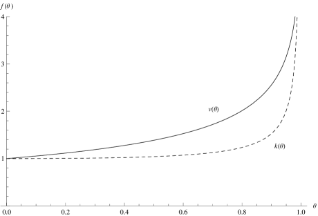
Figure 1: Multiplicative factors $v\left(\theta\right)$ (solid line) and $k\left(\theta\right)$ (dashed line).

Because of the values $v\left(\theta\right)$ can assume, $\text{Var}\left(\boldsymbol{X}\right)$ is an inflated version of $\boldsymbol{\Sigma}$, without limits about the degree of inflation that tends to $\infty$ when $\theta\rightarrow 1$. However, if $\theta\rightarrow 0$, then $v\left(\theta\right)\rightarrow 1$; so, under this case, $\text{Var}\left(\boldsymbol{X}\right)$ tends to $\boldsymbol{\Sigma}$.

According to (18), $\text{Kurt}\left(\boldsymbol{X}\right)$ is proportional to the kurtosis $d\left(d+2\right)$ of the (nested) MN distribution, with proportionality factor $k\left(\theta\right)$ depending on $\theta$. In particular, the function $k\left(\theta\right):\left(0,1\right)\rightarrow\left(1,\infty\right)$, given in (18) and graphically represented by a dashed line in Figure 1, is increasing in $\theta$. Therefore, $\text{Kurt}\left(\boldsymbol{X}\right)$ is greater than $d\left(d+2\right)$ meaning that the MTIN distribution allows for leptokurtosis. An upper bound for $\text{Kurt}\left(\boldsymbol{X}\right)$ does not exist since $k\left(\theta\right)\rightarrow\infty$ when $\theta\rightarrow 1$. However, if $\theta\rightarrow 0$, then $k\left(\theta\right)\rightarrow 1$; so, under this case, $\text{Kurt}\left(\boldsymbol{X}\right)$ tends to $d\left(d+2\right)$. There is another aspect to be noted from Figure 1. While $v\left(\theta\right)$ is a smoothly increasing function of $\theta$, $k\left(\theta\right)$ is approximately flat on the left, increasing suddenly only when $\theta$ is close to 1. From a practical point of view, this means that we need an high $\theta$-value to have a relevant excess kurtosis.

3 Maximum likelihood estimation

Several estimators of the parameters $\boldsymbol{\Psi}=\left\{\boldsymbol{\mu},\boldsymbol{\Sigma},\theta\right\}$ of the MTIN distribution may be considered. Among them, the maximum likelihood (ML) estimator is the most attractive because of its asymptotic properties (see, e.g., Pfanzagl and Hamböker, 1994, p. 206). Naturally, other estimation methods can be used; Appendix C gives details about the method of moments (MM). Below we discuss two possible ways to obtain the ML estimates of $\boldsymbol{\Psi}$; for their comparison, see Section 6.1.

3.1 Direct approach

Given a random sample $\boldsymbol{x}_{1},\ldots,\boldsymbol{x}_{n}$ (observed data) from $\boldsymbol{X}\sim\mathcal{TIN}_{d}\left(\boldsymbol{\mu},\boldsymbol{\Sigma},\theta\right)$, the ML estimation method is based on the maximization of the (observed-data) log-likelihood function

$$l\left(\boldsymbol{\Psi}\right) = n\log\left(2\right)-\frac{nd}{2}\log\left(\pi\right)-\frac{n}{2}\log\left|\boldsymbol{\Sigma}\right|-n\log\left(\theta\right)-\left(\frac{d}{2}+1\right)\sum_{i=1}^{n}\log\left[\delta\left(\boldsymbol{x}_{i};\boldsymbol{\mu},\boldsymbol{\Sigma}\right)\right]$$ (19)

$$+\sum_{i=1}^{n}\log\left[\Gamma\left(\frac{d}{2}+1,(1-\theta)\frac{\delta\left(\boldsymbol{x}_{i};\boldsymbol{\mu},\boldsymbol{\Sigma}\right)}{2}\right)-\Gamma\left(\frac{d}{2}+1,\frac{\delta\left(\boldsymbol{x}_{i};\boldsymbol{\mu},\boldsymbol{\Sigma}\right)}{2}\right)\right],$$

which does not admit a closed form solution. Furthermore, maximizing (19) with respect to $\boldsymbol{\Psi}$ is a constrained problem due to $\boldsymbol{\Sigma}$ and $\theta$. To make the maximization problem unconstrained, we apply the following reparameterization for $\boldsymbol{\Sigma}$ and $\theta$. According to the Cholesky decomposition we write

$$\boldsymbol{\Sigma}=\boldsymbol{\Omega}^{\prime}\boldsymbol{\Omega},$$

where $\boldsymbol{\Omega}$ is an upper triangular matrix with real-valued entries. As concerns $\theta$ we write

$$\theta=\frac{\exp(\gamma)}{1+\exp(\gamma)},$$

where $\gamma\in\real$. According to the above parametrization, the log-likelihood function in (19) can be re-written as

$$l\left(\boldsymbol{\Psi}^{*}\right) = n\log\left(2\right)-\frac{nd}{2}\log\left(\pi\right)-\frac{n}{2}\log\left|\boldsymbol{\Omega}^{\prime}\boldsymbol{\Omega}\right|-n\left\{\gamma-\log\left[1+\exp(\gamma)\right]\right\}$$ (20)

$$-\left(\frac{d}{2}+1\right)\sum_{i=1}^{n}\log\left[\delta\left(\boldsymbol{x}_{i};\boldsymbol{\mu},\boldsymbol{\Omega}^{\prime}\boldsymbol{\Omega}\right)\right]$$

$$+\sum_{i=1}^{n}\log\left\{\Gamma\left[\frac{d}{2}+1,\frac{\delta\left(\boldsymbol{x}_{i};\boldsymbol{\mu},\boldsymbol{\Omega}^{\prime}\boldsymbol{\Omega}\right)}{2\left[1+\exp(\gamma)\right]}\right]-\Gamma\left[\frac{d}{2}+1,\frac{\delta\left(\boldsymbol{x}_{i};\boldsymbol{\mu},\boldsymbol{\Omega}^{\prime}\boldsymbol{\Omega}\right)}{2}\right]\right\},$$

where $\boldsymbol{\Psi}^{*}=\left\{\boldsymbol{\mu},\boldsymbol{\Omega},\gamma\right\}$. Details about the first order partial derivatives of $l\left(\boldsymbol{\Psi}^{*}\right)$ in (20), with respect to $\boldsymbol{\mu}$, $\boldsymbol{\Omega}$ and $\gamma$, are given in Appendix F. Operationally, we perform unconstrained maximization of $l\left(\boldsymbol{\Psi}^{*}\right)$ with respect to $\boldsymbol{\Psi}^{*}$ via the general-purpose optimizer optim() for R (R Core Team, 2018), included in the stats package. Different algorithms, such as the Nelder-Mead or BFGS, can be used for maximization. They can be passed to optim() via the argument method. Once the maximum is determined, the estimates for $\boldsymbol{\Sigma}$ and $\theta$ are simply obtained by back-transformations. For a comparison, in terms of parameter recovery and computational times, between Nelder-Mead and BFGS algorithms applied to the direct ML estimation of $\boldsymbol{\Psi}$, see Section 6.1.

3.2 ECME algorithm

To circumvent the complexity of the direct ML approach discussed in Section 3.1, we could consider the application of the expectation-maximization (EM) algorithm (Dempster et al., 1977), which is the classical approach to find ML estimates for distributions belonging to the MNSM family. However, for the MTIN, the M-step is not well-defined (for the motivations we give in Appendix D), and the EM algorithm fails to converge. This is not a serious problem because ML estimates of $\boldsymbol{\Psi}$ can be still found, much more efficiently, by using the expectation-conditional maximization either (ECME) algorithm (Liu and Rubin, 1994). The higher efficiency of the ECME algorithm, with respect to the EM algorithm, has been also discussed with reference to another member of the MNSM family, the M$t$ distribution (see Liu and Rubin, 1994, 1995 and McLachlan and Krishnan, 2007, Section 5.8).

The ECME algorithm is an extension of the expectation-conditional maximum (ECM) algorithm (Meng and Rubin, 1993) which, in turn, is an extension of the EM algorithm (see McLachlan and Krishnan, 2007, Chapter 5, for details). The ECM algorithm replaces the M-step of the EM algorithm by a number of computationally simpler conditional maximization (CM) steps. The ECME algorithm generalizes the ECM algorithm by conditionally maximizing on some or all of the CM-steps the incomplete-data log-likelihood. As for the EM and ECM algorithms, the ECME algorithm monotonically increases the likelihood and reliably converges to a stationary point of the likelihood function (see Meng and van Dyk, 1997 and McLachlan and Krishnan, 2007, Chapter 5). Moreover, Liu and Rubin (1994) found the ECME algorithm to be nearly always faster than both the EM and ECM algorithms in terms of number of iterations, and that it can be faster in total computer time by orders of magnitude (see also McLachlan and Krishnan, 2007, Chapter 5).

For the application of any variant of the EM algorithm, in the light of the hierarchical representation of the MTIN distribution given in (9), it is convenient to view the observed data as incomplete. The complete data are $\left(\boldsymbol{x}_{1}^{\prime},w_{1}\right)^{\prime},\ldots,\left(\boldsymbol{x}_{n}^{\prime},w_{n}\right)^{\prime}$, where the missing variables $w_{1},\ldots,w_{n}$ are defined so that

$$\boldsymbol{X}_{i}|W_{i}=w_{i}\sim\mathcal{N}_{d}\left(\boldsymbol{\mu},\boldsymbol{\Sigma}/w_{i}\right),$$ (21)

independently for $i=1,\ldots,n$, and

$$W_{1},\ldots,W_{n}\stackrel{{\scriptstyle\text{i.i.d.}}}{{\sim}}\mathcal{U}\left(1-\theta,1\right).$$ (22)

Because of this conditional structure, the complete-data likelihood function $L_{c}\left(\boldsymbol{\Psi}\right)$ can be factored into the product of the conditional densities of $\boldsymbol{X}_{i}$ given the $w_{i}$ and the marginal densities of $W_{i}$, i.e.

$$L_{c}\left(\boldsymbol{\Psi}\right) = \prod_{i=1}^{n}f_{\text{N}}\left(\boldsymbol{x}_{i};\boldsymbol{\mu},\boldsymbol{\Sigma}/w_{i}\right)h_{\text{U}}\left(w_{i};1-\theta,1\right)$$ (23)

$$= \prod_{i=1}^{n}(2\pi)^{-\frac{d}{2}}w_{i}^{\frac{d}{2}}\left|\boldsymbol{\Sigma}\right|^{-\frac{1}{2}}\exp\left[-\frac{w_{i}}{2}\delta\left(\boldsymbol{x}_{i};\boldsymbol{\mu},\boldsymbol{\Sigma}\right)\right]\frac{1}{\theta}\text{1I}_{\left(1-\theta,1\right)}\left(w_{i}\right).$$

Accordingly, the complete-data log-likelihood function can be written as

$$l_{c}\left(\boldsymbol{\Psi}\right)=\log\left[L_{c}\left(\boldsymbol{\Psi}\right)\right]=l_{1c}\left(\boldsymbol{\mu},\boldsymbol{\Sigma}\right)+l_{2c}\left(\theta\right),$$ (24)

where

$$l_{1c}\left(\boldsymbol{\mu},\boldsymbol{\Sigma}\right)=-\displaystyle\frac{nd}{2}\log(2\pi)-\frac{n}{2}\log\left|\boldsymbol{\Sigma}\right|+\frac{d}{2}\sum_{i=1}^{n}\log\left(w_{i}\right)-\frac{1}{2}\sum_{i=1}^{n}w_{i}\delta\left(\boldsymbol{x}_{i};\boldsymbol{\mu},\boldsymbol{\Sigma}\right),$$ (25)

and

$$l_{2c}\left(\theta\right)=-n\log\left(\theta\right)+\sum_{i=1}^{n}\log\left[\text{1I}_{\left(1-\theta,1\right)}\left(w_{i}\right)\right].$$ (26)

The ECME algorithm iterates between three steps, one E-step and two CM-steps, until convergence. The two CM-steps arise from the partition of $\boldsymbol{\Psi}$ as $\left\{\boldsymbol{\Psi}_{1},\Psi_{2}\right\}$, where $\boldsymbol{\Psi}_{1}=\left\{\boldsymbol{\mu},\boldsymbol{\Sigma}\right\}$ and $\Psi_{2}=\theta$. These steps, for the generic $\left(r+1\right)$th iteration of the algorithm, $r=1,2,\ldots$, are detailed below.

3.2.1 E-step

The E-step requires the calculation of

$$Q\left(\boldsymbol{\Psi}|\boldsymbol{\Psi}^{(r)}\right)=Q_{1}\left(\boldsymbol{\mu},\boldsymbol{\Sigma}|\boldsymbol{\Psi}^{(r)}\right)+Q_{2}\left(\theta|\boldsymbol{\Psi}^{(r)}\right),$$ (27)

the conditional expectation of $l_{c}\left(\boldsymbol{\Psi}\right)$ given the observed data $\boldsymbol{x}_{1},\ldots,\boldsymbol{x}_{n}$, using the current fit $\boldsymbol{\Psi}^{(r)}$ for $\boldsymbol{\Psi}$. In (27) the two terms on the right-hand side are ordered as the two terms on the right-hand side of (24). As well-explained in McNeil et al. (2005, p. 82), in order to compute $Q\left(\boldsymbol{\Psi}|\boldsymbol{\Psi}^{(r)}\right)$ we need to replace any function $m\left(W_{i}\right)$ of the latent mixing variables which arise in (25) and (26) by the quantities $E_{\boldsymbol{\Psi}^{(r)}}\left[m\left(W_{i}\right)|\boldsymbol{X}_{i}=\boldsymbol{x}_{i}\right]$, where the expectation, as it can be noted by the subscript, is taken using the current fit $\boldsymbol{\Psi}^{(r)}$ for $\boldsymbol{\Psi}$, $i=1,\ldots,n$. To calculate these expectations we can observe that the conditional pdf of $W_{i}|\boldsymbol{X}_{i}=\boldsymbol{x}_{i}$ satisfies $f\left(w_{i}|\boldsymbol{x}_{i};\boldsymbol{\Psi}\right)\propto f\left(w_{i},\boldsymbol{x}_{i};\boldsymbol{\Psi}\right)$, up to some constant of proportionality. In detail,

$$f\left(w_{i}|\boldsymbol{x}_{i};\boldsymbol{\Psi}\right) \propto f\left(w_{i},\boldsymbol{x}_{i};\boldsymbol{\Psi}\right)$$ (28)

$$\propto w_{i}^{\frac{d}{2}+1-1}\exp\left[-\frac{\delta\left(\boldsymbol{x}_{i};\boldsymbol{\mu},\boldsymbol{\Sigma}\right)}{2}w_{i}\right]\text{1I}_{\left(1-\theta,1\right)}\left(w_{i}\right)$$

$$\propto \frac{1}{\eta\left(\boldsymbol{x}_{i};\boldsymbol{\Psi}\right)}f_{\text{G}}\left(w_{i};\frac{d}{2}+1,\frac{\delta\left(\boldsymbol{x}_{i};\boldsymbol{\mu},\boldsymbol{\Sigma}\right)}{2}\right)\text{1I}_{\left(1-\theta,1\right)}\left(w_{i}\right),$$

where

$$f_{\text{G}}\left(w;\alpha,\beta\right)=\frac{\beta^{\alpha}}{\Gamma\left(\alpha\right)}w^{\alpha-1}\exp\left(-\beta w\right)$$

denotes the pdf of a gamma distribution with parameters $\alpha>0$ and $\beta>0$ and

$$\eta\left(\boldsymbol{x}_{i};\boldsymbol{\Psi}\right)=\frac{1}{\Gamma\left(\frac{d}{2}+1\right)}\left[\Gamma\left(\frac{d}{2}+1,(1-\theta)\frac{\delta\left(\boldsymbol{x}_{i};\boldsymbol{\mu},\boldsymbol{\Sigma}\right)}{2}\right)-\Gamma\left(\frac{d}{2}+1,\frac{\delta\left(\boldsymbol{x}_{i};\boldsymbol{\mu},\boldsymbol{\Sigma}\right)}{2}\right)\right].$$

This means that $W_{i}|\boldsymbol{X}_{i}=\boldsymbol{x}_{i}$ has a doubly-truncated gamma distribution (Coffey and Muller, 2000), on the interval $\left(1-\theta,1\right)$, with parameters $d/2+1$ and $\delta\left(\boldsymbol{x}_{i};\boldsymbol{\mu},\boldsymbol{\Sigma}\right)/2$, whose pdf is given in (28); in symbols

$$W_{i}|\boldsymbol{X}_{i}=\boldsymbol{x}_{i}\sim\mathcal{DTG}_{\left(1-\theta,1\right)}\left(\frac{d}{2}+1,\frac{\delta\left(\boldsymbol{x}_{i};\boldsymbol{\mu},\boldsymbol{\Sigma}\right)}{2}\right).$$ (29)

Now, the functions $m\left(W_{i}\right)$ arising in (25) and (26) are $m_{1}\left(w\right)=w$, $m_{2}\left(w\right)=\log\left(w\right)$ and $m_{3}\left(w\right)=\log\left[\text{1I}_{\left(1-\theta,1\right)}\left(w\right)\right]$. However, there is no need to compute the expectation of $m_{2}$ since the term $\log\left(W_{i}\right)$ is not related with the parameters; moreover, there is no need to compute the expectation of $m_{3}$ because we do not use $Q_{2}\left(\theta|\boldsymbol{\Psi}^{(r)}\right)$ to update $\theta$. Thanks to (29) we have that

$$E_{\boldsymbol{\Psi}^{(r)}}\left(W_{i}|\boldsymbol{X}_{i}=\boldsymbol{x}_{i}\right)=w_{i}^{(r)},$$ (30)

where

$$w_{i}^{(r)}= \frac{2\>\left[\Gamma\left(\frac{d}{2}+2,\left(1-\theta^{(r)}\right)\frac{\delta\left(\boldsymbol{x}_{i};\boldsymbol{\mu}^{(r)},\boldsymbol{\Sigma}^{(r)}\right)}{2}\right)-\Gamma\left(\frac{d}{2}+2,\frac{\delta\left(\boldsymbol{x}_{i};\boldsymbol{\mu}^{(r)},\boldsymbol{\Sigma}^{(r)}\right)}{2}\right)\right]}{\Gamma\left(\frac{d}{2}+1\right)\eta\left(\boldsymbol{x}_{i};\boldsymbol{\Psi}^{(r)}\right)\delta\left(\boldsymbol{x}_{i};\boldsymbol{\mu}^{(r)},\boldsymbol{\Sigma}^{(r)}\right)}$$

$$= \frac{2}{\delta\left(\boldsymbol{x}_{i};\boldsymbol{\mu}^{(r)},\boldsymbol{\Sigma}^{(r)}\right)}\frac{\left[\Gamma\left(\frac{d}{2}+2,\left(1-\theta^{(r)}\right)\frac{\delta\left(\boldsymbol{x}_{i};\boldsymbol{\mu}^{(r)},\boldsymbol{\Sigma}^{(r)}\right)}{2}\right)-\Gamma\left(\frac{d}{2}+2,\frac{\delta\left(\boldsymbol{x}_{i};\boldsymbol{\mu}^{(r)},\boldsymbol{\Sigma}^{(r)}\right)}{2}\right)\right]}{\left[\Gamma\left(\frac{d}{2}+1,\left(1-\theta^{(r)}\right)\frac{\delta\left(\boldsymbol{x}_{i};\boldsymbol{\mu}^{(r)},\boldsymbol{\Sigma}^{(r)}\right)}{2}\right)-\Gamma\left(\frac{d}{2}+1,\frac{\delta\left(\boldsymbol{x}_{i};\boldsymbol{\mu}^{(r)},\boldsymbol{\Sigma}^{(r)}\right)}{2}\right)\right]}.$$ (31)

Then, by substituting $w_{i}$ with $w_{i}^{(r)}$ in the last term on the right-hand side of (25), we obtain

$$Q_{1}\left(\boldsymbol{\mu},\boldsymbol{\Sigma}|\boldsymbol{\Psi}^{(r)}\right)=-\frac{n}{2}\log\left|\boldsymbol{\Sigma}\right|-\frac{1}{2}\sum_{i=1}^{n}w_{i}^{(r)}\delta\left(\boldsymbol{x}_{i};\boldsymbol{\mu},\boldsymbol{\Sigma}\right),$$

where the terms constant with respect to $\boldsymbol{\mu}$ and $\boldsymbol{\Sigma}$ are dropped.

3.2.2 CM-step 1

The first CM-step, at the same iteration, requires the calculation of $\boldsymbol{\Psi}_{1}^{\left(r+1\right)}$ as the value of $\boldsymbol{\Psi}_{1}$ that maximizes $Q_{1}\left(\boldsymbol{\mu},\boldsymbol{\Sigma}|\boldsymbol{\Psi}^{(r)}\right)$, with respect to $\boldsymbol{\mu}$ and $\boldsymbol{\Sigma}$, with $\Psi_{2}$ fixed at $\Psi_{2}^{(r)}$. Theis maximization is easily implemented if we note that $Q_{1}$ is a weighted log-likelihood, with weights $w_{1}^{(r)},\ldots,w_{n}^{(r)}$, of $n$ independent observations $\boldsymbol{x}_{1},\ldots,\boldsymbol{x}_{n}$ from $\mathcal{N}_{d}\left(\boldsymbol{\mu},\boldsymbol{\Sigma}/w_{1}^{(r)}\right),\ldots,\mathcal{N}_{d}\left(\boldsymbol{\mu},\boldsymbol{\Sigma}/w_{n}^{(r)}\right)$, respectively. So, the updates for $\boldsymbol{\mu}$ and $\boldsymbol{\Sigma}$ are

$$\boldsymbol{\mu}^{(r+1)}=\displaystyle\frac{1}{\displaystyle\sum_{i=1}^{n}w_{i}^{(r)}}\sum_{i=1}^{n}w_{i}^{(r)}\boldsymbol{x}_{i}$$ (32)

and

$$\boldsymbol{\Sigma}^{(r+1)}=\frac{1}{n}\sum_{i=1}^{n}w_{i}^{(r)}\left(\boldsymbol{x}_{i}-\boldsymbol{\mu}^{\left(r+1\right)}\right)\left(\boldsymbol{x}_{i}-\boldsymbol{\mu}^{\left(r+1\right)}\right)^{\prime}.$$ (33)

3.2.3 CM-step 2

In the second CM-step, at the same iteration, $\Psi_{2}=\theta$ is chosen to maximize the observed-data log-likelihood function $l\left(\boldsymbol{\Psi}\right)$, as given by (19), with $\boldsymbol{\Psi}_{1}$ fixed at $\boldsymbol{\Psi}_{1}^{(r+1)}$. In detail, from (19) we have

$$l\left(\left\{\boldsymbol{\Psi}_{1}^{(r+1)},\theta\right\}\right)= n\log\left(2\right)-\frac{nd}{2}\log\left(\pi\right)-\frac{n}{2}\log\left|\boldsymbol{\Sigma}^{(r+1)}\right|-n\log\left(\theta\right)-\left(\frac{d}{2}+1\right)\sum_{i=1}^{n}\log\left[\delta\left(\boldsymbol{x}_{i};\boldsymbol{\mu}^{(r+1)},\boldsymbol{\Sigma}^{(r+1)}\right)\right]$$

$$+\sum_{i=1}^{n}\log\left[\Gamma\left(\frac{d}{2}+1,(1-\theta)\frac{\delta\left(\boldsymbol{x}_{i};\boldsymbol{\mu}^{(r+1)},\boldsymbol{\Sigma}^{(r+1)}\right)}{2}\right)-\Gamma\left(\frac{d}{2}+1,\frac{\delta\left(\boldsymbol{x}_{i};\boldsymbol{\mu}^{(r+1)},\boldsymbol{\Sigma}^{(r+1)}\right)}{2}\right)\right].$$ (34)

Thus, the second CM-step of the ECME algorithm chooses $\theta^{(r+1)}$ to maximize (34) with $\boldsymbol{\mu}=\boldsymbol{\mu}^{(r+1)}$ and $\boldsymbol{\Sigma}=\boldsymbol{\Sigma}^{(r+1)}$. This implies that $\theta^{(r+1)}$ is a solution of the equation

$$-\frac{n}{\theta}+\left(1-\theta\right)^{\frac{d}{2}}\sum_{i=1}^{n}\frac{\left[\frac{\delta\left(\boldsymbol{x}_{i};\boldsymbol{\mu}^{(r+1)},\boldsymbol{\Sigma}^{(r+1)}\right)}{2}\right]^{\frac{d}{2}+1}\exp\left[-\frac{\left(1-\theta\right)\delta\left(\boldsymbol{x}_{i};\boldsymbol{\mu}^{(r+1)},\boldsymbol{\Sigma}^{(r+1)}\right)}{2}\right]}{\Gamma\left(\frac{d}{2}+1,(1-\theta)\frac{\delta\left(\boldsymbol{x}_{i};\boldsymbol{\mu}^{(r+1)},\boldsymbol{\Sigma}^{(r+1)}\right)}{2}\right)-\Gamma\left(\frac{d}{2}+1,\frac{\delta\left(\boldsymbol{x}_{i};\boldsymbol{\mu}^{(r+1)},\boldsymbol{\Sigma}^{(r+1)}\right)}{2}\right)}=0.$$ (35)

As a closed form solution for the root of (35) is not analytically available, we use the uniroot() function in the stats package of R to perform the numerical one-dimensional search of $\theta\in(0,1)$.

4 Existence of the ML estimates

In this section we demonstrate the existence of the ML estimates for $\boldsymbol{\mu}$, $\boldsymbol{\Sigma}$, and $\theta$. With this aim, we consider the solutions from the ECME algorithm of Section 3.2. In line with the CM-steps of the algorithm, we first demonstrate the existence of $\boldsymbol{\mu}$ and $\boldsymbol{\Sigma}$, given $\theta$ (Theorem 4.1), and then the existence of $\theta$ given $\boldsymbol{\mu}$ and $\boldsymbol{\Sigma}$ (Theorem 4.2).

Theorem 4.1.

Given $\theta$ and a sample $\boldsymbol{x}_{1},\ldots,\boldsymbol{x}_{n}$, if $n>d\left(\frac{d}{2}+1\right)$, then there exists $(\widehat{\boldsymbol{\mu}},\widehat{\boldsymbol{\Sigma}})\in{}^{d}\times\mathcal{M}^{+}_{d\times d}$, being $\mathcal{M}^{+}_{d\times d}$ the set of positive-definite symmetric $d\times d$ matrices, such that

$$l\left(\widehat{\boldsymbol{\mu}},\widehat{\boldsymbol{\Sigma}},\theta\right)\geq l\left(\boldsymbol{\mu},\boldsymbol{\Sigma},\theta\right),\quad\text{for every}\ (\boldsymbol{\mu},\boldsymbol{\Sigma})\in{}^{d}\times\mathcal{M}^{+}_{d\times d}.$$ (36)

Proof.

The pdf of $\boldsymbol{X}\sim\mathcal{TIN}_{d}\left(\boldsymbol{\mu},\boldsymbol{\Sigma},\theta\right)$ can be written as

$$f_{\text{TIN}}\left(\boldsymbol{x};\boldsymbol{\mu},\boldsymbol{\Sigma},\theta\right)=\left|\boldsymbol{\Sigma}\right|^{-\frac{1}{2}}g\left[\delta\left(\boldsymbol{x};\boldsymbol{\mu},\boldsymbol{\Sigma}\right)\right],$$

where

$$g(t)=\frac{2\pi^{-\frac{d}{2}}}{\theta t^{\left(\frac{d}{2}+1\right)}}\left[\Gamma\left(\frac{d}{2}+1,(1-\theta)\frac{t}{2}\right)-\Gamma\left(\frac{d}{2}+1,\frac{t}{2}\right)\right].$$

To prove the theorem we use Proposition 2.4 in Cuesta-Albertos et al. (2008). In particular, it is sufficient to verify that the following assumptions are valid:

1. there exists a strictly decreasing sequence $\left\{t_{n}\right\}$ which converges to zero, such that $g(t_{n})<g(t_{n+1})$ for every $n$;

2. if $d>1$, then there exists $\gamma>d/2$ such that $\displaystyle\lim_{r\rightarrow\infty}r^{\gamma}g(r)=0$;

3. $g(\cdot)$ is continuous on ⁺.

While (G3) is easily verifiable, (G1) and (G2) need some attention. To verify (G1) we can consider the first derivative of $g(\cdot)$, i.e.

$$g^{\prime}(t)=-\frac{2\pi^{-\frac{d}{2}}}{\theta t^{\left(\frac{d}{2}+2\right)}}\left[\Gamma\left(\frac{d}{2}+2,(1-\theta)\frac{t}{2}\right)-\Gamma\left(\frac{d}{2}+2,\frac{t}{2}\right)\right].$$

It is straightforward to verify that $g^{\prime}(t)<0$ for all $t\in{}^{+}$; so, (G1) is satisfied for any strictly decreasing sequence $\left\{t_{n}\right\}$ which converges to zero.

In order to verify (G2), consider $\gamma=\frac{d}{2}+1>\frac{d}{2}$. Then

$$r^{\frac{d}{2}+1}g(r) = \frac{2\pi^{-\frac{d}{2}}}{\theta}\left[\Gamma\left(\frac{d}{2}+1,(1-\theta)\frac{t}{2}\right)-\Gamma\left(\frac{d}{2}+1,\frac{t}{2}\right)\right]$$ (37)

$$= \frac{2\pi^{-\frac{d}{2}}}{\theta}\left(\int_{0}^{\frac{r}{2}}\exp(-x)x^{\frac{d}{2}+1}dx-\int^{(1-\theta)\frac{r}{2}}_{0}\exp(-x)x^{\frac{d}{2}+1}dx\right).$$

When $r\rightarrow\infty$, both the integrals in (37) tend to $\Gamma\left(\frac{d}{2}+2\right)$, so that $\lim_{r\rightarrow\infty}r^{\gamma}g(r)=0$. Then, (G2) is verified for $\gamma=\frac{d}{2}+1$. ∎

Theorem 4.2.

Given $\boldsymbol{\mu}$, $\boldsymbol{\Sigma}$, and a sample $\boldsymbol{x}_{1},\ldots,\boldsymbol{x}_{n}$, then there exists $\widehat{\theta}\in\left(0,1\right)$ such that

$$l\left(\boldsymbol{\mu},\boldsymbol{\Sigma},\widehat{\theta}\right)\geq l\left(\boldsymbol{\mu},\boldsymbol{\Sigma},\theta\right),\quad\text{for every $\theta\in\left(0,1\right)$}.$$ (38)

Proof.

According to (7), and given $\boldsymbol{\mu}$ and $\boldsymbol{\Sigma}$, the log-likelihood function results

$$l\left(\boldsymbol{\mu},\boldsymbol{\Sigma},\theta\right)=l\left(\theta\right)=-\frac{nd}{2}\log\left(2\pi\right)-\frac{n}{2}\log\left|\boldsymbol{\Sigma}\right|+\sum_{i=1}^{n}\log\left\{\frac{1}{\theta}\int_{1-\theta}^{1}w^{\frac{d}{2}}\exp\left[-\frac{w}{2}{\delta\left(\boldsymbol{x}_{i};\boldsymbol{\mu},\boldsymbol{\Sigma}\right)}\right]dw\right\}.$$ (39)

It is straightforward to realize that $l\left(\theta\right)$ is continuous in $(0,1)$. If the limits of $l\left(\theta\right)$, when $\theta$ tends to the boundaries $0$ and $1$ of the support, are both finite, then the log-likelihood function has a maximum and the theorem is proved. When $\theta\rightarrow 1$ we have

$$\lim_{\theta\rightarrow 1}l\left(\theta\right)=-\frac{nd}{2}\log\left(2\pi\right)-\frac{n}{2}\log\left|\boldsymbol{\Sigma}\right|+\sum_{i=1}^{n}\log\left\{\int_{0}^{1}w^{\frac{d}{2}}\exp\left[-\frac{w}{2}{\delta\left(\boldsymbol{x}_{i};\boldsymbol{\mu},\boldsymbol{\Sigma}\right)}\right]dw\right\}.$$

When $\theta\rightarrow 0$, using the results in (3)–(4), we obtain

$$\lim_{\theta\rightarrow 0}l\left(\theta\right)=-\frac{nd}{2}\log\left(2\pi\right)-\frac{n}{2}\log\left|\boldsymbol{\Sigma}\right|-\frac{1}{2}\sum_{i=1}^{n}\delta\left(\boldsymbol{x}_{i};\boldsymbol{\mu},\boldsymbol{\Sigma}\right).$$ (40)

The limit in (40) is constant and corresponds to the log-likelihood function of a $d$-variate normal distribution computed in $\boldsymbol{\mu}$ and $\boldsymbol{\Sigma}$. ∎

5 Some notes on robustness

The MTIN model allows to obtain improved (in terms of robustness) ML estimates of $\boldsymbol{\mu}$ and $\boldsymbol{\Sigma}$, with respect to those provided by the nested (reference) MN model, in the presence of mild outliers. In detail, the influence of the observations $\boldsymbol{x}_{i}$ is reduced (down-weighted) as the squared Mahalanobis distance $\delta\left(\boldsymbol{x}_{i};\boldsymbol{\mu},\boldsymbol{\Sigma}\right)=\delta_{i}$ increases. This is in line with the $M$-estimation (Maronna, 1976) which uses a decreasing weighting function $w\left(\delta_{i}\right):\left(0,\infty\right)\rightarrow\left(0,\infty\right)$ to down-weight the observations $\boldsymbol{x}_{i}$ with large $\delta_{i}$ values. To be more precise, according to (32) and (33), $\boldsymbol{\mu}^{(r+1)}$ and $\boldsymbol{\Sigma}^{(r+1)}$ can be respectively viewed, since $\theta$ is estimated from the data by ML, as an adaptively weighted sample mean and sample covariance matrix, in the sense used by Hogg (1974), with weights $w_{i}^{(r)}$ given in (31). This approach, in addition to be a type of $M$-estimation, follows Box (1980) and Box and Tiao (2011) in embedding the reference MN model in a larger model with one or more parameters (here $\theta$) that afford protection against non-normality.

For each possible value of the dimension $d$, consider the weights $w_{i}^{(r)}$ in (31) as a bivariate (weighting) function $w$ of the squared Mahalanobis distance $\delta\geq 0$ and of the inflation parameter $\theta\in\left(0,1\right)$, i.e.

$$w\left(\delta,\theta;d\right)=\frac{2\left[\Gamma\left(\frac{d}{2}+2,\left(1-\theta\right)\frac{\delta}{2}\right)-\Gamma\left(\frac{d}{2}+2,\frac{\delta}{2}\right)\right]}{\delta\left[\Gamma\left(\frac{d}{2}+1,\left(1-\theta\right)\frac{\delta}{2}\right)-\Gamma\left(\frac{d}{2}+1,\frac{\delta}{2}\right)\right]}.$$ (41)

It is straightforward to show that the weighting function in (41) is positive. An example of graphical representation of $w\left(\delta,\theta;d\right)$, in the case $d=3$, is provided in Figure 2.

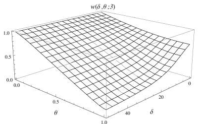
Figure 2: Graphical representation of $w\left(\delta,\theta;d=3\right)$.

As concerns the limiting behavior of $w\left(\delta,\theta;d\right)$ as $\delta\rightarrow\infty$, by using the fundamental theorem of calculus and l’H$\hat{\mbox{o}}$spital’s rule we obtain

$$\lim_{\delta\rightarrow\infty}w\left(\delta,\theta;d\right)=1-\theta.$$ (42)

From (42) we note that, when observations are very far from the bulk of the data ($\delta\rightarrow\infty$) their weight in the computation of $\boldsymbol{\mu}$ and $\boldsymbol{\Sigma}$ depends by $\theta$. If $\theta$ is close to zero (i.e. if the MTIN approaches the MN distribution), then the weight is close to one; indeed, this is what we expect under the normal case. In the other cases, the weight linearly decreases as $\theta$ increases, i.e. as the MTIN departs from the MN distribution. As concerns the limiting behavior of $w\left(\delta,\theta;d\right)$ as $\theta\rightarrow 0$, by using the mathematics considered for the limit in (42), we have

$$\lim_{\theta\rightarrow 0}w\left(\delta,\theta;d\right)=1.$$ (43)

From (43) we can observe that if $\theta\rightarrow 0$, then $w\left(\delta,\theta;d\right)\rightarrow 1$ regardless of $\delta$, and this happens because we are operationally working with a MN distribution (see Theorem 2.1).

6 Simulation studies

In this section, we investigate various aspects related to our model through simulation studies. While the simulation study of Section 6.1 is considered to evaluate parameter recovery of the proposed estimation procedures, in addition to the computational times required by these procedures, the simulation study of Section 6.2 aims to compare classical model selection criteria in selecting among a set of well-established elliptical distributions, with differing number of parameters, including the MTIN. The whole analysis is conducted in R and the code for density evaluation, random number generation, and fitting for the MTIN distribution is available, in the form of an R package named mtin, from http://docenti.unict.it/punzo/Rpackages.htm.

6.1 Parameter recovery and computational times

In this section we compare two methods to estimate the parameters of the MTIN distribution, namely the method of moments (MM), discussed in Appendix C, and ML, discussed in Section 3. These methods are compared with respect to parameter recovery and to the computational time required. We use three approaches to compute ML estimates: direct approach with the Nelder-Mead algorithm, direct approach with the BFGS algorithm, and ECME algorithm (cf. Section 3). All the algorithms used to obtain ML estimates are initialized by the solution provided by the method of moments.

In this study we consider three experimental factors: the dimension ($d\in\left\{2,3,5\right\}$), the sample size ($n\in\left\{200,500,1000\right\}$), and the inflation parameter ($\theta\in\left\{0.6,0.7,0.8,0.9\right\}$). The values of $\theta$ are chosen unbalanced on the right simply to have scenarios with more excess kurtosis (refer to the considerations made at the end of Section 2.3).

For each combination of $n$, $d$ and $\theta$, we sample one hundred datasets from a MTIN distribution with a zero mean vector ($\boldsymbol{\mu}=\boldsymbol{0}$) and an identity scale matrix ($\boldsymbol{\Sigma}=\boldsymbol{I}$), for a total of $3\times 3\times 4\times 100=3600$ datasets. On each generated dataset, we fit the MTIN distribution with the four approaches cited above. Computation is performed on a Windows 10 PC, with Intel i7-8550U CPU, 16.0 GB RAM, using R 64-bit, and the elapsed time (in seconds) is computed via the system.time() function of the base package. Parallel computing, using 4 cores, is considered.

We start evaluating parameter recovery by focusing on $\theta$; we limit the investigation to this parameter because, in analogy with other normal scale mixtures, the parameter(s) governing the tail-weight is (are) the most difficult to be estimated. However, although not reported here, the ranking of the estimation methods we obtain with respect to $\theta$ are roughly preserved when we move to $\boldsymbol{\mu}$ and $\boldsymbol{\Sigma}$.

In Figure 3 we report the box-plots of the differences $(\hat{\theta}-\theta)$, for bias evaluation, while in Figure 4 we report the box-plots of the squared differences $(\hat{\theta}-\theta)^{2}$, for mean square error (MSE) evaluation. Each of the nine plots in these figures refers to a particular pair $\left(n,d\right)$ and shows $4\times 3=12$ box-plots each summarizing (for every $\theta$ and used method) the behavior of the considered differences with respect to the available 100 replications. As expected, the differences under evaluation improve as $n$ increases. Interestingly enough, the differences improves when either $d$ or $\theta$ increase. Regardless of the scenario and difference considered, BFGS and ECME algorithms for ML estimation work comparably and represent the best approaches. The worst approach is MM. The very similar behavior between BFGS and ECME algorithms can be further corroborated by looking at Table 1, where log-likelihood values are averaged over the 100 replications of each triplet $\left(n,d,\theta\right)$. Here we can note how these algorithms return exactly the same average results, which are always slightly better than those provided by the Nelder-Mead algorithm, and this is true regardless of the triplet $\left(n,d,\theta\right)$ considered. To be more precise, looking at the whole set of obtained results (not reported here for the sake of space), BFGS and ECME algorithms provide, on each fitted model, the same maximized log-likelihood value.

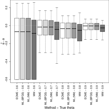
(a) $d=2$ and $n=200$

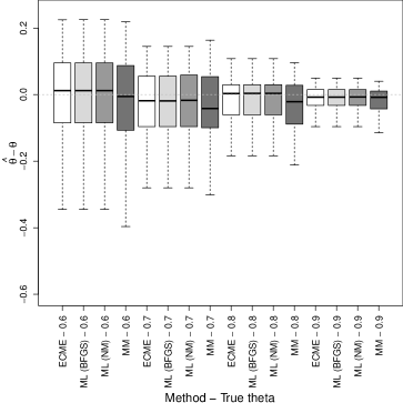
(b) $d=2$ and $n=500$

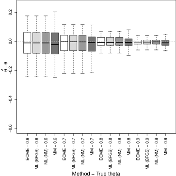
(c) $d=2$ and $n=1000$

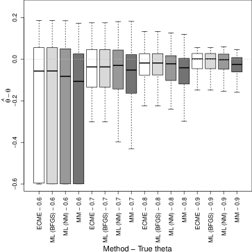
(d) $d=3$ and $n=200$

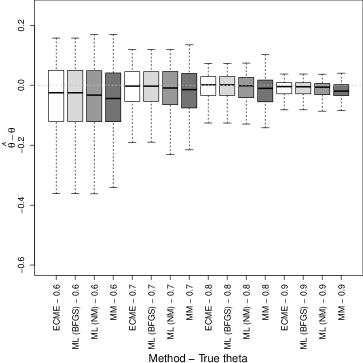
(e) $d=3$ and $n=500$

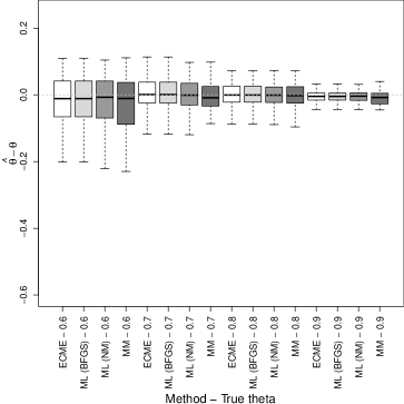
(f) $d=3$ and $n=1000$

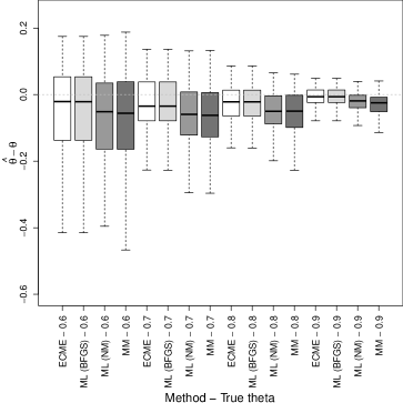
(g) $d=5$ and $n=200$

(h) $d=5$ and $n=500$

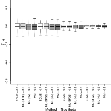
(i) $d=5$ and $n=1000$

Figure 3: Box-plots of the differences $(\hat{\theta}-\theta)$ for each pair $\left(n,d\right)$. The box-plot in each subfigure summarize the results over 100 replications and refers to a combination between $\theta$ and the estimation method considered.

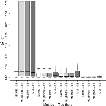
(a) $d=2$ and $n=200$

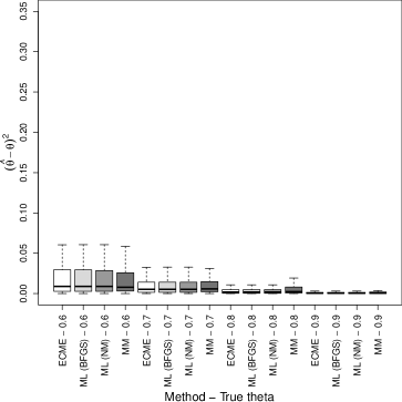
(b) $d=2$ and $n=500$

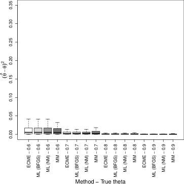
(c) $d=2$ and $n=1000$

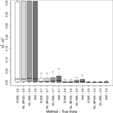
(d) $d=3$ and $n=200$

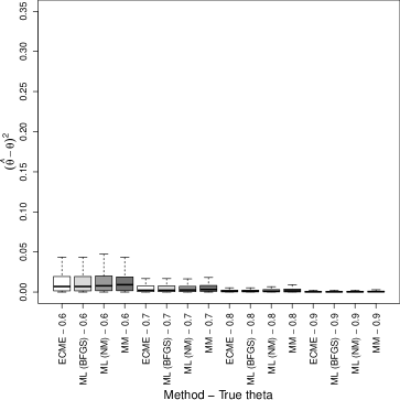
(e) $d=3$ and $n=500$

(f) $d=3$ and $n=1000$

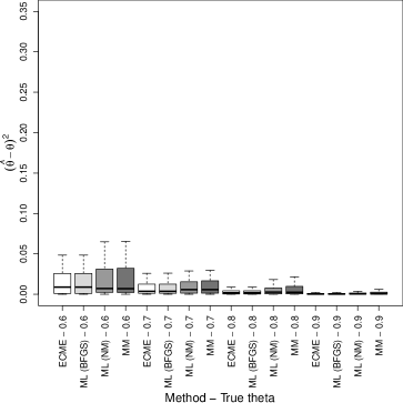
(g) $d=5$ and $n=200$

(h) $d=5$ and $n=500$

(i) $d=5$ and $n=1000$

Figure 4: Box-plots of the differences $(\hat{\theta}-\theta)^{2}$ for each pair $\left(n,d\right)$. The box-plot in each subfigure summarize the results over 100 replications and refers to a combination between $\theta$ and the estimation method considered.

Table 1: Log-likelihoods values averaged over 100 replications.

			ML direct
$n$	$d$	$\theta$	Nelder-Mead	BFGS	ECME
200	2	0.6	-649.860	-649.860	-649.860
		0.7	-674.456	-674.456	-674.456
		0.8	-699.929	-699.928	-699.928
		0.9	-744.023	-744.023	-744.023
	3	0.6	-973.686	-973.680	-973.680
		0.7	-1009.362	-1009.341	-1009.341
		0.8	-1051.155	-1051.113	-1051.113
		0.9	-1107.200	-1107.120	-1107.120
	5	0.6	-1620.323	-1620.245	-1620.245
		0.7	-1677.022	-1676.873	-1676.873
		0.8	-1744.074	-1743.715	-1743.715
		0.9	-1844.226	-1843.270	-1843.270
500	2	0.6	-1623.352	-1623.353	-1623.353
		0.7	-1686.506	-1686.505	-1686.505
		0.8	-1758.846	-1758.846	-1758.846
		0.9	-1853.362	-1853.369	-1853.369
	3	0.6	-2433.665	-2433.656	-2433.656
		0.7	-2532.655	-2532.629	-2532.629
		0.8	-2639.989	-2639.930	-2639.930
		0.9	-2785.396	-2785.292	-2785.292
	5	0.6	-4066.467	-4066.397	-4066.397
		0.7	-4209.660	-4209.510	-4209.510
		0.8	-4376.644	-4376.347	-4376.347
		0.9	-4613.231	-4612.413	-4612.413
1000	2	0.6	-3257.490	-3257.490	-3257.490
		0.7	-3368.835	-3368.835	-3368.835
		0.8	-3513.907	-3513.906	-3513.906
		0.9	-3722.987	-3722.986	-3722.986
	3	0.6	-4887.646	-4887.634	-4887.634
		0.7	-5050.221	-5050.197	-5050.197
		0.8	-5270.342	-5270.311	-5270.311
		0.9	-5558.195	-5558.122	-5558.122
	5	0.6	-8125.940	-8125.868	-8125.868
		0.7	-8418.000	-8417.825	-8417.825
		0.8	-8759.827	-8759.525	-8759.525
		0.9	-9241.587	-9240.833	-9240.833

As concerns the computational times, for each combination of $\theta$ and the estimation method considered, Figure 5 reports the box-plots of the elapsed times in each of the $3\times 3\times 100=900$ replications obtained marginalizing with respect to $n$ and $d$.

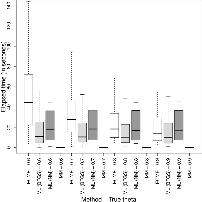
Figure 5: Elapsed time (in seconds) on each combination between $\theta$ and the estimation method considered. Each box plot refers to $3\times 3\times 100=900$ values obtained summing out with respect to $d\in\left\{2,3,5\right\}$ and $n\in\left\{200,500,1000\right\}$.

The MM provides the best (lowest) elapsed times, regardless of the true underlying $\theta$. Among the algorithms considered to obtain ML estimates, the BFGS is the best one, followed by the Nelder-Mead and ECME algorithms. The elapsed times from the ECME algorithm seem to be a decreasing function of $\theta$, tying those of the BFGS algorithm when $\theta=0.9$. Another interesting result can be noted by looking at Figure 6 where we report, analogously to Figure 5, the box plots of the elapsed times only in the case $d=5$, when varying the sample size.

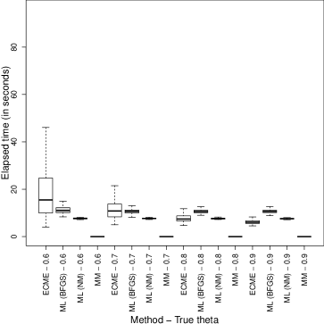
(a) $d=5$ and $n=200$

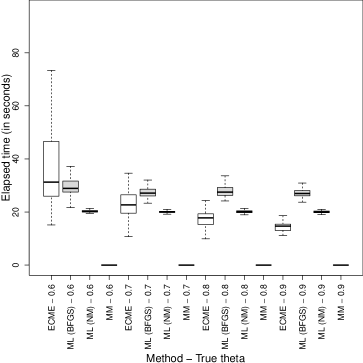
(b) $d=5$ and $n=500$

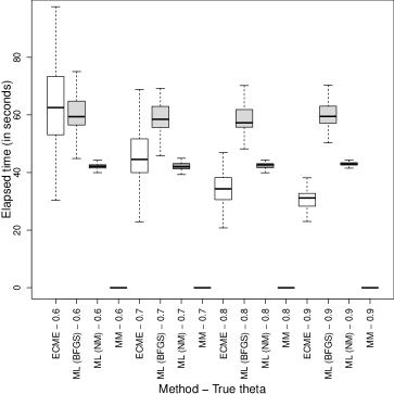
(c) $d=5$ and $n=1000$

Figure 6: Elapsed time (in seconds) in the case $d=5$ on each combination between $\theta$ and the estimation method considered, when varying $n\in\left\{200,500,1000\right\}$. Each box plot refers to 100 replications.

Indeed, the ECME algorithm provides the best elapsed times for high values of $\theta$ (say $\theta>0.7$), regardless of the sample size. Other simulations with greater values of $d$, not reported here for the sake of space, have shown that the ECME is the fastest algorithm to obtain ML estimates, and this is true regardless of $\theta$.

Summarizing, giving prominence to parameter recovery, we suggest to use the ML approach. Among the three algorithms considered to obtain ML estimates, we suggest direct ML via the BFGS algorithm for low dimensions (say $d<4$) and the ECME algorithm for high dimensions (say $d>10$). In the other cases, the choice also depends on the value of the true but unknown inflation parameter. A possible solution may be to preliminary run the method of moments and, if the MM-estimated value of $\theta$ is high, then using the ECME algorithm, and using the BFGS algorithm otherwise.

6.2 Model selection: AIC versus BIC

Model selection is usually required to select among a set of candidate models with differing number of parameters. The classical way to perform this selection is via the computation of a convenient (likelihood-based) model selection criterion. Two widely considered choices, that in our formulation need to be maximized, are the Akaike information criterion (AIC; Akaike, 1974)

$$\text{AIC}=2l\left(\widehat{\boldsymbol{\Psi}}\right)-2\times\#\text{par},$$

and the Bayesian information criterion (BIC; Schwarz, 1978)

$$\text{BIC}=2l\left(\widehat{\boldsymbol{\Psi}}\right)-\ln n\times\#\text{par},$$

where $\#\text{par}$ is the overall number of free parameters in the model. AIC and BIC are similar, but with a different penalty for the number of parameters. BIC penalizes free parameters more strongly than AIC if $n>7$. For both, the models being compared need not to be nested, unlike the case when models are being compared using, for example, a likelihood ratio test (Greselin and Punzo, 2013 and Punzo et al., 2016). A comparison of AIC and BIC is given by Burnham and Anderson (2013, Section 6.3–6.4), with follow-up remarks by Burnham and Anderson (2004). BIC is argued to be appropriate for selecting the “true model” (i.e. the process that generated the data) from the set of candidate models. To be specific, if the “true model” is in the set of candidates, then BIC will select it with probability 1, as $n\rightarrow\infty$; in contrast, when selection is done via AIC, the probability can be less than 1 (Burnham and Anderson, 2013, Section 6.3–6.4, Vrieze, 2012, and Aho et al., 2014). Proponents of AIC argue that this issue is negligible, because the “true model” is virtually never in the candidate set. If the “true model” is not in the candidate set, then the most that we can hope to do is select the model that best approximates the “true model”. AIC is appropriate for finding the best approximating model, under certain assumptions.

In this section we compare the performance of AIC and BIC. We consider two experimental factors: the dimension ($d\in\left\{2,3\right\}$) and the data generating process (DGP). The sample size is instead fixed to $n=1000$. As DGPs, in addition to the MN and MTIN, we consider several multivariate elliptical heavy-tailed distributions used in the literature. They are the M$t$, MLN, MCN, MSVG, MSH, SNIG, and MSGH distributions given in Section 2.2, with the MLN denoting the multivariate leptokurtic normal distribution introduced by Bagnato et al. (2017). All the DGPs share a zero mean vector ($\boldsymbol{\mu}=\boldsymbol{0}$) and an identity scale matrix ($\boldsymbol{\Sigma}=\boldsymbol{I}$). The remaining parameter(s) governing the tail-weight of the heavy-tailed competing distributions are: $\nu=4.5$ (degrees of freedom) for the M$t$, $\theta=0.99$ (inflation parameter) for the MTIN, $\beta=6$ (excess kurtosis) for the MLN, $\alpha=0.9$ and $\eta=5$ (proportion of good points and degree of contamination) for the MCN, $\lambda=\psi=3$ for the MSVG, $\chi=0.5$ and $\psi=3$ for the MSH, $\chi=3$ and $\psi=0.2$ for the SNIG, and $\lambda=\chi=\psi=0.1$ for the MSGH; for details about the parameters $\lambda$, $\chi$ and $\psi$ of the distributions within the MSGH family, refer to Appendix E.

For each combination of the simulation factors, one-hundred replications are considered, yielding a total of $9\times 2\times 100=1800$ generated datasets. For each, we fit all the models in the considered set of DGPs. Parameters are estimated based on the ML approach. We adopt the ECME algorithm for the MTIN distribution. As concerns the competing models, we use the WML.MLN() function of the code available at http://www.olddei.unict.it/punzo/Rcode.htm to fit the MLN, the CNmixt() function of the ContaminatedMixt package (Punzo et al., 2018a, b) to fit the MCN, and the ghyp package (Luethi and Breymann, 2016) to fit the remaining models.

Tables 2 and 3 show the percentage of times AIC and BIC select each model in the cases $d=2$ and $d=3$, respectively. Results are organized as a contingency table where the true DGP is given by column and the fitted models by row. Each cell of the contingency table reports two selection counts referred to AIC (on the top) and BIC (on the bottom). The cells on the diagonal reports a sort of true positive percentage (TPP), measuring the percentage of times that each criterion is able to discover the true DGP. We can note how, regardless of $d$, the criteria are able enough to recognize the true underlying DGP being the counts mainly concentrated on the diagonal cells; however, for some DGPs within the MSGH family, such as the MSVG and MSH, their considerable similarity makes discovering the true model more difficult. This is probably due to the considered parameterizations under the MSVG and MSH DGPs. The last column of each table shows the average number of times a model different from the underlying DGP is selected; this can be meant as a sort of false positive percentage (FPP). The ideal situation for AIC and BIC should have zero off-diagonal values.

		True
Fitted		MN	Mt	MTIN	MLN	MCN	MSVG	MSH	SNIG	MSGH	FPP
MN	AIC	91	0	0	0	0	0	0	0	0	0.000
	BIC	100	0	0	0	0	0	0	0	0	0.000
Mt	AIC	1	68	11	0	8	3	4	5	0	4.000
	BIC	0	68	11	0	20	3	4	5	0	5.375
MTIN	AIC	1	16	88	0	1	7	8	2	0	4.375
	BIC	0	16	88	0	12	7	10	2	0	5.875
MLN	AIC	6	0	0	100	0	12	0	0	0	2.250
	BIC	0	0	0	100	0	14	0	0	0	1.750
MCN	AIC	0	0	0	0	91	6	7	1	0	1.750
	BIC	0	0	0	0	68	0	0	0	0	0.000
MSVG	AIC	1	0	0	0	0	56	18	3	0	2.750
	BIC	0	0	0	0	0	56	18	4	1	2.875
MSH	AIC	0	1	0	0	0	10	33	0	0	1.375
	BIC	0	1	0	0	0	14	37	0	0	1.875
SNIG	AIC	0	15	0	0	0	6	30	84	0	6.375
	BIC	0	15	0	0	0	6	31	89	0	6.500
MSGH	AIC	0	0	1	0	0	0	0	5	100	0.750
	BIC	0	0	1	0	0	0	0	0	99	0.125

Table 2: Percentage of times AIC and BIC select each model. The true DGP is shown by column, while the fitted models are given by row. The last column provides the false positive percentage (FPP).

		True
Fitted		MN	M$t$	MTIN	MLN	MCN	MSVG	MSH	SNIG	MSGH	FPP
MN	AIC	96	0	0	0	0	0	0	0	0	0.000
	BIC	100	0	0	0	0	0	0	0	0	0.000
M$t$	AIC	0	77	5	0	1	1	0	0	1	1.000
	BIC	0	78	5	0	6	1	0	4	6	2.750
MTIN	AIC	1	8	94	0	1	3	0	1	1	1.875
	BIC	0	8	95	0	1	3	0	1	1	1.750
MLN	AIC	3	0	0	97	0	2	0	0	0	0.625
	BIC	0	0	0	100	0	4	0	0	0	0.500
MCN	AIC	0	0	1	3	98	7	1	0	0	1.500
	BIC	0	0	0	0	93	1	0	0	0	0.125
MSVG	AIC	0	0	0	0	0	56	23	1	0	3.000
	BIC	0	0	0	0	0	56	24	1	0	3.125
MSH	AIC	0	0	0	0	0	22	41	0	0	2.750
	BIC	0	0	0	0	0	26	42	0	0	3.250
SNIG	AIC	0	13	0	0	0	9	31	83	0	6.625
	BIC	0	14	0	0	0	9	34	93	0	0.000
MSGH	AIC	0	2	0	0	0	0	4	15	98	2.625
	BIC	0	0	0	0	0	0	0	1	93	0.125

Table 3: Percentage of times AIC and BIC select each model. The true DGP is shown by column, while the fitted models are given by row. The last column provides the false positive percentage (FPP).

The first aspect we note is that, as expected, the AIC tends to select less parsimonious models. As an example, consider Table 2. On the one hand, under a MN-DGP, the BIC always discovers the true model, while the AIC selects 8 times models with an additional parameter (M$t$, MTIN, and MLN), and one time a model with two additional parameters (MSGV). On the other hand, under a MCN-DGP, the truth is discovered 91 times by the AIC and only 68 times by the BIC. This happens because the BIC has a propensity for more parsimonious models such as the M$t$ and MTIN, having only one additional parameter with respect to the MN. Regardless of the considered number of dimensions, another aspect we note is that, for some DGPs within the MSGH family, such as the MSVG and MSH, their considerable similarity makes assessment of the true model challenging. In summary, it is difficult to establish the best model selection criterion among those considered; thus, we will use both in the real data analyses presented in Section 7.

7 Financial applications

Risk management and portfolio selection are interesting financial areas of application of the proposed MTIN distribution. In these areas, one of the main problems is the modelling of the joint distribution of stock-prices and asset-returns. So, the models that are commonly considered are inherently multivariate, as stressed by McNeil et al. (2005, Chapter 3), with the MN distribution playing a special rule (Kring et al., 2008 and Rachev et al., 2010, Chapter 14). However, many empirical studies show that the MN is not appropriate for the distribution of risk factor returns and stock returns (see, e.g., Mandelbrot, 1963 and Fama, 1965). Two possible motivations for this inappropriateness concern its elliptical symmetry and thin tails (Bingham et al., 2002). While the former assumption is not a limitation, as shown by McNeil et al. (2005, Section 3.3) via empirical studies, the latter one is more harmful since the MN-tails are not consistent with the empirical heavy tails of the distribution of returns. This has motivated numerous proposals for alternative parametric multivariate elliptical heavy-tailed distributions. One of the most famous proposals in this direction is represented by the multivariate $\alpha$-stable sub-Gaussian (M$\alpha$SSG) distributions (see, e.g., Kring et al., 2008). Unfortunately, these distributions are so heavy-tailed that the second moment is infinite, a fact that is inconsistent with empirical findings for most financial returns (Bingham et al., 2002) and with the fact that many theoretical models in finance rely on the existence of this moment (Rachev et al., 2010, p. 290). A further drawback of the M$\alpha$SSG distributions is that, with a few exceptions, they do not possess an analytic expression for the pdf (Kring et al., 2008, p. 112). This is the reason why other multivariate elliptical heavy-tailed distributions, such as those from the MNSM family (see Section 2.2.1), are typically preferred for financial modelling.

Motivated by the above considerations, the proposed MTIN model is compared, on real financial data, with the same multivariate elliptical heavy-tailed distributions already considered in Section 6.2, which are also widely used in the financial literature. Parameters are estimated based on the ML approach, under the common simplifying assumption that returns form iid samples (see, e.g., McNeil et al., 2005, p. 84). Computational details have been already discussed in Section 6. The comparison is made in terms of AIC, BIC, and appropriateness of the fitted models in reproducing the empirical kurtosis.

We fit the competing models to three multivariate time series related to 4 of the 30 large publicly owned companies considered by the Dow Jones index. The companies are American Express (AXP), Boeing (BA), Intel (INTC), and Microsoft (MSFT). All the codes needed to replicate the analysis are included in the Supplementary Material. We consider daily log-returns spanning the period from January 5th, 2015 to December 1th, 2017 ($n=734$ observations downloadable from http://finance.yahoo.com/). The matrix of scatter plots is displayed in Figure 7.

Figure 7: Pairwise scatter plots of daily log-returns of the quadruple $(\textsf{AXP},\textsf{BA},\textsf{INTC},\textsf{MSFT})$ spanning the period from January 5th, 2015 to December 1th, 2017.

Table 4 provides some descriptive statistics (and Jarque-Bera normality tests) for the AXP, BA, INTC, and MSFT series, separately considered.

Table 4: Descriptive statistics, and Jarque-Bera normality tests (with $p$-values in brackets), for the AXP, BA, INTC, and MSFT series.

		Mean	Std. Dev	Excess kurtosis	Jarque-Bera test
AXP		0.000	0.013	17.648	9756.065 ($<$ 0.001)
BA		0.001	0.014	8.116	2022.966 ($<$ 0.001)
INTC		0.000	0.014	5.574	970.972 ($<$ 0.001)
MSFT		0.000	0.014	10.964	3508.548 ($<$ 0.001)

All the series are leptokurtic and the Jarque-Bera statistic confirms the departure from univariate normality at the 1${}^{\text{o}}\mkern-5.0mu/\mkern-3.0mu_{\text{oo}}$ level. As concerns the dependence between stocks, Table 5 displays the pairwise sample correlations along with $p$-values from the tests of uncorrelation computed via the cor.test() function of the stats package.

Table 5: Pairwise correlations between AXP, BA, INTC, and MSFT. $p$-values from the tests of pairwise uncorrelation are given in brackets.

	BA	INTC	MSFT
AXP	0.342	0.311	0.294
	($<$ 0.001)	($<$ 0.001)	($<$ 0.001)
BA		0.400	0.362
		($<$ 0.001)	($<$ 0.001)
INTC			0.569
			($<$ 0.001)

As we can see, the four correlations are all significantly different from zero confirming the need of a multivariate model allowing for correlation between series.

7.1 Bivariate example

In the first example we consider the bivariate ($d=2$) time series of log-returns of AXP and BA stocks. Table 6 presents a comparison of the models in terms of goodness-of-fit and ability in reproducing the empirical kurtosis, which is 43.04. Table 6 also gives rankings induced by AIC, BIC, and by the absolute difference between estimated and empirical kurtosis. The estimated kurtosis is computed analytically, by substituting the estimated parameters in the theoretical formula for the kurtosis. The theoretical kurtosis is given in (16) for the MTIN, in Appendix E for the MSGH models (along with their particular subcases), in Kotz and Nadarajah (2004) for the M$t$, and in Bagnato et al. (2017) for MLN and MCN models.

Model	$\#$ par.	Log-lik.	AIC	Ranking	BIC	Ranking	Kurtosis	Abs. diff.	Ranking
MN	5	4306.900	8603.800	9	8580.808	9	8	35.043	7
M$t$	6	4559.031	9106.063	2	9078.472	2	-	-	9
MTIN	6	4561.830	9111.661	1	9084.070	1	44.539	1.497	1
MLN	6	4453.772	8895.545	8	8867.953	8	14.400	28.643	4
MCN	7	4549.373	9084.747	4	9052.557	5	27.929	15.114	2
MSVG	7	4521.768	9031.536	6	9003.945	6	14.083	28.960	5
MSH	7	4521.450	9030.901	7	9003.310	7	13.065	29.977	6
SNIG	7	4547.695	9083.390	5	9055.798	4	20.241	22.801	3
MSGH	8	4559.031	9104.062	3	9071.873	3	82.140	39.097	8

Table 6: Bivariate example: log-likelihood, AIC, BIC and kurtosis for the competing models, along with rankings induced by these criteria. The column “Abs. diff.” denotes the absolute difference between empirical and estimated kurtoses. The empirical kurtosis is 43.04.

As we can see from Table 6, AIC and BIC provide the same ranking, except for the SNIG and MCN distributions having a reversed position. These criteria indicate that the MTIN is the best model; its estimated inflation parameter is $\widehat{\theta}=0.993$ (very close to the upper bound for this parameter). The second and third best models are the M$t$ and MSGH, respectively. For the M$t$ model, the estimated degrees of freedom are lower than $4$ ($\widehat{\nu}=3.371$) and, as such, the corresponding kurtosis is undefined. Among the competing models, the MTIN is the best one also in reproducing the empirical kurtosis (the absolute difference is 1.497). According to this criterion, the second best model is the MCN; interestingly, although the MCN model has an additional parameter with respect to the MTIN, it provides a worse result.

7.2 Trivariate example

In the second example we consider the trivariate ($d=3$) time series of log-returns of the AXP, BA, and INTC stocks. AIC and BIC in Table 7 provide, for the fitted models, the same ranking. As for the previous example, considering AIC and BIC, the MTIN, M$t$, and MSGH models occupy the first, second, and third positions, respectively. The estimated inflation parameter ($\widehat{\theta}=0.990$) is close to the upper bound also in this case.

The estimated degrees of freedom for the M$t$ distribution are lower than $4$ also in this example ($\widehat{\nu}=3.497$); then, we can not evaluate the ability of the M$t$ model in reproducing the empirical kurtosis (63.48). According to the absolute difference between estimated and empirical kurtosis, the best model is the MTIN while the second best is the MCN.

Model	$\#$ par.	Log-Lik.	AIC	Ranking	BIC	Ranking	Kurtosis	Abs. diff.	Ranking
MN	9	6499.588	12981.180	9	12939.790	9	15	48.488	8
M$t$	10	6843.439	13666.880	2	13620.890	2	-	-	9
MTIN	10	6843.689	13667.380	1	13621.390	1	68.182	4.693	1
MLN	10	6631.859	13243.720	8	13197.730	8	27.000	36.488	5
MCN	11	6820.018	13618.040	5	13567.450	5	45.330	18.158	2
MSVG	11	6802.071	13584.140	6	13538.160	6	25.872	37.616	6
MSH	11	6792.339	13564.680	7	13518.690	7	22.500	40.988	7
SNIG	11	6831.064	13642.130	4	13596.140	4	35.843	27.646	3
MSGH	12	6843.438	13664.880	3	13614.290	3	94.084	30.596	4

Table 7: Trivariate example: log-likelihood, AIC, BIC and kurtosis for the competing models, along with rankings induced by these criteria. The column “Abs. diff.” denotes the absolute difference between empirical and estimated kurtoses. The empirical kurtosis is 63.48.

7.3 Quadrivariate example

In the third example we consider the quadrivariate ($d=4$) time series of log-returns of the AXP, BA, INTC, and MSFT stocks. According to AIC and BIC, which provide the same ranking (see Table 8), the MTIN, M$t$, and MSGH models occupy the first, second, and third positions, respectively. The estimated inflation parameter results $\widehat{\theta}=0.990$, while the estimated degrees of freedom are $\widehat{\nu}=3.453$. As concerns the kurtosis, the model having the best performance is the MTIN while the second best, as in the previous two examples, is the MCN.

Model	$\#$ par.	Log-Lik.	AIC	Ranking	BIC	Ranking	Kurtosis	Abs. diff.	Ranking
MN	14	8740.774	17453.550	9	17389.170	9	24	74.474	7
M$t$	15	9236.442	18442.880	2	18373.910	2	-	-	9
MTIN	15	9236.793	18443.590	1	18374.610	1	109.293	10.819	1
MLN	15	8934.125	17838.250	8	17769.270	8	40.000	58.475	5
MCN	16	9198.779	18365.560	5	18291.980	5	70.307	28.168	2
MSVG	16	9180.549	18331.100	6	18262.120	6	41.269	57.206	4
MSH	16	9150.832	18271.660	7	18202.690	7	33.600	64.874	6
SNIG	16	9220.903	18411.810	4	18342.830	4	57.865	40.609	3
MSGH	17	9236.443	18440.890	3	18367.310	3	182.387	83.912	8

Table 8: Quadrivariate example: log-likelihood, AIC, BIC and kurtosis for the competing models, along with rankings induced by these criteria. The column “Abs. diff.” denotes the absolute difference between empirical and estimated kurtoses. The empirical kurtosis is 98.474.

8 Discussion

In this article, the multivariate tail-inflated normal (MTIN) distribution has been introduced. Compared with other multivariate heavy-tailed elliptical distributions embedding the multivariate normal (MN), the MTIN has the following main characteristics:

• a closed-form representation for the probability density function (differently from the $\alpha$-stable sub-Gaussian distributions, with the exception of the Cauchy distribution);

• a single parameter governing the tail weight (differently from the contaminated normal distribution and from the majority of distributions nested within the symmetric generalized hyperbolic);

• an MN scale mixture representation (differently from the leptokurtic normal distribution);

• the covariance matrix and excess kurtosis always exist (differently from $t$ and $\alpha$-stable sub-Gaussian distributions);

• any level of excess kurtosis can be reached (differently from the leptokurtic normal distribution).

Moreover, being a member of the MN scale mixture family, the MTIN distribution allows to obtain robust estimates of the parameters of the nested MN distribution when the maximum likelihood estimation paradigm is considered, as discussed in Section 5. The analysis on financial data of Section 7 has further corroborated how the proposed model represents a valid alternative to most of the distributions cited above in terms of AIC and BIC, but also in reproducing the empirical kurtosis of the analyzed data that, in the considered financial context, is typically very high.

Appendix

Appendix A Alternative formulations of the pdf

An analogous formulation of the pdf in (1) is

$$f_{\text{TIN}}\left(\boldsymbol{x};\boldsymbol{\mu},\boldsymbol{\Sigma},\theta\right)=\frac{2\pi^{-\frac{d}{2}}\left|\boldsymbol{\Sigma}\right|^{-\frac{1}{2}}}{\theta\left[\delta\left(\boldsymbol{x};\boldsymbol{\mu},\boldsymbol{\Sigma}\right)\right]^{\left(\frac{d}{2}+1\right)}}\left[\gamma\left(\frac{d}{2}+1,\frac{\delta\left(\boldsymbol{x};\boldsymbol{\mu},\boldsymbol{\Sigma}\right)}{2}\right)-\gamma\left(\frac{d}{2}+1,(1-\theta)\frac{\delta\left(\boldsymbol{x};\boldsymbol{\mu},\boldsymbol{\Sigma}\right)}{2}\right)\right],$$ (A.1)

where $\gamma\left(\cdot,\cdot\right)$ is the lower incomplete gamma function. A further formulation of the pdf in (1) is

$$f_{\text{TIN}}\left(\boldsymbol{x};\boldsymbol{\mu},\boldsymbol{\Sigma},\theta\right)= \frac{2\pi^{-\frac{d}{2}}\left|\boldsymbol{\Sigma}\right|^{-\frac{1}{2}}}{\theta\left[\delta\left(\boldsymbol{x};\boldsymbol{\mu},\boldsymbol{\Sigma}\right)\right]^{\left(\frac{d}{2}+1\right)}}\left\{\sum_{i=0}^{\left\lfloor\frac{d}{2}\right\rfloor}\left(\frac{d}{2}\right)_{i}\left(\frac{\delta\left(\boldsymbol{x};\boldsymbol{\mu},\boldsymbol{\Sigma}\right)}{2}\right)^{\frac{d}{2}-i}\left[\exp\left(\frac{(1-\theta)\delta\left(\boldsymbol{x};\boldsymbol{\mu},\boldsymbol{\Sigma}\right)}{2}\right)\left(1-\theta\right)^{\frac{d}{2}-1}-1\right]\right.$$

$$\left.+\sqrt{\pi}\left(\frac{d}{2}\right)_{\frac{d-1}{2}}\left[\Phi\left(\sqrt{\delta\left(\boldsymbol{x};\boldsymbol{\mu},\boldsymbol{\Sigma}\right)}\right)-\Phi\left(\sqrt{(1-\theta)\delta\left(\boldsymbol{x};\boldsymbol{\mu},\boldsymbol{\Sigma}\right)}\right)\right]\text{1I}_{\left\{\frac{1}{2}\right\}}\left(\frac{d}{2}-\left\lfloor\frac{d}{2}\right\rfloor\right)\right\},$$ (A.2)

where $\left\lfloor\cdot\right\rfloor$ is the floor function, $(a)_{b}$ is the Pochhammer operator (Abramowitz and Stegun, 1965), and $\Phi(\cdot)$ is the distribution function of a standard normal random variable. The alternative form in (A.2) can be easily obtained by iteratively using the integration by parts to solve the integral in (7). Note that this formulation of the MTIN distribution simplifies if $d$ is even because the second row in (A.2) vanishes.

Appendix B Proof of Theorem 2.4

Before to sketch the proof of Theorem 2.4, we recall Definition B.1, which is discussed in more details in McNeil et al. (2005, Section 3.2.2), and we provide Theorem B.1 along its proof. These preparatory results give us the possibility to demonstrate Theorem 2.4.

Definition B.1 (MNSM: elliptical representation).

A random vector $\boldsymbol{X}$ is said to have a multivariate normal scale mixture (MNSM) distribution if

$$\boldsymbol{X}=\boldsymbol{\mu}+\sqrt{V}T\boldsymbol{\Lambda}\boldsymbol{U},$$ (B.1)

where $\boldsymbol{\mu}$, $T$, $\boldsymbol{\Lambda}$, and $\boldsymbol{U}$ are defined as in (10), while $V$ is a non-negative random variable which is independent of $T$ and $\boldsymbol{U}$.

Theorem B.1 (MNSM: mean vector, covariance matrix and kurtosis).

If $\boldsymbol{X}$ has a MNSM distribution, then

$$\mbox{E}\left(\boldsymbol{X}\right) = \boldsymbol{\mu},$$ (B.2)

$$\text{Var}\left(\boldsymbol{X}\right) = E(V)\boldsymbol{\Sigma},$$ (B.3)

$$\mbox{Kurt}\left(\boldsymbol{X}\right) = d\left(d+2\right)\frac{E\left(V^{2}\right)}{\left[E\left(V\right)\right]^{2}}.$$ (B.4)

Proof.

Results in (B.2) and (B.3) are proved in McNeil et al. (2005, p. 74). The result in (B.4) follows by

$$\mbox{Kurt}(\boldsymbol{X}) = \mbox{E}\left\{\left[\left(\boldsymbol{X}-\boldsymbol{\mu}\right)^{\prime}\left[\mbox{Var}\left(\boldsymbol{X}\right)\right]^{-1}\left(\boldsymbol{X}-\boldsymbol{\mu}\right)\right]^{2}\right\}$$

$$= \mbox{E}\left\{\left[\left(\boldsymbol{X}-\boldsymbol{\mu}\right)^{\prime}\left[\mbox{E}(V)\boldsymbol{\Sigma}\right]^{-1}\left(\boldsymbol{X}-\boldsymbol{\mu}\right)\right]^{2}\right\}$$

$$= \frac{1}{\left[\mbox{E}(V)\right]^{2}}\mbox{E}\left[\left(T^{2}V\boldsymbol{U}^{\prime}\boldsymbol{\Lambda}^{\prime}\boldsymbol{\Sigma}^{-1}\boldsymbol{\Lambda}\boldsymbol{U}\right)^{2}\right]$$

$$= \mbox{E}\left(T^{4}\right)\frac{\mbox{E}\left(V^{2}\right)}{\left[\mbox{E}(V)\right]^{2}}$$

$$= d(d+2)\frac{\mbox{E}\left(V^{2}\right)}{\left[\mbox{E}(V)\right]^{2}}.$$

∎

We are now ready to give the proof of Theorem 2.4.

Proof of Theorem 2.4.

The MTIN distribution, having the stochastic representation in (10), is a particular MNSM where $V$ has the inverse uniform distribution over the interval $\left(1,1/\left(1-\theta\right)\right)$. In such a case,

$$\mbox{E}(V)=-\frac{\log(1-\theta)}{\theta}\quad\mbox{and}\quad\mbox{E}\left(V^{2}\right)=\frac{1}{1-\theta}.$$ (B.5)

The result in (14) is verified by (B.2). The results in (15) and (16) are obtained by substituting the moments given in (B.5) in (B.3) and (B.4), respectively. ∎

Appendix C Method of moments

In the method of moments applied to the estimation of the parameters of the MTIN distribution, we relate the (unknown) population moments in (14), (15), and (16) to their sample counterparts

$$\overline{\boldsymbol{x}}=\frac{1}{n}\sum_{i=1}^{n}\boldsymbol{x}_{i},\quad\boldsymbol{S}=\frac{1}{n-1}\sum_{i=1}^{n}\left(\boldsymbol{x}_{i}-\overline{\boldsymbol{x}}\right)\left(\boldsymbol{x}_{i}-\overline{\boldsymbol{x}}\right)^{\prime},\quad\text{and}\quad\widehat{\text{Kurt}}(\boldsymbol{X})=\frac{1}{n}\sum_{i=1}^{n}\left[\left(\boldsymbol{x}_{i}-\overline{\boldsymbol{x}}\right)^{\prime}\boldsymbol{S}^{-1}\left(\boldsymbol{x}_{i}-\overline{\boldsymbol{x}}\right)\right]^{2}.$$

Solving the system of equations

$$\begin{cases}\boldsymbol{\mu}=\overline{\boldsymbol{x}}\\ v\left(\theta\right)\boldsymbol{\Sigma}=\boldsymbol{S}\\ k\left(\theta\right)d\left(d+2\right)=\max\left\{\widehat{\text{Kurt}}(\boldsymbol{X}),d\left(d+2\right)\right\}\end{cases}$$

with respect to $\boldsymbol{\mu}$, $\boldsymbol{\Sigma}$, and $\theta$, gives raise to the estimates $\widehat{\boldsymbol{\mu}}=\overline{\boldsymbol{x}}$ and $\widehat{\boldsymbol{\Sigma}}=\boldsymbol{S}/v(\widehat{\theta})$ for $\boldsymbol{\mu}$ and $\boldsymbol{\Sigma}$, respectively, where $\widehat{\theta}$ is determined by numerically solving the third equation of the system with respect to $\theta$. To search for this root in the interval $\left(0,1\right)$, we can use the uniroot() function included in the stats package. Finally note that, the third equation in the system involves the maximum because the MTIN distribution can not be platykurtic.

Appendix D Problems with the application of the EM algorithm

In the EM algorithm applied to the ML estimation of $\boldsymbol{\Psi}$ for the MTIN distribution, $\boldsymbol{\Psi}$ is taken as a whole. On the $(r+1)$th iteration of the EM algorithm, the E-step is the same as given in Section (3.2.1) for the ECME algorithm; instead, the two CM-steps are replaced by a single M-step which maximizes $Q\left(\boldsymbol{\Psi}|\boldsymbol{\Psi}^{(r)}\right)$ in (27). As the two terms of $Q\left(\boldsymbol{\Psi}|\boldsymbol{\Psi}^{(r)}\right)$, namely $Q_{1}\left(\boldsymbol{\mu},\boldsymbol{\Sigma}|\boldsymbol{\Psi}^{(r)}\right)$ and $Q_{2}\left(\theta|\boldsymbol{\Psi}^{(r)}\right)$, have zero-cross derivatives, they can be maximized separately with respect to the parameters they involve. Maximizing $Q_{1}\left(\boldsymbol{\mu},\boldsymbol{\Sigma}|\boldsymbol{\Psi}^{(r)}\right)$ with respect to $\boldsymbol{\mu}$ and $\boldsymbol{\Sigma}$ corresponds to the first CM-step of the ECME algorithm (cf. Section 3.2.2). As it can be noted from (26), maximizing $Q_{2}\left(\theta|\boldsymbol{\Psi}^{(r)}\right)$ with respect to $\theta$ is equivalent to maximize the log-likelihood function of $n$ independent observations $w_{1}^{(r)},\ldots,w_{n}^{(r)}$ from $\mathcal{U}\left(1-\theta,1\right)$. Hence, we do not need to compute $\text{E}_{\boldsymbol{\Psi}^{(r)}}\left\{\log\left[\text{1I}_{\left(1-\theta,1\right)}\left(W_{i}|\boldsymbol{X}_{i}=\boldsymbol{x}_{i}\right)\right]\right\}$ in the E-step. Therefore, from the standard theory about the uniform distribution (see, e.g., Johnson and Kotz, 1970, Chapter 26), the update for $\theta$ is

$$\theta^{(r+1)}=1-w_{(1)}^{(r)},$$ (D.1)

where $w_{(1)}^{(r)}=\min\left(w_{1}^{(r)},\ldots,w_{n}^{(r)}\right)$. Unfortunately, according to (30), it happens that $\theta^{(r+1)}<\theta^{(r)}$ because $w_{(1)}^{(r)}\in\left(1-\theta^{(r)},1\right)$. This means that $\theta^{(r)}$ is a decreasing function of $r$, and this yields

$$\lim_{r\rightarrow\infty}\theta^{(r)}=0,$$

regardless of the true but unknown value of $\theta$. So, the EM algorithm fails to converge.

Appendix E Kurtosis of the symmetric generalized hyperbolic distribution

As well-documented in McNeil et al. (2005, Section 3.2), the MSGH distribution belongs to the MNSM family if $V$ in (B.1) has a generalized inverse Gaussian distribution; in symbols, $V\sim\mathcal{N}^{-}\left(\lambda,\chi,\psi\right)$. In particular, if $\boldsymbol{X}$ has a MSGH distribution, in symbols $\boldsymbol{X}\sim\mathcal{SGH}_{d}\left(\boldsymbol{\mu},\boldsymbol{\Sigma},\lambda,\chi,\psi\right)$, then its pdf is

$$f_{\text{MSGH}}\left(\boldsymbol{x};\boldsymbol{\mu},\boldsymbol{\Sigma},\lambda,\chi,\psi\right)=\frac{\left(\sqrt{\chi\psi}\right)^{-\lambda}\psi^{\frac{d}{2}}}{\left(2\pi\right)^{\frac{d}{2}}\left|\boldsymbol{\Sigma}\right|^{\frac{1}{2}}K_{\lambda}\left(\sqrt{\chi\psi}\right)}\frac{K_{\lambda-\frac{d}{2}}\left(\sqrt{\left[\chi+\delta\left(\boldsymbol{x};\boldsymbol{\mu},\boldsymbol{\Sigma}\right)\right]\psi}\right)}{\left\{\sqrt{\left[\chi+\delta\left(\boldsymbol{x};\boldsymbol{\mu},\boldsymbol{\Sigma}\right)\right]\psi}\right\}^{\frac{d}{2}-\lambda}},$$ (E.1)

where $K_{\lambda}(\cdot)$ is the modified Bessel function of the third kind with index $\lambda$ (see Abramowitz and Stegun, 1965, for details). The parameters $\lambda$, $\chi$, and $\psi$ satisfy the following conditions: if $\lambda<0$, then $\chi>0$ and $\psi\geq 0$; if $\lambda=0$, then $\chi>0$ and $\psi>0$; if $\lambda>0$, then $\chi\geq 0$ and $\psi\geq 0$.

In the following we provide the kurtosis for the MSGH distribution (Theorem E.1) as well as for the nested SNIG, MSH (Corollary E.1), and MSVG (Corollary E.2) distributions.

Theorem E.1 (MSGH: kurtosis).

If $\boldsymbol{X}\sim\mathcal{SGH}_{d}\left(\boldsymbol{\mu},\boldsymbol{\Sigma},\lambda,\chi,\psi\right)$, then

$$\mbox{Kurt}\left(\boldsymbol{X}\right)=d\left(d+2\right)\frac{K_{\lambda+2}\left(\sqrt{\chi\psi}\right)K_{\lambda}\left(\sqrt{\chi\psi}\right)}{K_{\lambda+1}\left(\sqrt{\chi\psi}\right)^{2}}.$$ (E.2)

Proof.

If $\boldsymbol{X}\sim\mathcal{SGH}_{d}\left(\boldsymbol{\mu},\boldsymbol{\Sigma},\lambda,\chi,\psi\right)$, then it can be expressed as in (B.1) with $V\sim\mathcal{N}^{-}(\lambda,\chi,\psi)$. For the non-limiting case $\chi>0$ and $\psi>0$, it results (see McNeil et al., 2005, Section A.2.5)

$$\mbox{E}\left(V^{\alpha}\right)=\left(\frac{\chi}{\psi}\right)^{\frac{\alpha}{2}}\frac{K_{\lambda+\alpha}\left(\sqrt{\chi\psi}\right)}{K_{\lambda+\alpha}\left(\sqrt{\chi\psi}\right)}.\quad\alpha\in\real.$$ (E.3)

Then, setting $\alpha=1$ and $\alpha=2$ in (E.3), the first and second moments of $V$ are respectively obtained. Once $\mbox{E}\left(V\right)$ and $\mbox{E}\left(V^{2}\right)$ are substituted in (B.4), (E.2) is obtained. ∎

Corollary E.1 (SNIG and MSH: kurtosis).

The kurtosis of the SNIG and MSH distributions are

$$\mbox{Kurt}\left(\boldsymbol{X}\right)=d\left(d+2\right)\frac{K_{\frac{3}{2}}\left(\sqrt{\chi\psi}\right)K_{-\frac{1}{2}}\left(\sqrt{\chi\psi}\right)}{K_{\frac{1}{2}}\left(\sqrt{\chi\psi}\right)^{2}}$$ (E.4)

and

$$\mbox{Kurt}\left(\boldsymbol{X}\right)=d\left(d+2\right)\frac{K_{3}\left(\sqrt{\chi\psi}\right)K_{1}\left(\sqrt{\chi\psi}\right)}{K_{2}\left(\sqrt{\chi\psi}\right)^{2}},$$ (E.5)

respectively.

Proof.

If $\lambda=-0.5$ and $\lambda=1$ are substituted in (E.2), then the results in (E.4) and (E.5) are obtained, respectively. ∎

As concerns the kurtosis of the MSVG distribution, we have a particular simplification of (E.2) which is detailed in the following corollary.

Corollary E.2 (MSVG: kurtosis).

If $\lambda>0$ and $\chi=0$ in Theorem E.1, leading (E.1) to be the pdf of the MSVG distribution, then

$$\mbox{Kurt}\left(\boldsymbol{X}\right)=d\left(d+2\right)\frac{\lambda+1}{\lambda}.$$ (E.6)

Proof.

If $\lambda>0$ and $\chi=0$, then the random variable $V$ has a gamma distribution with parameters $\alpha=\lambda$ and $\beta=\frac{1}{2}\psi$. In this case, the MSGH distribution in (E.1) reduces to the MSVG distribution. Then, by substituting the first two moments

$$\mbox{E}(V)=\frac{2\lambda}{\psi}\quad\mbox{and}\quad\mbox{E}\left(V^{2}\right)=\frac{4\lambda(\lambda+1)}{\psi^{2}}$$

in (B.4), the kurtosis in (E.6) is straightforwardly obtained. ∎

Appendix F Partial derivatives of $l\left(\boldsymbol{\Psi}^{*}\right)$ in (20)

The first order partial derivatives of $l\left(\boldsymbol{\Psi}^{*}\right)$ in (20), with respect to $\boldsymbol{\mu}$, $\boldsymbol{\Omega}$ and $\gamma$, are respectively given by

$$\frac{\partial\>l\left(\boldsymbol{\Psi}^{*}\right)}{\partial\boldsymbol{\mu}}= 2\left(\frac{d}{2}+1\right)\sum_{i=1}^{n}\frac{1}{\delta\left(\boldsymbol{x}_{i};\boldsymbol{\mu},\boldsymbol{\Omega}^{\prime}\boldsymbol{\Omega}\right)}\boldsymbol{\Omega}^{-1}\left(\boldsymbol{\Omega}^{\prime}\right)^{-1}\left(\boldsymbol{x}_{i}-\boldsymbol{\mu}\right)$$

$$+\sum_{i=1}^{n}\nu\left(\boldsymbol{x}_{i},\boldsymbol{\mu},\boldsymbol{\Omega},\gamma\right)\boldsymbol{\Omega}^{-1}\left(\boldsymbol{\Omega}^{\prime}\right)^{-1}\left(\boldsymbol{x}_{i}-\boldsymbol{\mu}\right),$$

$$\frac{\partial\>l\left(\boldsymbol{\Psi}^{*}\right)}{\partial\boldsymbol{\Omega}}= -\frac{n}{2}\left(\boldsymbol{\Omega}^{\prime}\right)^{-1}+2\left(\frac{d}{2}+1\right)\sum_{i=1}^{n}\frac{1}{\delta\left(\boldsymbol{x}_{i};\boldsymbol{\mu},\boldsymbol{\Omega}^{\prime}\boldsymbol{\Omega}\right)}\left(\boldsymbol{\Omega}^{\prime}\right)^{-1}\left(\boldsymbol{x}_{i}-\boldsymbol{\mu}\right)\left(\boldsymbol{x}_{i}-\boldsymbol{\mu}\right)^{\prime}\boldsymbol{\Omega}^{-1}\left(\boldsymbol{\Omega}^{\prime}\right)^{-1}$$

$$+\sum_{i=1}^{n}\nu\left(\boldsymbol{x}_{i},\boldsymbol{\mu},\boldsymbol{\Omega},\gamma\right)\left(\boldsymbol{\Omega}^{\prime}\right)^{-1}\left(\boldsymbol{x}_{i}-\boldsymbol{\mu}\right)\left(\boldsymbol{x}_{i}-\boldsymbol{\mu}\right)^{\prime}\boldsymbol{\Omega}^{-1}\left(\boldsymbol{\Omega}^{\prime}\right)^{-1},$$

$$\frac{\partial\>l\left(\boldsymbol{\Psi}^{*}\right)}{\partial\gamma}= -\frac{n\exp(\gamma)}{1+\exp(\gamma)}+\left[1+\exp(\gamma)\right]^{-\frac{d}{2}-1}\sum_{i=1}^{n}\frac{\left[\frac{\delta\left(\boldsymbol{x}_{i};\boldsymbol{\mu},\boldsymbol{\Omega}^{\prime}\boldsymbol{\Omega}\right)}{2}\right]^{\frac{d}{2}+1}\exp\left\{-\frac{\delta\left(\boldsymbol{x}_{i};\boldsymbol{\mu},\boldsymbol{\Omega}^{\prime}\boldsymbol{\Omega}\right)}{2\left[1+\exp(\gamma)\right]}\right\}}{\Gamma\left[\frac{d}{2}+1,\frac{\delta\left(\boldsymbol{x}_{i};\boldsymbol{\mu},\boldsymbol{\Omega}^{\prime}\boldsymbol{\Omega}\right)}{2\left[1+\exp(\gamma)\right]}\right]-\Gamma\left[\frac{d}{2}+1,\frac{\delta\left(\boldsymbol{x}_{i};\boldsymbol{\mu},\boldsymbol{\Omega}^{\prime}\boldsymbol{\Omega}\right)}{2}\right]},$$ (F.1)

where

$$\nu\left(\boldsymbol{x}_{i},\boldsymbol{\mu},\boldsymbol{\Omega},\gamma\right)=\frac{\left[\frac{\delta\left(\boldsymbol{x}_{i};\boldsymbol{\mu},\boldsymbol{\Omega}^{\prime}\boldsymbol{\Omega}\right)}{2}\right]^{\frac{d}{2}}\exp\left[-\frac{\delta\left(\boldsymbol{x}_{i};\boldsymbol{\mu},\boldsymbol{\Omega}^{\prime}\boldsymbol{\Omega}\right)}{2}\right]\left\{\left[1+\exp(\gamma)\right]^{-\frac{d}{2}-1}\exp\left(\frac{\exp(\gamma)\delta\left(\boldsymbol{x}_{i};\boldsymbol{\mu},\boldsymbol{\Omega}^{\prime}\boldsymbol{\Omega}\right)}{2\left[1+\exp(\gamma)\right]}\right)-1\right\}}{\Gamma\left[\frac{d}{2}+1,\frac{\delta\left(\boldsymbol{x}_{i};\boldsymbol{\mu},\boldsymbol{\Omega}^{\prime}\boldsymbol{\Omega}\right)}{2\left[1+\exp(\gamma)\right]}\right]-\Gamma\left[\frac{d}{2}+1,\frac{\delta\left(\boldsymbol{x}_{i};\boldsymbol{\mu},\boldsymbol{\Omega}^{\prime}\boldsymbol{\Omega}\right)}{2}\right]}.$$

References

- Abramowitz and Stegun (1965) Abramowitz, M. and Stegun, I. (1965). Handbook of Mathematical Functions: With Formulas, Graphs, and Mathematical Tables, volume 55 of Applied Mathematics Series. Dover Publications, New York.
- Aho et al. (2014) Aho, K., Derryberry, D., and Peterson, T. (2014). Model selection for ecologists: the worldviews of AIC and BIC. Ecology, 95(3), 631–636.
- Aitkin and Wilson (1980) Aitkin, M. and Wilson, G. T. (1980). Mixture models, outliers, and the EM algorithm. Technometrics, 22(3), 325–331.
- Akaike (1974) Akaike, H. (1974). A new look at the statistical model identification. IEEE Transactions on Automatic Control, 19(6), 716–723.
- Andrews and Mallows (1974) Andrews, D. F. and Mallows, C. L. (1974). Scale mixtures of normal distributions. Journal of the Royal Statistical Society. Series B (Methodological), 36, 99–102.
- Bagnato et al. (2017) Bagnato, L., Punzo, A., and Zoia, M. G. (2017). The multivariate leptokurtic-normal distribution and its application in model-based clustering. Canadian Journal of Statistics, 45(1), 95–119.
- Balakrishnan et al. (2009) Balakrishnan, N., Leiva, V., Sanhueza, A., and Vilca, F. (2009). Estimation in the Birnbaum-Saunders distribution based on scale-mixture of normals and the EM-algorithm. SORT-Statistics and Operations Research Transactions, 33(2), 171–192.
- Barndorff-Nielsen et al. (1982) Barndorff-Nielsen, O., Kent, J., and Sørensen, M. (1982). Normal variance-mean mixtures and distributions. International Statistical Review, 50, 145–159.
- Bingham et al. (2002) Bingham, N. H., Kiesel, R., et al. (2002). Semi-parametric modelling in finance: theoretical foundations. Quantitative Finance, 2(4), 241–250.
- Box (1980) Box, G. E. P. (1980). Sampling and Bayes’ inference in scientific modelling and robustness. Journal of the Royal Statistical Society: Series A (Statistics in Society), 143(4), 383–430.
- Box and Tiao (2011) Box, G. E. P. and Tiao, G. C. (2011). Bayesian Inference in Statistical Analysis. Wiley Classics Library. Wiley.
- Burnham and Anderson (2004) Burnham, K. P. and Anderson, D. R. (2004). Multimodel inference: understanding AIC and BIC in model selection. Sociological Methods & Research, 33(2), 261–304.
- Burnham and Anderson (2013) Burnham, K. P. and Anderson, D. R. (2013). Model Selection and Inference: A Practical Information-Theoretic Approach. Springer, New York.
- Cambanis et al. (1981) Cambanis, S., Huang, S., and Simons, G. (1981). On the theory of elliptically contoured distributions. Journal of Multivariate Analysis, 11(3), 368–385.
- Choy and Chan (2008) Choy, S. T. B. and Chan, J. S. K. (2008). Scale mixtures distributions in statistical modelling. Australian & New Zealand Journal of Statistics, 50(2), 135–146.
- Coffey and Muller (2000) Coffey, C. S. and Muller, K. E. (2000). Properties of doubly-truncated gamma variables. Communications in Statistics-Theory and Methods, 29(4), 851–857.
- Cuesta-Albertos et al. (2008) Cuesta-Albertos, J. A., Matrán, C., Mayo-Iscar, A., et al. (2008). Trimming and likelihood: Robust location and dispersion estimation in the elliptical model. The Annals of Statistics, 36(5), 2284–2318.
- Davies and Gather (1993) Davies, L. and Gather, U. (1993). The identification of multiple outliers. Journal of the American Statistical Association, 88(423), 782–792.
- Dempster et al. (1977) Dempster, A., Laird, N., and Rubin, D. (1977). Maximum likelihood from incomplete data via the EM algorithm. Journal of the Royal Statistical Society. Series B (Methodological), 39(1), 1–38.
- Efron and Olshen (1978) Efron, B. and Olshen, R. A. (1978). How broad is the class of normal scale mixtures? The Annals of Statistics, 6(5), 1159–1164.
- Fama (1965) Fama, E. F. (1965). Portfolio analysis in a stable Paretian market. Management Science, 11(3), 404–419.
- Fang et al. (2013) Fang, K. T., Kotz, S., and Ng, K. W. (2013). Symmetric Multivariate and Related Distributions. Monographs on Statistics and Applied Probability. Springer, U.S.A.
- Farcomeni and Punzo (2019) Farcomeni, A. and Punzo, A. (2019). Robust model-based clustering with mild and gross outliers. TEST. DOI. https://doi.org/10.1007/s11749-019-00693-z.
- Greselin and Punzo (2013) Greselin, F. and Punzo, A. (2013). Closed likelihood ratio testing procedures to assess similarity of covariance matrices. The American Statistician, 67(3), 117–128.
- Hogg (1974) Hogg, R. V. (1974). Adaptive robust procedures: A partial review and some suggestions for future applications and theory. Journal of the American Statistical Association, 69(348), 909–923.
- Johnson and Kotz (1970) Johnson, N. L. and Kotz, S. (1970). Continuous Univariate Distributions, volume 2. John Wiley & Sons.
- Kotz and Nadarajah (2004) Kotz, S. and Nadarajah, S. (2004). Multivariate -Distributions and Their Applications. Cambridge University Press, Cambridge.
- Kring et al. (2008) Kring, S., Rachev, S. T., Markus, H., and Fabozzi, F. (2008). Estimation of -stable sub-gaussian distributions for asset returns. In G. Bol, S. T. Rachev, and R. Würth, editors, Risk Assessment: Decisions in Banking and Finance, Contributions to Economics, pages 111–152, Eidelberg. Physica-Verlag.
- Lange and Sinsheimer (1993) Lange, K. and Sinsheimer, J. S. (1993). Normal/independent distributions and their applications in robust regression. Journal of Computational and Graphical Statistics, 2(2), 175–198.
- Lange et al. (1989) Lange, K. L., Little, R. J. A., and Taylor, J. M. G. (1989). Robust statistical modeling using the distribution. Journal of the American Statistical Association, 84(408), 881–896.
- Liu and Rubin (1994) Liu, C. and Rubin, D. B. (1994). The ECME algorithm: a simple extension of EM and ECM with faster monotone convergence. Biometrika, 81(4), 633–648.
- Liu and Rubin (1995) Liu, C. and Rubin, D. B. (1995). ML estimation of the distribution using EM and its extensions, ECM and ECME. Statistica Sinica, 5(1), 19–39.
- Luethi and Breymann (2016) Luethi, D. and Breymann, W. (2016). ghyp: A Package on Generalized Hyperbolic Distribution and Its Special Cases. Version 1.5.7 (2016-08-17).
- Mandelbrot (1963) Mandelbrot, B. (1963). The variation of certain speculative prices. The Journal of Business, 36(4), 394–419.
- Mardia (1970) Mardia, K. V. (1970). Measures of multivariate skewness and kurtosis with applications. Biometrika, 57(3), 519–530.
- Maronna (1976) Maronna, R. A. (1976). Robust -estimators of multivariate location and scatter. The Annals of Statistics, 4(1), 51–67.
- Mazza and Punzo (2020) Mazza, A. and Punzo, A. (2020). Mixtures of multivariate contaminated normal regression models. Statistical Papers, 61(2), 787–822.
- McLachlan and Krishnan (2007) McLachlan, G. and Krishnan, T. (2007). The EM algorithm and extensions, volume 382 of Wiley Series in Probability and Statistics. John Wiley & Sons, New York, second edition.
- McLachlan and Peel (2000) McLachlan, G. J. and Peel, D. (2000). Finite Mixture Models. John Wiley & Sons, New York.
- McNeil et al. (2005) McNeil, A., Frey, R., and Embrechts, P. (2005). Quantitative Risk Management: Concepts, Techniques and Tools. Princeton Series in Finance. Princeton University Press.
- Meng and Rubin (1993) Meng, X.-L. and Rubin, D. B. (1993). Maximum likelihood estimation via the ECM algorithm: A general framework. Biometrika, 80(2), 267–278.
- Meng and van Dyk (1997) Meng, X.-L. and van Dyk, D. (1997). The EM algorithm – an old folk-song sung to a fast new tune. Journal of the Royal Statistical Society: Series B (Statistical Methodology), 59(3), 511–567.
- Morris et al. (2019) Morris, K., Punzo, A., McNicholas, P. D., and Browne, R. P. (2019). Asymmetric clusters and outliers: Mixtures of multivariate contaminated shifted asymmetric Laplace distributions. Computational Statistics & Data Analysis, 132, 145–166.
- Peel and McLachlan (2000) Peel, D. and McLachlan, G. J. (2000). Robust mixture modelling using the distribution. Statistics and Computing, 10(4), 339–348.
- Pfanzagl and Hamböker (1994) Pfanzagl, J. and Hamböker, R. (1994). Parametric Statistical Theory. De Gruyter textbook. Walter de Gruyter, Berlin.
- Punzo and McNicholas (2016) Punzo, A. and McNicholas, P. D. (2016). Parsimonious mixtures of multivariate contaminated normal distributions. Biometrical Journal, 58(6), 1506–1537.
- Punzo and Tortora (2019) Punzo, A. and Tortora, C. (2019). Multiple scaled contaminated normal distribution and its application in clustering. Statistical Modelling. DOI: https://doi.org/10.1177/1471082X19890935.
- Punzo et al. (2016) Punzo, A., Browne, R. P., and McNicholas, P. D. (2016). Hypothesis testing for mixture model selection. Journal of Statistical Computation and Simulation, 86(14), 2797–2818.
- Punzo et al. (2018a) Punzo, A., Mazza, A., and McNicholas, P. D. (2018a). ContaminatedMixt: An R package for fitting parsimonious mixtures of multivariate contaminated normal distributions. Journal of Statistical Software, 85(10), 1–25.
- Punzo et al. (2018b) Punzo, A., Mazza, A., and McNicholas, P. D. (2018b). ContaminatedMixt: Model-Based Clustering and Classification with the Multivariate Contaminated Normal Distribution. R package Version 1.3 (2018-01-29).
- Punzo et al. (2020) Punzo, A., Blostein, M., and McNicholas, P. D. (2020). High-dimensional unsupervised classification via parsimonious contaminated mixtures. Pattern Recognition, 98, 107031.
- Rachev et al. (2010) Rachev, S. T., Hoechstoetter, M., Fabozzi, F. J., and Focardi, S. M. (2010). Probability and Statistics for Finance. Frank J. Fabozzi Series. John Wiley & Sons.
- R Core Team (2018) R Core Team (2018). R: A Language and Environment for Statistical Computing. R Foundation for Statistical Computing, Vienna, Austria.
- Relles (1970) Relles, D. A. (1970). Variance reduction techniques for Monte Carlo sampling from Student distributions. Technometrics, 12(3), 499–515.
- Ritter (2015) Ritter, G. (2015). Robust Cluster Analysis and Variable Selection, volume 137 of Chapman & Hall/CRC Monographs on Statistics & Applied Probability. CRC Press.
- Schwarz (1978) Schwarz, G. (1978). Estimating the dimension of a model. The Annals of Statistics, 6(2), 461–464.
- Tukey (1960) Tukey, J. W. (1960). A survey of sampling from contaminated distributions. In I. Olkin, editor, Contributions to Probability and Statistics: Essays in Honor of Harold Hotelling, Stanford Studies in Mathematics and Statistics, chapter 39, pages 448–485. Stanford University Press, California.
- Vrieze (2012) Vrieze, S. I. (2012). Model selection and psychological theory: a discussion of the differences between the akaike information criterion (AIC) and the bayesian information criterion (BIC). Psychological Methods, 17(2), 228.
- West (1984) West, M. (1984). Outlier models and prior distributions in Bayesian linear regression. Journal of the Royal Statistical Society - Series B (Methodological), 46(3), 431–439.
- West (1987) West, M. (1987). On scale mixtures of normal distributions. Biometrika, 74(3), 646–648.
- Yamaguchi (2004) Yamaguchi, K. (2004). Robust model and the EM algorithm. In M. Watanabe and K. Yamaguchi, editors, The EM Algorithm and Related Statistical Models, Statistics: A Series of Textbooks and Monographs, chapter 4, pages 37–64. Marcel Dekker, New York.