Note on the Conservation of Quasi-Local Energy in an Expanding Universe

Abstract

Whether energy is conserved in a universe which keeps expanding is an intriguing question. It is tempting to argue that the total energy within the universe would have to increase as the universe expands. Upon more detailed inspection the question is a lot harder to settle since defining what is meant by energy or even what is meant by energy being conserved is a difficult problem in general relativity. Using the definition of quasi-local energy provided by Brown and York we try to answer the question in which sense the total energy in an expanding (or collapsing) universe is conserved.

I Introduction

Gaining insight into a physical process in general relativity is often hindered by the fact that the space of perception is itself subject to non-trivial deformations or a time evolution. Concepts of energy and momentum which help to simplify problems in classical physics have remained elusive in general relativity for a long time once the contribution from the gravitational fields are to be considered as well. Thus, even a seemingly simple question whether an expanding universe can conserve energy is a difficult one because the answer depends on what is meant by energy and on top of that what is meant by energy being conserved. Making sense of energy has been a puzzle for a simple reason since the influence of gravity can be gauged away at any one desired point in spacetime. Once an extended region is considered this is not possible in general, though, and we are left with the task of finding a suitable quasilocal definition.

We argue that the definition of quasilocal energy (”QLE”) given by Brown and York Brown:1992br is the most natural generalization of energy to general relativity. A crucial step for its development was the realization that the Einstein-Hilbert action is incomplete without the addition of additional boundary terms PhysRevLett.28.1082 . In fact, the QLE follows quite naturally from such an action principle. Even more importantly an energy defined in this way obeys a conservation law which is similar in shape to what is expected from a conservation law. The zero-point can be shifted by subtracting a reference energy which is due to the freedom of adding a term to the action which only depends on the induced metric of the boundary enclosing the region of interest. A suitable reference term is required to obtain the ADM-limit of the QLE. However, the reference term is omitted subsequently. It has no impact on the underlying equations of motion and the validity of the conservation law in eqn. 7.

Using the statement of conservation of energy we evaluate the QLE for a universe endowed with an FLRW-metric and interpret the resulting flux terms.

II Brown-York Quasi-Local Energy

The region of interest is bounded by a surface $B$ whose time-evolution is denoted by ${}^{3}B$. Both $B$ and ${}^{3}B$ share the same unit normal vector $n^{\mu}$ (cf. fig. 1). The induced metric on ${}^{3}B$ is $\gamma_{\mu\nu}=g_{\mu\nu}-n_{\mu}n_{\nu}$ and its covariant derivative applied to a vector is $\mathcal{D}_{\mu}t^{\nu}=\gamma^{\alpha}_{\mu}\gamma^{\nu}_{\beta}\nabla_{\alpha}t^{\beta}$. A time-slice $\Sigma$ is described by the unit vector $u^{\mu}$ which is assumed to be perpendicular to $n^{\mu}$, i.e. the unit vectors satisfy the relations $u^{\mu}u_{\mu}=-1$, $n^{\mu}n_{\mu}=1$, $u^{\mu}n_{\mu}=0$ as well as $n^{\mu}\gamma_{\mu\nu}=0$. As usual the metric of the whole spacetime $M$ is $g_{\mu\nu}$ with covariant derivative $\nabla_{\mu}$.

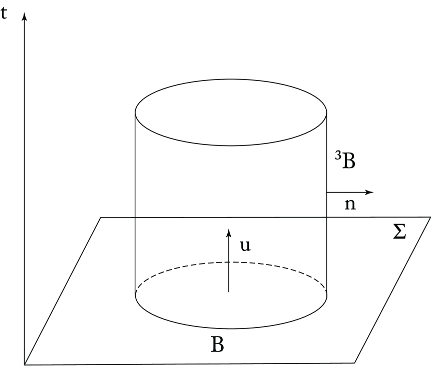
Figure 1: The time evolution of $B$ is ${}^{3}B$. Their unit normal is $n^{\mu}$ in both cases. The unit normal of a time-slice $\Sigma$ embedded in the four-dimensional manifold M is denoted by $u^{\mu}$. Note that one dimension has been suppressed, i.e. the boundary $B$ which is shown as a one-dimensional line represents a two-dimensional boundary.

Integrating the unreferenced Brown-York stress-energy-momentum surface density tensor

$$\tau^{ij}_{1} = -\frac{1}{\kappa}\left(\Theta\gamma^{ij}-\Theta^{ij}\right)$$ (1)

over the surface $B$ we obtain the unreferenced QLE

$$E_{1}=\frac{1}{\kappa}\int_{B}d^{2}x\sqrt{\sigma}u_{i}u_{j}\tau^{ij}_{1}$$ (2)

Here, the extrinsic curvature of ${}^{3}B$ as embedded in $M$ is $\Theta_{\mu\nu}=-\gamma_{\mu}^{\lambda}\nabla_{\lambda}n_{\nu}$ and the surface gravity is $\kappa=8\pi$. $\sigma_{\mu\nu}=g_{\mu\nu}-n_{\mu}n_{\nu}+u_{\mu}u_{\nu}$ is the induced metric of $B$ embedded in $\Sigma$ and its determinant is denoted by $\sigma$. Unreferenced quantities are denoted by the label ”1”. The integral is taken over $B$ at two different times $t_{f}$ and $t_{i}$ to compute the change in energy content.

Geometrized units with $G=c=1$ will be used throughout the text.

III Computation of the QLE for the FLRW metric

The Brown-York QLE Brown:1992br of the FLRW metric given by

$$ds^{2}=-dt^{2}+a^{2}(t)\left[\frac{1}{1-kr^{2}}dr^{2}+r^{2}d\theta^{2}+r^{2}\sin^{2}\theta d\phi^{2}\right]$$ (3)

can easily be computed Afshar_2009 ; Oltean:2020dvx where $k$ is either smaller than zero, zero or larger than zero depending on whether the universe is open, flat or closed, respectively. $a(t)$ is the usual scale factor. With the unit vectors

$$u^{\mu}=\delta_{t}^{\mu}$$ (4)

and

$$n^{\mu}=\sqrt{\frac{1-kr^{2}}{a^{2}(t)}}\delta_{r}^{\mu}$$ (5)

which satisfy the conditions $u_{\mu}u^{\mu}=-1$, $n_{\mu}n^{\mu}=1$ and $u_{\mu}n^{\mu}=0$ we obtain for the unreferenced QLE contained in a region bounded by a surface with fixed $r$

$$E_{1}=-\left|a(t)\right|r\sqrt{1-kr^{2}}$$ (6)

IV Conservation of Quasi-Local Energy

The QLE satisfies the following relation which is the closest to a conservation law which is known Schmekel:2018wbl ; AndyPrivate

$$\int_{t_{i}\cap^{3}B}^{t_{f}\cap^{3}B}d^{2}x\sqrt{\sigma}u_{i}u_{j}\tau^{ij}= - \int_{{}^{3}B}d^{3}x\sqrt{-\gamma}\tau^{ij}\mathcal{D}_{i}u_{j}$$ (7)

$$+ \int_{{}^{3}B}d^{3}x\sqrt{-\gamma}u_{\mu}n_{\nu}T^{\mu\nu}$$

A change in QLE is seen to equal the sum of two surface integrals. Whereas the second term on the right hand side of eqn. 7 can easily be recognized as a flux of ordinary stress-energy through ${}^{3}B$ the physical interpretation of $\tau^{ij}\mathcal{D}_{i}u_{j}$ may not be immediately obvious. Employing the expression for the quasilocal surface stress-energy-momentum tensor, the product rule and orthogonality conditions we obtain Schmekel:2018bcf

$$- \int_{{}^{3}B}d^{3}x\sqrt{-\gamma}\tau^{ij}\mathcal{D}_{i}u_{j}=$$

$$+ \frac{1}{\kappa}\int_{{}^{3}B}d^{3}x\sqrt{-\gamma}\nabla_{k}\left[\left(\mathcal{D}_{i}u_{j}\right)\left(\gamma^{ij}\gamma^{kl}-\gamma^{ik}\gamma^{jl}\right)\right]n_{l}$$

Thus, this term also represents a flux through ${}^{3}B$. There is evidence this flux can indeed be regarded as a flux of gravitational field energy.

In the small sphere limit the QLE as well as its time difference can be expressed in terms of contractions of $T^{\mu\nu}$ with $u_{\mu}u_{\nu}$ and $u_{\mu}n_{\nu}$, respectively, to lowest order Brown:1998bt ; Schmekel:2018bcf . This makes sense because of the absence of local gravitational field energy. In the absence of matter the lowest order terms can be expressed in terms of the Bel-Robinson tensor. Also, it is interesting to note that the structure of the term in brackets in eqn. LABEL:FieldEnergyTerm resembles the Landau-Lifshitz pseudotensor with the metric being replaced by the induced metric on the boundary ${}^{3}B$ Schmekel:2018wbl . A direct selection of the ”energy-flux component” by projecting $\tau^{ij}$ onto $u_{i}n_{j}$ is not possible, though, since the quasilocal quantities are missing normal components. Being defined as surface densities and not as volume densities conceptually the integration over the radial coordinate has already been taken place.

If the region of interest is neither small nor the contained fields are weak the following hypothetical process may serve to illustrate that eqn. LABEL:FieldEnergyTerm ought to be regarded as an energy flux of the gravitational field. The QLE on the left hand side of eqn. 7 is supposed to increase due to an increase in field energy. Instead of the latter entering the region ${}^{3}B$ we let a stream of particles cross the boundary which upon entering decay into field energy immediately. If our hypothetical particle flux $T^{\mu\nu}_{F}$ satisfies $u_{\mu}n_{\nu}T^{\mu\nu}_{\rm F}=-\tau^{ij}\mathcal{D}_{i}u_{j}$ it would offset the missing flux of field energy with the QLE increasing by the same amount. Therefore, particles (and their kinetic energy) can be converted into field energy and vice versa with the QLE being unable to distinguish between the two.

An interpretation of the conservation of quasilocal momentum and angular momentum in terms of quasilocal quantities can be found in Epp:2013hua .

V Application to the FLRW-metric

For a cosmological model with a stress energy tensor of the perfect fluid form $T_{\mu\nu}=\left(\rho+p\right)u_{\mu}u_{\nu}+pg_{\mu\nu}$ the stress-energy flux vanishes. Computing the field energy term eqn. LABEL:FieldEnergyTerm we obtain

$$E_{1}(t_{f})-E_{1}(t_{i})=-\left.\left|a(t)\right|\cdot r\sqrt{1-kr^{2}}\right|^{t_{f}}_{t_{i}}$$ (9)

where

$$\tau^{ij}\mathcal{D}_{i}u_{j}=\frac{1}{4\pi}\frac{\dot{a}(t)}{a^{2}(t)}r^{-1}{\rm sgn}\left(a(t)\right)\sqrt{1-kr^{2}}$$ (10)

The integral can be evaluated with $\sqrt{-\gamma}=r^{2}a^{2}(t)\sin\theta$. Therefore, conservation of energy as provided by eqn. 7 holds.

VI Conclusions

Given the definition of quasilocal energy by Brown and York and the conservation of quasilocal energy given in eqn. 7 the QLE can be regarded to be conserved in the sense that a change in QLE must be caused by a flux of ordinary stress-energy or field energy or by a suitable combination thereof.

Considering a topologically spherical region of constant $r$ in a flat FLRW-universe the energy contained within the sphere is proportional to $\left|a(t)\right|$ with the change in the contained energy being compensated by an appropriate flux into or out of $B$. The exact nature and origin of this flux has presently to be considered unknown. Yet, the formalism of QLE indicates it has to exist since the FLRW-metric is a solution of the Einstein field equations.

However, keep in mind that when changing from comoving to proper distance in a flat universe with $d(t)=ra(t)$ eqn. 6 predicts a constant value when $d(t)$ is fixed, so the flux is an observer-dependent effect as could have been expected. Thus, an incoming energy flux seen by some observers can be linked to a change in the background geometry in that frame.

Appendix A Intermediate Results

We list the non-vanishing components of the extrinsic curvature and the stress-energy-momentum surface density tensor

$$\Theta^{\theta}_{\theta}=\Theta^{\phi}_{\phi}=-\frac{\sqrt{1-kr^{2}}}{r\left|a(t)\right|}$$ (11)

$$\tau^{\theta\theta}=\frac{\sqrt{1-kr^{2}}}{\kappa r^{3}\left|a^{3}(t)\right|}$$ (12)

$$\tau^{\phi\phi}=\frac{\sqrt{1-kr^{2}}}{\kappa r^{3}\left|a^{3}(t)\right|\sin^{2}\theta}$$ (13)

$$\tau^{tt}=-\frac{2\sqrt{1-kr^{2}}}{\kappa r\left|a(t)\right|}$$ (14)