On the statistical stability of families of attracting sets and the contracting Lorenz attractor

Abstract.

We present criteria for statistical stability of attracting sets for vector fields using dynamical conditions on the corresponding generated flows. These conditions are easily verified for all singular-hyperbolic attracting sets of $C^{2}$ vector fields using known results, providing robust examples of statistically stable singular attracting sets (encompassing in particular the Lorenz and geometrical Lorenz attractors). These conditions are shown to hold also on the persistent but non-robust family of contracting Lorenz flows (also known as Rovella attractors), providing examples of statistical stability among members of non-open families of dynamical systems. In both instances, our conditions avoid the use of detailed information about perturbations of the one-dimensional induced dynamics on specially chosen Poincaré sections.

1. Introduction

The statistical viewpoint on Dynamical Systems is one of the cornerstones of most recent developments in dynamics. Given a flow $\phi_{t}$ on a manifold $M$, a central concept is that of physical measure, a $\phi_{t}$-invariant probability measure $\mu$ whose ergodic basin

$$B(\mu)=\left\{x\in M:\frac{1}{T}\int_{0}^{T}\varphi(\phi_{t}x)\,dt\to\int\varphi\,d\mu\mbox{ for all continuous }\varphi:M\to{\mathbb{R}}\right\}$$

has positive volume or Lebesgue measure, which we write $\operatorname{Leb}$ and take as the measure associated with any non-vanishing volume form on $M$.

This kind of measure provides asymptotic information on a set of trajectories that one hopes is large enough to be observable in real-world models.

The stability of physical measures under small variations of the map allows for small errors on the formulation of the transformation law governing the dynamics not to disturb too much the long term behavior, as measured by the most basic statistical data provided by asymptotic time averages of continuous functions along orbits. In principle when considering practical systems we cannot avoid external noise, so every realistic mathematical model should exhibit these stability features to be able to cope with unavoidable uncertainty about the “correct” parameter values, observed initial states and even the specific mathematical formulation involved.

In this note we explicitly state criteria for statistical stability of families of continuous dynamical systems (flows generated by vector fields) exhibiting not necessarily robust features (that is, the family needs not be open in a smooth topology of vector fields or flows) given by singular attracting sets, namely singular-hyperbolic or contracting Lorenz models. These families of invariant sets, containing regular trajectories accumulating equilibria are not structurally stable, that is, cannot be seen as different realizations of the same system under a continuous change of coordinates; see e.g. [26]. However, using physical measures we can obtain stability in a statistical sense: asymptotical time averages of continuous observables over most trajectores will vary continuously with the underlying dynamical system.

We first apply the criteria to obtain a rather geometrical proof of statistical stability for open families singular-hyperbolic (or Lorenz-like) attracting sets, encompassing in particular de classical Lorenz attractor and also the family of geometrical Lorenz attractors; see [15] for a presentation of these systems. Our proof for these systems takes advantage of already known results. Secondly, we show that the non-open, but persistent, Rovella family ${\mathcal{G}}:X\to{\mathcal{X}}^{3}({\mathbb{R}}^{3})$ of perturbation of the contracting Lorenz attractor [42] also satisfies the criteria, where $X$ is a metric space and ${\mathcal{G}}$ is continuous with respect to the $C^{3}$ topology among smooth vector filds of ${\mathbb{R}}^{3}$. Thus, the physical measures on these attractors are statistically stable within the family, that is, when considering perturbations along the image of the family ${\mathcal{G}}$. We note that recently Alves-Khan [5] showed that contracting Lorenz flows are statistically unstable if we consider all the nearby flows in the $C^{3}$ topology, that is, we replace $X$ by an open subset $U$ of ${\mathcal{X}}^{3}({\mathbb{R}}^{3})$ containg the contracting Lorenz attractor.

Another notion of stability is that of stochastic stability, dealing with small random perturbations along each trajectory, which we do not consider here, but was studies for sectional-hyperbolic and contracting Lorenz attractors by Metzger and Morales [33, 34].

Our criteria do not assume uniqueness of the physical measure supported on the attracting set: we deal with an at most countable family of ergodic physical measures, as long as their ergodic basins contain $\operatorname{Leb}$-almost all points whose trajectories accumulate on the attracting set. Moreover, the criteria do not involve the statistical stability of a one-dimensional quotient map induced by a certain Poincaré return map, defined by a suitable choice of global cross-section, as in the case of the previous works on statistical stability of geometric Lorenz attractors of Alves-Soufi [2] and Bahsoum-Ruziboev [20]. Our criteria are a mix of dynamical (robust expansiveness) and thermodynamical (physical measures satisfy the Entropy Formula) properties of the flow restricted to the attracting set and its perturbations.

We mention that statistical stability and other strong properties of the one-dimensional quotient maps (contracting Lorenz maps) mentioned above for the Rovella attractor were obtained by Metzger [32] and Alves-Soufi [6]. Decay of correlations and other statistical properties for the Poincaré return map were obtained more recently by Galatolo-Nisoli-Pacifico [24], and a Thermodynamical Formalism for the contracting Lorenz flow was developed by Pacifico-Todd [37].

Our results can be immediately applied to certain known families of bifurcations giving rise to attractors belonging to these two classes: see e.g. [41, 35, 36]. The family of systems obtained after the unfolding of these bifurcation scenarios exhibiting singular-hyperbolic (Lorenz-like) or contracting Lorenz attractors are automatically statistically stable.

Similar ideas to the criteria presented here, exploring consequences of the characterization of invariant measures satisfying the Entropy Formula [28] were already used to deal with stochastic and statistical stability of uniformly and non-uniformly expanding maps; see e.g. [27, 18, 19] and [7]. A natural notion of stability for maps with several physical measures supported on a given attracting set was provided in [3]. The same strategy was applied to obtain statistical stability for sectional-hyperbolic attracting sets (a higher (co)dimensional extension of the notion of singular-hyperbolicity) in [8], where the focus lies on the technically much harder task of deducing the properties needed to apply the criteria, due to the high dimensionality of the objects involved.

1.1. Statements of the results

Let $M$ be a compact connected Riemannian manifold with dimension $\dim M=m$, induced distance $d$ and volume form $\operatorname{Leb}$. Let ${\mathcal{X}}^{r}(M)$, $r\geq 1$, be the set of $C^{r}$ vector fields on $M$ endowed with the $C^{r}$ topology and denote by $\phi_{t}$ the flow generated by $G\in{\mathcal{X}}^{r}(M)$.

1.1.1. Preliminary definitions

An invariant set $\Lambda$ for the flow $\phi_{t}$ generated by the vector field $G\in{\mathcal{X}}^{r}(M)$, for some fixed $r\geq 2$, is a subset of $M$ which satisfies $\phi_{t}(\Lambda)=\Lambda$ for all $t\in{\mathbb{R}}$. Given a compact invariant set $\Lambda$ for $G\in{\mathcal{X}}^{r}(M)$, we say that $\Lambda$ is isolated if there exists an open set $U\supset\Lambda$ such that $\Lambda=\bigcap_{t\in{\mathbb{R}}}\operatorname{Closure}{\phi_{t}(U)}$. If $U$ can be chosen so that $\operatorname{Closure}{\phi_{t}(U)}\subset U$ for all $t>0$, then we say that $\Lambda$ is an attracting set and $U$ a trapping region (or isolated neighborhood) for $\Lambda=\Lambda_{G}(U)=\cap_{t>0}\operatorname{Closure}{\phi_{t}(U)}$.

We note that every attracting set admits a natural continuation, since there exists a neighborhood ${\mathcal{V}}$ of $G$ in ${\mathcal{X}}^{r}(M)$ so that $\operatorname{Closure}{\phi^{Y}_{t}}(U)\subset U$ for all $t>0$ and each $Y\in{\mathcal{V}}$, where $(\phi_{t}^{Y})_{t\in{\mathbb{R}}}$ is the flow generated by $Y$, and so we may consider the attracting set $\Lambda_{Y}(U)$.

Physical measures are related to equilibrium states of a certain potential function. Let $\psi:M\rightarrow{\mathbb{R}}$ be a continuous function. Then a $\phi_{t}$-invariant probability measure $\mu$ is a equilibrium state for the potential $\psi$ if

$$P_{G}(\psi)=h_{\mu}(\phi_{1})+\int\psi\,d\mu,\quad\mbox{where}\quad P_{G}(\psi)=\sup_{\nu\in{\mathcal{M}}}\left\{h_{\nu}(\phi_{1})+\int\psi\,d\nu\right\},$$

and ${\mathcal{M}}$ is the set of all $\phi_{t}$-invariant probability measures. The quantity $P_{G}(\phi)$ is called the Topological Pressure and the identity on the right hand side is a consequence of the Variational Principle; see e.g. [44] for definitions of entropy $h_{\mu}(\phi_{1})$ and topological pressure $P_{G}(\psi)$.

A sign of chaoticity in an attracting set of a vector field is the property of expansiveness. Denote by $S({\mathbb{R}})$ the set of surjective increasing continuous functions $h:{\mathbb{R}}\to{\mathbb{R}}$. We say that the flow is expansive if for every $\varepsilon>0$ there is $\delta>0$ such that, for any $h\in S({\mathbb{R}})$

$$d(\phi_{t}(x),\phi_{h(t)}(y))\leq\delta,\quad\forall t\in{\mathbb{R}}\implies\exists t_{0}\in{\mathbb{R}}\text{ such that }\phi_{h(t_{0})}(y)\in\phi_{[t_{0}-\varepsilon,t_{0}+\varepsilon]}(x).$$

We say that a invariant compact set $\Lambda$ is expansive if the restriction of $\phi_{t}$ to $\Lambda$ is an expansive flow.

Robust properties are extremely important in Dynamical Systems theory. To precisely state the main result, we now define robust expansiveness. Let ${\mathcal{G}}:X\to{\mathcal{X}}^{r}(M)$ be a continuous family of vector fields, where $r\geq 2$ is fixed and $X$ is a metric space. We write $G_{s}={\mathcal{G}}(s)$ the vector field given by $s\in X$ and denote by $(\phi_{t}^{G_{s}})_{t\in{\mathbb{R}}}$ the corresponding flow in what follows.

We say that the family ${\mathcal{G}}$ of vector fields is robustly expansive on an attracting set $\Lambda=\cap_{t>0}\operatorname{Closure}{\phi^{G_{s}}_{t}(U})$ for some $s\in X$ if there exists a neighborhood $N$ of $s$ in $X$ such that for every $\varepsilon>0$ there is $\delta>0$ such that, for any $x,y\in\Lambda_{s}=\cap_{t>0}\operatorname{Closure}{\phi^{G_{s}}_{t}(U)}$, $h\in S({\mathbb{R}})$ and $s\in V$

$$d(\phi^{G_{s}}_{t}(x),\phi^{G_{s}}_{h(t)}(y))\leq\delta,\quad\forall t\in{\mathbb{R}}\implies\exists t_{0}\in{\mathbb{R}}\text{ such that }\phi_{h(t_{0})}(y)\in\phi^{G_{s}}_{[t_{0}-\varepsilon,t_{0}+\varepsilon]}(x).$$

1.1.2. Statistical stability of equilibrium states

We can now precisely state our criteria for statistical stability of families of attracting sets of vector fields.

Theorem A.

Let us assume that the family ${\mathcal{G}}$ admits a trapping region $U$ so that the attracting set $\Lambda_{s}(U)=\cap_{t>0}\operatorname{Closure}{\phi_{t}^{G_{s}}(U)}$ satisfies, for each parameter $s$ in some subset $N\subset X$:

1. there are finitely many ergodic physical measures $\mu^{s}_{i},1\leq i\leq k_{i}$ supported in $\Lambda_{s}$ so that $\operatorname{Leb}\big{(}U\setminus\sum_{i}B(\mu_{i}^{s})\big{)}=0$;

2. there exists a family of potentials $\psi_{s}:\Lambda_{s}\to{\mathbb{R}}$ so that $\mu$ is an equilibrium state w.r.t. $\psi_{s}$, i.e. $0=h_{\mu}(\phi_{1}^{G_{s}})+\int\psi_{s}\,d\mu$ if, and only if, $\mu$ a physical measure;

3. the function $\Psi:W(U):=\{(s,x)\in N\times U:x\in\Lambda_{s}(U)\}\to{\mathbb{R}}$ given by $\Psi(s,x)=\psi_{s}(x)$ is continuous; and

4. the family ${\mathcal{G}}$ is robustly expansive.

Then, for each converging sequence $s_{n}\in N$ to $s\in N$ and every choice $\mu^{s_{n}}$ of a physical measure supported on $\Lambda_{s_{n}}(U)$, every weak^∗ accumulation point $\mu$ of $(\mu^{s_{n}})_{n\geq 1}$ is a convex linear combination of the ergodic physical measures of $\Lambda_{s}(U)$.

The conclusion of the previous theorem means, more precisely, that

1. there are weights $\alpha_{i}\geq 0$ such that $\sum_{i}\alpha_{i}=1$ and $\mu=\sum_{i}\alpha_{i}\mu_{i}^{s}$; and

2. we have $\left|\int{\varphi}\,d\mu_{n}-\sum_{i}\alpha_{i}\int{\varphi}\,d\mu_{i}^{s}\right|\xrightarrow[n\to\infty]{}0$ for every continuous observable ${\varphi}:U\to{\mathbb{R}}$.

In the applications which we present in what follows, the property stated in item (2) above is provided by the (Pesin’s) Entropy Formula [40, 30, 28], that is, the potential is a geometric potential $\psi_{s}=\log|\det|D\psi_{1}^{G_{s}}\mid E^{cu}|$ where $E^{cu}$ is a certain continuous subbundle of the tangent bundle at the points of the attracting set.

1.2. Application to singular-hyperbolic attracting sets

Here we provide open classes of examples of application of the previous abstract setting: the singular-hyperbolic attracing sets (also known as “Lorenz-like attractors”), encompassing, as particular cases, the classical Lorenz attractor and the geometric Lorenz attractor.

1.2.1. Background on singular-hyperbolicity

Let $\Lambda$ be a compact invariant set for $G\in{\mathcal{X}}^{r}(M)$. We say that $\Lambda$ is partially hyperbolic if the tangent bundle over $\Lambda$ can be written as a continuous $D\phi_{t}$-invariant sum $T_{\Lambda}M=E^{s}\oplus E^{cu},$ where $d_{s}=\dim E^{s}_{x}\geq 1$ and $d_{cu}=\dim E^{cu}_{x}=2$ for $x\in\Lambda$, and there exist constants $C>0$, $\lambda\in(0,1)$ such that for all $x\in\Lambda$, $t\geq 0$, we have

• uniform contraction along $E^{s}$: $\|D\phi_{t}|E^{s}_{x}\|\leq C\lambda^{t};$

• domination of the splitting: $\|D\phi_{t}|E^{s}_{x}\|\cdot\|D\phi_{-t}|E^{cu}_{\phi_{t}x}\|\leq C\lambda^{t}.$

We refer to $E^{s}$ as the stable bundle and to $E^{cu}$ as the center-unstable bundle. A partially hyperbolic attracting set is a partially hyperbolic set that is also an attracting set.

The center-unstable bundle $E^{cu}$ is volume expanding if there exists $K,\theta>0$ such that $|\det(D\phi_{t}|E^{cu}_{x})|\geq Ke^{\theta t}$ for all $x\in\Lambda$, $t\geq 0$.

We say that $\sigma\in M$ with $G(\sigma)=0$ is an equilibrium or singularity. In what follows and we denote by $\operatorname{Sing}(G)$ the family of all such points. We say that a singularity $\sigma\in\operatorname{Sing}(G)$ is hyperbolic if all the eigenvalues of $DG(\sigma)$ have non-zero real part.

A point $p\in M$ is periodic for the flow $\phi_{t}$ generated by $G$ if $G(p)\neq\vec{0}$ and there exists $\tau>0$ so that $\phi_{\tau}(p)=p$; its orbit ${\mathcal{O}}_{G}(p)=\phi_{{\mathbb{R}}}(p)=\phi_{[0,\tau]}(p)=\{\phi_{t}p:t\in[0,\tau]\}$ is a periodic orbit, an invariant simple closed curve for the flow. An invariant set is nontrivial if it is neither a periodic orbit nor an equilibrium.

We say that a compact nontrivial invariant set $\Lambda$ is a singular hyperbolic set if all equilibria in $\Lambda$ are hyperbolic, and $\Lambda$ is partially hyperbolic with volume expanding center-unstable bundle. A singular hyperbolic set which is also an attracting set is called a singular hyperbolic attracting set. An attractor is a transitive attracting set, that is, an attracting set $\Lambda$ with a point $z\in\Lambda$ so that its $\omega$-limit

$$\omega(z)=\left\{y\in M:\exists t_{n}\nearrow\infty\text{ s.t. }\phi_{t_{n}}z\xrightarrow[n\to\infty]{}y\right\}$$

coincides with $\Lambda$.

1.2.2. Singular-hyperbolicity and statistical stability

We may now state the following.

Corollary B.

Every singular-hyperbolic attracting set for a $C^{2}$ flow admits a neighborhood ${\mathcal{V}}$ in ${\mathcal{X}}^{2}(M)$ where every system is statistically stable.

More precisely, given a flow $G$ of class $C^{2}$ on a compact manifold exhibiting a singular-hyperbolic attracting set $\Lambda$, then we can find a neighborhood ${\mathcal{V}}$ of $G$ in ${\mathcal{X}}^{2}(M)$ and a neighborhood $U$ of $\Lambda$ so that, letting ${\mathcal{G}}:{\mathcal{V}}\to{\mathcal{X}}^{2}(M)$ be the restriction of the identity to ${\mathcal{V}}$, then ${\mathcal{G}}$ satisfies the conditions of Theorem A. Indeed: for each $Y\in{\mathcal{V}}$ we have that $\Lambda_{Y}(U)$ is a singular-hyperbolic attracting set and

1. $\Psi(Y,x)=\log|\det D\phi_{1}^{Y}\mid E^{cu}_{x}|,x\in\Lambda_{Y}(U)$ is continuous on $W(U)$ as in Theorem A(3) by robustness and continuity of dominated splittings in the $C^{2}$ neighborbood ${\mathcal{V}}$ – see e.g. [21, Appendix B];

2. there are finitely many ergodic physical measures $\mu^{Y}_{i},i=1,\dots,k(Y)$ supported in $\Lambda_{Y}(U)$ whose basins cover a full volume subset of $U$ – see e.g. [17, 13];

3. each physical measure supported in $\Lambda_{Y}(U)$ is an equilibrium state with respect to the potential $\psi_{Y}(x)=\psi(Y,x)$ – see e.g. [17] again; and

4. ${\mathcal{G}}$ is robustly expansive: this was recently obtained in [10].

In the particular case of the classical Lorenz attractor [29], which was shown to be a robustly transitive singular-hyperbolic attractor with the features of the geometrical Lorenz attractor [43], we have a unique physical measure which has strong statistical properties [16, 14, 11] on a $C^{2}$ neighborhood ${\mathcal{V}}$ as above. That is, we have (1-4) with $k(Y)\equiv 1$. Hence we reobtain a version of the main result of [20]:

Corollary 1.1.

In a $C^{2}$ neighborhood ${\mathcal{V}}$ of a geometric Lorenz attractor with trapping region $U\subset{\mathbb{R}}^{3}$, if $Y_{n}\to Y$ in the $C^{2}$ topology of ${\mathcal{X}}^{2}({\mathbb{R}}^{3})$, then the unique physical measures supported on the attractors satisfy $\lim_{n\to\infty}\int{\varphi}\,d\mu_{Y_{n}}=\int{\varphi}\,d\mu_{Y}$ for all continuous observables ${\varphi}:U\to{\mathbb{R}}$.

1.3. Application to the Contracting Lorenz (Rovella) attractor

Here we provide a non-trivial example of application of the abstract setting of the Main Theorem where the family of dynamics is not open: perturbation of the Rovella or Contracting Lorenz attractors, presented by Rovella in [42].

1.3.1. Background on the contracting Lorenz attractor

To present this dynamics and its main features, we start with the geometric contracting Lorenz Flow, which is a modification of the geometric Lorenz attractor from [25, 26, 1], in which the uniformly expanding direction at the singularity is replaced by a strict nonuniformly expanding direction. In broad terms, following [37, 24], we start with a linear vector field $(\dot{x},\dot{y},\dot{z})=(\lambda_{1}x,\lambda_{2}y,\lambda_{3}z)$ in the cube $[-1,1]^{3}$ whose real eigenvalues $\lambda_{1},\lambda_{2},\lambda_{3}$ of the singularity at the origin satisfy

$$-\lambda_{2}>-\lambda_{3}>\lambda_{1}>0,\quad r=-\frac{\lambda_{2}}{\lambda_{1}},\quad s=-\frac{\lambda_{3}}{\lambda_{1}},\quad\text{and}\quad r>s+3.$$

We note that $\lambda_{1}+\lambda_{3}<0$ while in the geometric Lorenz attractor the construction starts with $\lambda_{1}+\lambda_{3}>0$; see e.g. [15, Chapter 3, Section 3].

Setting $\Sigma^{-}=[-1/2,0]\times[-1/2,1/2]\times\{1\};\Sigma^{+}=[0,1/2]\times[-1/2,1/2]\times\{1\}$; and $\Sigma=\Sigma^{+}\cup\Sigma^{-}$ we have a cross-section for the linear flow; see the left hand side of Figure 1. It is straightforward to calculate the Poincaré map from $\Sigma^{\pm}$ to the cross-section $x=\pm 1$: for the $+$ case we obtain $(x,y,1)\mapsto(1,yx^{r},x^{s})$.

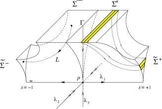
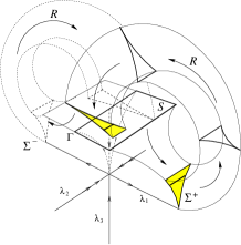
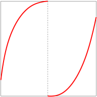
Figure 1. Sketch of behaviour of the linear flow near the origin, on the left hand side; and the behaviour of the flow in a neighborhood of the attractor, on the center; and the one-dimensional map $T_{0}$ on the right hand side.

Outside the cube, we obtain a butterfly shape for the attractor after rotating the orbits around the origin and returning to $\Sigma$, by a suitable composition of a rotation, an expansion and a translation; see the center of Figure 1 and for more details, see e.g. [15, Chapter 3, Section 3].

Remark 1.2.

As shown in [42] the condition $r>s+3$ ensures the existence of a $C^{3}$ uniformly contracting stable foliation for the Poincaré first return map of all small enough perturbations of the contracting geometric Lorenz flow.

Using this foliation it is possible to obtain an explicit expression for the Poincaré first return map $R_{0}(x,y)=(T_{0}x,H_{0}(x,y))$ where

$$T_{0}(x)=\operatorname{sgn}(x)\cdot(-\rho|x|^{s}+1/2)\quad\text{and}\quad H_{0}(x,y)=\operatorname{sgn}(x)\cdot(y|x|^{r}+c)$$

for some $c>0$ depending on the choice of the rotations and translations (assumming some symmetry to simplify the exposition), $r$ and $s$ are as defined above, and $0<\rho\leq(1/2)^{-s}$.

In [42, Item 4, page 240] it is shown that $T_{0}$ satisfies (see the right hand side of Figure 1)

1. $T_{0}$ is piecewise $C^{3}$ with two branches, restricted to each it is onto, and $T_{0}^{\prime}(x)=O(x^{s-1})$ at $x=0$ where $s-1>0$;

2. $T_{0}(0^{+})=1/2$ and $T_{0}(0^{-})=-1/2$;

3. $T_{0}^{\prime}<0$ on $[-1/2,1/2]\setminus\{0\}$;

4. $\max T_{0}^{\prime}\mid_{(0,1/2]}=T_{0}^{\prime}(1/2)$ and $\max T_{0}^{\prime}\mid_{[-1/2,0)}=T_{0}^{\prime}(-1/2)$.

   Moreover, there are values of $\rho\leq(1/2)^{-s}$ so that

5. $\pm 1/2$ are preperiodic repelling for $T_{0}$; and

6. $T_{0}$ has negative Schwarzian derivative.

Rovella established that the flow of the vector field $G_{0}$ with these features has an attractor $\Lambda_{0}$ and studied the dynamics of the perturbations of this flow. To state the results more relevant to us, we present the notion of measure theoretical stability (persistence) among parametrized families of systems.

We recall that a point $x$ is a density point of a subset $S$ of a finite dimensional Riemannian manifold $M$, if

$$\lim_{r\to 0}\frac{\operatorname{Leb}(B_{r}(x)\cap S)}{\operatorname{Leb}(B_{r}(x))}=1,$$

where $B_{r}(x)$ the ball of radius $r$ centered at $x$.

Definition 1.

Given a subset $S$ of a Banach space $X$, we say that $x\in S$ is a point of $k$-dimensional full density of $S$ if there exists a $C^{\infty}$ submanifold $N\subset X$ with codimension $k$, containing $x$, such that every $k$-dimensional manifold $M$ intersecting $N$ transversally at $x$ admits $x$ as a full density point of $S\cap M$ in $M$.

We may now state what is mean by a persistent attractor.

Definition 2.

An attractor $\Lambda$ of a vector field $X\in{\mathcal{X}}^{\infty}$ is $k$-dimensionally almost persistent if it has a local basin $U$ such that $X$ is a $k$-dimensional full density point of the set of vector fields $Y\in{\mathcal{X}}^{\infty}$, for which $\Lambda_{Y}=\cap_{t>0}Y^{t}(U)$ is an attractor.

In [42, item (b) at page 235] it is stated (and later proved in the same work) that the attractor $\Lambda_{0}$ constructed as above is $2$-dimensionally almost persistent in the $C^{3}$ topology. Recently this attractor was shown to be a prototype of a class of invariant sets, similarly to the geometric Lorenz attractor, which is a prototype of a singular-hyperbolic set.

Definition 3.

A compact invariant partially hyperbolic set $\Lambda$ of a vector field $G$ (in the same setting as subsection 1.2.1, i.e. $d_{cu}=2$), whose singularities are hyperbolic, is asymptotically sectional hyperbolic if the center-unstable subbundle is eventually asymptotically expanding outside the stable manifold of the singularities. That is, there exists $c_{*}>0$ so that

$$\limsup_{T\to\infty}\frac{1}{T}\log|\det(D\phi_{T}\mid E^{cu}_{x})|\geq c_{*},\quad\text{for each }x\in\Lambda\setminus\bigcup_{\sigma\in\Lambda\cap\operatorname{Sing}(G)}W^{s}(\sigma).$$

Here $W^{s}(\sigma)=\{x\in M:\lim_{t\to+\infty}\phi_{t}x=\sigma\}$ is the stable manifold of the hyperbolic equilibrium $\sigma$. It is well-known that $W^{s}(\sigma)$ is a immersed submanifold of $M$; see e.g.[38].

The following was recently proved in [31].

Theorem 1.3.

The attractor $\Lambda_{0}$ is $2$-dimensionally almost persistent asymptotically sectional hyperbolic in the $C^{3}$ topology.

Let $R\subset{\mathcal{X}}^{3}({\mathbb{R}}^{3})$ be the set of vector fields exhibiting a Rovella attractor provided by Theorem 1.3 and ${\mathcal{G}}:R\to{\mathcal{X}}^{3}({\mathbb{R}}^{3})$ be the restriction of the identity to $R$.

Theorem C.

The family ${\mathcal{G}}$ of contracting Lorenz attractors, with trapping region $U$, is such that each of its elements admits a unique physical measure, whose basin covers $U$ except for zero $\operatorname{Leb}$-measure subset and is statistically stable.

1.4. Organization of the text

The strategy of the proof of Theorem C is to show that ${\mathcal{G}}$ above satisfies all the conditions of Theorem A with uniqueness of physical measures for each attractor. This is presented in Section 2. In Section 3 we provide a proof of Theorem A.

Acknowledgments

I thank the Mathematics Department at UFBA; CAPES-Brazil and CNPq-Brazil for the basic support of research activities; and also the anonymous referee for many suggestions that helped to improve the text.

2. The contracting Lorenz family of attractors

Here we prove Theorem C by showing that the family perturbations of the attractor $\Lambda_{0}$ introduced by Rovella, known also as contracting Lorenz attractors, satisfies the conditions for statistical stability in the weak^∗ topology stated in Theorem A, with unique physical measures for each element of the family ${\mathcal{G}}$ in the statement of Theorem C.

2.1. Existence and uniqueness of physical measure

We start by observing that the partial hyperbolicity of the family of contracting Lorenz flows given by 1.3 implies that there exists an $D\phi_{t}$-invariant and uniformly contracting extension of the subbundle $E^{s}$ to $U$ (which we denote by the same symbol) together with $\varepsilon_{0}>0$ such that, for all points $x\in U$ and $0<\varepsilon<\varepsilon_{0}$, there exists a $C^{3}$ embedded disk

$$W^{ss}_{\varepsilon}(x)=\{y\in B(x,\varepsilon):d(\phi_{t}y,\phi_{t}x)\xrightarrow[t\to+\infty]{}0\}$$

which satisfies $T_{x}W^{s}_{\varepsilon}(x)=E^{s}_{x}$ and is $\phi_{t}$-invariant, that is $\phi_{t}W^{s}_{\varepsilon}(x)\subset W^{s}_{\varepsilon}(\phi_{t}x)$ for all $t>0$; see [12]. In what follows, this disk is the local (strong-)stable manifold of size $\varepsilon$ of $x$ and, when we do not want to specify its size, we write $W^{s}_{loc}(x)$ understanding that the size is to be taken uniform in $U$. It follows from the theory of uniform hyperbolicity that $\varepsilon_{0}>0$ above may be taken uniformly on $U$ and on the vector field $G$ on a neighborhood ${\mathcal{V}}$ of $G_{0}$; see [38].

Using the results from [42], we have that, in a $C^{3}$ neighborhood ${\mathcal{V}}$ of the vector field $G_{0}$ described in Subsection 1.3.1, the Poincaré first return map $R_{G}$ to the cross-section $\Sigma$ for each $G\in{\mathcal{V}}$ can be written as a skew-product $R_{G}(x,y)=(T_{G}x,H_{G}(x,y))$ after a suitable $C^{3}$ change of coordinates; this is a consequence of Remark 1.2.

As proved in [42], used in [32] and generalized recently in [6], there exists a one-parameter family $G_{a},a\in[0,1]$ of vector fields $C^{3}$ close to $G_{0}$ admiting a subset $E\subset(0,a_{0})$ of parameters (“Rovella parameters”) so that $0$ is a density point of $E$. Moreover, the one-dimensional map $T_{a}$ corresponding the quotient $T_{G_{a}}$ of the Poincaré return map to $\Sigma$ over the stable foliation, satisfies the following.

Theorem 2.1.

[6] For each $a\in E$, the map $T_{a}$ of the interval $[-1/2,1/2]$ is a transitive non-uniformly expanding map with slow recurrence to the critical set; and has a unique absolutely continuous ergodic invariant probability measure $\nu_{a}$, whose basin $B(\nu_{a})$ equals $[-1/2,1/2]$ except for a subset of zero Lebesgue measure.

As explained in [32, Section 7] and also e.g. in [16, Section 6], the existence of an ergodic physical measure for the quotient map $T_{a}$ of a Poincaré return map $R_{a}$ over a uniformly contracting regular foliation, induces an ergodic physical invariant probability measure for the flow through a standard procedure. In addition, if we start with a physical measure with full ergodic basin for $T_{0}$, then the induced measure also has full ergodic basin over the orbits of the flow starting on the cross-section, which we may assume without loss of generality to include $U$.

Hence, the flow of $G_{a}$ on the trapping region $U$ admits a physical invariant probability measure $\mu_{a}$ supported on $\Lambda_{a}=\Lambda_{G_{a}}(U)$ with full ergodic basin on $U$. Thus this measure is the unique physical measure on $U$. We have obtained item (1) of the statement of Theorem A with a unique measure for each element of the family ${\mathcal{G}}$.

2.2. The physical measure is a $SRB$ measure

Let $R_{a}$ be the Poincaré first return map to $\Sigma$. As presented in [16, Section 8] or [15, Chapter 7, Sections 9-11], if we assume that

• the Poincaré return map $R_{a}(x,y)=(T_{a}x,H_{a}(x,y))$ to the cross-section $\Sigma$ satisfies

  • $H_{a}(x,\cdot)$ is a uniform contraction;

  • $T_{a}$ is a one-dimensional non-uniformly expanding map with slow recurrence to the critical set (this is the discontinuous point $\{0\}$), as defined in [4, Section 5] and provided by [6];

then every absolutely continuous ergodic $T_{0}$-invariant probability measure $\nu_{a}$ induces a measure $\mu_{a}$ which is an ergodic hyperbolic $SRB$-measure. That is, $\mu_{a}$ admits an absolutely continuous disintegration along unstable manifolds.

Remark 2.2.

Observe that since the flow direction on partially hyperbolic sets is contained in the central-unstable direction (see e.g. [9, Lemma 5.1]), then Oseledets Theorem ensures that

$$\int\log|\det(D\phi_{1}^{G_{a}}\mid E^{cu})|\,d\mu_{a}=\int\lambda^{+}(x)\,d\mu_{a}(x)\geq c_{*}>0,$$

where $\lambda^{+}(x)=\lim_{T\to\infty}\frac{1}{T}\log|\det(D\phi_{T}\mid E^{cu}_{x})|$ is the largest Lyapunov exponent along the two-dimensional bundle $E^{cu}$ for $\mu_{a}$-a.e. $x$. This is strictly positive by asymptotical sectional-expansion, for otherwise a $\mu_{a}$ generic point would belong to the stable manifold of a singularity $\sigma\in\Lambda_{a}$, and thus $\mu_{a}=\delta_{\sigma}$. But this would contradict the $SRB$ property obtained above.

According the characterization of $SRB$ measures obtained by Ledrappier and Young [28] we have $h_{\mu_{a}}(\phi_{1}^{G_{a}})=\int\lambda^{+}(x)\,d\mu_{a}(x)$ and so after Remark 2.2 we see that $\mu_{a}$ satisfies the Entropy Formula

$$h_{\mu_{a}}(\phi_{1}^{G_{a}})=\int\log|\det(D\phi_{1}^{G_{a}}\mid E^{cu})|\,d\mu_{a}>0.$$ (1)

Reciprocally, an invariant probability measure $\mu$ satisfying the Entropy Formula (1) for the $C^{2}$ partially hyperbolic flow $G_{a}$ is a $SRB$ measure (by the result from [28]) and since $E^{cu}$ is two-dimensional, then $\mu$ is a hyperbolic measure: the Lyapunov exponents along $E^{s}$ are strictly negative, there exists a positive Lyapunov exponent along the $E^{cu}$ direction together with the zero exponent along the flow direction. Consequently, being a $SRB$ and hyperbolic measure, it is a physical measure; see e.g. [39, 45].

Hence, using the the potential $\psi_{a}=-\log|\det(D\phi_{1}^{G_{a}}\mid E^{cu})|$ we obtain item (2) of the statement of Theorem A.

The continuity of dominated splittings [21, Appendix B] with respect to the base point but also with respect to the dynamics, together with the $C^{3}$ smoothness of the vector fields involved, ensures that item (3) also holds in this setting.

2.3. Robust expansiveness of contracting Lorenz flows

Here we deduce robust expansiveness. We first use the following result from [32, Section 4]. We write $c_{a}^{\pm}=T_{a}(0^{\pm})=\lim_{t\to 0^{\pm}}f(t)$; see the right hand side of Figure 1. We note that $c_{a}^{-}<0<c_{a}^{+}$ and $c_{a}^{\pm}\to\pm 1/2$ when $a\to 0$.

Lemma 2.3.

[32, Lemma 4.1] There exists a $C^{3}$ neighborhood ${\mathcal{V}}$ of $G_{0}$ so that if $G_{a}\in{\mathcal{V}}$, then the map $T_{a}$ is locally eventually onto, that is, for any interval $J\subset[-1/2,1/2]\setminus\{0\}$ there exists $n=n(J)>0$ so that $f^{n}(J)\subset[c_{a}^{-},c_{a}^{+}]$.

Consequently, there does not exist a pair of points $x_{0}<y_{0}$ with the same sign in $[-1/2,1/2]\setminus\{0\}$ so that $T_{a}^{n}[x_{0},y_{0}]$ does not contain the origin for all $n\geq 1$.

We use this result to obtain robust expansiveness for the family ${\mathcal{G}}$ restricted to the neighborhood ${\mathcal{V}}$.

Let $2\delta_{0}>0$ be the distance between the cross-sections $\widetilde{\Sigma^{+}}$ and $\Sigma^{+}$, or between $\widetilde{\Sigma^{-}}$ and $\Sigma^{-}$ (they are symmetrical); see the left hand side of Figure 1. Let also $x,y\in U$ and $h:{\mathbb{R}}\to{\mathbb{R}}$ be a surjective increasing continuous function such that $d(x(t),y(t))\leq\delta$ for some $\delta\in(0,\delta_{0})$ and for all $t\in{\mathbb{R}}$, where $x(t)=\phi_{t}x$ and $y(t)=\phi_{h(t)}y$ will be the trajectories to consider in what follows (we removed $G_{a}$ from the notation of the flow to lighten the text).

We consider also the pairs of consecutive hitting times $x_{n},y_{n},n\geq 1$ of these trajectories on $\Sigma$ and their projections $\pi x_{n},\pi y_{n}$ on the quotient $[-1/2,1/2]$ of $\Sigma$ over the stable leaves.

We note that if $\pi x_{n}\cdot\pi y_{n}<0$, i.e. returns to $\Sigma$ lie on different sides with respect to the stable manifold of the singularity at the origin, then the trajectories of $x_{n}$ and $y_{n}$ will eventually separate by a distance larger than $\delta$ during their crossing of the linearized region near the singularity; see again the the left hand side of Figure 1. This would contradict the assumption on $x,y$ and $h$.

However, if we assume that $\pi x_{1}<\pi y_{1}$ and $\pi x_{1}\cdot\pi y_{1}>0$, then, because $T_{a}$ has monotonous smooth branches on $[-1/2,0)$ and $(0,1/2]$, we get $[\pi x_{j+1},\pi y_{j+1}]=T_{a}[\pi x_{j},\pi y_{j}]$ as long as $\pi x_{j}\cdot\pi y_{j}>0$ for $j=1,\dots,l$. Hence, from Lemma 2.3, the trajectories will not be in this situation for all $j\geq 1$: there exists $l>1$ so that $\pi x_{j+1}\cdot\pi y_{j+1}<0$. Hence $x,y$ cannot satisfy $\pi x_{1}\cdot\pi y_{1}<0$ nor $\pi x_{1}\neq\pi y_{1}$.

We conclude that $\pi x_{1}=\pi y_{1}$ and both trajectories share a stable leaf of the Poincaré return map $R_{a}$. This means that there exists $t_{1}>0$ and $h(s_{1})>0$ so that $x_{1}=\phi_{t_{1}}x,y_{1}=\phi_{h(s_{1})}y$ and $d(x_{1},\phi_{h(t_{1})}y)<\delta$, and also that $y_{1}$ is in the same contracting leaf of $R_{0}$ as $x_{1}$. Hence, since there exists $d>0$ so that $\|G_{a}\|>d$ in a $\delta$-neighborhood of $\Sigma$ and the curvature of the trajectories within this neighborhood is uniformly bounded, for all $a$ such that $G_{a}\in{\mathcal{V}}$, we have

1. there exists a constant $K>0$ so that $|h(s_{1})-h(t_{1})|<K\delta$; and

2. there exists $\varepsilon_{1}>0$ and $t\in(-\varepsilon_{1},\varepsilon_{1})$ such that $\phi_{t}y_{1}\in W^{ss}_{loc}(x_{1})$.

Therefore $\phi_{h(t_{1})}y\in\phi_{[h(s_{1})-K\delta,h(s_{1})+K\delta]}(y)=A(y,\delta)$.

Let $\varepsilon>0$ be given, set $A(x,\varepsilon)=\phi_{[t_{1}-\varepsilon,t_{1}+\varepsilon]}x$ and consider the set of points of the trajectory of $x$ whose stable manifolds contain points of $A(y,\delta)$

$$A(x,y,\delta)=\{\phi_{s}x:W^{ss}_{loc}(\phi_{s}x)\cap A(y,\delta)\neq\emptyset\}.$$

From item (2) above, we have that $A(x,y,\delta)$ is a neighborhood of $\phi_{t_{1}}x$. This neighborhood can be made smaller by reducing $\delta>0$ so that $A(x,y,\delta)\subset A(x,\varepsilon)$. This means that

$$\phi_{h(t_{1})}(y)\in W^{ss}_{loc}(\phi_{s}x)\quad\text{for some}\quad s\in[t_{1}-\varepsilon,t_{1}+\varepsilon].$$

This is enough to conclude robust expansiveness. Indeed, following [16, Section 3.1] we state first an auxiliary result.

Lemma 2.4.

[16, Lemma 3.2] There exist $c>0$ and $\rho>0$, depending only on the flow, such that if $z_{1},z_{2},z_{3}$ are points in $U$ satisfying $z_{3}\in\phi_{[-\rho,\rho]}(z_{2})$ and $z_{2}\in W_{\rho}^{ss}(z_{1})$, then

$$d(z_{1},z_{3})\geq c\cdot\max\{d(z_{1},z_{2}),d(z_{2},z_{3})\}.$$

We may assume without loss of generality that $100\delta<cd\rho$. Arguing by contradiction, if $\phi_{h(t_{1})}(y)\neq\phi_{s}(x)$, then there exists a largest $\theta>0$ satisfying

$$\phi_{h(t_{1})-t}(y)\in W^{ss}_{\rho}(\phi_{s-t}x)\quad\text{and}\quad\phi_{h(s-t)}(y)\in\phi_{[-\rho,\rho]}(\phi_{h(t_{1})-t}(y))$$

for all $0\leq t\leq\theta$. Hence for $t=\theta$ we must have

• either $d(\phi_{h(t_{1})-t}(y),\phi_{s-t}(x))=\rho$;

• or $d(\phi_{h(t_{1})-t}(y),\phi_{h(s-t))}(y))\geq\frac{1}{2}d\rho$.

From Lemma 2.4 we deduce that $d(\phi_{s-t}x,\phi_{h(s-t)}y)\geq cd\rho/2>\delta$ contradicting the assumption on $x,y$ and $h$.

We have prove expansiveness for any pair $\varepsilon>0$ and $\delta<\min\{cd\rho/100,\delta_{0}\}$, where all the constants involved in the estimates are uniform in a neighborhood ${\mathcal{V}}$ of $G_{0}$, as needed for robust expansiveness.

Altogether, the results in this section complete the proof of Theorem C.

3. Proof of Statistical Stability

Here we prove the result on statistical stability for families of flows in the conditions stated in the Main Theorem. In the following statements $X,M$ denote compact metric spaces.

Theorem 3.1 (Continuity of equilibrium states).

Let $f:X\times M\to M$ and $\psi:X\times M\to{\mathbb{R}}$ be continuous maps, which define a family of continuous maps $f_{t}:M\to M,y\in Y\mapsto f_{t}(y)=f(t,y),t\in X$ and continuous potentials $(\psi_{t})_{t\in X}$ satisfying the following conditions.

1. $f_{t}$ admits some equilibrium state for $\psi_{t}$, i.e. there exists $\mu_{t}\in{\mathcal{P}}_{f_{t}}(M)$ such that $P_{f_{t}}(\psi_{t})=h_{\mu_{t}}(f_{t})+\int\psi_{t}\,d\mu_{t}$ for all $t\in X$.

2. For each weak^∗ accumulation point $\mu_{0}$ of $\mu_{t}$ when $t\to*\in X$, let $t_{k}\to*$ when $k\to\infty$ be such that $\mu_{k}=\mu_{t_{k}}\to\mu_{0}$. We write $f_{k}=f_{t_{k}},\,\psi_{k}=\psi_{t_{k}}$ and assume also that

   1. there exists a finite Borel partition $\xi$ of $M$ such that $h_{\mu_{k}}(f_{k})=h_{\mu_{k}}(f_{k},\xi)$ for all $k\geq 1$; and $\mu_{0}(\partial\xi)=0$.

   2. $P_{f_{k}}(\psi_{k})\to P_{f_{*}}(\psi_{*})$ when $k\to\infty$.

Then every weak^∗ accumulation point $\mu$ of $(\mu_{k})_{k\geq 1}$ when $k\to\infty$ is a equilibrium state for $f_{*}$ and the potential $\psi_{*}$.

Theorem 3.1 is already known in several versions for applications both to statistical and stochastic stability; see e.g. [7, Theorems 10-12] and also [23] and [18, 19]. For completeness we provide its short proof.

Proof.

For each fixed $N,k>1$ we have by assumption

$$P_{f_{k}}(\psi_{k})=h_{\mu_{k}}(f_{k},\xi)+\int\psi_{k}\,d\mu_{k}\leq\frac{1}{N}H_{\mu_{k}}(\xi_{k}^{N})+\int\psi_{k}\,d\mu_{k}$$

where $\xi_{k}^{N}=\bigvee_{i=0}^{N-1}(f_{k}^{i})^{-1}\xi$. Letting $k\to\infty$ we obtain by assumption (and compactness)

$$P_{f_{*}}(\psi_{*})\leq\frac{1}{N}\limsup_{k\to\infty}H_{\mu_{k}}(\xi_{k}^{N})+\int\psi_{*}\,d\mu.$$

Finally since $\mu(\partial\xi_{*}^{N})=0$ and $\mu_{k}(\xi_{k}^{N}(x))\to\mu(\xi_{*}^{N}(x))$ for $\mu$-a.e. $x$, we obtain

$$\limsup_{k\to\infty}H_{\mu_{k}}(\xi_{k}^{N})=H_{\mu}(\xi_{*}^{N})$$

and because $N>1$ is arbitrary, we conclude

$$P_{f_{*}}(\psi_{*})\leq h_{\mu}(f_{*},\xi)+\int\psi_{*}\,d\mu=h_{\mu}(f_{*})+\int\psi_{*}\,d\mu,$$

which shows that $\mu$ is an equilibrium state for $\psi_{*}$. ∎

Now we need to check that the assumptions of Theorem A imply the conditions of Theorem 3.1.

3.1. Entropy expansiveness

A way to quantify how the flow of $G$ moves trajectories away from one another is to use dynamical balls. For each $x\in M$ and $\varepsilon>0$ we set for each given $t>0$

$$B_{t}(x,\varepsilon)=\bigcap_{|u|<t}\phi_{-u}B(\phi_{u}x,\varepsilon)=\{y\in M:d(\phi_{u}x,\phi_{u}y)<\varepsilon,-t<u<t\}.$$

We denote $f=\phi_{1}$ the time-$1$ map of the flow of $G$. Given $E,F\subset M$ we say that $F(n,\delta)$-spans $E$ if

$$E\subset\cup_{y\in F}B_{n}(y,\delta)$$

and we set $r_{n}(E,\delta)$ as the largest number of elements of a $(n,\varepsilon)$-spanning set of $E$. We can now define the entropy of $f$ over a compact subset $K$ as

$$h(f,K)=\lim_{\delta\to 0}\limsup_{n\to\infty}\frac{1}{n}\log r_{n}(K,\delta).$$

Following Bowen [22] we set $h_{loc}(f,\delta)=\sup_{x\in M}h(f,B^{+}(x,\delta))$ where $B^{+}(x,\delta)=\cap_{n\geq 1}B_{n}(x,\delta)$. We say that the flow of $G$ is entropy expansive if $h_{loc}(f,\delta)=0$ for some $\delta>0$ and this value of $\delta$ is an $h$-expansiveness constant.

Theorem 3.2.

Let $M$ be a compact metric space of finite dimension and $\xi$ a Borel partition of $M$ with $\operatorname{diam}(\xi)<\varepsilon$. Then, for each $f$-invariant probability measure $\mu$ we have $h_{\mu}(f)\leq h_{\mu}(f,\xi)+h_{loc}(f,\varepsilon)$. In particular, $h_{\mu}(f)=h_{\mu}(f,\xi)$ if $\varepsilon$ is an $h$-expansiveness constant for $f$.

Proof.

See [22, Theorem 3.5]. ∎

3.2. Statistical stability

We are now ready for the proof of the Main Theorem.

Proof of Theorem A.

Let ${\mathcal{G}}:N\to{\mathcal{X}}^{s}(M)$ be a family of vector fields admitting a trapping region $U$ whose attracting set satisfies the conditions on the statement of Theorem A.

The continuity assumption of item (3) ensures that we may continuously extend $\Psi:W(U)\to{\mathbb{R}}$ to $\psi:N\times M\to{\mathbb{R}}$ which clearly satisfies items (1) and (2b) of the statement of Theorem 3.1 with $X=N$.

The robustly expansiveness assumption has the following straighforward consequence. For a robustly expansive attracting set $\Lambda_{G}(U)$ on the family ${\mathcal{G}}:N\to{\mathcal{X}}^{r}(M)$ we can find a pair $\varepsilon,\delta>0$ so that for each $s\in N$ and $x\in\Lambda_{s}(U)$, there exists $t_{0}\in{\mathbb{R}}$ satisfying $B^{+}(x,\delta)=\cap_{T>1}B_{T}(x,\delta)\subset\phi^{G_{s}}_{[t_{0}-\varepsilon,t_{0}+\varepsilon]}(x)$.

In particular, this ensures that $\delta$ is an expansiveness constant for each vector field $G_{s}$ on the invariant compact set $\Lambda_{s}(U)$, $s\in N$; see e.g. [22, Example 1.6].

Proposition 3.3.

A robustly expansive attracting set $\Lambda_{G}(U)$ on a family ${\mathcal{G}}:N\to{\mathcal{X}}^{r}(M)$ admits $\delta>0$ which is a constant of $h$-expansiveness for each flow in the family.

Hence, item (4) of the statement of Theorem A implies assumption (2b) of Theorem 3.1, by using Proposition 3.3 together with Theorem 3.2.

Let then $s_{n}\in N$ be a sequence converging to $s\in N$ and $\mu_{n}$ a physical measure supported in $\Lambda_{s_{n}}(U)$. Let $\mu$ be a weak^∗ accumulation point of $\mu_{n}$ when $n\to\infty$. To simplify the notation we still write $\mu_{n}\to\mu$ (relabeling the indexes if necessary). According to item (2) of Theorem A, each $\mu_{n}$ is an equilibrium state for $\psi_{s_{n}}$ with ${\mathcal{P}}_{f_{s_{n}}}=0$, where $f_{s_{n}}=\phi_{1}^{G_{s_{n}}}$. From Theorem 3.1 we have that $\mu$ is an equilibrium state with respect to $\psi_{s}$.

From item (2) of Theorem A again, we have that $\mu$ is a physical measure. Hence, by item (1) of Theorem A, we have a Lebesgue modulo zero decomposition

$$B(\mu)\cap U=U\cap\big{(}\sum_{i}B(\mu)\cap B(\mu_{i})\big{)}.$$

By definition of physical measure, for each continuous observable ${\varphi}:U\to{\mathbb{R}}$

$$\int{\varphi}\,d\mu =\frac{1}{\operatorname{Leb}(U)}\int_{U}\int{\varphi}\,d\left(\lim_{T\to+\infty}\frac{1}{T}\int_{0}^{T}\delta_{\phi^{G_{s}}_{t}x}\right)\,d\operatorname{Leb}(x)$$

$$=\sum_{i}\frac{\operatorname{Leb}(B(\mu)\cap B(\mu_{i})\cap U)}{\operatorname{Leb}(U)}\int{\varphi}\,d\mu_{i}^{s},$$

where the limit above is in the weak^∗ topology of the probability measures of the manifold. Thus we conclude that $\mu=\sum_{i}\frac{\operatorname{Leb}(B(\mu)\cap B(\mu_{i})\cap U)}{\operatorname{Leb}(U)}\mu_{i}$ and $\mu$ is a convex linear combination of the ergodic physical measures supported in $\Lambda_{s}(U)$ provided by item (1).

This completes the proof of Theorem A. ∎

Remark 3.4.

The statement of Theorem A can be somewhat generalized by extending item (1) to admit a countable family of ergodic physical probability measures; and extending item (4) to require robust $h$-expansiveness of the family of dynamics.

References

- [1] V. S. Afraimovich, V. V. Bykov, and L. P. Shil’nikov. On the appearence and structure of the Lorenz attractor. Dokl. Acad. Sci. USSR, 234:336–339, 1977.
- [2] J. Alves and M. Soufi. Statistical stability of geometric lorenz attractors. Fundamenta Mathematicae, 224(3):219–231, 0 2014.
- [3] J. F. Alves and V. Araujo. Random perturbations of nonuniformly expanding maps. Astérisque, 286:25–62, 2003.
- [4] J. F. Alves, C. Bonatti, and M. Viana. SRB measures for partially hyperbolic systems whose central direction is mostly expanding. Invent. Math., 140(2):351–398, 2000.
- [5] J. F. Alves and M. A. Khan. Statistical instability for contracting lorenz flows. Nonlinearity, 32(11):4413–4444, oct 2019.
- [6] J. F. Alves and M. Soufi. Statistical stability and limit laws for rovella maps. Nonlinearity, 25(12):3527–3552, nov 2012.
- [7] V. Araujo. Semicontinuity of entropy, existence of equilibrium states and continuity of physical measures. Discrete and Continuous Dynamical Systems, 17(2):371–386, 2007.
- [8] V. Araujo. Finitely many physical measures for sectional-hyperbolic attracting sets and statistical stability. Ergodic Theory and Dynamical Systems (to appear), online:1–28, 2020.
- [9] V. Araujo, A. Arbieto, and L. Salgado. Dominated splittings for flows with singularities. Nonlinearity, 26(8):2391, 2013.
- [10] V. Araujo and J. Cerqueira. On robust expansiveness for sectional hyperbolic attracting sets. arXiv e-prints, page arXiv:1910.12095, Oct. 2019.
- [11] V. Araujo and I. Melbourne. Exponential decay of correlations for nonuniformly hyperbolic flows with a stable foliation, including the classical Lorenz attractor. Annales Henri Poincaré, pages 2975–3004, 2016.
- [12] V. Araujo and I. Melbourne. Existence and smoothness of the stable foliation for sectional hyperbolic attractors. Bulletin of the London Mathematical Society, 49(2):351–367, 2017.
- [13] V. Araujo and I. Melbourne. Mixing properties and statistical limit theorems for singular hyperbolic flows without a smooth stable foliation. Advances in Mathematics, 349:212 – 245, 2019.
- [14] V. Araujo, I. Melbourne, and P. Varandas. Rapid mixing for the lorenz attractor and statistical limit laws for their time-1 maps. Communications in Mathematical Physics, 340(3):901–938, 2015.
- [15] V. Araujo and M. J. Pacifico. Three-dimensional flows, volume 53 of Ergebnisse der Mathematik und ihrer Grenzgebiete. 3. Folge. A Series of Modern Surveys in Mathematics [Results in Mathematics and Related Areas. 3rd Series. A Series of Modern Surveys in Mathematics]. Springer, Heidelberg, 2010. With a foreword by Marcelo Viana.
- [16] V. Araujo, M. J. Pacifico, E. R. Pujals, and M. Viana. Singular-hyperbolic attractors are chaotic. Transactions of the A.M.S., 361:2431–2485, 2009.
- [17] V. Araujo, A. Souza, and E. Trindade. Upper large deviations bound for singular-hyperbolic attracting sets. Journal of Dynamics and Differential Equations, 31(2):601–652, 2019.
- [18] V. Araujo and A. Tahzibi. Stochastic stability at the boundary of expanding maps. Nonlinearity, 18:939–959, 2005.
- [19] V. Araujo and A. Tahzibi. Physical measures at the boundary of hyperbolic maps. Discrete and Continuous Dynamical Systems., 20:849–876, 2008.
- [20] W. Bahsoun and M. Ruziboev. On the statistical stability of lorenz attractors with a stable foliation. Ergodic Theory and Dynamical Systems, pages 1–16, 2018.
- [21] C. Bonatti, L. J. Díaz, and M. Viana. Dynamics beyond uniform hyperbolicity, volume 102 of Encyclopaedia of Mathematical Sciences. Springer-Verlag, Berlin, 2005. A global geometric and probabilistic perspective, Mathematical Physics, III.
- [22] R. Bowen. Entropy-expansive maps. Transactions of the American Mathematical Society, 164:323–331, Feb. 1972.
- [23] W. Cowieson and L. S. Young. SRB measures as zero-noise limits. Ergodic Theory and Dynamical Systems, 25(4):1115–1138, 2005.
- [24] S. Galatolo, I. Nisoli, and M. J. Pacifico. Decay of correlations, quantitative recurrence and logarithm law for contracting lorenz attractors. Journal of Statistical Physics, 170(5):862–882, Feb. 2018.
- [25] J. Guckenheimer. A strange, strange attractor. In The Hopf bifurcation theorem and its applications, pages 368–381. Springer Verlag, 1976.
- [26] J. Guckenheimer and R. F. Williams. Structural stability of Lorenz attractors. Publ. Math. IHES, 50:59–72, 1979.
- [27] Y. Kifer. Random perturbations of dynamical systems, volume 16 of Progress in Probability and Statistics. Birkhäuser Boston Inc., Boston, MA, 1988.
- [28] F. Ledrappier and L. S. Young. The metric entropy of diffeomorphisms I. Characterization of measures satisfying Pesin’s entropy formula. Ann. of Math, 122:509–539, 1985.
- [29] E. N. Lorenz. Deterministic nonperiodic flow. J. Atmosph. Sci., 20:130–141, 1963.
- [30] R. Mañé. A proof of Pesin’s formula. Ergod. Th. & Dynam. Sys., 1:95–101, 1981.
- [31] B. S. Martin and K. J. Vivas. Asymptotically sectional-hyperbolic attractors. Discrete and Continuous Dynamical Systems - A, 39(7):4057–4071, 2019.
- [32] R. J. Metzger. Sinai-Ruelle-Bowen measures for contracting Lorenz maps and flows. Ann. Inst. H. Poincaré Anal. Non Linéaire, 17(2):247–276, 2000.
- [33] R. J. Metzger. Stochastic stability for contracting Lorenz maps and flows. Comm. Math. Phys., 212(2):277–296, 2000.
- [34] R. J. Metzger and C. A. Morales. Stochastic stability of sectional-anosov flows. Preprint arXiv:1505.01761, 2015.
- [35] C. A. Morales, M. J. Pacifico, and B. San Martin. Expanding Lorenz attractors through resonant double homoclinic loops. SIAM J. Math. Anal., 36(6):1836–1861, 2005.
- [36] C. A. Morales, M. J. Pacifico, and B. San Martin. Contracting Lorenz attractors through resonant double homoclinic loops. SIAM J. Math. Anal., 38(1):309–332, 2006.
- [37] M. J. Pacifico and M. Todd. Thermodynamic formalism for contracting Lorenz flows. Journal of Statistical Physics, 139(1):159–176, 2010.
- [38] J. Palis and W. de Melo. Geometric Theory of Dynamical Systems. Springer Verlag, 1982.
- [39] Y. Pesin and Y. Sinai. Gibbs measures for partially hyperbolic attractors. Ergod. Th. & Dynam. Sys., 2:417–438, 1982.
- [40] Y. B. Pesin. Characteristic Lyapunov exponents and smooth ergodic theory. Russian Math. Surveys, 324:55–114, 1977.
- [41] C. Robinson. Nonsymmetric Lorenz attractors from a homoclinic bifurcation. SIAM J. Math. Anal., 32(1):119–141, 2000.
- [42] A. Rovella. The dynamics of perturbations of the contracting Lorenz attractor. Bull. Braz. Math. Soc., 24(2):233–259, 1993.
- [43] W. Tucker. The Lorenz attractor exists. C. R. Acad. Sci. Paris, 328, Série I:1197–1202, 1999.
- [44] P. Walters. An introduction to ergodic theory, volume 79 of Graduate Texts in Mathematics. Springer-Verlag, New York-Berlin, 1982.
- [45] L.-S. Young. What are srb measures, and which dynamical systems have them? Journal of Statistical Physics, 108(5-6):733–754, 2002.