An Efficient Quadratic Programming Relaxation Based Algorithm for Large-Scale MIMO Detection

Abstract

Multiple-input multiple-output (MIMO) detection is a fundamental problem in wireless communications and it is strongly NP-hard in general. Massive MIMO has been recognized as a key technology in the fifth generation (5G) and beyond communication networks, which on one hand can significantly improve the communication performance, and on the other hand poses new challenges of solving the corresponding optimization problems due to the large problem size. While various efficient algorithms such as semidefinite relaxation (SDR) based approaches have been proposed for solving the small-scale MIMO detection problem, they are not suitable to solve the large-scale MIMO detection problem due to their high computational complexities. In this paper, we propose an efficient sparse quadratic programming (SQP) relaxation based algorithm for solving the large-scale MIMO detection problem. In particular, we first reformulate the MIMO detection problem as an SQP problem. By dropping the sparse constraint, the resulting relaxation problem shares the same global minimizer with the SQP problem. In sharp contrast to the SDRs for the MIMO detection problem, our relaxation does not contain any (positive semidefinite) matrix variable and the numbers of variables and constraints in our relaxation are significantly less than those in the SDRs, which makes it particularly suitable for the large-scale problem. Then we propose a projected Newton based quadratic penalty method to solve the relaxation problem, which is guaranteed to converge to the vector of transmitted signals under reasonable conditions. By extensive numerical experiments, when applied to solve small-scale problems, the proposed algorithm is demonstrated to be competitive with the state-of-the-art approaches in terms of detection accuracy and solution efficiency; when applied to solve large-scale problems, the proposed algorithm achieves better detection performance than a recently proposed generalized power method.

90C22, 90C20, 90C27

1 Introduction

Multiple-input multiple-output (MIMO) detection is a fundamental problem in modern communications [1, 34]. The input-output relationship of the MIMO channel is

(1) $$r=H{x}^{*}+v,$$

where $r\in{\mathbb{C}}^{m}$ denotes the vector of received signals, $H\in{\mathbb{C}}^{m\times n}$ denotes an $m\times n$ complex channel matrix (usually $m\geqslant n$), ${x}^{*}\in{\mathbb{C}}^{n}$ denotes the vector of transmitted signals, and $v\in{\mathbb{C}}^{m}$ denotes an additive white circularly symmetric Gaussian noise. The goal of MIMO detection is to recover the transmitted signals $x^{*}$ from the received signals $r$ based on the channel information $H$. We refer to [8, 34] for a review of different formulations and approaches for MIMO detection and [1] for the latest progress in MIMO detection.

In this paper, we assume that $x^{*}$ in Eq. 1 is modulated via the $M$-Phase-Shift Keying ($M$-PSK) modulation scheme with $M\geqslant 2$. More exactly, each entry $x^{*}_{j}$ of $x^{*}$ belongs to a finite set:

(2) $$x_{j}^{*}\in\mathcal{X}\triangleq\left\{\mathrm{exp}(\mathrm{i}\theta)\ \left|\ \theta=\dfrac{2(k-1)\pi}{M},\ k=1,\ldots,M\right.\right\},\ j=1,\ldots,n,$$

where $\mathrm{i}$ is the imaginary unit. The mathematical formulation for the MIMO detection problem is

(P) $$\underset{x\in{\mathbb{C}}^{n}}{\min} F(x)\triangleq{\|Hx-r\|}_{2}^{2}$$

  s.t. $${\left|x_{j}\right|}^{2}=1,\ j=1,\ldots,n,$$

$$\arg(x_{j})\in\mathcal{A}\triangleq\left\{0,\,\dfrac{2\pi}{M},\ldots,\,\dfrac{2(M-1)\pi}{M}\right\},\ j=1,\ldots,n,$$

where $\|\cdot\|_{2}$ denotes the Euclidean norm and $\arg(\cdot)$ denotes the argument of the complex number.

Let

(3) $$Q=H^{\dagger}H\text{ and }c=-H^{\dagger}r,$$

where $(\cdot)^{\dagger}$ denotes the conjugate transpose. Then problem Eq. P is equivalent to the following complex quadratic programming problem

(CQP) $$\underset{x\in{\mathbb{C}}^{n}}{\min} x^{\dagger}Qx+2{\rm Re}(c^{\dagger}x)$$

  s.t. $${\left|x_{j}\right|}^{2}=1,\ j=1,\ldots,n,$$

$$\arg(x_{j})\in\mathcal{A},\ j=1,\ldots,n,$$

where ${\rm Re}(\cdot)$ denotes the real part of the complex number.

Various methods to tackle the MIMO detection problem can be summarized into several lines [34, Figure 15], including tree search [7, 26, 32], lattice reduction (LR) [12, 38], and semidefinite relaxation (SDR) [18, 19, 29, 31]. The tree search based methods are the most popular detectors in the era of multi-antenna MIMO systems [34]. Taking the typical tree search based method, the sphere decoder (SD) algorithm [7], as an example, it is regarded as the benchmark for globally solving the MIMO detection problem. However, both the expected and worst-case complexities of the SD algorithm are exponential [9, 30]. The most popular LR algorithm is the Lenstra-Lenstra-Lov$\acute{a}$sz (LLL) algorithm [12], whose worst-case computational complexity can be prohibitively high [10, 35]. Below we mainly review the SDR based approach, which is most related to this work.

The SDR based approach was first proposed for a binary PSK (BPSK) modulated code division multiple access (CDMA) system [29]. Then it was extended to the quadrature PSK (QPSK) scenario [16] and further to the high-order $M$-PSK scenario [20, 21]. In [22], a quadratic assignment problem formulation was proposed for problem Eq. P, and a near-maximum-likelihood decoding algorithm was designed based on the resulting SDR. Other early SDR based approaches are summarized in [34, Table IX].

SDR based approaches generally perform very well for solving the MIMO detection problem. To understand the reason, various researches have been done and one line of researches is to identify conditions under which the SDRs are tight [17, Definition 1]. For the case where $M=2$, So [27] proposed an SDR of problem Eq. P and proved its tightness when the following condition

(4) $$\lambda_{\min}({\rm Re}(H^{\dagger}H))>\|{\rm Re}(H^{\dagger}v)\|_{\infty}$$

is satisfied. Here $H$ and $v$ are defined in Eq. 1, $\lambda_{\min}(\cdot)$ denotes the smallest eigenvalue of a given matrix, and $\|\cdot\|_{\infty}$ denotes the $\ell_{\infty}$-norm. An open question proposed in [27] is that whether the (conventional) SDR is still tight under condition Eq. 4 for the case where $M\geqslant 3$. It was negatively answered in [17]. In addition, Lu et al. in [17] proposed an enhanced SDR (see Eq. ERSDR1 further ahead) by adding some valid inequalities and showed that under condition

(5) $$\lambda_{\min}(H^{\dagger}H)\sin\left(\frac{\pi}{M}\right)>\|H^{\dagger}v\|_{\infty},$$

Eq. ERSDR1 is tight. In [15], the relations between different SDRs were further analyzed. In particular, it was proved that Eq. ERSDR1 and the SDR proposed in [22] are equivalent, and as a result, the SDR proposed in [22] is also tight under condition Eq. 5. Other representative analysis results can be found in [3, 23, 11].

One key advantage of the SDR based approaches, compared to SD and LLL algorithms, is that the SDR admits polynomial-time algorithms. There are well developed solvers for solving the SDR, such as MOSEK [24] and the latest SDPNAL+ [28, 33, 36, 37]. However, the numbers of variables and constraints in the SDRs are much larger than those in problem Eq. CQP, and hence the SDR based approaches cannot be used to solve the large-scale MIMO detection problem. On the other hand, it was predicted that the mobile data traffic will grow exponentially in 2017-2022 [5], which calls for higher data rates, larger network capacity, higher spectral efficiency, higher energy efficiency, and better mobility [1]. Massive MIMO is a key and effective technology to meet the above requirements, where the base station (BS) is equipped with tens to hundreds of antennas, in contrast to the current BS equipped with only 4 to 8 antennas. A new challenge coming with the massive MIMO technology is the large problem size in signal processing and optimization. In particular, the MIMO detection problem of our interest in the massive MIMO setup is a large-scale strongly NP-hard problem [30]. As far as we know, there are very few works on the large-scale MIMO detection problem. One notable work is [14], which proposes a customized generalized power method (GPM) for solving the large-scale MIMO detection problem. The GPM directly solves problem Eq. P and at each iteration, the algorithm takes a gradient descent step with an appropriate stepsize and projects the obtained point onto the (discrete) feasible set of problem Eq. P. However, our experiments show that the performance of the GPM heavily depends on the choice of the initial point. Consequently, models and algorithms that can be generalized to the large-scale MIMO detection problem with satisfactory detection performance are still highly in need.

Contributions. The contributions of the paper are twofold. Firstly, we propose a sparse quadratic programming (SQP) formulation for the MIMO detection problem. We prove that, somewhat surprisingly, its relaxation obtained by dropping the sparse constraint is equivalent to the original formulation. Moreover, the relaxation formulation is able to recover the vector of transmitted signals under condition Eq. 5. Secondly, we present a projected Newton based quadratic penalty (PN-QP) method to solve the proposed (relaxation) formulation, which is demonstrated to be quite efficient in terms of detection accuracy and solution efficiency. Under reasonable assumptions on the channel matrix and noise, the sequence generated by PN-QP is guaranteed to converge to the vector of transmitted signals. In particular, our extensive numerical results show that (i) compared to SD and MOSEK (for solving Eq. ERSDR1), PN-QP is more efficient on massive MIMO detection; (ii) compared to GPM, PN-QP achieves significantly better detection performance than a recently proposed generalized power method.

Two key features of our proposed approach are highlighted as follows. Firstly, in sharp contrast to the matrix based SDRs, due to the vector based formulation for the MIMO detection problem, our relaxation is particularly suitable to deal with the large-scale MIMO detection problem. Secondly, by exploring the sparse structure of the optimal solution, the computational cost of PN-QP is significantly reduced. In particular, PN-QP is designed to identify the support set of the optimal solution rather than to find the solution itself, leading to a low computational cost.

The rest of this paper is organized as follows. In Section 2, we introduce different formulations for the MIMO detection problem, including the SQP formulation. In Section 3, we discuss the relaxation problem and its properties. In Section 4, we present the PN-QP method and its convergence result. In Section 5, we perform extensive numerical experiments to compare different algorithms for solving the MIMO detection problem. Finally, we conclude the paper in Section 6.

We adopt the following standard notations in this paper. Let $\mathrm{i}$ denote the imaginary unit (satisfying $\mathrm{i}^{2}=-1$). For a given complex vector $x$, we use $x_{j}$ to denote its $j$-th entry, and $|x_{j}|$ to denote the modulus of its $j$-th entry. Let $\|\cdot\|_{2}$ denote the $\ell_{2}$-norm for vectors and Frobenius norm for matrices. We use $\|x\|_{0}$ to denote the number of nonzero entries in vector $x$. Let ${\rm diag}(X)$ denote the vector formed by the diagonal elements in matrix $X$, and ${\rm Diag}(x)$ denote the diagonal matrix with the diagonal entries being vector $x$. For matrices $X_{11},\ldots,X_{nn}\in\mathbb{R}^{M\times M}$, we also use ${\rm Diag}(X_{11},\ldots,X_{nn})\in\mathbb{R}^{nM\times nM}$ to denote the block-diagonal matrix whose $(j,\,j)$-th block is $X_{jj}$. For a complex matrix $C$, let ${\rm Re}(C)$ and ${\rm Im}(C)$ denote the real and imaginary parts of $C$, respectively, and $C^{\dagger}$ and $C^{\top}$ denote the conjugate transpose and transpose of $C$, respectively. $C\succeq 0$ means $C$ is positive semidefinite, and ${\rm Tr}(C)$ denotes the trace of $C$. Define the inner product for $x,\,v\in\mathbb{C}^{n}$ as $\langle x,\,v\rangle={\rm Re}(x^{\dagger}v)$. For two Hermitian matrices $A$ and $B$, the inner product is defined similarly as $\langle A,\,B\rangle={\rm Re}({\rm Tr}(A^{\dagger}B))$. Let $\boldsymbol{e}$ be a vector of an appropriate length with all elements being one. For a sequence $\{x^{k}\}$, $x^{k}\uparrow c$ and $x^{k}\downarrow c$ mean that $x^{k}$ tends to increasingly and decreasingly to a certain value $c$, respectively. We use $\otimes$ to denote the Kronecker product. For $t\in\mathbb{R}^{nM}$, we assume that $t$ has the partition as $t=(\bar{t}_{1}^{\top},\ldots,\bar{t}_{n}^{\top})^{\top}$, where $\bar{t}_{j}\in\mathbb{R}^{M}$ is the $j$-th block of $t$. Finally, the $k$-th entry in block $\bar{t}_{j}$ is denoted as $(\bar{t}_{j})_{k}$.

2 Different Formulations for MIMO Detection

In this section, we introduce some formulations for the MIMO detection problem and discuss their properties.

Define

(6) $$\mathcal{Y}=\left\{(\cos\theta_{k},\,\sin\theta_{k})\ \left|\ \theta_{k}=\frac{2(k-1)\pi}{M},\ k=1,\ldots,M\right.\right\}.$$

Then, for each $j=1,\ldots,n$, it is easy to see that $x_{j}\in\mathcal{X}$ (defined in Eq. 2) if and only if $\left({\rm Re}(x_{j}),\,{\rm Im}(x_{j})\right)\in\mathcal{Y}.$ The feasible points of $\mathcal{Y}$ for $M=4$ and $M=8$ are illustrated in Fig. 1.

(a) $M=4$.

(b) $M=8$.

Figure 1: An illustration of $\mathcal{Y}$.

Let

(7) $$\widehat{Q}=\begin{bmatrix}{\rm Re}(Q)&-{\rm Im}(Q)\\ {\rm Im}(Q)&{\rm Re}(Q)\end{bmatrix}=({\hat{q}}_{jk})_{2n\times 2n},\ \hat{c}=\begin{bmatrix}{\rm Re}(c)\\ {\rm Im}(c)\end{bmatrix}\text{, and }y=\begin{bmatrix}{\rm Re}(x)\\ {\rm Im}(x)\end{bmatrix}\in\mathbb{R}^{2n}.$$

Problem Eq. CQP can be equivalently written as the following real form:

(RQP) $$\underset{y\in{\mathbb{R}}^{2n}}{\min} y^{\top}\widehat{Q}y+2\hat{c}^{\top}y$$

  s.t. $$\left(y_{j},\,y_{n+j}\right)\in\mathcal{Y},\ j=1,\ldots,n.$$

Let $t=(\bar{t}_{1}^{\top},\ldots,\,\bar{t}_{n}^{\top})^{\top}\in\mathbb{R}^{nM}$ where $\bar{t}_{j}\in\mathbb{R}^{M}$ is the assignment variable corresponding to $(y_{j},\,y_{n+j})$, i.e.,

$$(\bar{t}_{j})_{k}=\left\{\begin{array}[]{ll}1,&\hbox{if }(y_{j},\,y_{n+j})=(\cos\theta_{k},\,\sin\theta_{k});\\ 0,&\hbox{otherwise.}\end{array}\right.$$

By the above definition, the constraints in problem Eq. RQP can be equivalently written as

$$\begin{bmatrix}y_{j}\\ y_{n+j}\end{bmatrix}=\sum_{k=1}^{M}(\bar{t}_{j})_{k}\begin{bmatrix}\cos\theta_{k}\\ \sin\theta_{k}\end{bmatrix},\ \bar{t}_{j}\in\{0,\,1\}^{M},\ \boldsymbol{e}^{\top}\bar{t}_{j}=1,\ j=1,\ldots,n.$$

Then problem Eq. RQP can be equivalently written as

(8) $$\underset{y\in\mathbb{R}^{2n},\atop t\in\mathbb{R}^{nM}}{\min} y^{\top}\widehat{Q}y+2\hat{c}^{\top}y$$

   s.t. $$y_{j}=\alpha^{\top}\bar{t}_{j},\ j=1,\ldots,n,$$

$$y_{n+j}=\beta^{\top}\bar{t}_{j},\ j=1,\ldots,n,$$

$$\boldsymbol{e}^{\top}\bar{t}_{j}=1,\ j=1,\ldots,n,$$

$$t\in\{0,\,1\}^{nM},$$

where

(9) $$\alpha =\left(\cos 0,\,\cos\left(\frac{2\pi}{M}\right),\ldots,\,\cos\left(\frac{2(M-1)\pi}{M}\right)\right)^{\top}\in\mathbb{R}^{M}\text{ and}$$

$$\beta =\left(\sin 0,\,\sin\left(\frac{2\pi}{M}\right),\ldots,\,\sin\left(\frac{2(M-1)\pi}{M}\right)\right)^{\top}\in\mathbb{R}^{M}.$$

We now eliminate the variables $y_{j}$ for $j=1,\ldots,2n$, based on the constraints in problem Eq. 8. Let

(10) $$A=I\otimes\alpha^{\top}\in{\mathbb{R}}^{n\times nM},\ B=I\otimes\beta^{\top}\in{\mathbb{R}}^{n\times nM}\text{, and }P={\begin{bmatrix}A\\ B\end{bmatrix}}\in{\mathbb{R}}^{2n\times nM}.$$

We obtain the following quadratic assignment problem:

(QAP) $$\underset{t\in{\mathbb{R}}^{nM}}{\min} h(t)\triangleq t^{\top}Gt+2w^{\top}t$$

   s.t. $$\boldsymbol{e}^{\top}\bar{t}_{j}=1,\ j=1,\ldots,n,$$

$$t\in\{0,\,1\}^{nM},$$

where

(11) $$G=P^{\top}\widehat{Q}P\in\mathbb{R}^{nM\times nM}\text{ and }w=P^{\top}\hat{c}\in\mathbb{R}^{nM}.$$

Inspired by the sparse formulation in [6, (2.10)], we define the following SQP problem:

(SQP1) $$\underset{t\in{\mathbb{R}}^{nM}}{\min} h(t)$$

   s.t. $$\boldsymbol{e}^{\top}\bar{t}_{j}=1,\ j=1,\ldots,n,$$

$$t\geqslant 0,$$

$$\|t\|_{0}\leqslant n,$$

where $\|t\|_{0}\leqslant n$ is the sparse constraint, denoting that the sparsity (the number of nonzeros) of $t$ is not greater than $n$. We have the following result addressing the connection between problems Eq. QAP and Eq. SQP1.

Proposition 2.1.

Problems Eq. QAP and Eq. SQP1 are equivalent.

Proof 2.2.

For each feasible point $t$ of problem Eq. QAP, there is $\|\bar{t}_{j}\|_{0}=1$, implying that $\|t\|_{0}\leqslant n$. Consequently, point $t$ is feasible for problem Eq. SQP1. On the other hand, for each feasible point $t$ of problem Eq. SQP1, it follows that $\boldsymbol{e}^{\top}\bar{t}_{j}=1$ for $j=1,\ldots,n$, and $\|t\|_{0}\leqslant n$, implying that $\|\bar{t}_{j}\|_{0}=1$ for $j=1,\ldots,n$. Therefore, each entry in $\bar{t}_{j}$ must be either zero or one, i.e., $t\in\{0,\,1\}^{nM}$. This shows that point $t$ is also feasible for problem Eq. QAP. Therefore, problems Eq. QAP and Eq. SQP1 are equivalent.

By Proposition 2.1, problem Eq. SQP1 is equivalent to the original problem Eq. P. Specifically, if $x^{*}$ is a global minimizer of problem Eq. P, then $t^{*}$ obtained by the following

(12) $$\begin{bmatrix}{\rm Re}(x^{*})\\ {\rm Im}(x^{*})\end{bmatrix}=Pt^{*}=\begin{bmatrix}A\\ B\end{bmatrix}t^{*}=\begin{bmatrix}At^{*}\\ Bt^{*}\end{bmatrix}$$

is a global minimizer of problem Eq. SQP1. Conversely, for a global minimizer $t^{*}$ of problem Eq. SQP1, one can get a global minimizer $x^{*}$ of problem Eq. P by

$$x^{*}=At^{*}+\mathrm{i}Bt^{*}.$$

This reveals that there is a one-to-one correspondence between the global minimizers of problem Eq. SQP1 and those of problem Eq. P.

Next, we partition the matrix $G$ (defined in Eq. 11) as follows:

(13) $${G}=\begin{bmatrix}S_{11}&S_{12}&\cdots&S_{1n}\\ S_{21}&S_{22}&\cdots&S_{2n}\\ \vdots&\vdots&\ddots&\vdots\\ S_{n1}&S_{n2}&\cdots&S_{nn}\end{bmatrix},$$

where $S_{jk}\in\mathbb{R}^{M\times M}$ for $j,\ k=1,\ldots,n.$ Define a new matrix $\widetilde{G}\in\mathbb{R}^{nM\times nM}$ obtained by removing the diagonal blocks in $G$, i.e., $\widetilde{G}\triangleq G-\widetilde{D}$. Here $\widetilde{D}$ is the matrix with diagonal blocks $S_{11},\ldots,\,S_{nn}$, denoted as

(14) $$\widetilde{D}={\rm Diag}(S_{11},\ldots,\,S_{nn}).$$

We have the following result.

Theorem 2.3.

Problem Eq. SQP1 is equivalent to the following problem:

(SQP2) $$\underset{t\in{\mathbb{R}}^{nM}}{\min} f(t)\triangleq t^{\top}\widetilde{G}t+2w^{\top}t$$

$$\ \,{\rm s.t.} \boldsymbol{e}^{\top}\bar{t}_{j}=1,\ j=1,\ldots,n,$$

$$t\geqslant 0,$$

$$\|t\|_{0}\leqslant n.$$

Proof 2.4.

The proof is relegated to Appendix A.

Below, we give a property of the objective function $f(t)$ in problem Eq. SQP2 stating that $f(t)$ is a linear function with respect to $\bar{t}_{j}$, which follows from the fact that the diagonal block in $\widetilde{G}$ is zero. Such a property is similar to that in [6, Proposition 3] for hypergraph matching.

Proposition 2.5.

For each block $\bar{t}_{j},\ j=1,\ldots,n,$ $f(t)$ in problem Eq. SQP2 is a linear function of $\bar{t}_{j}$, i.e., $\nabla_{\bar{t}_{j}}{f}(t)$ is independent of $\bar{t}_{j}$.

Due to Proposition 2.5, given a particular block $\bar{t}_{j}$, the function $f(\cdot)$ can be written as

(15) $$f(t)=\nabla_{\bar{t}_{j}}f(t)^{\top}\bar{t}_{j}+f^{-j}(t_{-j}),\ \ t_{-j}\triangleq(\bar{t}_{1},\cdots,\bar{t}_{j-1},\bar{t}_{j+1},\cdots,\bar{t}_{n})^{\top}\in\mathbb{R}^{(n-1)M}.$$

Here $\nabla_{\bar{t}_{j}}f(t)$ is only related to $t_{-j}$, and $f^{-j}(t_{-j})$ represents the part in $f(\cdot)$ which is only related to $t_{-j}$.

3 Relaxation for MIMO Detection

In this section, we first show the equivalence between problem Eq. SQP2 and its relaxation problem obtained by dropping the sparse constraint. Then we present the properties of the relaxation problem as well as its relations to SDRs.

3.1 Relaxation of Problem Eq. SQP2

By dropping the sparse constraint in problem Eq. SQP2, i.e., $\|t\|_{0}\leqslant n$, we get the following relaxation problem:

(RSQP) $$\underset{t\in{\mathbb{R}}^{nM}}{\min} f(t)$$

  s.t. $$\boldsymbol{e}^{\top}\bar{t}_{j}=1,\ j=1,\ldots,n,$$

$$t\geqslant 0.$$

The following shows that problem Eq. RSQP is actually equivalent to problem Eq. SQP2.

Theorem 3.1.

There exists a global minimizer $t^{*}$ of problem Eq. RSQP such that $\|t^{*}\|_{0}=n$. As a result, $t^{*}$ is a global minimizer of problem Eq. SQP2.

Proof 3.2.

We proceed the proof by showing that for problem Eq. RSQP, there exists a global optimal solution $t^{*}$ such that each block $\bar{t}^{*}_{j}$ is an extreme point of the simplex set $\Omega$ defined by $\Omega=\{\nu\in\mathbb{R}^{M}\mid\nu^{\top}\boldsymbol{e}=1,\,\nu\geqslant 0\}.$ Let $t^{\circ}$ be a global optimal solution of problem Eq. RSQP. Suppose that there exists one block as $\bar{t}^{\circ}_{j^{\prime}}$, such that $\bar{t}^{\circ}_{j^{\prime}}$ is not an extreme point of $\Omega$ (i.e., $\|\bar{t}^{\circ}_{j^{\prime}}\|_{0}>1$). Clearly, point $\bar{t}^{\circ}_{j^{\prime}}$ is an optimal solution of the linear programming problem with simplex constraint

(16) $$\underset{\nu\in\Omega}{\min}\,\nabla_{\bar{t}_{j^{\prime}}}f(t^{\circ})^{\top}\nu+f^{-j^{\prime}}(t^{\circ}_{-j^{\prime}}),$$

where $\bar{t}_{-j^{\prime}}^{\circ}$ is defined similarly as in Eq. 15. From the basic linear programming theory, there must exist an extreme point $\nu^{1}\in\Omega$, such that $\nu^{1}$ is an optimal solution of problem Eq. 16. Then we must have $\nabla_{\bar{t}_{j^{\prime}}}f(t^{\circ})^{\top}\nu^{1}+f^{-j^{\prime}}(t^{\circ}_{-j^{\prime}})=f(t^{\circ}).$ Define a new point $t^{1}\in\mathbb{R}^{nM}$ by $\bar{t}^{1}_{j^{\prime}}=\nu^{1},\ \bar{t}^{1}_{j}=\bar{t}^{\circ}_{j},\ j\neq j^{\prime},\ j=1,\ldots,\,n.$ We have $f(t^{1})=f(t^{\circ})$ and, hence $t^{1}$ is a global minimizer of problem Eq. RSQP. If all of the blocks in $t^{1}$, i.e., $\bar{t}^{1}_{j}$, $j=1,\ldots,\,n$, are extreme points of the set $\Omega$, let $t^{*}=t^{1}$. The proof is finished. Otherwise, repeat the above process. After at most $k$ steps ($k\leqslant n$), one will reach a global minimizer $t^{*}\triangleq t^{k}$, such that all of the blocks in $t^{*}$ are extreme points of the set $\Omega$. This completes the proof.

Remark 3.3.

The proof of Theorem 3.1 makes use of the properties of linear programming. Another way to prove the result is to apply Corollary 2 in [6] as well as Proposition 2.5.

Remark 3.4.

Suppose that one gets a global minimizer of problem Eq. RSQP, denoted as $t^{\circ}\in\mathbb{R}^{nM}$. As pointed out in [6, Remark 3], we can get a global minimizer $t^{\divideontimes}$ of problem Eq. SQP2 in the following way. For each block $\bar{t}^{\divideontimes}_{j}$, pick up any nonzero entry in $\bar{t}^{\circ}_{j}$, say $p_{j}$, and set

(17) $$\left(\bar{t}^{\divideontimes}_{j}\right)_{p_{j}}=1\text{, and }\left(\bar{t}^{\divideontimes}_{j}\right)_{l}=0,\ l\in\{1,\ldots,M\}\backslash p_{j}.$$

Notice that $\bar{t}_{j}^{\divideontimes}$ corresponds to an extreme point of the simplex $\Omega$, which is an optimal solution of problem Eq. 16 with $j^{\prime}$ replaced by $j$. Repeatedly applying the above rounding procedure, we will obtain a global minimizer of problem Eq. SQP2.

Remark 3.5.

From the strong NP-hardness of problem Eq. P and the equivalence between problems Eqs. SQP2 and RSQP (cf. Theorem 3.1), problem Eq. RSQP is also strongly NP-hard. However, problem Eq. RSQP enjoys more advantages than problem Eq. P. Firstly, problem Eq. RSQP is a continuous optimization problem so that the local information can be used to design efficient algorithms whereas problem Eq. P is a discrete optimization problem. Moreover, the feasible region of problem Eq. RSQP is described by simplex constraints, which are relatively simple. In terms of the objective function, although it is nonconvex, it is a quadratic function. In particular, we have shown in Proposition 2.5 that it is a linear function for each block $\bar{t}_{j}$ (with all the others being fixed). Consequently, such a special structured nonlinear programming problem with simplex constraints provides us more freedom to explore various numerical algorithms to solve the problem. In other words, by transforming the discrete problem Eq. P into the continuous optimization problem Eq. RSQP, we can make full use of various techniques and algorithms in nonlinear optimization.

3.2 Properties of Relaxation Problem Eq. RSQP

An interesting question is that under which condition, the relaxation problem Eq. RSQP admits a unique global minimizer, which corresponds to the vector of transmitted signals $x^{*}$ in Eq. 1 by Eq. 12. To answer this question, we first characterize the condition under which, problem (RSQP) admits a unique global minimizer.

Theorem 3.6.

Suppose that $t^{*}$ is the unique global optimal solution of problem Eq. SQP2. Then, $t^{*}$ is the unique global minimizer of problem Eq. RSQP.

Proof 3.7.

We use the contradiction argument. Assume that $t^{*}$ is not the unique global minimizer of problem Eq. RSQP, then there must exist another global minimizer $t^{\circ}$ of problem Eq. RSQP such that $t^{\circ}\neq t^{*}$. This, together with the assumption that $t^{*}$ is the unique global minimizer of problem Eq. SQP2 and $\boldsymbol{e}^{T}\bar{t}^{\circ}_{j}=1$, implies that $\|t^{\circ}\|_{0}\geqslant n+1$ must hold, and hence there must exist a block $\bar{t}^{\circ}_{j}$ such that $\|\bar{t}^{\circ}_{j}\|_{0}\geqslant 2$. Without loss of generality, let $\|\bar{t}^{\circ}_{1}\|_{0}\geqslant 2$, $(\bar{t}^{\circ}_{1})_{1}>0$, and $(\bar{t}^{\circ}_{1})_{2}>0$. Applying the rounding procedure in Eq. 17 by setting

$$(\bar{t}^{\circ}_{1})_{j}=\left\{\begin{array}[]{ll}1,&\text{if }j=1;\\ 0,&\text{if }j=2,\ldots,M,\end{array}\right.\text{ and }(\bar{t}^{\circ}_{1})_{j}=\left\{\begin{array}[]{ll}1,&\text{if }j=2;\\ 0,&\text{if }j=1,3,\ldots,M,\end{array}\right.$$

respectively, we will obtain two different global minimizers of problem Eq. RSQP. Repeatedly applying the rounding procedure in Eq. 17 to other blocks of these two points, we can obtain two different global minimizers of problem Eq. SQP2, which contradicts with the assumption that $t^{*}$ is the unique global minimizer of problem Eq. SQP2. Consequently, $t^{*}$ is the unique global minimizer of problem Eq. RSQP.

Theorem 3.6 implies that if the vector of transmitted signals $x^{*}$ is the unique global minimizer of problem Eq. P, then the corresponding $t^{*}$ obtained via Eq. 12 is a unique global minimizer of problem Eq. RSQP. The remaining question is under which condition, $t^{*}$ is the unique global minimizer of problem Eq. SQP2. To address this question, we need the definition of tightness and the enhanced SDR in [17].

Definition 3.8.

An SDR of problem Eq. P is called tight if the following two conditions hold: the gap between the SDR and problem Eq. P is zero; and the SDR recovers the true vector of transmitted signals.

The enhanced SDR in [17] is briefly described as follows:

(ERSDR1) $$\underset{y\in{\mathbb{R}}^{2n},\ t\in{\mathbb{R}}^{nM},\atop Y\in{\mathbb{R}}^{2n\times 2n}}{\min} \langle\widehat{Q},\,Y\rangle+2\hat{c}^{\top}y$$

      s.t. $$\mathbf{Y}(j)=\sum\limits_{k=1}^{M}(\bar{t}_{j})_{k}U_{k},\ j=1,\ldots,n,$$

$$\sum\limits_{k=1}^{M}(\bar{t}_{j})_{k}=1,\ j=1,\ldots,n,$$

$$\begin{bmatrix}1&y^{\top}\\ y&Y\end{bmatrix}\succeq 0,$$

$$t\geqslant 0,$$

where $\widehat{Q}$ is defined as in Eq. 7,

$$\mathbf{Y}(j)=\begin{bmatrix}1&y_{j}&y_{n+j}\\ y_{j}&Y_{jj}&Y_{j(n+j)}\\ y_{n+j}&Y_{(n+j)j}&Y_{(n+j)(n+j)}\end{bmatrix},\ j=1,\ldots,n,$$

and

$$U_{k}=\begin{bmatrix}1\\ \cos\theta_{k}\\ \sin\theta_{k}\end{bmatrix}\begin{bmatrix}1&\cos\theta_{k}&\sin\theta_{k}\end{bmatrix},\ k=1,\ldots,M.$$

We have the following result.

Theorem 3.9.

Let $t^{*}\in\mathbb{R}^{nM}$ be the vector corresponding to the vector of transmitted signals $x^{*}\in\mathbb{C}^{n}$ in Eq. 1. If condition Eq. 5 holds, $t^{*}$ is a unique global minimizer of problem Eq. SQP2.

Proof 3.10.

Note that under condition Eq. 5, problem Eq. ERSDR1 is tight [17, Theorem 4.4]. By the proof in [17, Theorem 4.2, Corollary 4.3, Theorem 4.4], problem Eq. ERSDR1 admits a unique optimal solution, which corresponds to the vector of transmitted signals $x^{*}$ in Eq. 1. This, together with the tightness of problem Eq. ERSDR1 and the fact that problem Eq. ERSDR1 is a relaxation of problem Eq. P, shows that $x^{*}$ is also a unique solution of problem Eq. P. Equivalently, under condition Eq. 5, $t^{*}$ is also a unique global minimizer of problem Eq. SQP2.

Remark 3.11.

Theorems 3.6 and 3.9 imply that under condition Eq. 5, problem Eq. RSQP is also tight.

We illustrate several formulations for the MIMO detection problem in Fig. 2, which demonstrates the equivalence between problems Eq. P, Eq. CQP, Eq. RQP, Eq. SQP1, Eq. SQP2, as well as Eq. RSQP.

Figure 2: The map of equivalent formulations.

It should be emphasized that problem Eq. RSQP is a vector based formulation and its size is much smaller (than that of SDRs for problem Eq. P), and thus it is more suitable to be used for designing algorithms for the large-scale problems. More detailed comparisons between problem Eq. RSQP and various SDRs will be shown in the next subsection.

3.3 Relations to the SDRs

Recall that the enhanced SDR studied in [17] is tight under condition Eq. 5. In fact, we can also show the tightness result of the SDR of our proposed formulation Eq. SQP2 under the same condition. It is easy to check that the following SDR of problem Eq. QAP proposed in [22]

(ERSDR2) $$\underset{T\in\mathbb{R}^{nM\times nM},\atop t\in\mathbb{R}^{nM}}{\min} \bar{f}_{1}(T,\,t)\triangleq\langle G,\,T\rangle+2w^{\top}t$$

      s.t. $$\boldsymbol{e}^{\top}\bar{t}_{j}=1,\ j=1,\ldots,n,$$

$$T_{jj}={\rm Diag}(\bar{t}_{j}),\ j=1,\ldots,n,$$

$$T\succeq tt^{\top},\ t\geqslant 0,$$

is equivalent to the following SDR of problem Eq. SQP2

(ERSDR3) $$\underset{T\in\mathbb{R}^{nM\times nM},\atop t\in\mathbb{R}^{nM}}{\min} \bar{f}_{2}(T,\,t)\triangleq\langle\widetilde{G},\,T\rangle+2w^{\top}t$$

      s.t. $$\boldsymbol{e}^{\top}\bar{t}_{j}=1,\ j=1,\ldots,n,$$

$$T_{jj}={\rm Diag}(\bar{t}_{j}),\ j=1,\ldots,n,$$

$$T\succeq tt^{\top},\ t\geqslant 0,$$

where $T_{jj}\in\mathbb{R}^{M\times M}$ is the $j$-th diagonal block of $T$. With [15, Theorem 2], problem Eq. ERSDR3 is tight for problem Eq. P under condition Eq. 5 for $M\geqslant 2$.

Now, the relations between the series of “ERSDRs” and other formulations discussed above can be summarized in Fig. 3. Problems Eq. ERSDR1, Eq. ERSDR2, and Eq. ERSDR3 are SDRs of problems Eq. RQP, Eq. SQP1, and Eq. SQP2, respectively. These “ERSDRs” are equivalent.

Figure 3: Relations between the series of “ERSDRs” and other formulations.

To conclude this section, we summarize the scale of the above problems in terms of the number of variables and the number of different types of constraints in Table 1. In Table 1, ‘$=$’ means equality constraints, ‘$\succeq$’ means positive semidefinite constraints, and ‘$\geqslant$’ means lower bound constraints. It can be seen from Table 1 that problem Eq. RSQP only involves one vector variable $t\in\mathbb{R}^{nM}_{+}$ and $n$ linear equality constraints, both of which are significantly smaller than those of other relaxation problems. In addition, all constraints in problem Eq. RSQP are linear. In sharp contrast, all SDR problems contain a positive semidefinite constraint. Our proposed relaxation problem Eq. RSQP enables us to develop fast algorithms for solving the large-scale MIMO detection problem. Indeed, our proposed PN-QP method for solving the MIMO detection problem is customized based on problem Eq. RSQP, and as it will be shown in Section 5, it is much more efficient compared to state-of-the-art ERSDR based approaches.

Table 1: Comparison of different relaxations.

Problem	Number of variables		Number of constraints
	vector	matrix (size)	$=$	$\succeq$ (size)	$\geqslant$
Eq. ERSDR1	$2n+nM$	$1(2n\times 2n)$	$6n$	$1(4n\times 4n)$	$nM$
Eq. ERSDR2	$nM$	$1(nM\times nM)$	$n+nM(M+1)/2$	$1(nM\times nM)$	$nM$
Eq. ERSDR3	$nM$	$1(nM\times nM)$	$n+nM(M+1)/2$	$1(nM\times nM)$	$nM$
Eq. RSQP	$nM$	$0$	$n$	$0$	$nM$

4 Numerical Algorithm for Problem Eq. RSQP

In this section, we present the numerical algorithm for solving problem Eq. RSQP and discuss its convergence result.

4.1 Quadratic Penalty Method

Recall that problem Eq. RSQP is a nonlinear programming problem with $n$ simplex constraints. Hence, one can use a solver for constrained optimization problems like fmincon in MATLAB to solve it. However, due to the special property as stated in Remark 3.4, once the support set of the global minimizer of problem Eq. RSQP is correctly identified, we can apply the rounding procedure in Eq. 17 to obtain a global minimizer of problem Eq. SQP2. Based on such observations, instead of directly solving problem Eq. RSQP by treating it as a general constrained optimization problem, we prefer to design an algorithm to (quickly) identify the support set of the global minimizer of problem Eq. RSQP. Due to this, such an algorithm does not need to strictly satisfy the equality constraints during the algorithmic procedure, i.e., it is reasonable to allow the violations of the equality constraints to some extent. Therefore, we choose the quadratic penalty method to solve problem Eq. RSQP. More precisely, at each iteration $k$, the quadratic penalty method solves the following subproblem:

$$\underset{t\in{\mathbb{R}}^{nM}}{\min} f_{\omega_{k}}(t)\triangleq f(t)+\frac{\omega_{k}}{2}\sum_{j=1}^{n}(\boldsymbol{e}^{\top}\bar{t}_{j}-1)^{2}$$

   s.t. $$t\geqslant 0,$$

where $\omega_{k}>0$ is the penalty parameter. The above subproblem is in general unbounded when $t\to+\infty$. Therefore, we solve the following subproblem instead

(18) $$\underset{t\in{\mathbf{B}}}{\min} f_{\omega_{k}}(t)$$

where $\mathbf{B}\triangleq\{t\in\mathbb{R}^{nM}\mid 0\leqslant t_{j}\leqslant K,\ j=1,\ldots,nM\}$, with $K\geqslant 1$ being a sufficiently large number to guarantee the boundedness of the feasible region. The above problem Eq. 18 is the penalized subproblem of the following problem

$$\underset{t\in{\mathbb{R}}^{nM}}{\min} f(t)$$

   s.t. $$\boldsymbol{e}^{\top}\bar{t}_{j}=1,\ j=1,\ldots,n,$$

$$t\in{\mathbf{B}},$$

which is equivalent to problem Eq. RSQP. Next, we provide more details on the stopping criteria of the quadratic penalty algorithm and the algorithm for solving the subproblem Eq. 18.

Let $t^{k}$ be an approximate solution of subproblem Eq. 18. As for the stopping criteria, we check whether the support set of $t^{k}$ is the same as that of the previous step and whether the size of the support set of $\bar{t}^{k}_{j}$ is equal to one for all $j=1,\ldots,n$, i.e.,

$$\mathcal{K}(t^{k})=\mathcal{K}(t^{k-1})\text{ and }\|\bar{t}^{k}_{j}\|_{0}=1,\ j=1,\ldots,n,$$

where $\mathcal{K}(t)$ is the support set of $t\in\mathbb{R}^{nM}$ defined as $\mathcal{K}(t)=\{\ell\mid t_{\ell}>0,\ \ell=1,\ldots,nM\}.$ If the above conditions are satisfied, it implies that we reach a feasible point of problem Eq. SQP2 with sparsity $n$, we terminate the iteration. From the numerical point of view, the condition $\|\bar{t}^{k}_{j}\|_{0}=1$ is implemented by

(19) $$\|\bar{t}^{k}_{j}\|_{0,\,\varepsilon}=1,\ j=1,\ldots,n,$$

where $\|\bar{t}^{k}_{j}\|_{0,\,\varepsilon}$ denotes the number of elements which are significantly larger than zero, that is, $\left(\bar{t}^{k}_{j}\right)_{l}>\varepsilon$, and $0<\varepsilon<1$ is a prescribed small number.

As for subproblem Eq. 18, one equivalent characterization of the stationary point is

$$t^{k}-\Pi_{\mathbf{B}}(t^{k}-\nabla f_{\omega_{k}}(t^{k}))=0,$$

where $\Pi_{\mathbf{B}}(t)$ denotes the projection of $t\in\mathbb{R}^{nM}$ onto the set $\mathbf{B}$. Here we solve subproblem Eq. 18 inexactly to get a solution $t^{k}$, that is, $t^{k}$ satisfies

(20) $$\|t^{k}-\Pi_{\mathbf{B}}(t^{k}-\nabla f_{\omega_{k}}(t^{k}))\|_{2}\leqslant\tau_{k},$$

where $\tau_{k}\downarrow 0$.

Note that subproblem Eq. 18 is a non-convex quadratic programming problem with simple lower and upper bound constraints. As mentioned above, we prefer to identify the support set of the global minimizer of subproblem Eq. 18 rather than find the global minimizer itself (in order to reduce the computational cost). The strategy of identifying the active set is therefore crucial in solving subproblem Eq. 18. From this point of view, the active set methods are particularly suitable to solve subproblem Eq. 18. Therefore, we choose the typical active set method, the projected Newton method proposed in [2], which is demonstrated to be highly efficient in solving large-scale problems such as calibrating least squares covariance matrices [13].

Overall, we give the details of the PN-QP method in Algorithm 1.

Algorithm 1 PN-QP Method.

1:  Initialization: $t^{0}\in\mathbb{R}^{nM}$, $k:=1$, $\rho>1$, $\tau_{k}\downarrow 0$, $\varepsilon>0$, and $\omega_{k}>0$;

2:  while $k\leqslant{\rm maxiter}$ do

3:     Solve subproblem Eq. 18 by the projected Newton method to get $t^{k}$ such that $t^{k}$ satisfies Eq. 20;

4:     if conditions $\mathcal{K}(t^{k})=\mathcal{K}(t^{k-1})$ and Eq. 19 are satisfied then

5:        Break;

6:     end if

7:     Set $\omega_{k+1}:=\rho\omega_{k}$, $k:=k+1$;

8:  end while

9:  return  $t^{k}$.

Remark 4.1.

Here we would like to highlight that due to the special strategy in identifying the active set for lower and upper constraints, the projected Newton method [2] is guaranteed to identify the active set of the stationary point of the problem in the form of subproblem Eq. 18 [2, Proposition 2]. Moreover, since the second-order information is employed in the projected Newton method, under reasonable assumptions, it is able to converge to a local optimal solution of subproblem Eq. 18 [2, Propositions 3, 4].

We have the following classic convergence result of the quadratic penalty method [25, Chapter 17]. Due to the limitation on the length of the paper, we omit the proof here.

Theorem 4.2.

Suppose that in Algorithm 1, the sequence $\{t^{k}\}$ satisfies Eq. 20, $\tau_{k}\downarrow 0$, and $\omega_{k}\uparrow+\infty$. Then any accumulation point of the sequence generated by Algorithm 1 is a stationary point of problem Eq. RSQP.

For Algorithm 1, it is possible that the sparsity of the resulting stationary point of $\{t^{k}\}$ may be greater than $n$. Below we design a special rounding algorithm, which is guaranteed to return a feasible point of problem Eq. SQP2 with sparsity $n$.

4.2 Rounding Algorithm

To present the rounding algorithm, we need the following equivalent characterization of stationary points [6, Lemma 1 (i)]. For $\nu\in\mathbb{R}^{M}$, let $\Gamma(\nu)=\{l\mid\nu_{l}>0\}$ and $\mathcal{I}(\nu)=\{l\mid\nu_{l}=0\}$.

Proposition 4.3.

A vector $t\in\mathbb{R}^{nM}$ is a stationary point of problem Eq. RSQP if and only if the following conditions hold at $t$ for $j=1,\ldots,\,n$,

(21) $$(\nabla_{\bar{t}_{j}}f(t))_{s} = (\nabla_{\bar{t}_{j}}f(t))_{k},\ \forall\ s,\,k\in\Gamma(\bar{t}_{j}),$$

(22) $$(\nabla_{\bar{t}_{j}}f(t))_{l} \geqslant (\nabla_{\bar{t}_{j}}f(t))_{s},\ \forall\ l\in\mathcal{I}(\bar{t}_{j}),\ \forall\ s\in\Gamma(\bar{t}_{j}).$$

The following rounding algorithm for computing a stationary point of problem Eq. RSQP is slightly different from Eq. 17. In particular, instead of picking any index of the nonzero entries, we shall pick an index whose corresponding gradient is the smallest, which will help in obtaining a smaller function value.

Algorithm 2 Rounding Algorithm

1:  Initialization: a stationary point $t^{0}$ of problem Eq. RSQP, $j=1$;

2:  while $j\leqslant n$ do

3:     Let $s_{j}\in\arg\underset{l\in\{1,\ldots,\,M\}}{\min}(\nabla_{\bar{t}_{j}}f(t^{j-1}))_{l}$;

4:     Define $\nu\in\mathbb{R}^{M}$ by $\nu_{s_{j}}=1,\ \nu_{l}=0,\ l\neq s_{j},\ l\in\{1,\ldots,\,M\}$;

5:     Define $t^{j}\in\mathbb{R}^{nM}$ by

(23) $$\bar{t}^{j}_{j}=\nu,\ \bar{t}^{j}_{k}=\bar{t}^{j-1}_{k},\ k\neq j,\ k\in\{1,\ldots,\,n\}\backslash\{j\};$$

6:     Let $j:=j+1$;

7:  end while

8:  return  $t^{n}$.

We have the following properties about Algorithm 2.

Proposition 4.4.

Let $t^{0}$ be a stationary point of problem Eq. RSQP. Running Algorithm 2 with input $t^{0}$, we have $\|t^{n}\|_{0}=n$ and

(24) $$f(t^{n})\leqslant f(t^{0}).$$

Proof 4.5.

The sparsity of $t^{n}$ can be obtained directly by the process of Algorithm 2. For Eq. 24, by the definition of $t^{j}$ in Eq. 23, Proposition 2.5, as well as Proposition 4.3, one can obtain that $f(t^{j})$ does not exceed $f(t^{j-1})$, $j=1,\dots,n-1$, giving Eq. 24.

Remark 4.6.

Proposition 4.4 reveals that for a stationary point $t^{0}$ returned by Algorithm 1, the rounding procedure Algorithm 2 will return a feasible point, whose sparsity is $n$ and whose function value does not exceed $f(t^{0})$.

4.3 Exact Detection of PN-QP

To further discuss under which condition the PN-QP method has an exact detection guarantee, i.e., the PN-QP method is guaranteed to return the optimal solution $t^{*}$ corresponding to the vector of transmitted signals $x^{*}$, let us denote

(25) $$\mathring{Q}=H^{\dagger}H-{\rm Diag}({\rm diag}(H^{\dagger}H))\text{ and }\overline{Q}=H^{\dagger}H-\frac{1}{2}{\rm Diag}({\rm diag}(H^{\dagger}H)).$$

We need the following two lemmas whose proofs are elementary and therefore were provided in a separate technical report.

Lemma 4.7.

Let $x^{*}$ be the vector of transmitted signals satisfying Eq. 1 and $t^{*}\in\mathbb{R}^{nM}$ be the corresponding vector by Eq. 12. Let ${x}$ be any feasible point of problem Eq. P with ${x}\neq x^{*}$ and (similarly) $t\in\mathbb{R}^{nM}$ be the corresponding vector, that is,

$$\begin{bmatrix}{\rm Re}({x})\\ {\rm Im}({x})\end{bmatrix}=Pt=\begin{bmatrix}At\\ Bt\end{bmatrix},$$

where $A$, $B$, and $P$ are defined in Eq. 10. Furthermore, assume that the phases for ${x}_{j}$ and $x^{*}_{j}$ are $\theta_{j}$ and $\theta^{*}_{j}$, respectively, $j=1,\ldots,n$. We have the following results:

(26) $$\|x^{*}-x\|_{2}^{2}=4\sum_{j=1}^{n}\sin^{2}\left(\frac{\theta^{*}_{j}-\theta_{j}}{2}\right),$$

(27) $$\|x^{*}-x\|_{1}=2\sum_{j=1}^{n}\sin\left(\left|\frac{\theta^{*}_{j}-\theta_{j}}{2}\right|\right),$$

(28) $$(t^{*}-t)^{\top}\widetilde{G}(t^{*}-t)=\langle x^{*}-{x},\,\mathring{Q}(x^{*}-{x})\rangle,$$

(29) $$(t^{*}-t)^{\top}(Gt^{*}+w)=\langle-H^{\dagger}v,\,x^{*}-{x}\rangle,$$

(30) $$2(t^{*})^{\top}\widetilde{D}(t^{*}-t)=\langle x^{*}-{x},\,{\rm Diag}({\rm diag}(Q))(x^{*}-x)\rangle.$$

Lemma 4.8.

${\left|\langle\xi,\,\xi^{*}\rangle\right|\leqslant\sqrt{2}\|\xi\|_{\infty}\|\xi^{*}\|_{1},\ \forall\ \xi,\ \xi^{*}\in\mathbb{C}^{n}.}$

With the above two lemmas, we have the following result.

Lemma 4.9.

Let $t,\ t^{*},\ {x}$, and $x^{*}$ be defined as in Lemma 4.7. If the following condition holds

(31) $$\sqrt{2}\lambda_{\min}(\overline{Q})\sin\left(\frac{\pi}{M}\right)>\|H^{\dagger}v\|_{\infty},$$

then there is $\nabla f(t)^{\top}(t^{*}-t)<0.$

Proof 4.10.

With $\nabla f(t)=2\widetilde{G}t+2w$, there is

$$\nabla f(t)^{\top}(t^{*}-t)$$

$$= 2(\widetilde{G}t+w)^{\top}(t^{*}-t)$$

$$= 2(\widetilde{G}(t-t^{*}))^{\top}(t^{*}-t)+2(\widetilde{G}t^{*}+w)^{\top}(t^{*}-t)$$

$$= -2(t^{*}-t)^{\top}\widetilde{G}(t^{*}-t)+2(Gt^{*}+w)^{\top}(t^{*}-t)-2(\widetilde{D}t^{*})^{\top}(t^{*}-t)\ \ ({\rm by\ \lx@cref{creftype~refnum}{tildeG}})$$

$$= -2\langle x^{*}-{x},\,\mathring{Q}(x^{*}-{x})\rangle+2\langle-H^{\dagger}v,\,x^{*}-{x}\rangle-\langle x^{*}-{x},\,{\rm Diag}({\rm diag}(Q))(x^{*}-{x})\rangle\ \ ({\rm by\ \lx@cref{creftype~refnum}{lem-1}})$$

$$= -2\langle x^{*}-{x},\,\overline{Q}(x^{*}-{x})\rangle+2\langle-H^{\dagger}v,\,x^{*}-{x}\rangle\ \ {\rm(by\ \lx@cref{creftype~refnum}{eq-barQ}})$$

$$\leqslant -2\lambda_{\min}(\overline{Q})\|x^{*}-{x}\|^{2}_{2}+2\sqrt{2}\|H^{\dagger}v\|_{\infty}\|x^{*}-{x}\|_{1}\ \ ({\rm by\ \lx@cref{creftype~refnum}{lem-2}})$$

$$= -8\lambda_{\min}(\overline{Q})\sum_{j=1}^{n}\sin^{2}\left(\frac{\theta_{j}^{*}-\theta_{j}}{2}\right)+4\sqrt{2}\|H^{\dagger}v\|_{\infty}\sum_{j=1}^{n}\sin\left(\left|\frac{\theta_{j}^{*}-\theta_{j}}{2}\right|\right)\ \ ({\rm by\ \lx@cref{creftype~refnum}{lem-1}})$$

$$= 4\sqrt{2}\sum_{j=1}^{n}\left(-\sqrt{2}\lambda_{\min}(\overline{Q})\sin^{2}\left(\frac{\theta_{j}^{*}-\theta_{j}}{2}\right)+\|H^{\dagger}v\|_{\infty}\sin\left(\left|\frac{\theta_{j}^{*}-\theta_{j}}{2}\right|\right)\right)$$

$$\triangleq 4\sqrt{2}\sum_{j=1}^{n}\Psi\left(\sin\left(\left|\frac{\theta_{j}^{*}-\theta_{j}}{2}\right|\right)\right).$$

If Eq. 31 holds, there is $\lambda_{\min}(\overline{Q})>0$ and

$$\frac{\|H^{\dagger}v\|_{\infty}}{\sqrt{2}\lambda_{\min}(\overline{Q})}<\sin\left(\frac{\pi}{M}\right).$$

Consequently, $\Psi(\cdot)$ is decreasing over the interval $\left[\left.\sin\left(\frac{\pi}{M}\right),+\infty\right)\right.$, implying that

$$\Psi\left(\sin\left(\frac{\pi}{M}\right)\right)<0.$$

Therefore, with the fact that $x^{*}\neq\tilde{x}$ and $x^{*},\ \tilde{x}\in\mathcal{X}$, we have

$$\nabla f(t)^{\top}(t^{*}-t)\leqslant 4\sqrt{2}\sum_{j=1}^{n}\Psi\left(\sin\left(\left|\frac{\theta_{j}^{*}-\theta_{j}}{2}\right|\right)\right)$$

$$= 4\sqrt{2}\sum_{\theta_{j}^{*}\neq\theta_{j}}\Psi\left(\sin\left(\left|\frac{\theta_{j}^{*}-\theta_{j}}{2}\right|\right)\right)$$

$$\leqslant 4\sqrt{2}\sum_{\theta_{j}^{*}\neq\theta_{j}}\Psi\left(\sin\left(\frac{\pi}{M}\right)\right)<0.$$

The proof is completed.

With Theorem 3.9, Theorem 4.2, and Lemma 4.9, we have the following result.

Theorem 4.11.

Under conditions Eq. 5 and Eq. 31, the sequence generated by Algorithm 1 will converge to the unique global minimizer $t^{*}$ of problem Eq. RSQP, which corresponds to the vector of transmitted signals $x^{*}$ in Eq. 1.

Proof 4.12.

Under condition Eq. 5, Theorem 3.9 implies that $t^{*}$ is the unique global minimizer of problem Eq. RSQP. Together with Lemma 4.9, any feasible point of problem Eq. RSQP with sparsity $n$ other than $t^{*}$ is not a stationary point, since $t^{*}-t$ is a descent direction of the function $f$ at $t$ satisfying $\left(\nabla f(t)\right)^{\top}(t^{*}-t)<0$. Consequently, among all the points with sparsity $n$, $t^{*}$ is the unique stationary point of problem Eq. RSQP. By Theorem 4.2, the accumulation point of the sequence generated by Algorithm 1 will converge to $t^{*}$, which corresponds to the vector of transmitted signals $x^{*}$. The proof is completed.

Remark 4.13.

As mentioned in [27], if $H$ has i.i.d. standard complex Gaussian entries, then $H^{\dagger}H$ is very close to a diagonal matrix with a very high probability. Assume that $H^{\dagger}H$ is a diagonal matrix, there is $Q={\rm Diag}(q_{11},\ldots,\,q_{nn})=2\overline{Q}.$ In this case, condition Eq. 31 reduces to $\lambda_{\min}(H^{\dagger}H)\sin\left(\frac{\pi}{M}\right)>\sqrt{2}\|H^{\dagger}v\|_{\infty},$ which is in general stronger than condition Eq. 5.

5 Numerical Results

In this section, we conduct extensive numerical tests to verify the efficiency of the proposed PN-QP algorithm. The algorithm is implemented in MATLAB (R2017a) and all the experiments are preformed on a Lenovo ThinkPad laptop with Intel dual core i5-6200 CPU (2.30 GHZ and 2.40 GHz) and 8 GB of memory running in Windows 10. We generate the instances of problem Eq. P following the way in [14, 17], which is detailed as follows:

• Generate each entry of the channel matrix $H\in{\mathbb{C}}^{m\times n}$ according to the complex standard Gaussian distribution (with zero mean and unit variance);

• Generate each entry of the noise vector $v\in{\mathbb{C}}^{m}$ according to the complex Gaussian distribution with zero mean and variance $\sigma^{2}$;

• Choose $k_{j}$ uniformly and randomly from $\{0,1,\ldots,M-1\}$, and set $x^{*}_{j}=\mathrm{exp}\left(\frac{2\pi k_{j}\mathrm{i}}{M}\right)$ for each $j\in\{1,\ldots,n\}$, where $x^{*}$ is the vector of transmitted signals;

• Compute the vector of received signals $r\in{\mathbb{C}}^{m}$ as in Eq. 1.

Generally, in practical digital communications, $M$ is taken as an exponential power of $2$. Therefore, in our following tests, we always choose $M=2^{l}$, where $l$ is a positive integer. In our setting, we define the signal-to-noise ratio (SNR) as

$${\rm SNR}=10\log_{10}\left(\frac{\mathbb{E}[\|Hx^{*}\|_{2}^{2}]}{\mathbb{E}[\|v\|_{2}^{2}]}\right)=10\log_{10}\left(\dfrac{m\sigma^{2}_{x}}{\sigma^{2}_{v}}\right),$$

where $\sigma^{2}_{x}=\mathbb{E}[\|x^{*}\|_{2}^{2}]$, $\sigma^{2}_{v}=\mathbb{E}[\|v\|_{2}^{2}]$, and $\mathbb{E}[\cdot]$ is the expectation operator. Then according to our ways of generating instances (i.e., $\sigma^{2}_{x}=n$, and $\sigma^{2}_{v}=m\sigma^{2}$), we have ${\rm SNR}=10\log_{10}\left(\dfrac{n}{\sigma^{2}}\right)$ in our tests. Generally, the MIMO detection problem is more difficult when the SNR is low and when the numbers of inputs and outputs are equal (i.e., $m=n$).

5.1 Performance of PN-QP

We set $\rho=3$, $\omega_{0}=10$, $\varepsilon=0.01$ and $\tau_{k}=0.01$ in Algorithm 1 and apply Algorithm 2 as the rounding procedure after running Algorithm 1.

First, we demonstrate the efficiency of PN-QP by an example with $(m,\,n,\,M)=(4,\,4,\,8)$, and ${\rm SNR}=30$ dB. The initial point of PN-QP is chosen as $t^{0}=t_{\boldsymbol{e}}$, where

(32) $$t_{\boldsymbol{e}}=\left(\frac{1}{0.2+M}\right)\boldsymbol{e}\in\mathbb{R}^{nM}.$$

We choose such an initial point $t_{\boldsymbol{e}}$ since it is a feasible point of subproblem Eq. 18, and it approximately satisfies the equality constraints in Eq. RSQP, i.e., $\left(\bar{t}_{\boldsymbol{e}}\right)_{j}^{\top}\boldsymbol{e}\approx 1$, $j=1,\ldots,n.$ We selectively plot the iterates $\left\{t^{k}\right\}$ in Fig. 4 with $k=0$, $10$, and $25$. In Fig. 4, the ‘$\ast$’ denotes the vector $t^{*}$ corresponding to the vector of transmitted signals $x^{*}$ in Eq. 1 and the ‘$\circ$’ denotes the iterate $t^{k}$ generated by PN-QP. It can be seen from Fig. 4 that as the iteration goes on, $t^{k}$ becomes more and more sparse, and eventually, the support set of $t^{k}$ at $k=25$ coincides with that of the true minimizer of problem Eq. RSQP.

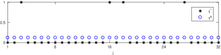
(a) $k=0$ (the initial point).

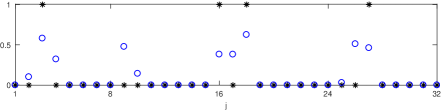
(b) $k=10$.

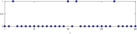
(c) $k=25$.

Figure 4: Entries in $t^{k}$ generated by PN-QP with $k=0,\ 10$, and $25$.

5.2 Comparison with Other Algorithms

In this subsection, we will compare the numerical performance of PN-QP for solving problem Eq. RSQP with different models and the corresponding algorithms, which are detailed below.

• Problem Eq. P solved by GPM [14]: GPM is essentially a gradient projection method whose projection step is taken directly over the discrete set $\mathcal{X}$. Due to its low computational complexity, it is able to solve the large-scale problem. Moreover, in our implementation, we modify its output by choosing the best point among all generated iterates (to improve its performance), instead of simply using the last iterate $x^{k}$ as the output.

• Problem Eq. P solved by SD [7]: SD is a typical tree search based method which searches for constellation points limited to a sphere with a predetermined radius centered on the vector of received signals $r$ to find the global solution. However, the complexity of SD is generally exponential, and hence it is impractical to solve the large-scale problem.

• Problem Eq. ERSDR1 solved by MOSEK [24]: There are several state-of-the-art solvers for SDRs including MOSEK and SDPNAL+ [28, 33, 36, 37]. Here we choose MOSEK since it is a classical interior-point algorithm based solver and is faster than SDPNAL+ for solving problem Eq. ERSDR1. As shown in Table 1, the size of problems Eq. ERSDR2 and Eq. ERSDR3 is significantly larger than that of problem Eq. ERSDR1, and the three problems are (mathematically) equivalent due to [15, Theorem 1] and the discussions in Section 3.3. Therefore, in our following tests, we do not compare the performance of solving problems Eq. ERSDR2 and Eq. ERSDR3. For $(t^{k},\,y^{k},\,Y^{k})$ of problem Eq. ERSDR1 returned by MOSEK, we perform the following rounding procedure to obtain a feasible point: project $(y^{k}_{j},\,y^{k}_{n+j})$ to $\mathcal{Y}$ in Eq. 6, and get $(y^{\star}_{j},\,y^{\star}_{n+j})$ by

  $$(y^{\star}_{j},\,y^{\star}_{n+j})\in\arg\underset{(u_{1},\,u_{2})\in\mathcal{Y}}{\min}\,(u_{1}-y^{k}_{j})^{2}+(u_{2}-y^{k}_{n+j})^{2},\ j=1,\ldots,n.$$

  Then return $x_{j}=y^{\star}_{j}+\mathrm{i}y^{\star}_{n+j}$, $j=1,\ldots,n$.

In our experiments, we set $M\in\{2,\,8,\,16\}$, $n\in\{16,\,32,\,64,\,128,\,256,\,512\}$, and $m=n$ or $m=2n$. We use the following two metrics to evaluate the performance of different algorithms: the symbol error rate (denoted by SER) [14, 31] as well as the running time in seconds (denoted by Time). More specifically, the SER is used to evaluate the detection error rate of different algorithms, which is calculated by

$$\frac{\text{The number of incorrectly recovered entries compared to }x^{*}}{\text{The length of transmitted signals }n}.$$

Time is used to evaluate the speed of different algorithms, which is particularly important for solving large-scale problems. We limit the maximum running time of each algorithm to be 3600 seconds. That is, we will terminate the algorithm if its running time is over $3600$ seconds and we use “—” to denote such case. The reported results below are obtained by averaging over 100 randomly generated instances.

Initial Points. Since both PN-QP and GPM require the initial points, we first compare the effects of different initial points on the detection results of the two algorithms. We test three initial points: the zero vector 0, the vector $t_{\boldsymbol{e}}$ defined as in Eq. 32, and the approximate solution $t_{ml}$ obtained by the minimum mean square error (MMSE) detector [14]. We report the results in Table 2, where for each setting $(m,\,n,\,M,\,\text{SNR})$ and each method, the winner is marked in bold among three initial points.

Table 2: Comparison of initial points for PN-QP and GPM.

$(m,\,n,\,M)$		Time(s)						SER($\%$)
	SNR	PN-QP			GPM			PN-QP			GPM
	(dB)	Eq. RSQP			Eq. P			Eq. RSQP			Eq. P
		0	$t_{\boldsymbol{e}}$	$t_{ml}$	0	$t_{\boldsymbol{e}}$	$t_{ml}$	0	$t_{\boldsymbol{e}}$	$t_{ml}$	0	$t_{\boldsymbol{e}}$	$t_{ml}$
$(64,\,32,\,8)$	24	0.034	0.034	0.012	0.001	0.001	0.000	0.00	0.00	0.00	12.44	12.31	0.00
	20	0.029	0.033	0.011	0.001	0.001	0.000	0.00	0.00	0.00	12.13	13.13	0.00
	16	0.030	0.036	0.011	0.001	0.001	0.000	0.00	0.00	0.00	7.06	9.16	0.00
	12	0.035	0.038	0.012	0.001	0.001	0.000	0.25	0.25	0.25	5.72	5.47	0.91
$(32,\,32,\,8)$	24	0.046	0.050	0.014	0.001	0.001	0.000	0.19	0.00	0.00	56.22	58.28	1.25
	20	0.045	0.048	0.017	0.001	0.001	0.000	1.06	0.25	0.25	57.50	57.19	2.78
	16	0.058	0.052	0.023	0.001	0.001	0.001	3.59	2.00	4.25	57.63	55.75	11.09
	12	0.063	0.063	0.031	0.001	0.001	0.001	17.59	16.13	20.28	52.13	52.16	25.44
$(64,\,32,\,16)$	24	0.079	0.091	0.027	0.001	0.001	0.000	0.00	0.00	0.00	40.75	40.41	0.00
	20	0.082	0.095	0.028	0.001	0.001	0.000	0.00	0.00	0.00	30.06	30.72	0.06
	16	0.096	0.115	0.036	0.001	0.001	0.000	2.63	2.31	2.78	32.06	29.94	3.22
	12	0.114	0.123	0.057	0.001	0.001	0.001	18.13	17.94	18.88	28.16	29.91	18.84
$(32,\,32,\,16)$	24	0.133	0.142	0.095	0.002	0.001	0.000	1.44	0.53	5.28	67.28	66.00	15.91
	20	0.171	0.176	0.133	0.002	0.001	0.000	6.75	5.19	13.09	68.53	69.34	22.03
	16	0.190	0.196	0.172	0.002	0.001	0.001	26.91	25.41	32.41	72.69	71.69	38.63
	12	0.198	0.203	0.158	0.001	0.001	0.001	48.34	46.53	48.84	68.91	69.53	52.56
$(1024,\,512,\,8)$	24	0.746	0.653	0.245	1.623	1.802	0.136	0.00	0.00	0.00	14.38	15.52	0.00
	20	0.767	0.676	0.240	0.891	1.175	0.134	0.00	0.00	0.00	5.82	9.28	0.00
	16	0.837	0.748	0.259	0.543	0.523	0.145	0.00	0.00	0.00	1.86	2.28	0.00
	12	1.153	1.053	0.583	0.351	0.351	0.201	0.26	0.25	0.27	0.42	0.40	0.38
$(512,\,512,\,8)$	24	1.235	1.108	0.461	1.519	1.471	0.116	0.00	0.00	0.00	57.48	57.74	0.00
	20	1.317	1.190	0.723	1.525	1.492	0.141	0.00	0.00	0.00	57.78	58.20	0.00
	16	1.810	1.621	1.676	1.555	1.430	0.923	0.10	0.10	0.10	58.14	58.38	8.55
	12	3.101	3.155	3.520	1.514	1.470	0.733	17.41	17.00	20.69	58.51	59.03	24.07
$(1024,\,512,\,16)$	24	1.469	1.431	0.512	3.646	3.900	0.136	0.00	0.00	0.00	55.38	55.37	0.00
	20	1.714	1.664	0.651	3.815	3.948	0.168	0.01	0.01	0.01	53.86	54.08	0.01
	16	2.616	2.492	1.852	4.094	3.983	0.295	1.92	1.95	2.11	47.75	48.16	2.04
	12	4.082	3.896	4.412	1.394	1.430	0.407	18.64	18.64	19.69	25.36	25.53	19.82
$(512,\,512,\,16)$	24	3.403	3.116	3.193	2.311	2.401	2.243	0.00	0.00	0.00	77.61	77.68	23.54
	20	7.071	6.434	8.134	2.426	2.450	2.235	3.13	3.13	8.98	77.97	77.97	33.35
	16	6.525	6.355	7.881	2.337	2.586	2.270	29.20	29.18	32.58	77.72	77.69	45.58
	12	6.900	6.686	8.725	2.326	2.199	2.360	48.27	48.14	50.17	78.29	78.13	55.01

It can be observed from Table 2 that in terms of the time for PN-QP, for small scale of $(m,\,n)$, $t_{ml}$ takes the smallest time whereas for large scale of $(m,\,n)$, $t_{\boldsymbol{e}}$ and $t_{ml}$ are comparable. Coming to the SER for PN-QP, $t_{\boldsymbol{e}}$ is more favorable among the three choices. In comparison, the SER by GPM varies quite a lot among the three choices of the initial point, and $t_{ml}$ is definitely the best initial point for GPM which will lead to a much smaller SER. In terms of the running time, it seems that $t_{ml}$ for PN-QP is preferable for small-scale problems whereas $t_{\boldsymbol{e}}$ leads to the smallest running time for PN-QP among the three choices when the size of problem $n$ is large (i.e., $n=512$). For GPM, $t_{ml}$ is also the winner from the perspective of running time. Based on the above observations, in our following test, we choose $t_{\boldsymbol{e}}$ as the initial point for PN-QP and the MMSE estimator $t_{ml}$ as the initial point for GPM. Here we would like to highlight that the numerical results with $n\geqslant 128$ which we show in this paper have not appeared in literature.

Results on Problems with $M\leqslant 8$. Next, we compare the performance of the four algorithms in the cases that $M=2$ and $M=8$. We also report the no interference lower bound (LB) results. This approach solves the MIMO detection problem with respect to each component $x_{j}$ assuming all the others being fixed to be the true transmitted signals. Again, the SER is obtained by dividing the total number of incorrectly estimated elements over the length of transmitted signals. The solution returned by LB can be viewed as the best possible result that the MIMO detection problem can be solved theoretically. Therefore, the above no interference LB can be used as the theoretical (and generally unachievable especially in the low SNR scenarios) lower bound of the SER of all the other approaches.

It can be observed from Table 3 and Table 4 that as the SNR decreases, the SER achieved by each algorithm increases, implying that the problem becomes more difficult. As shown in Table 3, when $M=2$, all methods perform well in terms of the SER.

From Table 3 and Table 4, one can see that the running time for SD becomes longer and even prohibitively high as the SNR decreases/$n$ increases, despite that SD provides the best SER among the four algorithms. For the other three algorithms, in general PN-QP provides the best SER, and MOSEK performs better than GPM in terms of the SER. For example, for $(m,\,n,\,M)=(128,\,128,\,8)$ and ${\rm SNR}=14$ dB, PN-QP takes $0.277$ seconds to return a solution with ${\rm SER}=4.57\%$, whereas MOSEK takes about one second to return a solution with a larger SER $7.14\%$, and GPM returns a solution with the SER being $17.13\%$ instantly (i.e., $0.012$ seconds). For such example, SD fails to return a solution within one hour. For the running time, GPM for solving problem Eq. P is the fastest one since it only involves gradient calculation and projection onto a discrete set. PN-QP for solving problem Eq. RSQP is fairly fast and its running time increases slowly as $n$ increases. This is due to the vector formulation of problem Eq. RSQP. MOSEK for solving problem Eq. ERSDR1 is not as fast as GPM and PN-QP. As $n$ increases, the running time increases much faster than that for PN-QP. Comparing $(m,\,n,\,M)=(256,\,256,\,8)$ with $(m,\,n,\,M)=(512,\,512,\,8)$, it can be observed that as $n$ increases from $256$ to $512$, the running time for MOSEK increases from about $10$ seconds to about $85$ seconds. This can be explained by the numbers of the variables (one $2n\times 2n$ matrix variable and one $2n+nM$ vector variable) and constraints (one $4n\times 4n$ positive semidefinite constraint, $6n$ equality constraints, and $nM$ inequality constraints) in Table 1. Therefore, in our subsequent test, we will not include SD and MOSEK.

To better understand the detection performance of the four algorithms, we plot Fig. 5, showing the SER with respect to the SNR for each algorithm. It can be seen from Fig. 5 that for $(m,\,n,\,M)=(16,\,16,\,8)$, SD performs the best since its SER curve coincides with the LB when the SNR is large. MOSEK also performs very well since the curve of MOSEK becomes parallel to the LB, i.e., a constant SER gap. However, this is not the case for PN-QP and GPM. For $(m,\,n,\,M)=(32,\,16,\,8)$, PN-QP, MOSEK, and SD are competitive, whereas SD is the best one.

Table 3: Time and SER comparison of PN-QP, MOSEK, GPM, and SD for solving MIMO detection problems with $M=2$.

$(m,\,n,\,M)$	SNR	Time(s)				SER($\%$)
		PN-QP	MOSEK	GPM	SD	PN-QP	MOSEK	GPM	SD	LB
	(dB)	Eq. RSQP	Eq. ERSDR1	Eq. P	Eq. P	Eq. RSQP	Eq. ERSDR1	Eq. P	Eq. P
$(32,\,32,\,2)$	22	0.004	0.338	0.001	0.003	0.00	0.00	0.00	0.00	0.00
	20	0.004	0.329	0.001	0.003	0.00	0.00	0.00	0.00	0.00
	18	0.004	0.335	0.001	0.005	0.00	0.00	0.00	0.00	0.00
	16	0.005	0.338	0.001	0.012	0.00	0.00	0.00	0.00	0.00
	14	0.004	0.348	0.001	0.047	0.00	0.00	0.03	0.00	0.00
	12	0.004	0.369	0.001	0.110	0.00	0.00	0.16	0.00	0.00
$(64,\,64,\,2)$	22	0.008	0.456	0.001	0.007	0.00	0.00	0.00	0.00	0.00
	20	0.008	0.460	0.001	0.013	0.00	0.00	0.00	0.00	0.00
	18	0.008	0.469	0.001	0.035	0.00	0.00	0.00	0.00	0.00
	16	0.008	0.503	0.001	0.158	0.00	0.00	0.00	0.00	0.00
	14	0.008	0.534	0.001	1.392	0.00	0.00	0.00	0.00	0.00
	12	0.008	0.607	0.001	10.251	0.00	0.00	0.09	0.00	0.00
$(128,\,128,\,2)$	22	0.025	1.256	0.003	0.815	0.00	0.00	0.00	0.00	0.00
	20	0.025	1.319	0.003	12.260	0.00	0.00	0.00	0.00	0.00
	18	0.026	1.500	0.003	284.234	0.00	0.00	0.00	0.00	0.00
	16	0.030	1.723	0.004	2348.488	0.00	0.00	0.00	0.00	0.00
	14	0.030	1.783	0.004	—	0.00	0.00	0.00	—	0.00
	12	0.027	2.158	0.003	—	0.00	0.00	0.02	—	0.00
$(256,\,256,\,2)$	22	0.111	7.249	0.013	—	0.00	0.00	0.00	—	0.00
	20	0.112	7.408	0.013	—	0.00	0.00	0.00	—	0.00
	18	0.113	7.683	0.014	—	0.00	0.00	0.00	—	0.00
	16	0.115	8.502	0.014	—	0.00	0.00	0.00	—	0.00
	14	0.114	12.064	0.014	—	0.00	0.00	0.00	—	0.00
	12	0.117	15.292	0.015	—	0.00	0.00	0.01	—	0.00
$(512,\,512,\,2)$	22	0.198	58.730	0.092	—	0.00	0.00	0.00	—	0.00
	20	0.200	61.319	0.092	—	0.00	0.00	0.00	—	0.00
	18	0.201	64.035	0.092	—	0.00	0.00	0.00	—	0.00
	16	0.207	71.433	0.097	—	0.00	0.00	0.00	—	0.00
	14	0.216	113.457	0.106	—	0.00	0.00	0.00	—	0.00
	12	0.230	135.229	0.110	—	0.00	0.00	0.00	—	0.00

Table 4: Time and SER comparison of PN-QP, MOSEK, GPM, and SD for solving MIMO detection problems with $M=8$.

$(m,\,n,\,M)$	SNR	Time(s)				SER($\%$)
		PN-QP	MOSEK	GPM	SD	PN-QP	MOSEK	GPM	SD	LB
	(dB)	Eq. RSQP	Eq. ERSDR1	Eq. P	Eq. P	Eq. RSQP	Eq. ERSDR1	Eq. P	Eq. P
$(32,\,32,\,8)$	22	0.044	0.362	0.001	0.208	0.00	0.00	1.31	0.00	0.00
	20	0.050	0.307	0.001	1.666	0.00	0.13	2.13	0.00	0.00
	18	0.051	0.340	0.001	19.923	0.00	0.25	4.06	0.00	0.00
	16	0.051	0.335	0.001	305.642	1.63	1.94	9.59	0.09	0.03
	14	0.060	0.403	0.002	2495.598	3.13	6.88	21.88	3.13	0.00
	12	0.067	0.351	0.001	—	13.94	14.81	23.47	—	3.69
$(64,\,64,\,8)$	22	0.126	0.513	0.002	769.366	0.00	0.00	0.22	0.00	0.00
	20	0.134	0.537	0.002	—	0.00	0.00	0.06	—	0.00
	18	0.132	0.507	0.003	—	0.00	0.39	3.09	—	0.00
	16	0.137	0.519	0.002	—	0.78	1.84	7.94	—	0.02
	14	0.150	0.510	0.003	—	5.92	7.28	15.53	—	0.66
	12	0.188	0.506	0.002	—	16.34	16.44	24.97	—	3.38
$(128,\,128,\,8)$	22	0.156	1.763	0.004	—	0.00	0.00	0.11	—	0.00
	20	0.164	1.730	0.005	—	0.00	0.00	0.95	—	0.00
	18	0.172	1.701	0.006	—	0.01	0.24	2.64	—	0.01
	16	0.189	1.675	0.010	—	0.38	1.88	6.73	—	0.06
	14	0.277	1.651	0.012	—	4.57	7.14	17.13	—	0.63
	12	0.307	1.555	0.008	—	15.89	15.47	23.63	—	3.27
$(256,\,256,\,8)$	22	0.342	10.558	0.018	—	0.00	0.00	0.00	—	0.00
	20	0.353	10.290	0.029	—	0.00	0.02	0.98	—	0.00
	18	0.379	10.153	0.041	—	0.00	0.32	2.02	—	0.00
	16	0.450	10.144	0.076	—	0.08	2.08	7.54	—	0.05
	14	0.587	9.799	0.097	—	4.11	7.45	15.85	—	0.75
	12	0.660	9.748	0.067	—	16.60	16.25	23.22	—	3.18
$(512,\,512,\,8)$	22	1.193	88.809	0.134	—	0.00	0.00	0.00	—	0.00
	20	1.303	91.365	0.177	—	0.00	0.01	0.09	—	0.00
	18	1.436	90.253	0.297	—	0.00	0.25	0.88	—	0.00
	16	1.825	88.638	0.929	—	0.08	2.23	6.68	—	0.06
	14	3.177	86.758	1.455	—	2.46	7.29	16.82	—	0.66
	12	3.482	85.408	0.765	—	16.41	16.15	22.97	—	3.17

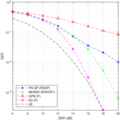
(a) $(m,\,n,\,M)=(16,\,16,\,8)$.

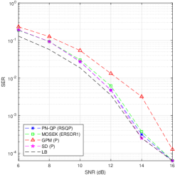
(b) $(m,\,n,\,M)=(32,\,16,\,8)$.

Figure 5: The SER performance of the four algorithms under different SNRs.

Results on Problems with $M\geqslant 8$. We further compare the performance of PN-QP and GPM on $M=16$. According to Table 5, as the SNR decreases, PN-QP provides a lower SER than GPM, implying that PN-QP achieves better detection performance. For instance, for $(m,\,n,\,M)=(512,\,512,\,16)$ with ${\rm SNR}=20$ dB, PN-QP returns a solution with ${\rm SER}=3.46\%$, whereas the SER of GPM is $33.67\%$. We also present more comparisons of the two algorithms in Fig. 6. It can be observed from Fig. 6 that as the SNR increases, the SER curve of PN-QP tends to coincide with the LB. In contrast, there is a large gap between the SER curve of GPM with the LB, especially in the case where $m=n$.

Table 5: Time and SER comparison of PN-QP and GPM for solving MIMO detection problems with $M=16$.

$(m,\,n,\,M)$	SNR	Time(s)		SER($\%$)
		PN-QP	GPM	PN-QP	GPM	LB
	(dB)	Eq. RSQP	Eq. P	Eq. RSQP	Eq. P
$(256,\,128,\,16)$	30	0.203	0.005	0.00	0.00	0.00
	25	0.210	0.004	0.00	0.00	0.00
	20	0.235	0.004	0.02	0.02	0.01
	15	0.395	0.007	4.49	5.23	2.66
$(128,\,128,\,16)$	30	0.386	0.007	0.00	2.81	0.00
	25	0.406	0.018	0.00	17.41	0.00
	20	0.549	0.023	8.42	34.49	0.74
	15	0.572	0.023	33.09	46.80	12.58
$(512,\,256,\,16)$	30	0.432	0.023	0.00	0.00	0.00
	25	0.466	0.024	0.00	0.00	0.00
	20	0.518	0.026	0.02	0.02	0.01
	15	0.774	0.046	4.27	4.61	2.80
$(256,\,256,\,16)$	30	0.862	0.047	0.00	1.60	0.00
	25	0.986	0.179	0.00	18.45	0.00
	20	1.513	0.186	4.80	34.61	0.65
	15	1.603	0.190	34.89	48.95	11.55
$(1024,\,512,\,16)$	30	1.355	0.156	0.00	0.00	0.00
	25	1.416	0.155	0.00	0.00	0.00
	20	1.722	0.191	0.01	0.01	0.01
	15	3.273	0.397	4.48	4.76	2.85
$(512,\,512,\,16)$	30	2.640	0.380	0.00	1.28	0.00
	25	2.980	2.298	0.00	19.43	0.00
	20	6.337	2.337	3.46	33.67	0.59
	15	6.718	2.390	33.88	48.36	12.09

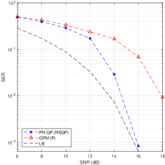
(a) $(m,\,n,\,M)=(512,\,512,\,8)$.

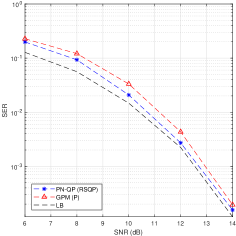
(b) $(m,\,n,\,M)=(1024,\,512,\,8)$.

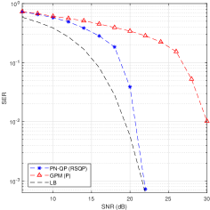
(c) $(m,\,n,\,M)=(512,\,512,\,16)$.

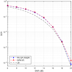
(d) $(m,\,n,\,M)=(1024,\,512,\,16)$.

Figure 6: The SER performance of PN-QP and GPM under different SNRs.

Based on the above comparisons, our proposed algorithm for solving the MIMO detection problem is more efficient than existing algorithms for solving large-scale problems. Specifically, compared to MOSEK and SD, PN-QP is more efficient; compared to GPM, PN-QP achieves better detection performance. To conclude, PN-QP is demonstrated to be a competitive candidate for solving the large-scale MIMO detection problem.

6 Conclusions

In this paper, we proposed an efficient algorithm called PN-QP for solving the large-scale MIMO detection problem, motivated by the massive MIMO technology. The proposed algorithm is essentially a quadratic penalty method applied to solve an SQP relaxation, i.e., problem Eq. RSQP, of the original problem. Two key features of the proposed algorithm, which make it particularly suitable to solve the large-scale problems, are: (i) it is based on the relaxation problem Eq. RSQP, whose numbers of variables and constraints are significantly less than those of the SDRs; and (ii) our proposed algorithm is custom-designed to identify the support set of the optimal solution by judiciously exploiting the special structure of the problem, instead of finding the solution itself, which thus substantially reduces the computational complexity of the proposed algorithm. The above two reasons lead to the better numerical performance of the proposed algorithm. In particular, our extensive simulation results show that our proposed algorithm compares favorably with the state-of-the-art algorithms (including SD and SDR based approaches) for solving the MIMO detection problem. When applied to solve large-scale problems, our proposed algorithm achieves significantly better detection performance than GPM.

Appendix A Proof of Theorem 2.3

We need the following results to prove Theorem 2.3.

Proposition A.1.

Let $Q$, $\widehat{Q}$, and $G$ be defined in Eq. 3, Eq. 7, and Eq. 11, respectively. We have

• $q_{jj}=\sum_{k=1}^{m}|h_{kj}|^{2}$ for $j=1,\ldots,n$;

• $\hat{q}_{kj}=\hat{q}_{jk}=\hat{q}_{(n+j)(n+k)}=\hat{q}_{(n+k)(n+j)}$, $\hat{q}_{(n+j)k}=\hat{q}_{k(n+j)}=-\hat{q}_{(n+k)j}=-\hat{q}_{j(n+k)}$, $\hat{q}_{jj}=\hat{q}_{(n+j)(n+j)}=q_{jj}$, and $\hat{q}_{(n+j)j}=\hat{q}_{j(n+j)}=0$ for $j,\ k=1,\ldots,n$;

• $S_{jk}=\hat{q}_{jk}\alpha\alpha^{\top}+\hat{q}_{(n+j)k}\beta\alpha^{\top}+\hat{q}_{j(n+k)}\alpha\beta^{\top}+\hat{q}_{(n+j)(n+k)}\beta\beta^{\top}$ and $S_{jk}=S_{kj}^{\top}$ for $j,\ k=1,\ldots,n$; and

• ${\rm diag}(S_{jj})=q_{jj}\boldsymbol{e}$ for $j=1,\ldots,n$.

Proof A.2.

(i) By the definition of $Q$ in Eq. 3, there is

$$q_{jj}=\sum_{k=1}^{m}h_{kj}^{\dagger}h_{kj}=\sum_{k=1}^{m}|h_{kj}|^{2},$$

which gives (i).

(ii) By the definitions of $\widehat{Q}$ in Eq. 7 and $Q$ in Eq. 3, the first three results in (ii) hold naturally. Note that due to (i), there is ${\rm diag}({\rm Im}(Q))=\textbf{0},$ implying the fourth result in (ii).

(iii) Let $P$ have the partition as $P=\begin{bmatrix}P_{1}&\cdots&P_{n}\end{bmatrix}$, where $P_{j}\in\mathbb{R}^{2n\times M}$ takes the following form:

(33) $$\begin{array}[]{ccccccccccc}P_{j}^{\top}=[\textbf{0}&\cdots&\textbf{0}&\alpha&\textbf{0}&\cdots&\textbf{0}&\beta&\textbf{0}&\cdots&\textbf{0}]^{\top}.\\ &&&\uparrow&&&&\uparrow&&&\\ &\lx@intercol\hfil\text{\footnotesize{the $j$-th block}}\lx@intercol&\lx@intercol\hfil\text{\footnotesize{the $(n+j)$-th block}}\hfil\lx@intercol&\end{array}$$

By the definition and partition of $G$ in Eqs. 11 and 13, we have

$$G =P^{\top}\widehat{Q}P=\begin{bmatrix}P_{1}&\cdots&P_{n}\end{bmatrix}^{\top}\widehat{Q}\begin{bmatrix}P_{1}&\cdots&P_{n}\end{bmatrix}$$

$$=\begin{bmatrix}P_{1}^{\top}\widehat{Q}P_{1}&\cdots&P_{1}^{\top}\widehat{Q}P_{n}\\ \vdots&\ddots&\vdots\\ P_{n}^{\top}\widehat{Q}P_{1}&\cdots&P_{n}^{\top}\widehat{Q}P_{n}\end{bmatrix}=\begin{bmatrix}S_{11}&\cdots&S_{1n}\\ \vdots&\ddots&\vdots\\ S_{n1}&\cdots&S_{nn}\end{bmatrix},$$

which, together with Eqs. 33 and 7, further implies

$$S_{jk} =P_{j}^{\top}\widehat{Q}P_{k}$$

$$=\begin{bmatrix}\hat{q}_{j1}\alpha+\hat{q}_{(n+j)1}\beta&\cdots&\hat{q}_{j(2n)}\alpha+\hat{q}_{(n+j)(2n)}\beta\end{bmatrix}P_{k}$$

$$=\hat{q}_{jk}\alpha\alpha^{\top}+\hat{q}_{(n+j)k}\beta\alpha^{\top}+\hat{q}_{j(n+k)}\alpha\beta^{\top}+\hat{q}_{(n+j)(n+k)}\beta\beta^{\top}.$$

The proof of the first result in (iii) is finished. With the first result in (iii), as well as the first two results in (ii), there is

$$S_{jk} =\hat{q}_{jk}\alpha\alpha^{\top}+\hat{q}_{(n+j)k}\beta\alpha^{\top}+\hat{q}_{j(n+k)}\alpha\beta^{\top}+\hat{q}_{(n+j)(n+k)}\beta\beta^{\top}$$

$$=\hat{q}_{kj}\alpha\alpha^{\top}+\hat{q}_{k(n+j)}\beta\alpha^{\top}+\hat{q}_{(n+k)j}\alpha\beta^{\top}+\hat{q}_{(n+k)(n+j)}\beta\beta^{\top}$$

$$=(\hat{q}_{kj}\alpha\alpha^{\top}+\hat{q}_{k(n+j)}\alpha\beta^{\top}+\hat{q}_{(n+k)j}\beta\alpha^{\top}+\hat{q}_{(n+k)(n+j)}\beta\beta^{\top})^{\top}$$

$$=S_{kj}^{\top}.$$

We get the second result in (iii).

(iv) Due to (iii), there is

$$S_{jj} =\hat{q}_{jj}\alpha\alpha^{\top}+\hat{q}_{(n+j)j}\beta\alpha^{\top}+\hat{q}_{j(n+j)}\alpha\beta^{\top}+\hat{q}_{(n+j)(n+j)}\beta\beta^{\top}$$

$$=q_{jj}(\alpha\alpha^{\top}+\beta\beta^{\top}).$$

Recall the definitions of $\alpha$, $\beta$ in Eq. 9 and $\theta_{k}$ in Eq. 6. The $k$-th diagonal entry of $S_{jj}$ takes the following form:

$$q_{jj}(\cos^{2}\left(\theta_{k}\right)+\sin^{2}\left(\theta_{k}\right))=q_{jj},\ k=1,\ldots,M.$$

Therefore, ${\rm diag}(S_{jj})=q_{jj}\boldsymbol{e}$. The proof is finished.

Proposition A.3.

Under the constraints in problem Eq. SQP2, there is

(34) $$\sum_{j=1}^{n}\bar{t}_{j}^{\top}S_{jj}\bar{t}_{j}=\|H\|_{2}^{2}.$$

Proof A.4.

Under the constraints in problem Eq. SQP2, for each $\bar{t}_{j}$, there exists $l_{j}\in\{1,\ldots,M\}$, such that $\bar{t}_{j}=e_{l_{j}}$, where $e_{l_{j}}$ denotes the $l_{j}$-th column in the identity matrix $I\in\mathbb{R}^{M\times M}$. As a result, with (i) and (iv) in Proposition A.1, there is

$$\sum_{j=1}^{n}\bar{t}_{j}^{\top}S_{jj}\bar{t}_{j}=\sum_{j=1}^{n}e_{l_{j}}^{\top}S_{jj}e_{l_{j}}=\sum_{j=1}^{n}q_{jj}=\sum_{j=1}^{n}\sum_{k=1}^{m}|h_{kj}|^{2}=\|H\|_{2}^{2},$$

which gives Eq. 34. The proof is finished.

Now we are ready to prove Theorem 2.3.

Proof A.5.

Using Proposition A.3, we have

$$h(t)-f(t)=\sum_{j=1}^{n}\bar{t}_{j}^{\top}S_{jj}\bar{t}_{j}=\|H\|_{2}^{2}.$$

This, together with the fact that the constraints of problems Eq. SQP1 and Eq. SQP2 are the same, implies that problems Eq. SQP1 and Eq. SQP2 are equivalent.

References

- [1] M. A. Albreem, M. Juntti, and S. Shahabuddin, Massive MIMO detection techniques: A survey, IEEE Communications Surveys and Tutorials, 21 (2019), pp. 3109–3132.
- [2] D. P. Bertsekas, Projected Newton methods for optimization problems with simple constraints, SIAM Journal on Control and Optimization, 20 (1982), pp. 221–246.
- [3] S. A. Busari, K. M. S. Huq, S. Mumtaz, L. Dai, and J. Rodriguez, Millimeter-wave massive MIMO communication for future wireless systems: A survey, IEEE Communications Surveys and Tutorials, 20 (2018), pp. 836–869.
- [4] A. M. Chan and I. Lee, A new reduced-complexity sphere decoder for multiple antenna systems, in Proceedings of IEEE International Conference on Communications, New York, 2002, pp. 460–464.
- [5] Cisco, Cisco visual networking index: Global mobile data traffic forecast update, 2017–2022, 2019, https://www.cisco.com/c/en/us/solutions/collateral/service-provider/visual-networking-index-vni/white-paper-c11-738429.html (accessed 2019-12-10).
- [6] C. Cui, Q.-N. Li, L. Qi, and H. Yan, A quadratic penalty method for hypergraph matching, Journal of Global Optimization, 70 (2018), pp. 237–259.
- [7] O. Damen, A. Chkeif, and J.-C. Belfiore, Lattice code decoder for space-time codes, IEEE Communications Letters, 4 (2000), pp. 161–163.
- [8] J. Jaldén, Detection for multiple input multiple output channels, PhD thesis, KTH Royal Institute of Technology, 2006.
- [9] J. Jaldén and B. Ottersten, On the complexity of sphere decoding in digital communications, IEEE Transactions on Signal Processing, 53 (2005), pp. 1474–1484.
- [10] J. Jaldén, D. Seethaler, and G. Matz, Worst- and average-case complexity of LLL lattice reduction in MIMO wireless systems, in Proceedings of IEEE International Conference on Acoustics, Speech and Signal Processing, Las Vegas, 2008, pp. 2685–2688.
- [11] R. Jiang, Y.-F. Liu, C. Bao, and B. Jiang, Tightness and equivalence of semidefinite relaxations for MIMO detection, 2021, https://arxiv.org/abs/2102.04586.
- [12] A. K. Lenstra, H. W. Lenstra, and L. Lovász, Factoring polynomials with rational coefficients, Mathematische Annalen, 261 (1982), pp. 515–534.
- [13] Q.-N. Li and D.-H. Li, A projected semismooth Newton method for problems of calibrating least squares covariance matrix, Operations Research Letters, 39 (2011), pp. 103–108.
- [14] H. Liu, M.-C. Yue, A. M.-C. So, and W.-K. Ma, A discrete first-order method for large-scale MIMO detection with provable guarantees, in Proceedings of IEEE Workshop on Signal Processing Advances in Wireless Communications, Sapporo, 2017, pp. 669–673.
- [15] Y.-F. Liu, Z. Xu, and C. Lu, On the equivalence of semidifinite relaxations for MIMO detection with general constellations, in Proceedings of IEEE International Conference on Acoustics, Speech, and Signal Processing, Brighton, 2019, pp. 4549–4553.
- [16] M. P. Lotter and P. V. Rooyen, Space division multiple access for cellular CDMA, in Proceedings of IEEE International Symposium on Spread Spectrum Techniques and Applications, Sun City, 1998, pp. 959–964.
- [17] C. Lu, Y.-F. Liu, W.-Q. Zhang, and S. Zhang, Tightness of a new and enhanced semidefinite relaxation for MIMO detection, SIAM Journal on Optimization, 29 (2019), pp. 719–742.
- [18] C. Lu, Y.-F. Liu, and J. Zhou, An efficient global algorithm for nonconvex complex quadratic problems with applications in wireless communications, in Proceedings of IEEE/CIC International Conference on Communications in China, Qingdao, 2017, pp. 1–5.
- [19] C. Lu, Y.-F. Liu, and J. Zhou, An enhanced SDR based global algorithm for nonconvex complex quadratic programs with signal processing applications, IEEE Open Journal of Signal Processing, 1 (2020), pp. 120–134.
- [20] Z.-Q. Luo, X. Luo, and M. Kisialiou, An efficient quasi-maximum likelihood decoder for PSK signals, in Proceedings of IEEE International Conference on Acoustics, Speech, and Signal Processing, Hong Kong, 2003, pp. 561–564.
- [21] W.-K. Ma, P.-C. Ching, and Z. Ding, Semidefinite relaxation based multiuser detection for M-ary PSK multiuser systems, IEEE Transactions on Signal Processing, 52 (2004), pp. 2862–2872.
- [22] A. Mobasher, M. Taherzadeh, R. Sotirov, and A. K. Khandani, A near-maximum-likelihood decoding algorithm for MIMO systems based on semi-definite programming, IEEE Transactions on Information Theory, 53 (2007), pp. 3869–3886.
- [23] A. F. Molisch, V. V. Ratnam, S. Han, Z. Li, S. L. H. Nguyen, L. Li, and K. Haneda, Hybrid beamforming for massive MIMO: A survey, IEEE Communications Magazine, 55 (2017), pp. 134–141.
- [24] MOSEK ApS, MOSEK optimization toolbox for MATLAB Release 9.2.29, 2020, https://docs.mosek.com/9.2/toolbox.pdf.
- [25] J. Nocedal and S. Wright, Numerical Optimization, Springer-Verlag, New York, 2006.
- [26] M. Pohst, On the computation of lattice vectors of minimal length, successive minima and reduced bases with applications, ACM Sigsam Bulletin, 15 (1981), pp. 37–44.
- [27] A. M.-C. So, Probabilistic analysis of the semidefinite relaxation detector in digital communications, in Proceedings of the Twenty-First Annual ACM-SIAM Symposium on Discrete Algorithms, Austin, 2010, pp. 698–711.
- [28] D. Sun, K.-C. Toh, Y. Yuan, and X.-Y. Zhao, SDPNAL+: A MATLAB software for semidefinite programming with bound constraints (version 1.0), Optimization Methods and Software, 35 (2020), pp. 87–115.
- [29] P. H. Tan and L. K. Rasmussen, The application of semidefinite programming for detection in CDMA, IEEE Journal on Selected Areas in Communications, 19 (2001), pp. 1442–1449.
- [30] S. Verdú, Computational complexity of optimum multiuser detection, Algorithmica, 4 (1989), pp. 303–312.
- [31] H.-T. Wai, W.-K. Ma, and A. M.-C. So, Cheap semidefinite relaxation MIMO detection using row-by-row block coordinate descent, in Proceedings of IEEE International Conference on Acoustics, Speech and Signal Processing, Prague, 2011, pp. 3256–3259.
- [32] Z. Xie, C. K. Rushforth, R. T. Short, and T. K. Moon, Joint signal detection and parameter estimation in multiuser communications, IEEE Transactions on Communications, 41 (1993), pp. 1208–1216.
- [33] L. Yang, D. Sun, and K.-C. Toh, SDPNAL+: A majorized semismooth Newton-CG augmented Lagrangian method for semidefinite programming with nonnegative constraints, Mathematical Programming Computation, 7 (2015), pp. 331–366.
- [34] S. Yang and L. Hanzo, Fifty years of MIMO detection: The road to large-scale MIMOs, IEEE Communications Surveys and Tutorials, 17 (2015), pp. 1941–1988.
- [35] H. Yao, Efficient signal, code, and receiver designs for MIMO communication systems, PhD thesis, Massachusetts Institute of Technology, 2003.
- [36] X.-Y. Zhao, A semismooth Newton-CG augmented Lagrangian method for large scale linear and convex quadratic SDPs, PhD thesis, National University of Singapore, 2009.
- [37] X.-Y. Zhao, D. Sun, and K.-C. Toh, A Newton-CG augmented Lagrangian method for semidefinite programming, SIAM Journal on Optimization, 20 (2010), pp. 1737–1765.
- [38] Q. Zhou and X. Ma, Element-based lattice reduction algorithms for large MIMO detection, IEEE Journal on Selected Areas in Communications, 31 (2013), pp. 274–286.