P3GM: Private High-Dimensional Data Release via Privacy Preserving Phased Generative Model¹

Abstract

How can we release a massive volume of sensitive data while mitigating privacy risks? Privacy-preserving data synthesis enables the data holder to outsource analytical tasks to an untrusted third party. The state-of-the-art approach for this problem is to build a generative model under differential privacy, which offers a rigorous privacy guarantee. However, the existing method cannot adequately handle high dimensional data. In particular, when the input dataset contains a large number of features, the existing techniques require injecting a prohibitive amount of noise to satisfy differential privacy, which results in the outsourced data analysis meaningless. To address the above issue, this paper proposes privacy-preserving phased generative model (P3GM), which is a differentially private generative model for releasing such sensitive data. P3GM employs the two-phase learning process to make it robust against the noise, and to increase learning efficiency (e.g., easy to converge). We give theoretical analyses about the learning complexity and privacy loss in P3GM. We further experimentally evaluate our proposed method and demonstrate that P3GM significantly outperforms existing solutions. Compared with the state-of-the-art methods, our generated samples look fewer noises and closer to the original data in terms of data diversity. Besides, in several data mining tasks with synthesized data, our model outperforms the competitors in terms of accuracy.

I Introduction

The problem of private data release, including privacy-preserving data publishing (PPDP) [30] [40] and privacy-preserving data synthesis (PPDS) [5] [7] [25] [44], has become increasingly important in recent years. We often encounter situations where a data holder wishes to outsource analytical tasks to the data scientists in a third party, and even in a different division in the same office, without revealing private, sensitive information. This outsourced data analysis raises privacy issues that the details of the private datasets, such as information about the census, health data, and financial records, are revealed to an untrusted third-party. Due to the growth of data science and smart devices, high dimensional, complex data related to an individual, such as face images for authentications and daily location traces, have been collected. In each example, there are many potential usages, privacy risks, and adversaries.

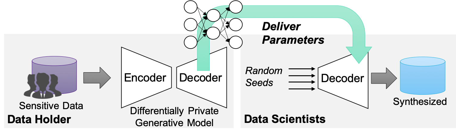
Figure 1: Privacy-preserving data synthesis via sharing a decoder of a differentially private generative model.

For the PPDP, a traditional approach is to ensure $k$-anonymity [40]. There are lots of anonymization algorithms for various data domains [4] [16] [30]. However, $k$-anonymity does not take into account adversaries’ background knowledge.

For releasing private statistical aggregates, differential privacy (DP in short) is known as the golden standard privacy notion [17]. Differential privacy seeks a rigorous privacy guarantee, without making restrictive assumptions about the adversary. Informally, this model requires that what can be learned from the released data is approximately the same, whether or not any particular individual was included in the input database. Differential privacy is used in broad domains and applications [7] [11] [36]. The importance of DP can be seen from the fact that US census announced ’2020 Census results will be protected using “differential privacy,” the new gold standard in data privacy protection’ [3] [9].

Differentially private data synthesis (DPDS) builds a generative model satisfying DP to produce privacy-preserving synthetic data from the sensitive data. It has been well-studied in the literature [5] [12] [25] [42] [44] [45]. DPDS protects privacy by sharing a differentially private generative model to the third party, instead of the raw datasets (Figure 1). In recent years, NIST held a competition in which contestants proposed a mechanism for DPDS while maintaining a dataset’s utility for analysis [35].

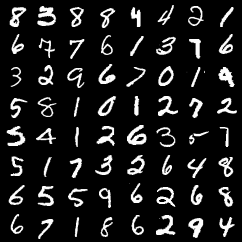
(a) MNIST (original)

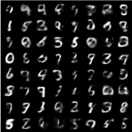
(b) VAE [27]

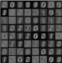
(c) DP-VAE (VAE w/ DP-SGD)

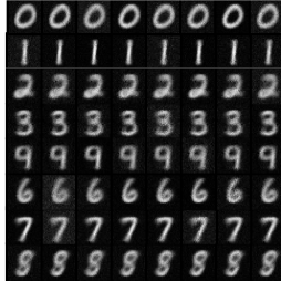
(d) DP-GM [5]

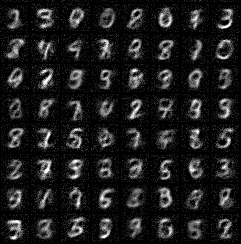
(e) Proposed Method

Figure 2: Sampled images from (b) VAE [27], (c) DP-VAE, (d) DP-GM [5] and (e) proposed method P3GM. These four models are trained with (a) MNIST. (b), (c) and (d) satisfies ($1,10^{-5}$)-differential privacy. Comparing the images sampled from DP-VAE and DP-GM, P3GM generates finer and more diverse samples. P3GM generates images that are visually closer to (a) and (b).

	PrivBayes [44]	Ryan’s [31]	VAE with DP-SGD	DP-GM [5]	P3GM (ours)
PPDS under differential privacy	✓	✓	✓	✓	✓
Utility in classification tasks	✓				✓
Capacity for high dimensional data		✓		✓	✓

TABLE I: Contrast with competitors. Only the proposed method achieves all requirements in PPDS for high dimensional data.

To preserve utility in data mining and machine learning tasks, a generative model should have the following properties: 1) data generated by the generative model follows actual data distribution; and 2) it can generate high dimensional data. However, the existing DPDS algorithms are insufficient for high dimensional data. When the input dataset contains a large number of features, the existing techniques require injecting a prohibitive amount of noise to satisfy DP. This issue results in the outsourced data analysis meaningless.

We now explain the existing models and their issues summarized in Table I. DPDS has been studied in the past ten years. Traditional approaches are based on capturing probabilistic models, low rank structure, and learning statistical characteristics from original sensitive database [12] [44] [45]. PrivBayes [44] is a generative model that constructs a Bayesian network with DP guarantee. However, since PrivBayes only constructs the Bayesian network among a few attributes, it is not suitable for high dimensional data. Ryan [31]was the winner of the NIST’s competition by outperforming PrivBayes. Ryan’s algorithm includes two steps to synthesize a dataset: 1) measures a chosen set of 1, 2, and 3-way marginals of the dataset with Gaussian mechanism, and 2) makes a dataset that has those marginals. We note that this algorithm requires public information to get the crucial set of 1, 2, and 3-way marginals.

Deep generative models have been significantly improved in the past few years. According to the advancement, constructing deep generative models under differential privacy is also a promising direction. We have two distinguished generative models: generative adversarial nets (GAN) [21] and variational autoencoder (VAE) [26] [27].

GANs can generate high quality data by optimizing a minimax objective. However, it is well known that samples from GANs do not fully capture the diversity of the true distribution due to mode collapse. Furthermore, GANs are challenging to evaluate, and require a lot of iterations to converge. Therefore, under differential privacy, such learning processes tend to inject a vast amount of noise. Actually, existing GAN based models with DP have significant limitations. DP-GAN [42] needs to construct a generative model for each digit on MNIST, to avoid the lack of diversity due to mode collapse. In [25], PATE-GAN demonstrated its effectiveness only for low-dimensional table data having tens of attributes.

In contrast, VAEs do not suffer from the problems of mode collapse and lack of diversity seen in GANs. However, recently proposed VAEs under DP constraints are not sufficient. A simple extension of VAE to satisfy DP is employing DP-SGD [2], which injects noise on stochastic gradients. However, it also produces noisy samples (see Figure 2c). It is due to that the learning process of VAE is also complicated. DP-GM [5] proposed a differentially private model based on VAE. DP-GM employs a simplified process that first partitions data by $k$-means clustering and then trains disjoint VAEs for each partition. As a result, DP-GM can craft samples with less noise, but these samples are close to the centroids of the clusters. This means DP-GM causes mode collapse accompanied by breaking the diversity of samples so that it can generate clear samples (see Figure 2d). In other words, the generated data does not follow the actual distribution of data, which causes low performance for data mining tasks. For example, DP-GM generates clear images in Figure 2d, but the accuracy of a classifier trained with the generated images results in $0.49$. In this paper, we study a differentially private generative model that generates diverse samples; the generated data follows the actual distribution.

I-A Our Contributions

In this paper, we propose a new generative model that satisfies DP, named privacy preserved phased generative model (P3GM). Using this model, we can publish the generated data in a way which meets the following requirements:

• Privacy of each data holder is protected with DP.

• The original data can be high dimensional.

• The generated data approximates the actual distribution of original data well enough to preserve utility for data mining tasks.

Because of the above properties, we can use P3GM for sharing a dataset with sensitive data to untrusted third-party such as a data scientist to analyze the data while preserving privacy.

The novelty of our paper is the new generative model with two-phased training. P3GM is based on VAE, which has an expressive power of various distributions for high dimensional data. However, P3GM has more tolerance to the noise for DP than VAE. Our training model is the encode-decoder model same as VAE, but the training procedure separates the VAE’s end-to-end training into two phases: training the encoder and training the decoder with the fixed encoder, which increases the robustness against the noise for DP. Training of the decoder becomes stable because of the fixed encoder. We define objective functions for each training to maximize the likelihood of our model. We show that if the optimal value is given in the training of the encoder, the decoder has the possibility to generate data that follows the actual distribution. Moreover, we theoretically describe why our two-phased training works better than end-to-end training under DP.

Furthermore, we give a realization of P3GM and a theoretical analysis of its privacy guarantee. To show that generated data preserve utility for data mining tasks, we conduct classification tasks using data generated by the above example with real-world datasets. Our model outperforms state-of-the-art techniques [5, 44] concerning the performances of the classifications under the same privacy protection level.

I-B Preview of Results

Figure 2 shows generated samples from (b) VAE [27], (c) VAE [27] with DP-SGD [2] (we call DP-VAE), (d) DP-GM [5], and (e) our proposed method P3GM. All methods are trained from (a) the MNIST dataset, and (c), (d) and (e) satisfy ($1,10^{-5}$)-DP. Behind the non-private method (b), samples from DP-VAE (c) look very noisy. Samples from DP-GM (d) are very fine, but it generates less diverse samples for each digit. Our proposed method (e) shows less noise and well diverse samples than (c) and (d). P3GM can generate images that are visually close to original data (a) and samples from the non-private model (b). Detailed empirical evaluations with several data mining tasks are provided in the latter part of this paper.

I-C Related Works

For releasing private statistical aggregates of curated database, differential privacy is used for privatization mechanisms. Traditionally, releasing count data (i.e., histograms) has been studied very well [14] [29] [43].To release statistical outputs described by complex queries, several works addressed differentially private indexing [39] and query processing [28] [32]. By utilizing these querying systems tailored to DP, we can outsource data science to third parties. However, on these systems, data analysts are forced to understand their limitations. Our approach enables the analysts to generate data and use them freely as well as regular data analytical tasks.

II Preliminaries

In this section, we briefly describe essential backgrounds to understand our proposals. First, we explain variational autoencoder (VAE), which is the base of our model. Second, we describe differential privacy (DP), which gives a rigorous privacy guarantee. Finally, we introduce three techniques that we use in our proposed model: differentially private mechanisms for expectation-maximization (EM) algorithm, principal component analysis (PCA), and stochastic gradient descent (SGD).

Table II summerizes notations used in this paper.

Symbol	Definition
$x,z$	A variable of data and a latent variable.
$\bf{X}=\{\rm{x}^{(i)}\}^{N}_{i=1}$	A dataset where $\rm{x}$ is a data record and
	$N$ is the number of data records.
$p_{\theta}(x)$	A marginal distribution of $x$ parametrized by $\theta$.
$p_{\theta}(z)$	A marginal distribution of $z$ parametrized by $\theta$.
$p_{\theta}(x|z)$	A posterior distribution that we refer to as
	decoder parametrized by $\theta$
$\theta^{\ast}$	The actual parameter of the generative model
	which generates the dataset.
$q_{\phi}(z|x)$	An approximate distribution of $p_{\theta}(x|z)$
	parametrized by $\phi$. We refer to this as encoder.
$\mu_{\phi}(x),\sigma_{\phi}(x)$	The mean and the variance of $q_{\phi}(z|x)$.
$\tilde{x}$	A variable generated by a generative model.
$\alpha$	The order of reńyi differential privacy.
$f$	A function of dimensionality reduction.
$p_{\theta}^{f}(z)$	A distribution of $f(x)$ where $x$ follows $p_{\theta}(x)$
$r_{\lambda}(z)$	A distribution which approximates $p_{\theta^{\ast}}^{f}(z)$
	parameterized by $\lambda$.

TABLE II: Table of Symbols.

II-A Variational Autoencoder

Variational autoencoder (VAE) [27] assumes a latent variable $z$ in the generative model of $x$. In VAE, we maxmize the marginal log-likelihood of the given dataset $\bf{X}=\{\rm{x}^{(i)}\}^{N}_{i=1}$.

Variational Evidence Lower Bound. Introduction of an approximation $q_{\phi}(z|x)$ of posterior $p_{\theta}(z|x)$ enable us to construct variational evidence lower bound (ELBO) on log-likelihood $\log p_{\theta}(x)$ as

$$\begin{split}\mathcal{L}_{\text{ELBO}}(x)&=\log p_{\theta}(x)-D_{\text{KL}}(q_{\phi}(z|x)||p_{\theta}(x|z))\\ &=\mathbb{E}_{q_{\phi}(z|x)}[\log p_{\theta}(x|z)]-D_{\text{KL}}(q_{\phi}(z|x)||p_{\theta}(z))\\ &\leq\log p_{\theta}(x).\\ \end{split}$$ (1)

$q_{\phi}(z|x)$ and $p_{\theta}(z|x)$ are implemented using a neural network and $\mathcal{L}_{\text{ELBO}}$ can be differentiable under a certain assumption so that we can optimize $\mathcal{L}_{\text{ELBO}}$ with an optimization algorithm such as SGD.

Reparametrization Trick. To implement $q_{\phi}(z|x)$ and $p_{\theta}(z|x)$ as a neural network, we need to backpropagate through random sampling. However, such backpropagation does not flow through the random samples. To overcome this issue, VAE introduces the reparametrization trick for a sampling of a random variable $z$ following $\mathcal{N}(\mu,\sigma)$. The trick can be described as $z=\mu+\sigma\epsilon$ where $\epsilon\sim\mathcal{N}(0,\mathbf{I})$.

Random sampling. The generative process of VAE is as follows: 1) Choose a latent vector $z$. $z\sim\mathcal{N}(0,\mathbf{I})$, 2) Generate $\tilde{x}$ by decoding $z$. $\tilde{x}\sim p_{\theta}(x|z)$.

II-B Differential Privacy

Differential privacy (DP) [17] is a rigorous mathematical privacy definition, which quantitatively evaluates the degree of privacy protection when we publish outputs. The definition of DP is as follows:

Definition 1 (($\varepsilon,\delta$)-differential privacy)

A randomized mechanism $\mathcal{M}:\mathcal{D}\rightarrow\mathcal{Z}$ satisfies ($\varepsilon,\delta$)-DP if, for any two input $D,D^{\prime}\in\mathcal{D}$ such that $d_{H}(D,D^{\prime})=1$ and any subset of outputs $Z\subseteq\mathcal{Z}$, it holds that

$$\Pr[\mathcal{M}(D)\in Z]\leq\exp(\varepsilon)\Pr[\mathcal{M}(D^{\prime})\in Z]+\delta.$$

where $d_{H}(D,D^{\prime})$ is the hamming distance between $D,D^{\prime}$.

Practically, we employ a randomized mechanism $\mathcal{M}$ that ensures DP for a function $m$. The mechanism $\mathcal{M}$ perturbs the output of $m$ to cover $m$’s sensitivity that is the maximum degree of change over any pairs of dataset $D$ and $D^{\prime}$.

Definition 2 (Sensitivity)

The sensitivity of a function $m$ for any two input $D,D^{\prime}\in\mathcal{D}$ such that $d_{H}(D,D^{\prime})=1$ is:

$$\Delta_{m}=\sup_{D,D^{\prime}\in\mathcal{D}}\|m(D)-m(D^{\prime})\|.$$

where $||\cdot||$ is a norm function defined on $m$’s output domain.

Based on the sensitivity of $m$, we design the degree of noise to ensure differential privacy. Laplace mechanism and Gaussian mechanism are well-known as standard approaches.

II-C Compositions of Differential Privacy

Let $\mathcal{M}_{1},\mathcal{M}_{2},\dots,\mathcal{M}_{k}$ be mechanisms satisfying $\varepsilon_{1}$-, $\varepsilon_{2}$-, $\dots,\varepsilon_{k}$-DP, respectively. Then, a mechanism sequentially applying $\mathcal{M}_{1},\mathcal{M}_{2}\dots,\mathcal{M}_{k}$ satisfies ($\sum_{i\in[k]}\varepsilon_{i}$)-DP. This fact refers to composability [17].

The sequential composition is not a tight solution to compute privacy loss. However, searching its exact solution is #P-hard [34]. Therefore, Discovering some lower bound of accounted privacy loss is an important problem for DP. zCDP [8] and moments accountant (MA) [2] are one of tight composition methods which give some lower bound.

Rényi Differential Privacy (RDP) also gives a tighter analysis of compositions for differentially private mechanisms [33].

Definition 3

A randomized mechanism $\mathcal{M}:\mathcal{D}\rightarrow\mathcal{Z}$ satisfies ($\alpha,\varepsilon$)-RDP if, for any two input $D,D^{\prime}\in\mathcal{D}$ such that $d_{H}(D,D^{\prime})=1$, and the order $\alpha>1$, it holds that

$$\frac{1}{\alpha-1}\log{\mathbb{E}}_{z\sim\mathcal{M}(D^{\prime})}\left(\frac{\Pr(\mathcal{M}(D)=z)}{\Pr(\mathcal{M}(D^{\prime})=z)}\right)^{\alpha}\leq\varepsilon.$$ (2)

The compositions under RDP is known to be smaller than the sequential compositions. For RDP, the following composition theorem holds [33]:

Theorem 1 (composition theorem of RDP)

If randomized mechanisms $\mathcal{M}_{1}$ and $\mathcal{M}_{2}$ satisfy ($\alpha,\varepsilon_{1}$)-RDP and ($\alpha,\varepsilon_{2}$)-RDP, respectively, the combination of $\mathcal{M}_{1}$ and $\mathcal{M}_{2}$ satisfies ($\alpha,\varepsilon_{1}+\varepsilon_{2}$)-RDP.

Further, between RDP and DP, the following theorem holds:

Theorem 2 (relation between RDP and DP [33])

If a randomized mechanism $\mathcal{M}$ satisfies ($\alpha,\varepsilon$)-RDP, for any $\alpha>1$, $0<\delta<1$, $\mathcal{M}$ satisfies ($\varepsilon+\frac{\log 1/\delta}{\alpha-1}$,$\delta$)-DP.

We can see that RDP is implicitly based on the notion of MA from the following theorem [41].

Theorem 3 (relation between RDP and MA)

In the notion of MA, the $\alpha^{th}$ moment of a mechanism $\mathcal{M}$ is defined as [2]:

$$MA_{\mathcal{M}}(\alpha)\coloneqq\max_{D,D^{\prime}}\log\mathbb{E}_{z\sim M(D)}\exp{\left(\alpha\log\frac{\Pr(\mathcal{M}(D)=z)}{\Pr(\mathcal{M}(D^{\prime})=z)}\right)}$$

Then, the mechanism $\mathcal{M}$ satisfies $(\alpha+1,MA_{\mathcal{M}}(\alpha)/\alpha)$-RDP.

II-D Differentially Private Mechanisms

Here we introduce several existing techniques used in our proposed method. We explain DP-EM [37] and privacy preserving PCA [18] and DP-SGD [2].

DP-EM: Mixture of Gaussian. DP-EM [37] is the expectation-maximization algorithm satisfying differential privacy. DP-EM is a very general privacy-preserving EM algorithm which can be used for any model with a complete-data likelihood in the exponential family. They introduced the Gaussian mechanism in the M step so that the inferred parameters satisfy differential privacy. We assume that $p(x)$ follows mixture of Gaussian $p(x;\bm{\pi},\bm{\mu},\bm{\Sigma})=\Sigma^{K}_{k=1}\pi_{k}\mathcal{N}(x_{i};\mu_{k},\Sigma_{k})$, where $\Sigma^{K}_{k=1}\pi_{k}=1$ and $K$ is the number of Gaussians, and we use DP-EM algorithm to estimate parameters of it while guaranteeing differential privacy. Let $\{\bm{\pi},\bm{\mu},\bm{\Sigma}\}=\{\pi_{k},\mu_{k},\Sigma_{k}\}^{K}_{k=1}$ denote the parameters. Then, the M step, where parameters are updated, is as follows.

$$\bm{\tilde{\pi}}=\bm{\pi}+(Y_{1},...,Y_{K});\ \tilde{\Sigma}_{k}=\Sigma_{k}+Z;\ \tilde{\mu}_{k}=\mu_{k}+(Y_{1},...,Y_{d})$$

where $\bm{\pi},\Sigma_{k}$ and $\mu_{k}$ are derived with the maximum likelihood estimation in its iteration. $Y$ and $Z$ are the Gaussian noise for differential privacy. The noise is scaled with the sensitivity of their parameters. By adding this noise, each iteration satisfies $(\varepsilon_{i},\delta_{i})$-DP. When the sensitivity is $1$, the upper bound of $\alpha^{th}$ moment of DP-EM of each step is as follows [37]:

$$MA_{\text{DP-EM}}(\alpha)\leq(2K+1)(\alpha^{2}+\alpha)/(2\sigma_{e}^{2})$$ (3)

where $\sigma_{e}$ is the parameter which decides the scale of the noise.

Privacy preserving PCA. Privacy-preserving principal component analysis (PCA) [18] is the mechanism for the PCA with differential privacy. The method follows the Gaussian mechanism. Privacy-preserving PCA satisfies $(\varepsilon,\delta)$-differential privacy by adding noise to the covariance matrix $A$ as following:

$$\hat{A}=A+E;$$

where $E$ is a symmetric noise matrix, with each (upper-triangle) entry drawn i.i.d. from the Gaussian distribution with scale $\sigma_{p}$. In this paper, DP-PCA denotes this PCA. Since the $l_{2}$-sensitivity of $A$ is $1$ when the $l_{2}$-norm of the data is upper bounded by $1$, DP-PCA satisfies $(\alpha,\alpha/(2\sigma_{p}^{2}))$-RDP from [33]. We can guarantee this by the clipping technique as the case of DP-EM.

DP-SGD. Differentially private stochastic gradient descent [2], well known as DP-SGD, is a useful optimization technique for training various models, including deep neural networks under differential privacy. SGD iteratively updates parameters of the model $\theta$ to minimize empirical loss function $\mathcal{L}(\theta)$. At each step, we compute the gradient $\mathbf{g}_{\rm{x}}=\nabla_{\theta}\mathcal{L}(\theta,\rm{x})$ for a subset of examples which is called a batch. However, the sensitivity of gradients is infinity, so to limit the gradient’s sensitivity, DP-SGD employs the gradient clipping. The gradient clipping $\psi_{C}$ limits the sensitivity of the gradient as bounded up to a given clipping size $C$. Based on the clipped gradients, DP-SGD crafts a randomized gradient $\tilde{\mathbf{g}}$ through computing the average over the clipped gradients and adding noise whose scale is defined by $C$ and $\sigma_{s}$, where $\sigma_{s}$ is noise scaler to satisfy $(\varepsilon,\delta)$-DP. At last, DP-SGD takes a step based on the randomized gradient $\tilde{\mathbf{g}}$. DP-SGD iterates this operation until the convergence, or the privacy budget is exhausted.

Abadi et al. [2] also introduced moment accountant (MA) to compute privacy composition tightly. The upper bound of the $\alpha^{th}$ moment of DP-SGD of each step is proved by Abadi et al. [2] as follows:

$$\begin{split}MA_{\text{DP-SGD}}(\alpha)\leq\frac{s^{2}\alpha(\alpha-1)}{(1-s)\sigma_{s}^{2}}+\sum_{t=3}^{\lambda+1}\{\frac{(2s)^{t}(t-1)!!}{2(1-s)^{t-1}\sigma_{s}^{t}}+\\ \frac{s^{t}}{(1-s)^{t}\sigma_{s}^{2t}}+\frac{(2s)^{t}\exp{((t^{2}-t)/2\sigma_{s}^{2})(\sigma_{s}^{t}(t-1)!!+t^{t})}}{2(1-s)^{t-1}\sigma_{s}^{2t}}\}\end{split}$$ (4)

where $!!$ represents the double factorial and $s$ is a sampling probability: the probability that a batch of DP-SGD includes one certain data. In this paper, we assume that a batch is made by uniformly sampling each data, and the batch is uniformly chosen, so $s$ is $B/N$.

III Problem Statement

Suppose dataset $\rm{\bf{X}}$=$\{x^{(\it{i})}\}^{\it{N}}_{\it{i}=1}$ consisting of $N$ i.i.d. samples of some continuous or discrete variable $x$. We assume that the distribution of the data $x$ is parameterized by some parameter $\theta$; each data $\rm{x}$ is sampled from $p_{\theta^{\ast}}(x)$ where $\theta^{\ast}$ is the parameter which generates the dataset. Since the actual parameter $\theta^{\ast}$ includes information of the dataset $\rm{\bf{X}}$, we publish the parameter $\theta^{\ast}$ instead of the dataset for privacy protection. However, the actual parameter is hidden, so we need to train the parameter using the dataset. Moreover, this trained parameter includes private information; an adversary may infer the individual record from the trained parameter. Then, in this paper, we consider the way of training the parameter $\theta$ with DP.

Auto-Encoding Variational Bayes (AEVB) [27] algorithm is a general algorithm for training a generative model that assumes a latent variable $z$ in the generative process. In this algorithm, a distribution $q_{\phi}(z|x)$ which approximates $p_{\theta}(z|x)$ is introduced to derive $\mathcal{L}_{\text{ELBO}}$ (Equation (1)), and parameters $\phi$ and $\theta$ are iteratively updated by an optimization method such as stochostic gradient descent (SGD) to minimize $\mathcal{L}_{\text{ELBO}}$. VAE is one of the models that use neural networks for $q_{\phi}(z|x)$ and $p_{\theta}(x|z)$ and becoming one of the most popular generative models due to its versatility and expressive power. Then, the naive approach, which we call DP-VAE, for our problem is to publish $\theta$ of VAE trained by the AEVB algorithm with DP-SGD as the optimization method. Although DP-VAE satisfies DP, we empirically found that $\theta$ trained by DP-VAE was not enough for an alternative of the original dataset, as shown in Figure 2(c). This is because the objective function of VAE (Equation (1)) is too vulnerable to the noise of DP-SGD to train $\theta$. Therefore, we introduce a new model tolerable to the noise, which we call Privacy-Preserving Phased Generative Model (P3GM).

IV Proposed Method

We here propose a new model, named phased generative model (PGM), and we call its differentially private version privacy-preserved PGM (P3GM). PGM has theoretically weaker expressive power than VAE but has a tolerance to the noise for DP-SGD.

Section IV-A gives an overview of PGM. In Section IV-B and IV-C, we describe each phase of our two-phase training, respectively. In Section IV-D, we introduce an example of P3GM. Section IV-E gives us how to sample synthetic data from P3GM. In Section IV-F, we give the proof of privacy guarantee of the example of P3GM by introducing the tighter method of the composition of DP.

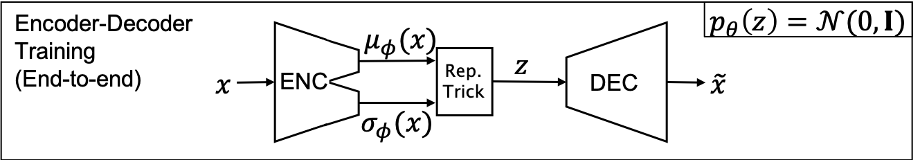
(a) VAE

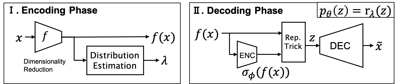
(b) P3GM

Figure 3: Model architectures of VAE and P3GM.

IV-A Overview

The generative model of PGM follows the same process as of VAE; first, latent variable $z$ is generated from prior distribution $p_{\theta}(z)$. Second, data $x$ is generated from posterior distribution $p_{\theta}(x|z)$. Then, we introduce an approximation $q_{\phi}(z|x)$ of $p_{\theta}(z|x)$ to derive $\mathcal{L}_{\text{ELBO}}$ (Equation (1)), which enables maximization of the likelihood of the given dataset. We will refer to $q_{\phi}(z|x)$ as a probabilistic encoder because $q_{\phi}(z|x)$ produces the distribution over the space of $z$ given data $x$. In a similar vein, we will refer to $p_{\theta}(x|z)$ as a probabilistic decoder because $p_{\theta}(x|z)$ produces the distribution over the space of $x$ given a latent variable $z$. In this paper, we assume that the encoder and the decoder produce a Gaussian distribution for the reparametrization trick and the tractability. The main difference is in its training process shown in Figure 3 comparing with VAE. Intuitively, PGM first uses a dimensional reduction $f$ instead of the embedding of VAE, which we call Encoding Phase. Then, PGM trains the decoder using the fixed encoder by $f$, which we call Decoding Phase. In PGM, we assume a distribution for $p_{\theta}(z)$ different from VAE to fix a part of parameters trained in Decoding Phase. Through Encoding Phase, we can partially fix the encoder used in Decoding Phase. Then, we train the other parameters with the fixed encoder following the AEVB algorithm in Decoding Phase. The fixed encoder makes the AEVB algorithm stable even if we replace SGD with DP-SGD. This stability is the advantage of our two-phased model.

IV-B Encoding Phase

Through Encoding Phase, a part of parameters, concretely, $\mu_{\phi}(x)=\mathbb{E}[q_{\phi}(z|x)]$, becomes fixed. In other words, Encoding Phase partially fixes the encoder. Here, we explain how to fix the parameter before Decoding Phase.

The encoder’s purpose is to encode original data to the latent space so that the decoder can decode the encoded data to the original data. Another purpose of the encoder is to encode the data to a latent variable that follows some distribution so that the decoder can learn to decode the latent variable. Therefore, we can fix the encoder by finding an encoder achieving these two purposes.

First, we describe the ideal but unrealistic assumption to make it easy to understand PGM. The assumption is that the encoder encodes the data to the same data, which means that the encoded data is following the true distribution $p_{\theta^{\ast}}(x)$. Since the encoded data includes the same information as the original data and follows $p_{\theta^{\ast}}(x)$, this encoder satisfies the above two purposes. Thus, we can fix the encoder as this. Then, we train the decoder using the fixed encoder in Decoding Phase while assuming that the latent variable is following $p_{\theta^{\ast}}(x)$. In other words, we assume that the distribution of the latent variable $z$ $p_{\theta}(z)$ is identical to $p_{\theta^{\ast}}(x)$. We note that when the decoder is $p_{\theta}(x=\rm{x}|\it{z}=\rm{x})=1$, it holds that $p_{\theta}(x)=p_{\theta^{\ast}}(x)$. This means that sampling $z$ from $p_{\theta^{\ast}}(x)$ and decoding $z$ to $x$ with the decoder $p_{\theta}(x|z)$, we can generate data which follows the actual distribution $p_{\theta^{\ast}}(x)$.

However, since the actual parameter $\theta^{\ast}$ is not observed and is intractable, we cannot estimate $\theta^{\ast}$, encode to $p_{\theta^{\ast}}(x)$, and sample $z$ from $p_{\theta^{\ast}}(x)$. Therefore, we approximate $p_{\theta^{\ast}}(x)$ by some tractable distribution to enable estimation, encoding, and sampling. However, due to the curse of dimensionality, it is hard to infer the parameter for high dimensional data that we want to tackle. Then, to solve this issue, we introduce a dimensionality reduction $f:\mathbb{R}^{d}\to\mathbb{R}^{d^{\prime}}$ where $d$ and $d^{\prime}$ are original and reduced dimensionality, respectively. We let $p^{f}_{\theta}(z)$ denote the distribution of $z=f(x)$ where $x$ follows $p_{\theta}(x)$. Then, $r_{\lambda}(z)$ denotes the approximation of $p^{f}_{\theta^{\ast}}(z)$ by some tractable distribution such as mixture of Gaussian (MoG). We fix the encoder to encode $x$ to data which follows $r_{\lambda}(z)$ by estimating the parameter $\lambda$.

As described above, the encoder’s purpose is to encode the data so that the decoder can decode the encoded data to the original data. From this purpose, the objective function for dimensionality reduction $f$ can be defined as follows:

$$\min_{f,g}\mathbb{E}_{x\sim p_{\theta^{*}}(x)}[\|x-g(f(x))\|^{2}_{2}]$$ (5)

where $g$ represents a reconstruction function of $f$. Intuitively, if there is a function $g$ where this value is small, data encoded by $f$ has the potential to be decoded to the original data. Conversely, if this is large, the decoder will not be able to decode the encoded data to the original data.

In this model, we assume that the mean of the true distribution of the latent variable $z$ given $\rm{x}$ is $f(\rm{x})$, i.e., $\mathbb{E}[p_{\theta}(z|x)]=f(x)$. Intuitively, this assumption means that PGM assumes that data $\rm{x}$ is generated from data whose dimensionality is reduced by $f$, i.e., $f(\rm{x})$. This assumption enables the fixing of the encoder as $\mu_{\phi}(\rm{x})=\it{f}(\rm{x})$, because the encoder is the approximation of $p_{\theta}(z|x)$.

Next, we estimate the distribution (i.e., $p^{f}_{\theta^{*}}(z)$) of the latent variable $z$ which is following the above generative process to feed and train the decoder with the estimated distribution. Since the estimated distribution $r_{\lambda}(z)$ should approximate the distribution well, the objective function to obtain the optimal $\lambda$ can be defined as follows:

$$\min_{\lambda}D_{\text{KL}}(p^{f}_{\theta^{*}}(z)||r_{\lambda}(z))$$ (6)

where $D_{\text{KL}}$ represents the Kullback–Leibler divergence. We consider the ideal case where there are a dimensionality reduction $f$, a reconstruction function $g$ and approximation $r_{\lambda}(z)$, which satisfies that Equation (5) and Equation (6) are $0$. In this case, if the decoder can emulate $g$ (e.g., above example) by training, it holds that $p_{\theta}(x)=p_{\theta^{\ast}}(x)$, which means that the PGM generates data which follows the actual distribution $p_{\theta^{\ast}}(x)$.

We note that the variance $\sigma_{\phi}(x)$ of the decoder $q_{\phi}(z|x)$ is not fixed in Decoding Phase, which means that we simultaneously train a part of the encoder for the encoder to approximate $p_{\theta^{\ast}}(z|x)$.

The dimensionality reduction and estimation of the distribution of the latent variable (i.e., $\lambda$) cause privacy leak. However, by guaranteeing DP for each component, PGM satisfies DP from the composition theorem (we refer to Section II-C).

IV-C Decoding Phase

We optimize the rest of the parameters of the encoder and the decoder following the AEVB algorithm. Here, we explain how to optimize the parameters. $\mathcal{L}_{\text{ELBO}}$ on log-liklihood $\log p_{\theta}(x)$, which was explained in Section II-A, is approximated by a technique of Monte Carlo estimates.

$$\begin{split}\mathcal{L}_{\text{ELBO}}(\rm{x})\approx&\frac{1}{L}\sum^{L}_{l=1}\log p_{\theta}(x=\rm{x}|\it{z}=z_{i,l})\\ &-D_{\text{KL}}(\textit{q}_{\phi}(\it{z}|\it{x}=\rm{x})\|\textit{p}_{\theta}(\it{z}))\end{split}$$ (7)

where $L$ is the number of iterations for Monte Carlo estimates and $z_{i,l}$ is sampled from the encoder with $\rm x$ using the reparametrization trick (we refer to Section II-A). If $\mathcal{L}_{\text{ELBO}}$ is differentiable, we can optimize parameters w.r.t. $\mathcal{L}_{\text{ELBO}}$ using SGD. The first term is differentiable when we assume that $p_{\theta}(x|z)$ is a Bernoulli or Gaussian MLP depending on the type of data we are modeling. Since we assume that $p_{\theta}(z)$ is identical to $r_{\lambda}(z)$, we need to choose a model for $r_{\lambda}(z)$ which makes the second term differentiable.

IV-D Example of P3GM

We introduce a concrete realization of the privacy-preserved version of PGM, i.e., P3GM. Same as VAE, P3GM uses neural networks for $p_{\theta}(x|z)$ and $q_{\phi}(z|x)$. The neural networks output the mean and variance of the distributions.

Encoding Phase: We first describe how to estimate the distribution of the latent variable in a differentially private way. First, we need to decide the model of the distribution. The requirements are as follows:

1. The second term of Equation (7) can be analytically calculated and is differentiable.

2. The objective function (6) is small enough to approximately express the true distribution $p_{\theta^{\ast}}^{f}(z)$.

3. We can estimate the distribution with DP.

The most simple prior distribution which satisfies the requirements is Gaussian. However, depending on the data type, Gaussian may not be enough to approximate the true distribution (requirement 2). Then, we introduce MoG because MoG can preserve the local structure of the data distribution more than Gaussian. That is,

$$r_{\lambda}(z)=\text{MoG}(z;\lambda)$$

When we approximate the expectation in the KL term of Equation (6) by the average of all given data, we can formulate the objective function as follows:

$$\max_{\lambda}\Pi_{i=1}^{N}r_{\lambda}(f(\rm{x}^{(i)}))$$

This is the same as the objective function of the maximum likelihood estimation, so we can use EM-algorithm for the estimation of the parameter of MoG. Further, EM-algorithm can satisfy DP by adding Gaussian noise (requirement 3), which we introduced as DP-EM [37] in Section II-D.

KL divergence between two mixture of Gaussian $g(\pi_{a},\mu_{a},\sigma_{a})$ and $h(\pi_{b},\mu_{b},\sigma_{b})$ can be approximated as follows [23]:

$$\begin{split}&D_{\text{KL}}(g|h)\approx\\ &\sum_{a}\pi_{a}\log{\frac{\Sigma_{a^{\prime}}\pi_{a^{\prime}}\exp{(-D_{\text{KL}}(\mathcal{N}(\mu_{a^{\prime}},\sigma_{a^{\prime}})\|\mathcal{N}(\mu_{a},\sigma_{a})))}}{\Sigma_{b}\pi_{b}\exp{(-D_{\text{KL}}(\mathcal{N}(\mu_{a},\sigma_{a})\|\mathcal{N}(\mu_{b},\sigma_{b})))}}}\end{split}$$

Therefore, we can analytically calculate the second term of (7) using this approximation (requirement 1).

To avoid the curse of dimensionality in the estimation of GMM, we utilize the dimensional reduction technique. In a dimensionality reduction, we aim to minimize the objective function (5) with DP. We approximate it by the average of all given data.

$$\sum^{N}_{x_{i}}\frac{1}{N}\|x_{i}-g(f(x_{i}))\|^{2}_{2}$$

When $f$ is a linear transformation which is useful for DP, this is optimized by PCA. As described in Section II, PCA can satisfy DP (DP-PCA). Therefore, we introduce DP-PCA as a dimensionality reduction.

Decoding Phase: As described above, since the $\mathcal{L}_{\text{ELBO}}$ is differentiable, we can optimize parameters with DP-SGD. We show the pseudocode for P3GM in Algorithm 1. We refer to the detail of DP-SGD in Section II-D. In Algorithm 1, all parameters $\theta$ and $\phi$ are packed into $\theta$, for simplicity.

Input: $\mathbf{x}_{1},\dots,\mathbf{x}_{N}\in\bf{X}$, $\bm{\mu}_{X}$

Output: The model parameters $\theta_{T}$, the parameter of MoG $\lambda$

Parameter : reduced dimension $d^{\prime}$, privacy parameters in PCA, EM and SGD $\sigma_{p},\sigma_{e},\sigma_{s}$, learning rate $\eta_{t}$, batch size $B$, gradient norm bound $C$

1 $\Sigma$ $\leftarrow$ DP-PCA($\mathbf{x}_{1},\dots,\mathbf{x}_{N}$;$d^{\prime}$, $\sigma_{p}$)

2 $\hat{\mathbf{x}}_{1},\dots,\hat{\mathbf{x}}_{N}$ $\leftarrow$ dimensional reduction($\bf{X},\bm{\Sigma},\bm{\mu}_{X}$)

3 $\lambda$ $\leftarrow$ DP-EM($\hat{\mathbf{x}}_{1},\dots,\hat{\mathbf{x}}_{N}$;$\sigma_{e}$)

4 $p_{\theta}(z)\leftarrow\text{MoG}(z;\lambda)$

5 for $t\in[T]$ do

6       Take a random batch $B_{t}$ w/ sampling probability $B/N$

7       Compute gradient

8       For each $(\mathbf{x}_{b},\mathbf{\hat{x}}_{b})\in[B_{t}]$ compute $\mathbf{g}_{t}(\mathbf{x}_{b},\mathbf{\hat{x}}_{b})\leftarrow\nabla_{\theta_{t}}\mathcal{L}_{\text{ELBO}}(\theta_{t},\mathbf{x}_{b},\mathbf{\hat{x}}_{b},\lambda)$

9       Add noise and descent

10      

11      $\tilde{\mathbf{g}}_{t}\leftarrow\frac{1}{B}(\sum_{b\in[B_{t}]}\psi_{C}(\mathbf{g}_{t}(\mathbf{x}_{b},\mathbf{\hat{x}}_{b}))+\mathcal{N}(0,\sigma_{s}^{2}C^{2}\textbf{I}))$

12       $\theta_{t+1}\leftarrow\theta_{t}-\eta_{t}\tilde{\mathbf{g}}_{t}$

13      

return $\theta_{T}$, $\lambda$

Algorithm 1 P3GM

IV-E Data Synthesis using P3GM

The data synthesis of our model follows the two steps below:

1. Choose a latent vector $z$. $z\sim MoG(z;\lambda)$

2. Generate $\tilde{x}$ by decoding $z$. $\tilde{x}\sim p_{\theta}(x|z)$.

It is worth noting that since MoG approximates the distribution of real data, we can generate data in a similar mixing ratio of real data. By utilizing our model, we can share privatized data by releasing the model that satisfies DP. Due to the post-processing properties of DP, sampled data from the model with random seeds do not violate DP.

IV-F Privacy Analysis

As we described in Section II-D, P3GM consumes privacy budgets at three steps: PCA, EM-algorithm, and SGD, and we introduced the differentially private methods independently. We can simply compute the privacy budget for each component by zCDP and MA, as described in the corresponding paper, and we can adopt sequential composition for the three components as the baseline.

Beyond this simple composition, we here follow RDP to rigorously compute the composition, and meet the following theorem.

Theorem 4

P3GM satisfies ($\varepsilon$, $\delta$)-DP, for any $0<\delta<1$, $\alpha>1$, such that:

$$\varepsilon\leq\varepsilon_{p}(\alpha)+T_{s}\varepsilon_{rs}(\alpha)+T_{e}\varepsilon_{re}(\alpha)+\frac{\log 1/\delta}{\alpha-1}.$$ (8)

where $\varepsilon_{p}(\alpha)=\alpha/(2\sigma_{p}^{2})$, $\varepsilon_{rs}(\alpha)=MA_{\text{DP-SGD}}(\alpha-1)/(\alpha-1)$, $\varepsilon_{re}(\alpha)=MA_{\text{DP-EM}}(\alpha-1)/(\alpha-1)$, and, $T_{s}$ and $T_{e}$ are the number of iterations in DP-SGD and DP-EM, respectively. We refer to Section II-D for the definition of $MA_{\text{DP-SGD}}$ and $MA_{\text{DP-EM}}$.

Proof

We consider RDP for each component of P3GM. First, as described at DP-PCA in Section II-D, DP-PCA satisfies $(\alpha,\alpha/(2\sigma_{p}^{2}))$-RDP. Second, DP-SGD satisfies $(\alpha,\varepsilon_{rs}(\alpha))$-RDP in each step from Theorem 3 and Inequality (4). Third, as in the case of DP-SGD, DP-EM satisfies $(\alpha,\varepsilon_{re}(\alpha))$-RDP in each step from Theorem 3 and Inequality (3). At last, from the composition theorem (Theorem 1) in RDP, P3GM satisfies $(\alpha,\varepsilon_{p}(\alpha)+T_{s}\varepsilon_{rs}(\alpha)+T_{e}\varepsilon_{re}(\alpha))$-RDP. By conversion from RDP to DP from Theorem 2, we meet (8).

V Discussions

First, we theoretically discuss why the AEVB algorithm finds a better solution under differential privacy by adopting the two-phased training than the end-to-end training of VAE. Second, we discuss the parameter tuning.

V-A Solution Space Elimination

Here, we discuss the effect to the solution space by fixing the mean of the encoder to some constant value $\mu_{\phi}(x)=c_{x}$ (In this paper, we use the dimension reduced data of $x$ by PCA as $c_{x}$). If the encoder freezes the the mean, it only searches variances to fit the posterior distribution $q_{\phi}(z|x)$ to the prior distribution $p_{\theta}(z)$.

PGM optimizes only the variance $\sigma_{\phi}(x)$ and the parameters of the decoder $\theta$ with the assumption that $q_{\phi}(z|x)$ is a Gaussian distribution whose mean is a constant $c_{x}$. The loss function of PGM is as follows:

$$\begin{split}\mathcal{L}_{PGM}(x)=&-D_{\text{KL}}(\mathcal{N}(c_{x},\sigma_{\phi}(x))||p_{\theta}(z))\\ &+\int{\mathcal{N}(z;c_{x},\sigma_{\phi}(x))\log p_{\theta}(x|z)}dz\end{split}$$ (9)

Comparing with this, $c_{x}$ is not freezed, so the search space for the loss function in VAE is clearly bigger than PGM. Assuming $\mu_{\phi}(x),\sigma_{\phi}(x)$, and $\theta$ be any values and $p_{\theta}(z)$ of VAE and PGM be the same, the range of all possible solutions of VAE includes all possible solutions of PGM.

Furthermore, assuming that $\sigma(x)$ is a constant $s_{x}$, we can more eliminate the search space. The first term in Equation (9) becomes a constant, and this is identical to autoencoder (AE) when we set $s_{x}=0$. Intuitively, the decoder only learns to decode $c_{x}$ because the encoder is fixed to encode $x$ to $c_{x}$.

The elimination of the search space helps our model to discover solutions within a smaller number of iterations. Our experiments in Section VI will demonstrate this fact.

V-B Parameter setting

P3GM has many parameters that impact privacy and utility. Our unique parameters that differentiate one of VAE are the reduced dimensionality and the ratio of the privacy budget allocation. The reduced dimensionality should be higher to keep the information, but it should be small enough to estimate MoG effectively, and we found $[10,100]$ is better. The privacy budget allocation is also an important aspect because if the encoder fails to learn the encoding, the decoder will fail to learn the decoding, and vice verse. Through experiments, We found that the ratio $3:7$ of the allocation to the encoder and the decoder is the better choice. You can find more details for the experiments in Section VI-D and VI-E. However, we should have theoretically better parameters since we consume the privacy budget for the observation when we try a set of parameters to see accuracy, which remains for future work. We note that we can use Gupta’s technique to save the privacy budget [2, 22] because we do not need the output but only need accuracy to choose the better parameters.

VI Experiments

In this section, we report the results of the experimental evaluation of P3GM. For evaluating our model, we design the experiments to answer the following questions:

• How effective can the generated samples be used in data mining tasks?

• How efficient in constructing a differentially private model?

• How much privacy consumption can be reduced in the privacy compositions?

To empirically validate the effectiveness of synthetic data sampled from P3GM, we conducted two different experiments.

Classification: First, we train P3GM using a real training dataset and generate a dataset so that the label ratio is the same as the real training dataset, as we described in Section IV-E. Then, we train the multiple classifiers on the synthetic data and evaluate the classifiers on the real test dataset. For the evaluation of the binary classifiers, we use the area under the receiver operating characteristics curve (AUROC) and area under the precision recall curve (AUPRC). For the evaluation of the multi-class classifier, we use classification accuracy.

2-way marginals: The second experiment builds all 2-way marginals of a dataset [6]. We evaluate the difference between the 2-way marginals made by synthetic data and original data. We use the average of the total variation distance of all 2-way marginals to measure the difference (i.e., the average of the half of $L_{1}$ distance between the two distributions on the 2-way marginals).

Datasets. We use six real datasets as shown in Table III to evaluate the performance of P3GM. Each dataset has the following characteristic: Kaggle credit card fraud detection dataset (Kaggle Credit) is very unbalanced data which contains only $0.2\%$ positive data. UCI ISOLET and UCI Epileptic Seizure Recognition (ESR) dataset are higher-dimensional data whose sample sizes are small against the dimension sizes. Adult is a well known dataset to evaluate privacy preserving data publishing, data mining, and data synthesis. Adult includes 15 attributes with binary class. MNIST and Fashion-MNIST are datasets with $28\times 28$ gray-scale images and have a label form 10 classes. We use $90\%$ of the datasets as training datasets and the rest as test datasets.

Dataset	$N$	#feature	#class	%positive
Kaggle Credit [15]	284807	29	2	0.2
Adult	45222	15	2	24.1
UCI ISOLET	7797	617	2	19.2
UCI ESR	11500	179	2	20.0
MNIST	70000	784	10	-
Fashion-MNIST	70000	784	10	-

TABLE III: Datasets

	$\sigma_{s}$	learning rate	#epochs	batch size
Kaggle Credit	2.1	0.001	15	100
Adult	1.4	0.001	5	200
UCI ISOLET	1.6	0.001	2	100
UCI ESR	1.4	0.001	2	100
MNIST	1.4	0.001	4	300
Fashion MNIST	1.4	0.001	4	300

TABLE IV: Hyper-parameters for each dataset.

Implementations of Generative Models. The encoder has two FC layers of [$d,1000,d^{\prime}$] with ReLU as the activate function. $d$ is the dimensionality of data and $d^{\prime}$ is the reduced dimensionality. The decoder also has two FC layers with [$d^{\prime},1000,d$] with ReLU as the activate function. We show the hyper-parameters used in DP-SGD for each dataset in Table IV. For the Kaggle Credit dataset, we did not apply dimensionality reduction because this dataset is originally low dimensionality. For the other datasets, we did dimensionality reduction with reduced dimensionality $d_{p}=10$ and $\varepsilon_{p}=0.1$. We set $\sigma_{e}$ as $\varepsilon=1$ holds, $T_{e}=20$, the number of components of MoG as $d_{m}=3$, and we use the diagonal covariance matrix as the covariance matrix of MoG for the efficiency. We develop the above models by Python 3.6.9 and PyTorch 1.4.0 [38].

Implementations of Classifiers. For table datasets, we use four different classifiers, LogisticRegression (LR), AdaBoostClassifier (AB) [19], GradientBoostingClassifier (GBM) [20], and XgBoost (XB) [13] from Python libraries, scikit-learn 0.22.1, and xgboost 0.90. We set the parameters of sklearn.GradientBoostingClassifier as max_features=”sqrt”, max_depth=8, min_samples_leaf=50 and min_samples_split=200. Other parameters are set to default. For image datasets, we train a CNN for the classification tasks using Softmax. The model has one Convolutional network with 28 kernels whose size is (3,3) and MaxPooling whose size is (2,2) and two FC layers with [128, 10]. We use ReLU as the activate function and apply dropout in FC layers.

Competitors. We compare P3GM with PrivBayes [44], DP-GM [5], Ryan’s algorithm [31] and DP-VAE.

Reproducibility. We will make the code public for reproducibility. Under the review process, our code is available on the anonymous repository.

	AUROC			AUPRC
	VAE	PGM	P3GM	VAE	PGM	P3GM
LR	0.9617	0.9454	0.9264	0.6542	0.6865	0.6750
AB	0.9599	0.9330	0.9026	0.5737	0.6528	0.6474
GBM	0.9619	0.9442	0.9182	0.6838	0.6734	0.6645
XB	0.9395	0.9321	0.9026	0.2745	0.6469	0.6218

TABLE V: Accuracy comparison with non-private models. PGM and P3GM show relatively close accuracy against VAE.

Dataset	AUROC					AUPRC
	PrivBayes	Ryan’s	DP-GM	P3GM	original	PrivBayes	Ryan’s	DP-GM	P3GM	original
Kaggle Credit	0.5520	0.5326	0.8805	0.8991	0.9663	0.2084	0.2503	0.3301	0.6586	0.8927
UCI ESR	0.5377	0.5757	0.4911	0.8801	0.8698	0.5419	0.4265	0.3311	0.7672	0.8098
Adult	0.8530	0.5048	0.7806	0.8214	0.9119	0.6374	0.2584	0.4502	0.5972	0.7844
UCI ISOLET	0.5100	0.5326	0.4695	0.7498	0.9891	0.2084	0.2099	0.1816	0.3950	0.9623

TABLE VI: Performance comparison on four real datasets. Each score is the average AUROC or AUPRC over four classifiers listed in Table V. P3GM outperforms other two differentially private models on three datasets.

VI-A Effectiveness in Data Mining Tasks

We evaluate how effective can the generated samples be used in several data mining tasks. We also empirically evaluate the trade-off between utility and the privacy protection level.

Against non-private models in table data. Here, we show that P3GM with ($1,10^{-5}$)-DP does not cause much utility loss than non-private models: PGM and VAE. Table V presents the results on the Kaggle Credit dataset. As listed in Table V, we utilized four different classifiers. Comparing PGM with VAE, it is said that PGM has similar expression power as VAE. Comparing P3GM with non-private methods, in spite of the noise for DP, we can see that scores of P3GM do not significantly decrease, which shows the tolerance to the noise.

Comparison with private models in table data. Next, we perform comparative analysis for P3GM, PrivBayes, and DP-GM with ($1,10^{-5}$)-DP on four real datasets. In Table VI, we give the performance on each dataset averaged across these four different classifiers as well as Table V. P3GM outperforms the other two differentially private models on three datasets in AUROC and AUPRC. However, there is much degradation on the UCI ISOLET dataset. This is because the smaller data size causes more noise for DP and the high dimensionality makes it difficult to find a good solution in the small number of iterations. On the Adult dataset, PrivBayes shows a little better performance than P3GM due to the simpler model. However, PrivBayes only performs well for datasets having simple dependencies and a small number of features like the Adult dataset. Regarding the high dimensional data, our method is significantly better than PrivBayes. Ryan’s algorithm does not perform well on this task. Since Ryan’s algorithm constructs data from limited information (i.e., 1, 2, and 3-way marginals), Ryan’s algorithm cannot reconstruct the essential information which is required for the classification task.

Classification on image datasets. We perform comparative analysis with DP-GM and PrivBayes on MNIST and Fashion-MNIST, whose data is high-dimensional. In Table VII, we give the classification accuracies of classifiers trained on each synthetic data. P3GM results in much better results than DP-GM and PrivBayes, which shows the robustness to high-dimensional data. Moreover, P3GM shows around 6% and 5% less accuracy than VAE on MNIST and Fashion-MNIST, respectively, under ($\varepsilon,\delta$)=($1,10^{-5}$). The accuracies are relatively close to VAEs even P3GM satisfied the differential privacy. Back to Figure 2, we also displayed generated samples from our model and competitors. As we can see, P3GM can generate images that are visually closer to VAE while satisfying differential privacy.

Dataset	VAE	DP-GM	PrivBayes	Ryan’s	P3GM
MNIST	0.8571	0.4973	0.0970	0.2385	0.7940
Fashion	0.7854	0.5200	0.0996	0.2408	0.7485

TABLE VII: Classification accuracies on image datasets.

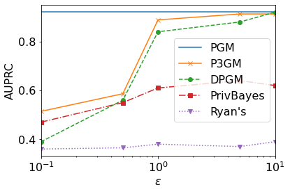
(a) AUPRC

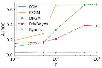
(b) AUROC

Figure 4: Utility in fraud detection (Kaggle Credit).

Varying privacy levels. Here, we measure our proposed method’s performance when we vary the privacy protection level $\varepsilon$. In Figure 4, we plot AUROC and AUPRC of classifiers trained using synthetic Kaggle Credit dataset generated by P3GM, DP-GM and PrivBayes w.r.t. each $\varepsilon$ with $\delta=10^{-5}$. PrivBayes does not show high scores even when $\varepsilon$ is large, which means that PrivBayes does not have enough capacity to generate datasets whose dependencies of attributes are complicated, such as Kaggle Credit. Also, as we can see, although DP-GM rapidly degrades the scores as $\varepsilon$ becomes smaller, the ones of P3GM does not significantly decrease. This result shows that P3GM is not significantly influenced by the noise for satisfying DP.

Varying degree of dimensionality reduction. Here, we empirically explain how the number of components of PCA affects the performance of P3GM. Figure 6 shows the results on the MNIST. As we can see, the number of components ($d_{p}$) affects performance. Too much high dimensionality makes (DP-)EM algorithm ineffective due to the curse of dimensionality. Too much small dimensionality lacks the expressive power for embedding. From the result, $d_{p}=[10,100]$ looks a good solution with balancing the accuracy and the dimensionality reduction on the MNIST dataset.

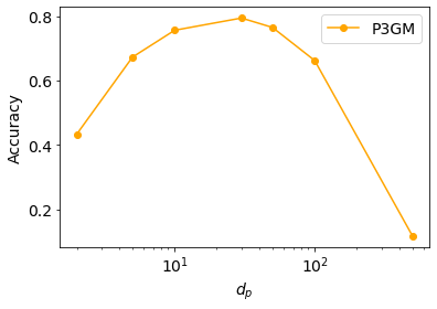
Figure 5: Reducing dimension improves accuracy (MNIST).

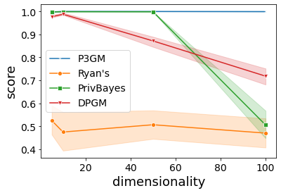
Figure 6: Only P3GM can handle high-dimensionality.

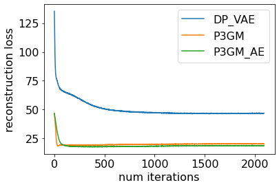
(a) Reconstruction loss (MNIST).

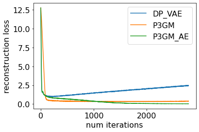
(b) Reconstruction loss (Kaggle Credit)

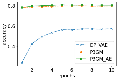
(c) Classification accuracy (MNIST).

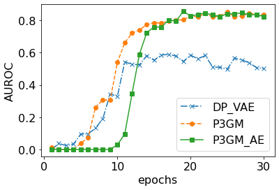
(d) AUROC (Kaggle Credit)

Figure 7: P3GM demonstrates higher learning efficiency than DP-VAE. More simple model increases more learning efficiency.

VI-B Learning Efficiency

Here, we measure the learning efficiency of the proposed method. As discussed in Section V, we can interpret that our model reduces the search space to accelerate the convergence speed. We empirically demonstrate it in Figure 7. Here, let P3GM (AE) denote P3GM with fixing $\sigma_{\phi}(x)=0$.

In Figure 7a and Figure 7b, our proposed method shows faster converegence than naïve method (DP-VAE) in the reconstruction loss (the first term of (7)). For these two datasets, P3GM met convergences at earlier epochs than DP-VAE. In Figure 7b, the loss of DP-VAE is decreased gradually in the long term but shows fluctuations in the short term. In contrast, P3GM shows monotonic decreases in reconstruction loss. This is due to the solution space elimination by freezing the encoder in our model.

We plot the performance in each epoch to see the convergence speed of the models in Figure 7c and Figure 7d, which shows that the performance with the smaller search space also converges faster. Figure 7c shows the classification accuracy with MNIST dataset and Figure 7d shows the AUROC with the Kaggle Credit dataset. In both results, P3GM (AE) converged at the earliest iteration in those three methods. While at the end of iterations, P3GM shows the best results, and P3GM (AE) is the second-best. This is because the search space of P3GM is larger than P3GM (AE), so it can find the better solution. In a similar vein, VAE can find a better solution since the search space of VAE is larger than P3GM, but it will cost a non-acceptable privacy budget. P3GM balances the search space size and the cost of the privacy budget.

Dataset	PrivBayes	Ryan’s	DP-GM	P3GM
Kaggle Credit	0.9326	0.0082	0.1345	0.2411
UCI ESR	0.8793	0.0936	0.6083	0.0654
Adult	0.0752	0.0494	0.2672	0.3867
UCI ISOLET	0.5324	0.1611	0.6855	0.3029

TABLE VIII: Avg. total variational distance of 2-way marginals.

VI-C Accuracy of 2-way marginals

Table VIII shows the results of the 2-way marginals experiment, which is one of the NIST competition measures. Here, since the total variation distance represents the error of the distribution (of 2-way marginals) made by the synthetic data, we can see that Ryan’s algorithm performs the best. This is because Ryan’s algorithm directly computes the crucial 2-way marginals with the Gaussian mechanism, which leads to the win in the NIST competition. The direct method, such as Ryan’s algorithm, is useful for a simple task like building a 2-way distribution. Still, it loses the complex information such as the dependencies in multiple attributes, which results in the worse result in the classification task. Although P3GM is inferior to Ryan’s algorithm for this task, P3GM keeps the 2-way marginal distribution better than PrivBayes and DP-GM for datasets with high dimensionalities.

VI-D Dimensionality

We here experimentally show the impact to the algorithms by a dimensionality. We make a dataset by sampling from two Gaussian distributions whose means are $(1,1,\dots,1)$ and $(-1,-1,\dots,-1)$ and whose covariance matrices are the identity matrices and attach different labels. From the two Gaussians, we generate synthesized datasets with $\epsilon=1$ varying the dimensionality from $5$ to $100$, and measure the AUROC in binary classifications for the datasets. Figure 6 shows these scores of each method. P3GM can handle high-dimensinality, but the others are highly depending on the dimensionality.

VI-E Privacy budget allocation

P3GM has two components: Encoding Phase (i.e., DP-PCA and DP-EM) and Decoding Phase (i.e., DP-SGD). So far, we used the fixed privacy budget allocation for the two components. Here, we experimentally explore the P3GM’s perfomance variations when varying the ratio of the allocation while keeping the total privacy budget to $1$. We plot the result for the Adult dataset in Figure 9. We can see that the score is top when the ratio is from $0.1$ to $0.3$. However, it is interesting to explore a theoretically better allocation ratio rather than this empirical result, which remains for future work.

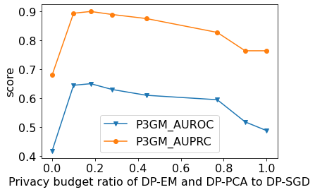
Figure 8: Performance in varying privacy budget allocations.

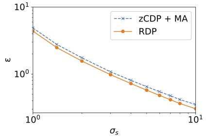
Figure 9: Privacy composition in RDP saves privacy budgets.

VI-F Privacy Composition

In this paper, we introduced the composition of privacy loss based on RDP. Here, we show that our composition method more rigorously accountants each privacy budget than the baseline. We use zCDP for DP-EM and MA for DP-SGD as the baseline, which is proposed composition methods in the corresponding papers. Figure 9 shows the computed value of $\varepsilon$ by each method, varying the amount of noise for DP-SGD. We freeze the amount of noise for MA. Our composition based on RDP results in a smaller value of $\epsilon$ than the baseline. Thus our method can compute the privacy composition in a lean way.

VII Conclusion

This paper addressed the question, how can we release a massive volume of sensitive data while mitigating privacy risks? Particularly, to construct a differentially private deep generative model for high dimensional data, we introduced a novel model, P3GM. The proposed model P3GM hires an encoder-decoder framework as well as VAE but employs a different algorithm that introduces a two-phase process for training the model to increase the robustness to the differential privacy constraint. We also gave a theoretical analysis of how effectively our method reduces complexity comparing with VAE. We further provided an extensive experimental evaluation of the accuracy of the synthetic datasets generated from P3GM. Our experiments showed that data mining tasks using data generated by P3GM are more accurate than existing techniques in many cases. The experiments also demonstrated that P3GM generated samples with less noise and resulted in higher utility in classification tasks than competitors. Exploring the the optimality of parameters, dimensionality reduction (Equation 5), and estimation of the latent distribution (Equation 6) remains for future works.

References

- [1] https://ergodicity.net/2017/04/07/retraction-for-symmetric-matrix-perturbation-for-differentially-private-principal-component-analysis-icassp-2016/.
- [2] M. Abadi, A. Chu, I. Goodfellow, H. B. McMahan, I. Mironov, K. Talwar, and L. Zhang. Deep learning with differential privacy. In Proceedings of the 2016 ACM SIGSAC Conference on Computer and Communications Security, pages 308–318. ACM, 2016.
- [3] J. M. Abowd. The us census bureau adopts differential privacy. In Proceedings of the 24th ACM SIGKDD International Conference on Knowledge Discovery & Data Mining, pages 2867–2867, 2018.
- [4] O. Abul, F. Bonchi, and M. Nanni. Never walk alone: Uncertainty for anonymity in moving objects databases. In 2008 IEEE 24th international conference on data engineering, pages 376–385. Ieee, 2008.
- [5] G. Acs, L. Melis, C. Castelluccia, and E. De Cristofaro. Differentially private mixture of generative neural networks. IEEE Transactions on Knowledge and Data Engineering, 31(6):1109–1121, 2018.
- [6] B. Barak, K. Chaudhuri, C. Dwork, S. Kale, F. McSherry, and K. Talwar. Privacy, accuracy, and consistency too: a holistic solution to contingency table release. In Proceedings of the twenty-sixth ACM SIGMOD-SIGACT-SIGART symposium on Principles of database systems, pages 273–282, 2007.
- [7] V. Bindschaedler, R. Shokri, and C. A. Gunter. Plausible deniability for privacy-preserving data synthesis. Proceedings of the VLDB Endowment, 10(5):481–492, 2017.
- [8] M. Bun and T. Steinke. Concentrated differential privacy: Simplifications, extensions, and lower bounds. In Theory of Cryptography Conference, pages 635–658. Springer, 2016.
- [9] U. S. C. Bureau. Disclosure avoidance and the 2020 census. https://www.census.gov/about/policies/privacy/statistical_safeguards/disclosure-avoidance-2020-census.html, 2019.
- [10] T. Cao, A. Bie, A. Vahdat, S. Fidler, and K. Kreis. Don’t generate me: Training differentially private generative models with sinkhorn divergence. Advances in Neural Information Processing Systems, 34, 2021.
- [11] K. Chaudhuri, J. Imola, and A. Machanavajjhala. Capacity bounded differential privacy. In Advances in Neural Information Processing Systems, pages 3469–3478, 2019.
- [12] R. Chen, Q. Xiao, Y. Zhang, and J. Xu. Differentially private high-dimensional data publication via sampling-based inference. In Proceedings of the 21th ACM SIGKDD International Conference on Knowledge Discovery and Data Mining, pages 129–138. ACM, 2015.
- [13] T. Chen and C. Guestrin. Xgboost: A scalable tree boosting system. In Proceedings of the 22nd acm sigkdd international conference on knowledge discovery and data mining, pages 785–794. ACM, 2016.
- [14] G. Cormode, T. Kulkarni, and D. Srivastava. Constrained private mechanisms for count data. IEEE Transactions on Knowledge and Data Engineering, 2019.
- [15] A. Dal Pozzolo, O. Caelen, R. A. Johnson, and G. Bontempi. Calibrating probability with undersampling for unbalanced classification. In 2015 IEEE Symposium Series on Computational Intelligence, pages 159–166. IEEE, 2015.
- [16] J. Domingo-Ferrer, K. Muralidhar, and M. Bras-Amorós. General confidentiality and utility metrics for privacy-preserving data publishing based on the permutation model. IEEE Transactions on Dependable and Secure Computing, 2020.
- [17] C. Dwork. Differential privacy. In Proceedings of the 33rd international conference on Automata, Languages and Programming-Volume Part II, pages 1–12. Springer-Verlag, 2006.
- [18] C. Dwork, K. Talwar, A. Thakurta, and L. Zhang. Analyze gauss: optimal bounds for privacy-preserving principal component analysis. In Proceedings of the forty-sixth annual ACM symposium on Theory of computing, pages 11–20, 2014.
- [19] Y. Freund, R. E. Schapire, et al. Experiments with a new boosting algorithm. In icml, volume 96, pages 148–156. Citeseer, 1996.
- [20] J. H. Friedman. Greedy function approximation: a gradient boosting machine. Annals of statistics, pages 1189–1232, 2001.
- [21] I. Goodfellow, J. Pouget-Abadie, M. Mirza, B. Xu, D. Warde-Farley, S. Ozair, A. Courville, and Y. Bengio. Generative adversarial nets. In Advances in neural information processing systems, pages 2672–2680, 2014.
- [22] A. Gupta, K. Ligett, F. McSherry, A. Roth, and K. Talwar. Differentially private combinatorial optimization. In Proceedings of the twenty-first annual ACM-SIAM symposium on Discrete Algorithms, pages 1106–1125. SIAM, 2010.
- [23] J. R. Hershey and P. A. Olsen. Approximating the kullback leibler divergence between gaussian mixture models. In 2007 IEEE International Conference on Acoustics, Speech and Signal Processing-ICASSP’07, volume 4, pages IV–317. IEEE, 2007.
- [24] W. Jiang, C. Xie, and Z. Zhang. Wishart mechanism for differentially private principal components analysis. In Thirtieth AAAI Conference on Artificial Intelligence, 2016.
- [25] J. Jordon, J. Yoon, and M. van der Schaar. Pate-gan: generating synthetic data with differential privacy guarantees. In International Conference on Learning Representations, 2018.
- [26] D. P. Kingma, T. Salimans, R. Jozefowicz, X. Chen, I. Sutskever, and M. Welling. Improved variational inference with inverse autoregressive flow. In Advances in neural information processing systems, pages 4743–4751, 2016.
- [27] D. P. Kingma and M. Welling. Auto-encoding variational bayes. arXiv preprint arXiv:1312.6114, 2013.
- [28] I. Kotsogiannis, Y. Tao, X. He, M. Fanaeepour, A. Machanavajjhala, M. Hay, and G. Miklau. Privatesql: a differentially private sql query engine. Proceedings of the VLDB Endowment, 12(11):1371–1384, 2019.
- [29] Y.-H. Kuo, C.-C. Chiu, D. Kifer, M. Hay, and A. Machanavajjhala. Differentially private hierarchical count-of-counts histograms. Proceedings of the VLDB Endowment, 11(11):1509–1521, 2018.
- [30] A. Machanavajjhala, J. Gehrke, D. Kifer, and M. Venkitasubramaniam. l-diversity: Privacy beyond k-anonymity. In 22nd International Conference on Data Engineering (ICDE’06), pages 24–24. IEEE, 2006.
- [31] R. McKenna. rmckenna - differential privacy synthetic data challenge algorithm. https://github.com/usnistgov/PrivacyEngCollabSpace/tree/master/tools/de-identification/Differential-Privacy-Synthetic-Data-Challenge-Algorithms/rmckenna, 2019.
- [32] F. D. McSherry. Privacy integrated queries: an extensible platform for privacy-preserving data analysis. In Proceedings of the 2009 ACM SIGMOD International Conference on Management of data, pages 19–30, 2009.
- [33] I. Mironov. Rényi differential privacy. In 2017 IEEE 30th Computer Security Foundations Symposium (CSF), pages 263–275. IEEE, 2017.
- [34] J. Murtagh and S. Vadhan. The complexity of computing the optimal composition of differential privacy. In Theory of Cryptography Conference, pages 157–175. Springer, 2016.
- [35] NIST. Differential privacy synthetic data challenge. https://www.topcoder.com/community/data-science/Differential-Privacy-Synthetic-Data-Challenge, 2018.
- [36] N. Papernot, M. Abadi, U. Erlingsson, I. Goodfellow, and K. Talwar. Semi-supervised knowledge transfer for deep learning from private training data. arXiv preprint arXiv:1610.05755, 2016.
- [37] M. Park, J. Foulds, K. Choudhary, and M. Welling. Dp-em: Differentially private expectation maximization. In Artificial Intelligence and Statistics, pages 896–904, 2017.
- [38] A. Paszke, S. Gross, S. Chintala, G. Chanan, E. Yang, Z. DeVito, Z. Lin, A. Desmaison, L. Antiga, and A. Lerer. Automatic differentiation in pytorch. 2017.
- [39] C. Sahin, T. Allard, R. Akbarinia, A. El Abbadi, and E. Pacitti. A differentially private index for range query processing in clouds. In 2018 IEEE 34th International Conference on Data Engineering (ICDE), pages 857–868. IEEE, 2018.
- [40] L. Sweeney. k-anonymity: A model for protecting privacy. International Journal of Uncertainty, Fuzziness and Knowledge-Based Systems, 10(05):557–570, 2002.
- [41] Y.-X. Wang, B. Balle, and S. Kasiviswanathan. Subsampled r’enyi differential privacy and analytical moments accountant. arXiv preprint arXiv:1808.00087, 2018.
- [42] L. Xie, K. Lin, S. Wang, F. Wang, and J. Zhou. Differentially private generative adversarial network. arXiv preprint arXiv:1802.06739, 2018.
- [43] J. Xu, Z. Zhang, X. Xiao, Y. Yang, G. Yu, and M. Winslett. Differentially private histogram publication. The VLDB Journal, 22(6):797–822, 2013.
- [44] J. Zhang, G. Cormode, C. M. Procopiuc, D. Srivastava, and X. Xiao. Privbayes: private data release via bayesian networks. In Proceedings of the 2014 ACM SIGMOD International Conference on Management of Data, pages 1423–1434, 2014.
- [45] J. Zhang, X. Xiao, and X. Xie. Privtree: A differentially private algorithm for hierarchical decompositions. In Proceedings of the 2016 International Conference on Management of Data, pages 155–170. ACM, 2016.