Adaptive Parameter Tuning for Reachability Analysis of Linear Systems

Abstract

Despite the possibility to quickly compute reachable sets of large-scale linear systems, current methods are not yet widely applied by practitioners. The main reason for this is probably that current approaches are not push-button-capable and still require to manually set crucial parameters, such as time step sizes and the accuracy of the used set representation—these settings require expert knowledge. We present a generic framework to automatically find near-optimal parameters for reachability analysis of linear systems given a user-defined accuracy. To limit the computational overhead as much as possible, our methods tune all relevant parameters during runtime. We evaluate our approach on benchmarks from the ARCH competition as well as on random examples. Our results show that our new framework verifies the selected benchmarks faster than manually-tuned parameters and is an order of magnitude faster compared to genetic algorithms.

I Introduction

Reachability analysis is one of the main techniques to formally verify the correctness of mixed discrete/continuous systems: It computes the set of reachable states of a system for a set of uncertain initial states as well as uncertain inputs. If the reachable set does not intersect the unsafe regions defined by a given safety property, that property is satisfied.

Exact reachable sets can only be computed for a limited class of systems [1]. In the remaining cases, one calculates over-approximations whose tightness is strongly influenced by algorithm parameters; unlike model parameters, these parameters have no relation to the considered model.

Due to large over-approximations resulting from poor algorithm parameters, reachability analysis may fail to prove a safety property even though the property is satisfied by the exact reachable set. We address this problem by proposing a novel generic framework to automatically tune all algorithm parameters for reachability analysis of linear continuous time-invariant systems during runtime respecting a user-defined error bound. Our framework can be used for different reachability algorithms and for different set representations.

State of the Art

Reachability algorithms for linear continuous systems are mainly based on the propagation of reachable sets for multiple time steps until reaching a fixed point or a user-defined time horizon. Propagation-based techniques have been extensively investigated [2, 3, 4, 5, 6, 7] using tools such as CORA [8], Flow* [9], XSpeed [10], SpaceEx [7], and JuliaReach [11]. A further method is to compute reachable sets using simulations [12, 13], which is implemented in the tool HyLAA [14]. The used set representation is another distinctive feature besides the method to compute reachable sets. Many different set representations have been researched, including polytopes [7], zonotopes [5], ellipsoids [15], griddy polyhedra [16], star sets [12], support functions [17], and constrained zonotopes [18].

Previous approaches for automated parameter tuning mainly focused on the time step size: Numerical ODE solvers often compute different solutions in parallel and decrease the time step size if the difference between solutions exceeds a certain threshold [19, 20]. Furthermore, several automated time step adaptation strategies have been developed for guaranteed integration methods that enclose only a single trajectory rather than a set of trajectories [21, 22, 23]. For reachability analysis, only a few methods automatically set the time step size. The approach in [7] chooses the time step size automatically in order to keep the error in a user-defined direction below a user-defined bound. Furthermore, the approach in [24] automatically chooses suitable time step sizes so that the Hausdorff distance between the exact reachable set and the computed over-approximation stays below a certain threshold. So far, there is no approach that considers all algorithm parameters.

Contributions

We introduce a novel generic framework that automatically tunes all algorithm parameters of a reachability algorithm so that the over-approximation error stays below a user-defined threshold. This generalized framework can be applied to many different reachability algorithms and we show that our self-parametrization approach always converges if the reachability algorithm satisfies certain requirements.

After introducing some preliminaries in Sec. II, we present our generic framework in Sec. III. In Sec. IV, we demonstrate the implementation of our framework for a specific reachability algorithm. Finally, the evaluation of our implementation on several numerical examples in Sec. V demonstrates the fully automated computation of tight over-approximations of reachable sets with only little computational overhead.

II Preliminaries

To concisely explain the novelties of our paper, we first introduce some preliminaries.

II-A Notation

Vectors are denoted by lower-case letters and matrices by upper-case letters. Square matrices of zeros are denoted by ${0_{n}\in\mathbb{R}^{n\times n}}$ and the identity matrix by ${I_{n}\in\mathbb{R}^{n\times n}}$. Given a vector ${a\in\mathbb{R}^{n}}$, $a_{i}$ refers to the $i$-th entry. An $n$-dimensional interval is denoted by $\mathcal{I}{}=[\underaccent{\bar}{l},\bar{l}]\subset\mathbb{R}^{n}$, where $\underaccent{\bar}{l}_{i}\leq\bar{l}_{i}$, $\forall i\in\{1,...,n\}$. The operators $\inf(\mathcal{I}{})=\underaccent{\bar}{l}\in\mathbb{R}^{n}$ and $\sup(\mathcal{I}{})=\bar{l}\in\mathbb{R}^{n}$ return the infimum and the supremum of an interval $\mathcal{I}{}=[\underaccent{\bar}{l},\bar{l}]$. Interval matrices are denoted in boldface: $\mathbf{I}=[\underaccent{\bar}{I},\bar{I}]\in\mathbb{R}^{m\times n}$, where $\inf(\mathbf{I})=\underaccent{\bar}{I}\in\mathbb{R}^{m\times n}$ and $\sup(\mathbf{I})=\bar{I}\in\mathbb{R}^{m\times n}$. The linear map is written without any operator between the operands, the Minkowski sum is denoted by $\oplus$, and the convex hull operator by $\texttt{conv}\big{(}\cdot\big{)}$.

II-B Reachability Analysis of Linear Systems

The presented technique for adaptive self-parametrization is applied to linear time-invariant (LTI) systems with initial states bounded by $\mathcal{X}^{0}{}\subset\mathbb{R}^{n}$ and inputs bounded by $\mathcal{U}{}\subset\mathbb{R}^{n}$:

$$\begin{split}&\dot{x}(t)=Ax(t)+u(t)\;,\\ &\text{with}\quad x(0)\in\mathcal{X}^{0}{}\subset\mathbb{R}^{n},\;\forall t:u(t)\in\mathcal{U}{}\subset\mathbb{R}^{n}\;,\end{split}$$ (1)

where $A\in\mathbb{R}^{n\times n}$ is the system matrix, $x(t)\in\mathbb{R}^{n}$ is the state vector, and $u(t)\in~{}\mathbb{R}^{n}$ is the input vector.

The above system also encompasses systems $\dot{x}(t)=Ax(t)+B\tilde{u}(t)$, where $B\in\mathbb{R}^{m\times n}$ is the input matrix, as we can set $\mathcal{U}=\{B\tilde{u}\,|\,\tilde{u}\in\mathcal{D}\subset\mathbb{R}^{m}\}$. Let us introduce $\xi\big{(}t;x_{0},u(\cdot)\big{)}$ as the solution of (LABEL:eq:LTI) to define the exact reachable set $\mathcal{R}_{\text{ex}}\big{(}[0,T]\big{)}$ of (LABEL:eq:LTI) over the time horizon $t\in[0,T]$:

$$\mathcal{R}_{\text{ex}}\big{(}[0,T]\big{)} =\Big{\{}\xi\big{(}t;x_{0},u(\cdot)\big{)}\,\Big{|}\,x_{0}\in\mathcal{X}^{0}{},$$

$$\qquad\quad\forall\tau\in[0,t]:u(\tau)\in\mathcal{U}{},\,t\in[0,T]\Big{\}}\;.$$

Due to the superposition principle, $\mathcal{R}_{\text{ex}}\big{(}[0,T]\big{)}$ is the sum of the homogeneous solution $\mathcal{H}^{\mathcal{R}}_{\text{ex}}\big{(}[0,T]\big{)}$ and the inhomogeneous solution $\mathcal{P}^{\mathcal{R}}_{\text{ex}}\big{(}[0,T]\big{)}$ [25, (3.6)]:

$$\mathcal{R}_{\text{ex}}\big{(}[0,T]\big{)}=\mathcal{H}^{\mathcal{R}}_{\text{ex}}\big{(}[0,T]\big{)}\oplus\mathcal{P}^{\mathcal{R}}_{\text{ex}}\big{(}[0,T]\big{)}\;,$$

where

$$\mathcal{H}^{\mathcal{R}}_{\text{ex}}\big{(}[0,T]\big{)} =\Big{\{}e^{At}x_{0}\,\Big{|}\,x_{0}\in\mathcal{X}^{0}{},\,t\in[0,T]\Big{\}}\;,$$

$$\mathcal{P}^{\mathcal{R}}_{\text{ex}}\big{(}T\big{)} =\bigg{\{}\int_{0}^{T}e^{A(T-\tau)}u(\tau)\mathrm{d}\tau\,\bigg{|}\,u(\tau)\in\mathcal{U}{}\bigg{\}}\;.$$

If $0\in\mathcal{U}{}$, $\mathcal{P}^{\mathcal{R}}_{\text{ex}}\big{(}[0,T]\big{)}=\mathcal{P}^{\mathcal{R}}_{\text{ex}}\big{(}T\big{)}$ and the extension for $0\notin\mathcal{U}{}$ is shown in [25, Sec. 3.2.2]. To limit the over-approximation, the time horizon $[0,T]$ is discretized by $K$ time steps $\Delta t_{i}=t_{i+1}-t_{i}>0$, $i\in\{0,...,K-1\}$, where $T=\sum_{i=0}^{K-1}\Delta t_{i}$ so that $\bigcup_{i=0}^{K-1}~{}\mathcal{R}\big{(}[t_{i},t_{i+1}]\big{)}$. We compute the reachable sets from the first time interval [26, Chap. 4]:

$$\begin{split}\mathcal{H}^{\mathcal{R}}\big{(}[t_{i},t_{i+1}]\big{)}&=e^{At_{i}}\mathcal{H}^{\mathcal{R}}\big{(}[0,\Delta t_{i}]\big{)}\;,\\ \mathcal{P}^{\mathcal{R}}\big{(}[0,t_{i+1}]\big{)}&=\mathcal{P}^{\mathcal{R}}\big{(}[0,t_{i}]\big{)}\oplus\underbrace{e^{At_{i}}\mathcal{P}^{\mathcal{R}}\big{(}[0,\Delta t_{i}]\big{)}}_{=:\,\mathcal{P}^{\mathcal{R}}{\textstyle(}[t_{i},t_{i+1}]{\textstyle)}}\;.\end{split}$$ (2)

This method adapts seamlessly to varying time step sizes, making it the preferred choice for adaptive parameter tuning compared to methods propagating the reachable set from the previous time step.

III Self-Parametrization

In this section, we introduce our novel algorithm for adaptive parameter tuning.

III-A Overview of Algorithm Parameters

The reachability algorithm from Sec. II-B depends on different algorithm parameters, which we divide into:

• Time Step Size: The propagation in (2) can be applied to any series of $\Delta t_{i}$ adding up to $T$. Large $\Delta t$ speed up the computation, while small $\Delta t$ increase the precision.

• Propagation Parameters: The tightness of the computed reachable sets also depends on parameters approximating the dynamics $\Phi_{\text{prop}}{}$, e.g., determining the precision of computing $e^{At}$. We introduce the operator $\texttt{incr}(\Phi_{\text{prop}}{})$ which increments the parameters $\Phi_{\text{prop}}{}$ towards values which result in a tighter reachable set, as well as the operator $\texttt{reset}(\Phi_{\text{prop}}{})$ which resets $\Phi_{\text{prop}}{}$ to the coarsest setting.

• Set Representation: We denote the number of scalar values needed to describe a set by $\Phi_{\text{set}}{}$. Let us introduce the operator $\texttt{decr}(\Phi_{\text{set}}{})$ which decreases $\Phi_{\text{set}}{}$. If $\Phi_{\text{set}}{}$ has reached its minimum, it returns $\texttt{decr}(\Phi_{\text{set}}{})=\Phi_{\text{set}}{}$. We denote the over-approximation of a set $\mathcal{S}{}$ by reducing its number of parameters to a desired value $\Phi_{\text{set}}{}$ by the operator $\texttt{red}\big{(}\mathcal{S}{},\Phi_{\text{set}}{}\big{)}$.

III-B Error measures

As we can only compute over-approximations, we are interested in measuring the over-approximation error. Let the reachable set $\mathcal{H}^{\mathcal{R}}{}$ consist of summands, e.g., $\mathcal{H}^{\mathcal{R}}{}=\mathcal{H}^{\mathcal{R}}{}^{(1)}\oplus...\oplus\mathcal{H}^{\mathcal{R}}{}^{(\nu)}$, as shown for a concrete implementation in Sec. IV-A. This assumption is valid for almost all approaches, see e.g. [25, 27, 17, 7, 6]. We sum over all indices $\mathcal{E}$ representing exactly-computed terms to obtain $\mathcal{H}^{\mathcal{R}}_{=}{}=\bigoplus_{i\in\mathcal{E}}^{\nu}\mathcal{H}^{\mathcal{R}}{}^{(i)}$ and the remaining terms are summed to $\mathcal{H}^{\mathcal{R}}_{+}{}=\bigoplus_{i\notin\mathcal{E}}^{\nu}\mathcal{H}^{\mathcal{R}}{}^{(i)}$. The same is done for $\mathcal{P}^{\mathcal{R}}{}$, so that we obtain

$$\mathcal{H}^{\mathcal{R}}\big{(}[0,\Delta t]\big{)} =\mathcal{H}^{\mathcal{R}}_{=}\big{(}[0,\Delta t]\big{)}\oplus\mathcal{H}^{\mathcal{R}}_{+}\big{(}[0,\Delta t]\big{)}\;,$$ (3)

$$\mathcal{P}^{\mathcal{R}}\big{(}[0,\Delta t]\big{)} =\mathcal{P}^{\mathcal{R}}_{=}\big{(}[0,\Delta t]\big{)}\oplus\mathcal{P}^{\mathcal{R}}_{+}\big{(}[0,\Delta t]\big{)}\;.$$ (4)

We use this separation to realize a computationally efficient over-approximation of the Hausdorff distance

$$d_{H}(\mathcal{S}{}_{1},\mathcal{S}{}_{2})=\max \Big{\{}\sup_{x_{1}\in\mathcal{S}{}_{1}}\big{(}\,\inf_{x_{2}\in\mathcal{S}{}_{2}}\,\left\|x_{1}-x_{2}\right\|_{2}\,\big{)},$$

$$\quad\sup_{x_{2}\in\mathcal{S}{}_{2}}\big{(}\,\inf_{x_{1}\in\mathcal{S}{}_{1}}\left\|x_{1}-x_{2}\right\|_{2}\,\big{)}\Big{\}}\;.$$

Proposition 1:

Let ${\mathcal{S}_{=}}{}\subset\mathbb{R}^{n}$ and $\mathcal{S}_{+}{}\subset\mathbb{R}^{n}$ with ${0\in\mathcal{S}_{+}{}}$ be non-empty compact, convex sets. The Hausdorff distance between ${\mathcal{S}_{=}}{}$ and ${\mathcal{S}_{\text{tot}}}{}:={\mathcal{S}_{=}}{}\oplus\mathcal{S}_{+}{}$ can be over-approximated by

$$d_{H}({\mathcal{S}_{=}}{},{\mathcal{S}_{\text{tot}}}{})\leq\texttt{err}\big{(}\mathcal{S}_{+}{}\big{)}:=r\big{(}\texttt{box}\big{(}\mathcal{S}_{+}{}\big{)}\big{)}\;,$$ (5)

where $\texttt{box}\big{(}\mathcal{S}_{+}{}\big{)}$ is the box enclosure of $\mathcal{S}_{+}{}$ and $r(\cdot)$ returns the radius of the smallest hypersphere centered at the origin enclosing its argument.

Proof.

Since ${\mathcal{S}_{\text{tot}}}{}$ encloses ${\mathcal{S}_{=}}{}$, we have

$$d_{H}({\mathcal{S}_{=}}{},{\mathcal{S}_{\text{tot}}}{})=\sup_{y\in{\mathcal{S}_{\text{tot}}}{}}\big{(}\,\inf_{x\in{\mathcal{S}_{=}}{}}\,\left\|x-y\right\|_{2}\big{)}\;.$$ (6)

We also know that the difference between ${\mathcal{S}_{\text{tot}}}{}$ and ${\mathcal{S}_{=}}{}$ is given by $\mathcal{S}_{+}{}$, so that (6) can be equivalently written as

$$\sup_{y\in{\mathcal{S}_{\text{tot}}}{}}\big{(}\,\inf_{x\in{\mathcal{S}_{=}}{}}\left\|x-y\right\|_{2}\,\big{)}\overset{0\in\mathcal{S}_{+}{}}{=}\sup_{x\in\mathcal{S}_{+}{}}\left\|x\right\|_{2}=r(\mathcal{S}_{+}{})\;.$$

Obviously, $r(\mathcal{S}_{+}{})\leq r\big{(}\texttt{box}\big{(}\mathcal{S}_{+}{}\big{)}\big{)}$ and therefore $d_{H}({\mathcal{S}_{=}}{},{\mathcal{S}_{\text{tot}}}{})\leq\texttt{err}\big{(}\mathcal{S}_{+}{}\big{)}$. ∎

Let us introduce user-defined upper bounds for errors: $\varepsilon_{\mathcal{H},\text{max}}{}$ for the error of the homogeneous solution $\mathcal{H}^{\mathcal{R}}{}$ and $\varepsilon_{\mathcal{P},\text{max}}{}$ for the error of the inhomogeneous solution $\mathcal{P}^{\mathcal{R}}{}$. Our approach ensures that these errors are not exceeded.

We now compute the errors of the $i$-th time step. For the error $\varepsilon_{\mathcal{H}}\big{(}[t_{i},t_{i+1}]\big{)}$ and $\varepsilon_{\mathcal{P}}\big{(}[t_{i},t_{i+1}]\big{)}$ we use the split in (3) and apply the error measure from Prop. 1:

$$\varepsilon_{\mathcal{H}}\big{(}[t_{i},t_{i+1}]\big{)} :=\texttt{err}\big{(}\mathcal{H}^{\mathcal{R}}_{+}\big{(}[t_{i},t_{i+1}]\big{)}\big{)}$$ (7)

$$\geq d_{H}\big{(}\mathcal{H}^{\mathcal{R}}_{=}\big{(}[t_{i},t_{i+1}]\big{)},\mathcal{H}^{\mathcal{R}}\big{(}[t_{i},t_{i+1}]\big{)}\big{)}\;,$$

$$\varepsilon_{\mathcal{P}}\big{(}[t_{i},t_{i+1}]\big{)} :=\texttt{err}\big{(}\mathcal{P}^{\mathcal{R}}_{+}\big{(}[t_{i},t_{i+1}]\big{)}\big{)}$$ (8)

$$\geq d_{H}\big{(}\mathcal{P}^{\mathcal{R}}_{=}\big{(}[t_{i},t_{i+1}]\big{)},\mathcal{P}^{\mathcal{R}}\big{(}[t_{i},t_{i+1}]\big{)}\big{)}\;.$$

From (2), we see that the computation of $\varepsilon_{\mathcal{H}}{}$ does not depend on previous time intervals. Contrary, the inhomogeneous solution $\mathcal{P}^{\mathcal{R}}\big{(}[0,t_{i}]\big{)}$ accumulates over time, see (2), and with it the error $\varepsilon_{\mathcal{P}}{}$:

$$\varepsilon_{\mathcal{P}}\big{(}[0,t_{i+1}]\big{)}=\varepsilon_{\mathcal{P}}\big{(}[0,t_{i}]\big{)}+\varepsilon_{\mathcal{P}}\big{(}[t_{i},t_{i+1}]\big{)}\;,$$ (9)

where $\varepsilon_{\mathcal{P}}\big{(}[0,0]\big{)}=0$. Let us introduce a mild assumption for the errors $\varepsilon_{\mathcal{H}}{}$ and $\varepsilon_{\mathcal{P}}{}$, which will be justified in Sec. IV-B.

Assumption 1:

(Convergence of $\varepsilon_{\mathcal{H}}{}$ and $\varepsilon_{\mathcal{P}}{}$) We neglect floating-point errors so that $\varepsilon_{\mathcal{H}}\big{(}[t_{i},t_{i+1}]\big{)}\rightarrow 0$ and $\varepsilon_{\mathcal{P}}\big{(}[t_{i},t_{i+1}]\big{)}\rightarrow 0$ for $\Delta t_{i}\rightarrow 0$. $\square$

Assumption 1 is mild, since it practically holds for all other current approaches, see e.g. [8, 7, 11]. For further derivations we need the following definition.

Definition 1:

(Superlinear decrease) The set-based evaluation $f(\mathcal{S}{}(t))=\{f(x)\,|\,x\in\mathcal{S}{}(t)\}$ is a continuous function $f:\mathbb{R}^{n}\rightarrow\mathbb{R}$ decreases superlinearly if

$$\hskip 8.0pt\forall\varphi\in(0,1):f\big{(}\mathcal{S}{}\big{(}[t,t+\varphi\Delta t]\big{)}\big{)}\subseteq\varphi\,f\big{(}\mathcal{S}{}\big{(}[t,t+\Delta t]\big{)}\big{)}\;.\hskip 5.0pt\square$$

The following proposition addresses satisfying $\varepsilon_{\mathcal{P},\text{max}}{}$.

Proposition 2:

Let the error $\varepsilon_{\mathcal{P}}\big{(}[t_{i},t_{i+1}]\big{)}$ decrease superlinearly according to Def. 1. For any given $\varepsilon_{\mathcal{P},\text{max}}{}>0$, there exists a sequence of time intervals $[t_{i},t_{i+1}]$ so that

$$\sum_{i}\varepsilon_{\mathcal{P}}\big{(}[t_{i},t_{i+1}]\big{)}\leq\varepsilon_{\mathcal{P},\text{max}}{}\;.$$

Proof. We define an admissible error $\varepsilon_{\mathcal{P},\text{max},i}$ for each step:

$$\varepsilon_{\mathcal{P}}\big{(}[t_{i},t_{i+1}]\big{)}\leq\varepsilon_{\mathcal{P},\text{max},i}:=\frac{\varepsilon_{\mathcal{P},\text{max}}{}-\varepsilon_{\mathcal{P}}\big{(}[0,t_{i}]\big{)}}{T-t_{i}}\,\Delta t_{i}.$$ (10)

For $\Delta t_{i}\rightarrow 0$, $\varepsilon_{\mathcal{P},\text{max},i}$ converges to 0, as does $\varepsilon_{\mathcal{P}}\big{(}[t_{i},t_{i+1}]\big{)}$ by Assumption 1. Moreover, $\varepsilon_{\mathcal{P},\text{max},i}$ decreases linearly in $\Delta t_{i}$, whereas $\varepsilon_{\mathcal{P}}\big{(}[t_{i},t_{i+1}]\big{)}$ decreases superlinearly by assumption. Hence, we can always obtain a $\Delta t_{i}$ so that the inequality in (10) holds. We sum each side in (10) to

$$\varepsilon_{\mathcal{P}}\big{(}[0,t_{i}]\big{)}\leq\sum_{j=0}^{i-1}\varepsilon_{\mathcal{P},\text{max},j}$$ (11)

which is subsequently used to bound $\varepsilon_{\mathcal{P},\text{max},i}$ and $\varepsilon_{\mathcal{P},\text{max}}{}$:

$$\hskip 26.0pt\varepsilon_{\mathcal{P},\text{max},i} \overset{\eqref{eq:bloatPRtiadm}}{=}\big{(}\varepsilon_{\mathcal{P},\text{max}}{}-\varepsilon_{\mathcal{P}}\big{(}[0,t_{i}]\big{)}\big{)}\frac{\Delta t_{i}}{T-t_{i}}$$

$$\overset{\eqref{eq:bloatPRsumti}}{\leq}\big{(}\varepsilon_{\mathcal{P},\text{max}}{}-\sum_{j=0}^{i-1}\varepsilon_{\mathcal{P},\text{max},j}\big{)}\frac{\Delta t_{i}}{T-t_{i}}$$

$$\Rightarrow\varepsilon_{\mathcal{P},\text{max}}{} \geq\sum_{j=0}^{i-1}\varepsilon_{\mathcal{P},\text{max},j}+\underbrace{\frac{T-t_{i}}{\Delta t_{i}}}_{\geq 1}\varepsilon_{\mathcal{P},\text{max},i}$$

$$\geq\sum_{j=0}^{i}\varepsilon_{\mathcal{P},\text{max},j}\geq\sum_{i}\varepsilon_{\mathcal{P}}\big{(}[t_{i},t_{i+1}]\big{)}\;.\hskip 26.0pt\square$$

The Minkowski sum in (2) typically increases the representation size of the resulting set. To counteract this growth, we enclose $\mathcal{P}^{\mathcal{R}}{}$ in (2) by a set specified by less parameters which over-approximates the original set by the error $\varepsilon_{\mathcal{S}}{}$ accumulating as the error $\varepsilon_{\mathcal{P}}{}$ of $\mathcal{P}^{\mathcal{R}}{}$:

$$\varepsilon_{\mathcal{S}}\big{(}[0,t_{i+1}]\big{)}=\varepsilon_{\mathcal{S}}\big{(}[0,t_{i}]\big{)}+\varepsilon_{\mathcal{S}}\big{(}[t_{i},t_{i+1}]\big{)}\;,$$ (12)

$$\text{with}\quad\varepsilon_{\mathcal{S}}\big{(}[0,0]\big{)}=0\;.$$

Similarly to Prop. 2, we define an admissible error $\varepsilon_{\mathcal{S},\text{max},i}$:

$$\varepsilon_{\mathcal{S}}\big{(}[t_{i},t_{i+1}]\big{)}\leq\varepsilon_{\mathcal{S},\text{max},i}:=\frac{\varepsilon_{\mathcal{S},\text{max}}{}-\varepsilon_{\mathcal{S}}\big{(}[0,t_{i}]\big{)}}{T-t_{i}}\,\Delta t_{i}\;.$$ (13)

If we do not over-approximate the set representation in the $i$-th time step, we have $\varepsilon_{\mathcal{S}}\big{(}[t_{i},t_{i+1}]\big{)}=0$.

III-C Adaptive Parameter Tuning

We now present our generic framework for adaptive parameter tuning in Alg. 1. The two subroutines, Alg. 2 and Alg. 3, will be presented thereafter. First, we initialize $\Delta t$ and the scaling factor $\mu$ (line 2), as well as the accumulating errors $\varepsilon_{\mathcal{P}}{}$ and $\varepsilon_{\mathcal{S}}{}$ (line 3) for the first iteration of the main loop (lines 4-11). In every iteration, we first obtain the parameters $\Delta t_{i}$ and $\Phi_{\text{prop,$i$}}$ (line 5) from Alg. 2. Then, we calculate the reachable sets $\mathcal{H}^{\mathcal{R}}\big{(}[0,\Delta t_{i}]\big{)}$ and $\mathcal{P}^{\mathcal{R}}\big{(}[0,\Delta t_{i}]\big{)}$ (line 6), which are subsequently used to obtain $\mathcal{H}^{\mathcal{R}}\big{(}[t_{i},t_{i+1}]\big{)}$ and $\mathcal{P}^{\mathcal{R}}\big{(}[0,t_{i+1}]\big{)}$ (line 7). In Alg. 3, we obtain the parameters $\Phi_{\text{set,$i$}}$, which are used to recalculate $\mathcal{P}^{\mathcal{R}}\big{(}[0,t_{i+1}]\big{)}$ (line 8). At the end of each step, we add the homogeneous and inhomogeneous solution to obtain the reachable set $\mathcal{R}\big{(}[t_{i},t_{i+1}]\big{)}$ (line 9). Finally, after the calculation of the reachable set for each time interval, the reachable set of the whole time horizon $\mathcal{R}\big{(}[0,T]\big{)}$ is obtained by unifying partial sets (line 12).

Theorem 1:

Alg. 1 terminates and the overall error stays below a user-defined error bound $\varepsilon_{\text{max}}{}\in\mathbb{R}^{+}$, assuming the reduction of the set representation in each step is optional.

Algorithm 1 Fully automated parameter tuning

Input: $\varepsilon_{\mathcal{H},\text{max}}{},\varepsilon_{\mathcal{P},\text{max}}{},\varepsilon_{\mathcal{S},\text{max}}{},T$

Output: $\mathcal{R}\big{(}[0,T]\big{)}$

1:$t\leftarrow 0,i\leftarrow 0$

2:$\mu{}\leftarrow 0.9,\Delta t_{-1}\leftarrow T\,\mu{}$

3:$\varepsilon_{\mathcal{P}}\big{(}[0,0]\big{)}\leftarrow 0$, $\varepsilon_{\mathcal{S}}\big{(}[0,0]\big{)}\leftarrow 0$

4:while $t<T$ do

5:     $\Delta t_{i},\Phi_{\text{prop,$i$}},\varepsilon_{\mathcal{P}}\big{(}[0,t_{i+1}]\big{)}\leftarrow$ Alg. 2

6:     calc. $\mathcal{H}^{\mathcal{R}}\big{(}[0,\Delta t_{i}]\big{)},\mathcal{P}^{\mathcal{R}}\big{(}[0,\Delta t_{i}]\big{)}$ using $\Delta t_{i}$, $\Phi_{\text{prop,$i$}}$

7:     calc. $\mathcal{H}^{\mathcal{R}}\big{(}[t_{i},t_{i+1}]\big{)},\mathcal{P}^{\mathcal{R}}\big{(}[0,t_{i+1}]\big{)}$ acc. to (2)

8:     $\mathcal{P}^{\mathcal{R}}\big{(}[0,t_{i+1}]\big{)},\varepsilon_{\mathcal{S}}\big{(}[0,t_{i+1}]\big{)}\leftarrow$ Alg. 3

9:     $\mathcal{R}\big{(}[t_{i},t_{i+1}]\big{)}=\mathcal{H}^{\mathcal{R}}\big{(}[t_{i},t_{i+1}]\big{)}\oplus\mathcal{P}^{\mathcal{R}}\big{(}[0,t_{i+1}]\big{)}$

10:     $t\leftarrow t+\Delta t_{i}$, $i\leftarrow i+1$

11:end while

12:$\mathcal{R}\big{(}[0,T]\big{)}\leftarrow\bigcup_{j=0}^{i-1}\mathcal{R}\big{(}[t_{j},t_{j+1}]\big{)}$

Proof.

We first show that the algorithm terminates. The while-loop in Alg. 2 always terminates if

$$\forall i:\varepsilon_{\mathcal{P}}\big{(}[t_{i},t_{i+1}]\big{)}\leq\varepsilon_{\mathcal{P},\text{max},i}\;,\;\varepsilon_{\mathcal{H}}\big{(}[t_{i},t_{i+1}]\big{)}\leq\varepsilon_{\mathcal{H},\text{max}}{}\;.$$

The first inequality can be satisfied as shown in the proof of Prop. 2. From line 6 in Alg. 2 and under Assumption 1, we have $\forall i:\Delta t_{i}\rightarrow 0\Rightarrow\varepsilon_{\mathcal{H}}\big{(}[t_{i},t_{i+1}]\big{)}\rightarrow 0$. Thus, every bound $\varepsilon_{\mathcal{H},\text{max}}{}$ is satisfiable. The while-loop in Alg. 3 terminates as we will either exceed the admissible error bound $\varepsilon_{\mathcal{S},\text{max},i}$ during the continuous reduction or exit the loop if the set parameters $\Phi_{\text{set}}{}$ have been reduced as much as possible. Finally, the main loop (lines 4-11) terminates as the time $t$ monotonically increases (line 10), eventually reaching $T$.

To prove that the error stays below a user-defined bound, we split the error $\varepsilon_{\text{max}}{}$ in $\varepsilon_{\text{max}}{}=\varepsilon_{\mathcal{H},\text{max}}{}+\varepsilon_{\mathcal{P},\text{max}}{}+\varepsilon_{\mathcal{S},\text{max}}{}$. All individual bounds are satisfiable: We have already shown the satisfiability of any $\varepsilon_{\mathcal{H},\text{max}}{}$ in the beginning of this proof. Prop. 2 shows that any limit $\varepsilon_{\mathcal{P},\text{max}}{}$ is satisfiable. Lastly, any bound $\varepsilon_{\mathcal{S},\text{max}}{}$ can be satisfied since we can choose to not over-approximate the set representation. ∎

We now present two algorithms performing the adaptive parameter tuning: As an overview, Alg. 2 adapts the parameters $\Delta t_{i}$ and $\Phi_{\text{prop,$i$}}$, while Alg. 3 adapts the parameters $\Phi_{\text{set,$i$}}$ concurrently to the propagation of $\mathcal{P}^{\mathcal{R}}{}$.

We first present Alg. 2: As the main idea, every $\Phi_{\text{prop}}{}$ is checked for an iteratively decreasing $\Delta t_{i}$ until the error bounds $\varepsilon_{\mathcal{H},\text{max}}{}$ and $\varepsilon_{\mathcal{P},\text{max},i}$ are satisfied. Initially, we increase the time step size by division with the factor $\mu{}$ (line 1). Furthermore, we reset $\Phi_{\text{prop,$i$}}$ to its coarsest setting (line 1) and calculate the admissible error $\varepsilon_{\mathcal{P},\text{max},i}$ (line 2). In the loop (lines 3-12), we increment $\Phi_{\text{prop,$i$}}$ (line 4) and calculate the errors $\varepsilon_{\mathcal{H}}\big{(}[t_{i},t_{i+1}]\big{)}$ and $\varepsilon_{\mathcal{P}}\big{(}[t_{i},t_{i+1}]\big{)}$ based on the error sets $\mathcal{H}^{\mathcal{R}}_{+}\big{(}[t_{i},t_{i+1}]\big{)}$ and $\mathcal{P}^{\mathcal{R}}_{+}\big{(}[t_{i},t_{i+1}]\big{)}$ (lines 10-11). These errors are then compared to their respective error bounds (line 12). If $\Phi_{\text{prop,$i$}}$ reaches $\Phi_{\text{prop,max}}{}$ (line 5), we decrease $\Delta t_{i}$, reset $\Phi_{\text{prop,$i$}}$ (line 6), and recalculate the admissible bound $\varepsilon_{\mathcal{P},\text{max},i}$ (line 7) before restarting the loop (line 8). After the loop is finished, the accumulated error $\varepsilon_{\mathcal{P}}\big{(}[0,t_{i+1}]\big{)}$ is computed (line 13).

Algorithm 2 Adapt values for $\Delta t,\Phi_{\text{prop}}{}$

Input: $\varepsilon_{\mathcal{H},\text{max}}{},\varepsilon_{\mathcal{P},\text{max}}{},\varepsilon_{\mathcal{P}}\big{(}[0,t_{i}]\big{)},\Delta t_{i-1},\mu{},T$

Output: $\Delta t_{i},\Phi_{\text{prop,$i$}},\varepsilon_{\mathcal{P}}\big{(}[0,t_{i+1}]\big{)}$

1:$\Delta t_{i}\leftarrow\frac{\Delta t_{i-1}}{\mu{}}$, $\texttt{reset}(\Phi_{\text{prop,$i$}})$

2:calc. $\varepsilon_{\mathcal{P},\text{max},i}$ acc. to (10)

3:do

4:    $\texttt{incr}(\Phi_{\text{prop,$i$}})$

5:    if $\Phi_{\text{prop}}{}\geq\Phi_{\text{prop,max}}{}$

6:       $\Delta t_{i}\leftarrow\Delta t_{i}\mu{}$, $\texttt{reset}(\Phi_{\text{prop,$i$}})$

7:       calc. $\varepsilon_{\mathcal{P},\text{max},i}$ acc. to (10)

8:       continue

9:    end if

10:    calc. $\mathcal{H}^{\mathcal{R}}_{+}\big{(}[t_{i},t_{i+1}]\big{)},\varepsilon_{\mathcal{H}}\big{(}[t_{i},t_{i+1}]\big{)}$

11:    calc. $\mathcal{P}^{\mathcal{R}}_{+}\big{(}[t_{i},t_{i+1}]\big{)},\varepsilon_{\mathcal{P}}\big{(}[t_{i},t_{i+1}]\big{)}$

12:while $\varepsilon_{\mathcal{H}}\big{(}[t_{i},t_{i+1}]\big{)}>\varepsilon_{\mathcal{H},\text{max}}{}\wedge\varepsilon_{\mathcal{P}}\big{(}[t_{i},t_{i+1}]\big{)}>\varepsilon_{\mathcal{P},\text{max},i}$

13:calc. $\varepsilon_{\mathcal{P}}\big{(}[0,t_{i+1}]\big{)}$ acc. to (9)

The adaptation of $\Phi_{\text{set}}{}$ is shown in Alg. 3: In order to decrease the computation time, the number of parameters describing $\mathcal{P}^{\mathcal{R}}{}$ is iteratively reduced from a high-precision representation towards lower precision. First, we calculate the admissible error $\varepsilon_{\mathcal{S},\text{max},i}$ (line 1) for the given $\Delta t_{i}$. The operator $\texttt{param}\big{(}\Phi_{\text{set}}{}\big{)}$ extracts the number of stored parameters $\Phi_{\text{set,$i$}}$ from $\mathcal{P}^{\mathcal{R}}\big{(}[0,t_{i+1}]\big{)}$ (line 2). Inside the loop (lines 3-7), we iteratively decrease $\Phi_{\text{set,$i$}}$ (line 4) and over-approximate $\mathcal{P}^{\mathcal{R}}\big{(}[0,t_{i+1}]\big{)}$ by reducing the number of stored parameters to $\Phi_{\text{set,$i$}}$ (line 5). From the difference between the original set and the set over-approximated by reduction, we calculate the induced error $\varepsilon_{\mathcal{S}}\big{(}[t_{i},t_{i+1}]\big{)}$ (line 6) and compare it to the admissible error (line 7). After the loop, the accumulated error for the set representation $\varepsilon_{\mathcal{S}}\big{(}[0,t_{i+1}]\big{)}$ is computed (line 8).

Algorithm 3 Adapt values for $\Phi_{\text{set}}{}$

Input: $\varepsilon_{\mathcal{S},\text{max}}{},\varepsilon_{\mathcal{S}}\big{(}[0,t_{i}]\big{)},\mathcal{P}^{\mathcal{R}}\big{(}[0,t_{i+1}]\big{)},\Delta t_{i},T$

Output: $\mathcal{P}^{\mathcal{R}}\big{(}[0,t_{i+1}]\big{)},\varepsilon_{\mathcal{S}}\big{(}[0,t_{i+1}]\big{)}$

1:calc. $\varepsilon_{\mathcal{S},\text{max},i}$ acc. to (13)

2:$\Phi_{\text{set,$i$}}\leftarrow\texttt{param}\big{(}\mathcal{P}^{\mathcal{R}}\big{(}[0,t_{i+1}]\big{)}\big{)}$

3:do

4:    $\texttt{decr}(\Phi_{\text{set,$i$}})$

5:    $\texttt{red}\big{(}\mathcal{P}^{\mathcal{R}}\big{(}[0,t_{i+1}]\big{)},\Phi_{\text{set,$i$}}\big{)}$

6:    calc. $\varepsilon_{\mathcal{S}}\big{(}[t_{i},t_{i+1}]\big{)}$

7:while $\varepsilon_{\mathcal{S}}\big{(}[t_{i},t_{i+1}]\big{)}<\varepsilon_{\mathcal{S},\text{max},i}\vee\texttt{decr}(\Phi_{\text{set}}{})=\Phi_{\text{set}}{}$

8:calc. $\varepsilon_{\mathcal{S}}\big{(}[0,t_{i+1}]\big{)}$ acc. to (12)

The presented framework for adaptive parameter tuning can be applied to any reachability algorithm. In the next section, we will provide an example implementation and prove the assumptions underlying Theorem 1.

IV Implementation

In this section, we present an implementation of our framework and validate our assumptions using a concrete reachability algorithm and a concrete set representation.

IV-A Computation of Reachable Sets

We over-approximate the exponential matrix $e^{At}$ by a finite number of Taylor terms $\eta\in\mathbb{N}^{+}$ and an interval matrix $\mathbf{E}{}$ enclosing the remainder [28, Prop. 2].

$$e^{A\Delta t} \in\sum_{k=1}^{\eta}\frac{(A\Delta t)^{k}}{k!}\oplus\mathbf{E}(\Delta t,\eta)\;,$$ (14)

$$\mathbf{E}(\Delta t,\eta) =[-E_{\text{abs}}(\Delta t,\eta),E_{\text{abs}}(\Delta t,\eta)]$$ (15)

$$\text{with}\quad E_{\text{abs}}(\Delta t,\eta) =\Big{|}\sum_{k=\eta+1}^{\infty}\frac{1}{k!}\big{(}|A|\Delta t\big{)}^{k}\Big{|}\;.$$ (16)

To cover all trajectories in a time interval spanned by $\Delta t$, we introduce the terms $\mathbf{F}_{x}{}$ [28, Sec. 4] and $\mathbf{F}_{u}{}$ [25, Sec. 3.2.2]:

$$\mathbf{F}_{x}(\Delta t,\eta) =\bigoplus_{k=2}^{\eta}[(k^{\frac{-k}{k-1}}-k^{\frac{-1}{k-1}})\Delta t^{k},0]\frac{A^{k}}{k!}\oplus\mathbf{E}(\Delta t,\eta)\;,$$ (17)

$$\begin{split}\mathbf{F}_{u}(\Delta t,\eta)&=\bigoplus_{k=2}^{\eta+1}[(k^{\frac{-k}{k-1}}-k^{\frac{-1}{k-1}})\Delta t^{k},0]\frac{A^{k-1}}{k!}\\ &\qquad\oplus\mathbf{E}(\Delta t,\eta)\,\Delta t\;.\end{split}$$ (18)

The reachable sets for the homogeneous and inhomogeneous solution, generally defined in (3) and (4), are computed by [25, Sect. 3.2.1-3.2.2]

$$\mathcal{H}^{\mathcal{R}}\big{(}[0,\Delta t]\big{)} =\underbrace{\texttt{conv}\big{(}\mathcal{X}^{0}{},e^{A\Delta t}\mathcal{X}^{0}{}\big{)}}_{=\,\mathcal{H}^{\mathcal{R}}_{=}{\textstyle(}[0,\Delta t]{\textstyle)}}$$

$$\qquad\oplus\underbrace{\mathbf{F}_{x}(\Delta t,\eta)\,\mathcal{X}^{0}{}\oplus\mathbf{F}_{u}(\Delta t,\eta)\,c_{u}{}}_{=\,\mathcal{H}^{\mathcal{R}}_{+}{\textstyle(}[0,\Delta t]{\textstyle)}}\;,$$ (19)

$$\mathcal{P}^{\mathcal{R}}\big{(}[0,\Delta t]\big{)} =\underbrace{\sum_{k=0}^{\eta}\Big{(}\frac{A^{k}\Delta t^{k+1}}{(k+1)!}\Big{)}\,\mathcal{U}{}}_{=\,\mathcal{P}^{\mathcal{R}}_{=}{\textstyle(}[0,\Delta t]{\textstyle)}}\oplus\underbrace{\mathbf{E}(\Delta t,\eta)\,\Delta t\,\mathcal{U}{}}_{=\,\mathcal{P}^{\mathcal{R}}_{+}{\textstyle(}[0,\Delta t]{\textstyle)}},$$ (20)

with $c_{u}{}$ being the center of the input set $\mathcal{U}{}$. We include the term $\mathbf{F}_{u}(\Delta t,\eta)\,c_{u}{}$ in the homogeneous solution as it only covers the current time interval and therefore does not accumulate over time. In the next section, we will verify the applicability of (19) and (20) for our adaptive framework.

IV-B Verification of Assumptions

We now want to verify Assumption 1 and Prop. 2. To obtain the error $\varepsilon_{\mathcal{H}}\big{(}[t_{i},t_{i+1}]\big{)}$ of the homogeneous solution $\mathcal{H}^{\mathcal{R}}\big{(}[t_{i},t_{i+1}]\big{)}$, we multiply (19) by $e^{At_{i}}$ as required in (2) and insert the result in (7), which yields

$$\begin{split}\varepsilon_{\mathcal{H}}\big{(}[t_{i},t_{i+1}]\big{)}&=\texttt{err}\big{(}e^{At_{i}}\,\mathbf{F}_{x}(\Delta t_{i},\eta_{i})\,\mathcal{X}^{0}{}\\ &\qquad\qquad\oplus\,e^{At_{i}}\,\mathbf{F}_{u}(\Delta t_{i},\eta_{i})\,c_{u}{}\big{)}\;.\end{split}$$ (21)

Proposition 3:

The error $\varepsilon_{\mathcal{H}}\big{(}[t_{i},t_{i+1}]\big{)}$ in (21) converges to 0 for $\Delta t_{i}\rightarrow 0$ and therefore satisfies Assumption 1.

Proof.

Since the operation $\texttt{err}\big{(}\mathcal{S}{}\big{)}$ returns the enclosing radius of the interval over-approximation of a set $\mathcal{S}{}$, it suffices to show that the volume of $\mathcal{S}{}$ converges to 0 for $\Delta t_{i}\rightarrow 0$. This is the case if the interval matrices $\mathbf{F}_{x}{}$ and $\mathbf{F}_{u}{}$ converge to $[0_{n},0_{n}]$: Using (18), we yield $\lim_{\Delta t\rightarrow 0}\mathbf{F}_{u}(\Delta t,\eta)=[0_{n},0_{n}]$. For $\mathbf{F}_{x}{}$, we have that $\lim_{\Delta t\rightarrow 0}\mathbf{E}(\Delta t,\eta)\overset{\eqref{eq:E}}{=}[0_{n},0_{n}]$ since $\lim_{\Delta t\rightarrow 0}E_{\text{abs}}(0,\eta)\overset{\eqref{eq:Eabs}}{=}0_{n}$. By plugging this in (17), we immediately see that $\mathbf{F}_{x}(\Delta t,\eta)=[0_{n},0_{n}]$ for $\Delta t\rightarrow 0$. ∎

To obtain the error $\varepsilon_{\mathcal{P}}\big{(}[t_{i},t_{i+1}]\big{)}$ of the inhomogeneous solution $\mathcal{P}^{\mathcal{R}}\big{(}[t_{i},t_{i+1}]\big{)}$, we multiply (20) by $e^{At_{i}}$ as required in (2) and insert the result in (8), which gives us

$$\varepsilon_{\mathcal{P}}\big{(}[t_{i},t_{i+1}]\big{)}=\texttt{err}\big{(}e^{At_{i}}\,\mathbf{E}(\Delta t_{i},\eta_{i})\,\Delta t_{i}\,\mathcal{U}{}\big{)}\;.$$ (22)

Proposition 4:

The error $\varepsilon_{\mathcal{P}}\big{(}[t_{i},t_{i+1}]\big{)}$ in (22) converges to 0 for $\Delta t_{i}\rightarrow 0$ and therefore satisfies Assumption 1.

Proof.

Equivalently to the proof of Prop. 3, we show that the volume of the resulting set converges to 0 for ${\Delta t_{i}\rightarrow 0}$. Since $\Delta t_{i}$ appears as a multiplicative factor, it holds that $\lim_{\Delta t_{i}\rightarrow 0}\,e^{At_{i}}\,\mathbf{E}(\Delta t_{i},\eta_{i})\,\Delta t_{i}\,\mathcal{U}{}=[0_{n},0_{n}]$.     ∎

We introduce the following lemma for the subsequent derivations:

Lemma 1:

The size of $\mathbf{E}(\Delta t,\eta)$ decreases superlinearly with respect to $\Delta t$:

$$\forall\varphi\in(0,1):\mathbf{E}(\varphi\Delta t,\eta)\subseteq\varphi\,\mathbf{E}(\Delta t,\eta)\;.$$

Proof. Using $\mathbf{E}(\Delta t,\eta)\overset{\eqref{eq:E}}{=}[-E_{\text{abs}}(\Delta t,\eta),E_{\text{abs}}(\Delta t,\eta)]$, it is sufficient to show that each entry of $E_{\text{abs}}(\Delta t,\eta)$ decreases superlinearly with respect to $\Delta t$:

$$\forall\varphi\in(0,1):E_{\text{abs}}(\varphi\Delta t,\eta)\overset{\eqref{eq:Eabs}}{=}\Big{|}\sum_{k=\eta+1}^{\infty}\frac{1}{k!}\big{(}|A|\varphi\Delta t\big{)}^{k}\Big{|}$$

$$\qquad\leq\varphi\,\Big{|}\sum_{k=\eta+1}^{\infty}\frac{1}{k!}\big{(}|A|\Delta t\big{)}^{k}\Big{|}=\varphi\,E_{\text{abs}}(\Delta t,\eta)\;.\hskip 18.0pt\square$$

Theorem 2:

The error $\varepsilon_{\mathcal{P}}\big{(}[t_{i},t_{i+1}]\big{)}$ in (22) decreases superlinearly according to Def. 1:

$$\forall\varphi\in(0,1):\varepsilon_{\mathcal{P}}\big{(}[t_{i},t_{i}+\varphi\Delta t_{i}]\big{)}\leq\varphi\,\varepsilon_{\mathcal{P}}\big{(}[t_{i},t_{i}+\Delta t_{i}]\big{)}\;.$$

Proof: Since $\texttt{err}\big{(}\cdot\big{)}$ is defined by the enclosing radius $r$ according to Prop. 1, it suffices to show that the enclosing radius decreases superlinearly with respect to $\Delta t_{i}$:

$$\forall\varphi\in(0,1):r\big{(}\mathcal{P}^{\mathcal{R}}_{+}\big{(}[t_{i},t_{i}+\varphi\Delta t_{i}]\big{)}\big{)}\leq\varphi\,r\big{(}\mathcal{P}^{\mathcal{R}}_{+}\big{(}[t_{i},t_{i}+\Delta t_{i}]\big{)}\big{)}.$$

This condition is satisfied if

$$\forall\varphi\in(0,1):\mathcal{P}^{\mathcal{R}}_{+}\big{(}[t_{i},t_{i}+\varphi\Delta t_{i}]\big{)}\subseteq\varphi\,\mathcal{P}^{\mathcal{R}}_{+}\big{(}[t_{i},t_{i}+\Delta t_{i}]\big{)}\;.$$

Using the definition of $\mathcal{P}^{\mathcal{R}}_{+}\big{(}[0,\Delta t]\big{)}$ in (20) and Lemma 1 it holds that

$$\mathcal{P}^{\mathcal{R}}_{+}\big{(}[t_{i},t_{i}+\varphi\Delta t_{i}]\big{)}\overset{\eqref{eq:PRti_cora}}{=}(\varphi\,\Delta t_{i})\,e^{At_{i}}\,\underbrace{\mathbf{E}(\varphi\Delta t_{i},\eta_{i})}_{\overset{\text{Lemma~{}\ref{lmm:E}}}{\subseteq}\,\varphi\,\mathbf{E}(\Delta t_{i},\eta_{i})}\,\mathcal{U}{}\subseteq$$

$$\varphi\,\big{(}\underbrace{\varphi\Delta t_{i}\,e^{At_{i}}\,\mathbf{E}(\Delta t_{i},\eta_{i})\,\mathcal{U}{}}_{\overset{\eqref{eq:PRti_cora}}{=}\,\varphi\,\mathcal{P}^{\mathcal{R}}_{+}\big{(}[t_{i},t_{i}+\Delta t_{i}]\big{)}}\big{)}\overset{\varphi\in(0,1)}{\subseteq}\varphi\,\mathcal{P}^{\mathcal{R}}_{+}\big{(}[t_{i},t_{i}+\Delta t_{i}]\big{)}.\;\square$$

The cut-off value $\eta_{\text{max}}{}$ can be automatically obtained according to [29] to truncate the power series in (14). If $\eta_{\text{max}}{}$ does not satisfy the current error bounds, we proceed to smaller values for $\Delta t$ which are guaranteed to eventually satisfy the error by Theorem 1.

Following the above derivations, the presented implementation satisfies Theorem 1. Hence, it can be used to perform reachability analysis for LTI systems while remaining below a user-defined over-approximation error.

IV-C Set Representation

It remains to choose a set representation. The work in [30] shows that zonotopes are optimal and that one should add support functions if the initial set is not a zonotope. Since we only use zonotopes as initial sets, we only use them:

Definition 2:

(Zonotopes) Given a center ${c\in\mathbb{R}^{n}}$ and an arbitrary number ${\gamma{}\in\mathbb{N}{}}$ of generator vectors ${g^{(1)},...,g^{(\gamma{}{})}\in\mathbb{R}^{n}}$, a zonotope is defined as [27, Def. 1]

$$\mathcal{Z}=\Big{\{}x\in\mathbb{R}^{n}\,\Big{|}\,x=c+\sum_{i=1}^{\gamma{}}\beta_{i}\cdot g^{(i)},\,-1\leq\beta_{i}\leq 1\Big{\}}\;.$$

The order of a zonotope is $\rho{}=\frac{\gamma{}}{n}$. $\square$

Following Def. 2, we have that $\Phi_{\text{set}}{}=\rho{}$. We iteratively decrease the zonotope order by decrementing the total number of generators describing $\mathcal{P}^{\mathcal{R}}\big{(}[0,t_{i+1}]\big{)}$ as shown in [31], which also provides us with $\varepsilon_{\mathcal{S}}\big{(}[t_{i},t_{i+1}]\big{)}$. Therefore, we define the operator $\texttt{decr}(\Phi_{\text{set}}{}):n\gamma{}\leftarrow n(\gamma{}-1)$. In the next section, we apply the presented implementation.

V Numerical Examples

We have implemented our approach in MATLAB. To extensively test our approach, we perform several investigations: First, we measure the computational overhead caused by our parameter tuning. Next, Alg. 1 is evaluated on benchmark systems and compared to manually-tuned algorithm parameters. Finally, we compare Alg. 1 with a genetic algorithm searching for algorithm parameters. Since the genetic algorithm requires a lot of memory, we used an Intel Xeon Gold 6136 3.00GHz processor and 768GB of DDR4 2666/3273MHz memory, all other computations have been performed using an Intel i3 processor with 8GB memory. For the genetic algorithm and the overhead measurement, we used the subsequently introduced randomly-generated systems because the results might vary depending on the investigated system.

Random Generation of Systems

We randomly picked complex conjugate pairs of eigenvalues from a uniform distribution over the range of $[-1,1]$ for the real part and $[-\mathrm{i},\mathrm{i}]$ for the imaginary part without loss of generality, since the characteristics of the solution only depends on the ratio of real and imaginary values. The state-space form for these eigenvalues is computed and subsequently rotated by a random orthogonal matrix of increasing sparsity for higher dimensions. Furthermore, the initial set $\mathcal{X}^{0}{}$ and the input set $\mathcal{U}{}$ are given by hypercubes centered at $(10,...,10)^{T}$ with edge length 0.5, and $(1,...,1)^{T}$ with edge length 0.1, respectively. Lastly, we set $\varepsilon_{\text{max}}{}=0.05$ and $T=3$s.

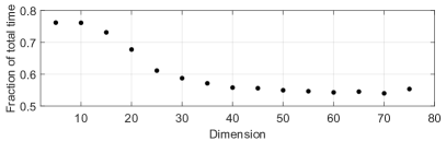
Figure 1: Time consumption by parameter tuning in relation to total execution time using 50 randomly-generated systems per dimension.

Computational Overhead

First, we investigate the computational overhead caused by the continuous adaptation of all algorithm parameters. For this purpose, we measured the time Alg. 1 spends on the adaptation and the set propagation over 50 randomly-generated systems of dimensions 5 to 75. Fig. 1 shows the fraction of the total time spent on the parameter tuning: The overhead remains manageable even for high-dimensional systems, settling at about the same time as used for the set propagation. This is achieved by the computational efficiency of Prop. 1. The overhead is more than compensated by the adaptive adjustment of the algorithm parameters as discussed at the end of this section. Also, the common practice of trial and error requires tuning times that exceed computation times by several factors.

ARCH benchmarks

Next, we have applied our algorithm to the 48-dimensional Building (BLD) benchmark and the 273-dimensional International Space Station (ISS) benchmark, both from the ARCH competition [32]. These systems are manually tuned for the competition by executing many runs to optimize the algorithm parameters with respect to the computation time while still satisfying all specifications. For a fair comparison, we set $\varepsilon_{\text{max}}{}$ to the highest possible value that still verifies the given specification. We compare our results to the tool CORA [8] since it is also implemented in MATLAB.

TABLE I: Results of ARCH benchmarks for Alg. 1 and CORA.

Benchmark	Alg. 1					CORA
	$\varepsilon_{\text{max}}{}$	Time	Steps	$[\Delta t_{\text{min}},\Delta t_{\text{max}}]$		Time	Steps	$[\Delta t_{\text{min}},\Delta t_{\text{max}}]$
BLDC01	$2\cdot 10^{-3}$	4.0s	839	$[0.0081,0.0448]$		5.5s	2400	$[0.0020,0.0100]$
BLDF01	$6\cdot 10^{-3}$	5.6s	818	$[0.0081,0.0597]$		6.0s	2400	$[0.0020,0.0100]$
ISSC01	$5.6$	21.7s	189	$[0.0704,0.1371]$		22.8s	1000	$[0.0200,0.0200]$
ISSF01	$2\cdot 10^{-3}$	295s	1216	$[0.0059,0.0395]$		849s	2000	$[0.0100,0.0100]$

Table I shows a comparison between Alg. 1 and CORA in terms of the computation time, the number of steps, and the minimum and maximum values for $\Delta t$. Alg. 1 adapts the values of the algorithm parameters depending on the current system behavior by enlarging the time step size in regions where this only moderately increases the over-approximation. The resulting range can be observed by the large differences between $\Delta t_{\text{min}}$ and $\Delta t_{\text{max}}$. Consequently, the total number of steps decreases making less computations necessary than in the case of fixed algorithm parameters as used by CORA and shown in Table I. The range for $\Delta t$ in both building benchmarks by CORA is explained by the switching between two manually-tuned time steps.

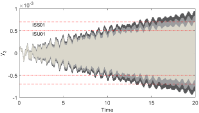
Figure 2: Benchmark ISSF01 with the specifications ISS01, ISU01, and the reachable sets $\mathcal{R}\big{(}[0,T]\big{)}$ in dark gray ($\varepsilon_{\text{max}}{}=20\cdot 10^{-3}$), light gray ($\varepsilon_{\text{max}}{}=10\cdot 10^{-3}$), and ivory ($\varepsilon_{\text{max}}{}=2\cdot 10^{-3}$).

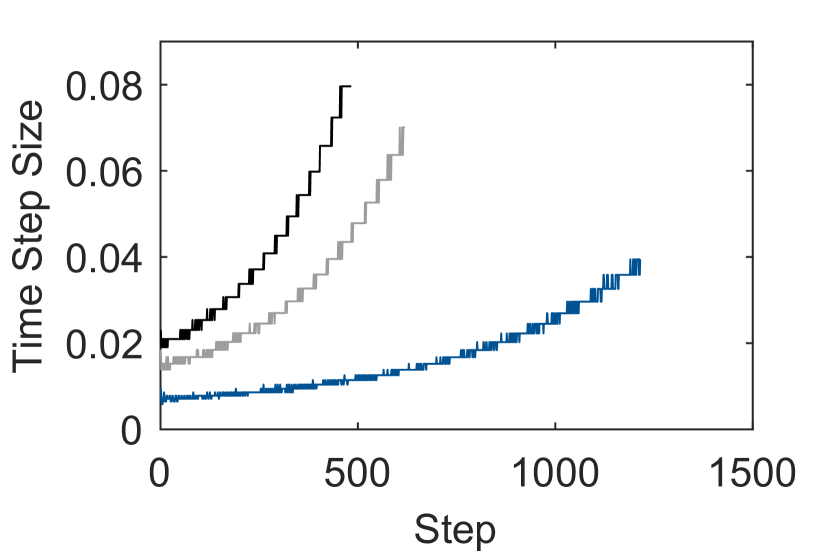
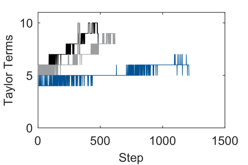
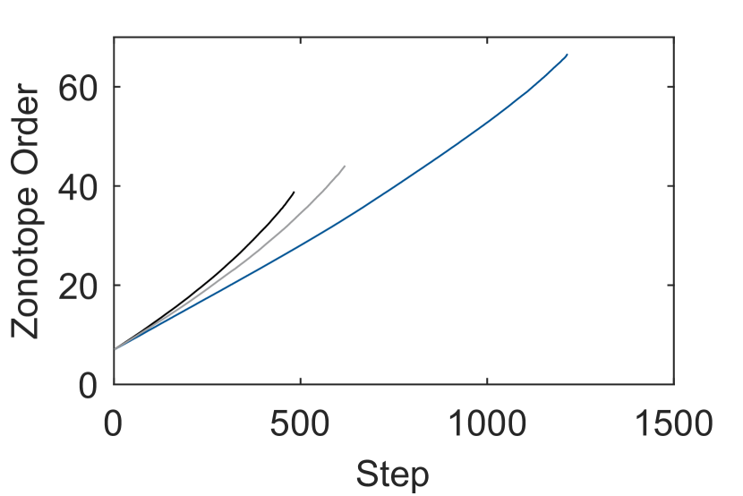
Figure 3: Benchmark ISSF01: $\Delta t,\eta,\rho{}$ for different $\varepsilon_{\text{max}}{}$: black ($\varepsilon_{\text{max}}{}=20\cdot 10^{-3}$), gray ($\varepsilon_{\text{max}}{}=10\cdot 10^{-3}$), and blue ($\varepsilon_{\text{max}}{}=2\cdot 10^{-3}$).

Fig. 2 shows the reachable sets for the benchmark ISSF01 using different values of $\varepsilon_{\text{max}}{}$: The smaller the defined error bound, the tighter are the reachable sets. We also recognize the linear increase of the admissible error bound over time as the computed sets differ more towards the end of the time horizon. Fig. 3 shows the evolution of all algorithm parameters corresponding to the different values of $\varepsilon_{\text{max}}{}$: A higher value for $\varepsilon_{\text{max}}{}$ yields a larger initial $\Delta t$ and a smaller total number of steps. Note that the switching between previously-computed values of $\Delta t$ does not add any computations since the sets are read from memory once they are computed. The number of Taylor terms $\eta$ is chosen jointly with $\Delta t$ and increases towards the end of the time horizon to facilitate larger $\Delta t$. We also observe that the zonotope order $\rho{}$ reaches a higher maximum for smaller values of $\varepsilon_{\text{max}}{}$ since in that case we cannot reduce as much as for larger $\varepsilon_{\text{max}}{}$.

Genetic Algorithm Comparison

Finally, we want to compare our approach to a genetic algorithm searching for $\Delta t$, $\eta$, and $\rho$. To this end, we use the MATLAB built-in genetic algorithm function. While the parameters $\eta$ and $\rho$ are fixed, we model the time step size by a polynomial up to order 2: $\Delta t(t)=a+bt+ct^{2}$. We restrict these parameters by the ranges $\eta\in[1,10]$, $\rho\in[2,1000]$, $a\in[0.0003,0.3],b\in[-0.1,0.1],c\in[-0.033,0.033]$. The chosen bounds for $a,b$, and $c$ restrict $\Delta t$ to suitable curves. Higher orders did not provide any benefits.

In order to establish a level playing field, we terminate once the obtained reachable set is within the box enclosure of the reachable set of the adaptive algorithm enlarged by 10%. For computational efficiency interval over-approximations were used for this comparison. The cost function is chosen as by the maximum distance to the enlarged adaptive reachable set over all dimensions.

The parameters specific to the genetic algorithm have been set as follows: We enable an infinite number of generations with a maximum of 3 stall generations. We aim to speed up the convergence by setting only 10 members per generation as the evaluation of a single member is costly in higher dimensions. For the members of the next generation, we use a standard crossover fraction of 0.75 and set the elite count to 1, carrying the best solution over to the next generation.

We applied Alg. 1 and the genetic algorithm on 50 randomly-generated systems per dimension. Table II compares the average computation time over varying dimensions of Alg. 1 to the time the genetic algorithms takes until convergence. The results show that Alg. 1 outspeeds all genetic algorithms. Since Alg. 1 tunes the algorithm parameters during runtime, we only need a single iteration for the computation of the reachable set. Contrary, the genetic algorithms run over many generations repeatedly computing the reachable set while iteratively improving the solution by means of the cost function. This process is far more time-consuming than the overhead caused by the adaptive parameter tuning. The genetic algorithm using the constant polynomial for $\Delta t$ is faster than the higher-order polynomials as they re-compute auxiliary reachable sets due to the non-constant time step size.

TABLE II: Computation time for Alg. 1 and the genetic algorithm (GA) averaged over 50 randomly-generated systems per dimension.

	Dimension
	5	10	15	20	25	30	40
Alg. 1	0.14s	0.22s	0.40s	0.58s	1.0s	1.9s	6.7s
GA (order: 0)	1.6s	3.4s	7.0s	10s	20s	30s	50s
GA (order: 1)	4.1s	9.4s	13s	21s	28s	40s	70s
GA (order: 2)	5.1s	10s	14s	21s	42s	58s	97s

Discussion

Our framework can also be applied to other computations of reachable sets and other set representations. In order to guarantee convergence and termination for all $\varepsilon_{\text{max}}{}~{}\in~{}\mathbb{R}$, Theorem 1 has to hold for the applied error terms, similarly to Sec. IV-B for the presented implementation: A tool developer has to modify $\Phi_{\text{prop,max}}{}$ and $\Phi_{\text{set}}{}$ which are, e.g., the number of template directions when using template polyhedra. An corresponding error term for the set representation has to be defined.

The choice of $\texttt{err}\big{(}\cdot\big{)}$ in (5) does not add much over-approximation as can be observed from comparing the ranges for the time step size $[\Delta t_{\text{min}},\Delta t_{\text{max}}]$ with the manually-tuned $\Delta t$ by CORA in Table I, we see that Alg. 1 chooses a similar time step size, yielding comparable results both in terms of the tightness and the computational efficiency.

The only remaining parameter for the practitioner to set is the error $\varepsilon_{\text{max}}{}$. As shown in Fig. 2, increasing the value of $\varepsilon_{\text{max}}{}$ results in a more over-approximative reachable set and vice versa. Thus, the setting of $\varepsilon_{\text{max}}{}$ is intuitive and can easily be adjusted for any system.

VI Conclusion

In this paper, we presented a novel generic framework to automatically tune all algorithm parameters which is a major problem of present reachability algorithms. The presented algorithm enables a fully-automated computation of the reachable set whose error is below a user-defined error. Previous work only considered the tuning of time parameters. An example implementation has shown to outperform manually-tuned algorithm parameters on benchmarks and provides better results than genetic algorithms searching for algorithm parameters on randomly-generated systems of varying dimensions. The extension of the presented framework to nonlinear systems will be considered in the future.

VII Acknowledgments

The authors gratefully acknowledge partial financial supports from the research training group CONVEY funded by the German Research Foundation under grant GRK 2428.

References

• [1] G. Lafferriere and et al., “Symbolic reachability computation for families of linear vector fields,” Journal of Symbolic Computation, vol. 32, no. 3, pp. 231–253, 2001.
• [2] M. Althoff and et al., “Reachability analysis of linear systems with uncertain parameters and inputs,” in Proc. of the 46th IEEE Conference on Decision and Control, pp. 726–732, 2007.
• [3] X. Chen, Reachability Analysis of Non-Linear Hybrid Systems using Taylor Models. PhD thesis, Fachgruppe Informatik, RWTH Aachen University, 2015.
• [4] A. Gurung and et al., “Parallel reachability analysis of hybrid systems in XSpeed,” International Journal on Software Tools for Technology Transfer, vol. 21, no. 4, pp. 401–423, 2019.
• [5] A. Girard and et al., “Efficient computation of reachable sets of linear time-invariant systems with inputs,” in Hybrid Systems: Computation and Control, LNCS 3927, pp. 257–271, Springer, 2006.
• [6] S. Bogomolov and et al., “Reach set approximation through decomposition with low-dimensional sets and high-dimensional matrices,” in Proc. of the 21st International Conference on Hybrid Systems: Computation and Control, pp. 41–50, 2018.
• [7] G. Frehse and et al., “SpaceEx: Scalable verification of hybrid systems,” in International Conference on Computer Aided Verification, pp. 379–395, Springer, 2011.
• [8] M. Althoff, “An introduction to CORA 2015,” in Proc. of the Workshop on Applied Verification for Continuous and Hybrid Systems, pp. 120–151, 2015.
• [9] X. Chen and et al., “Flow*: An analyzer for non-linear hybrid systems,” in International Conference on Computer Aided Verification, pp. 258–263, Springer, 2013.
• [10] R. Ray and et al., “XSpeed: Accelerating reachability analysis on multi-core processors,” in Haifa Verification Conference, pp. 3–18, Springer, 2015.
• [11] S. Bogomolov and et al., “JuliaReach: a toolbox for set-based reachability,” in Proc. of the 22nd International Conference on Hybrid Systems: Computation and Control, pp. 39–44, ACM, 2019.
• [12] S. Bak and P. S. Duggirala, “Simulation-equivalent reachability of large linear systems with inputs,” in Proc. of International Conference on Computer Aided Verification, pp. 401–420, 2017.
• [13] P. S. Duggirala and M. Viswanathan, “Parsimonious, simulation based verification of linear systems,” in Proc. of International Conference on Computer Aided Verification, pp. 477–494, 2016.
• [14] S. Bak and P. S. Duggirala, “HyLAA: A tool for computing simulation-equivalent reachability for linear systems,” in Proc. of the 20th International Conference on Hybrid Systems: Computation and Control, pp. 173–178, 2017.
• [15] A. B. Kurzhanski and P. Varaiya, “Ellipsoidal techniques for reachability analysis,” in Hybrid Systems: Computation and Control, LNCS 1790, pp. 202–214, Springer, 2000.
• [16] E. Asarin and et al., “Approximate reachability analysis of piecewise-linear dynamical systems,” in Hybrid Systems: Computation and Control, pp. 20–31, Springer, 2000.
• [17] A. Girard and C. Le Guernic, “Efficient reachability analysis for linear systems using support functions,” in Proc. of the 17th IFAC World Congress, pp. 8966–8971, 2008.
• [18] J. K. Scott and et al., “Constrained zonotopes: A new tool for set-based estimation and fault detection,” Automatica, vol. 69, pp. 126–136, 2016.
• [19] L. Lapidus and J. H. Seinfeld, Numerical solution of ordinary differential equations. Academic press, 1971.
• [20] U. M. Ascher and et al., Numerical solution of boundary value problems for ordinary differential equations. SIAM, 1994.
• [21] M. Kerbl, “Stepsize strategies for inclusion algorithms for ODE’s,” Computer Arithmetic, Scientific Computation, and Mathematical Modelling, IMACS Annals on Computing and Appl. Math, vol. 12, pp. 437–452, 1991.
• [22] W. Rufeger and E. Adams, “A step size control for Lohner’s enclosure algorithm for ordinary differential equations with initial conditions,” in Mathematics in Science and Engineering, vol. 189, pp. 283–299, Elsevier, 1993.
• [23] N. S. Nedialkov, Computing rigorous bounds on the solution of an initial value problem for an ordinary differential equation. Dissertation, University of Toronto, 2000.
• [24] P. Prabhakar and M. Viswanathan, “A dynamic algorithm for approximate flow computations,” in Proc. of the 14th International Conference on Hybrid Systems: Computation and Control, pp. 133–142, ACM, 2011.
• [25] M. Althoff, Reachability Analysis and its Application to the Safety Assessment of Autonomous Cars. Dissertation, Technische Universität München, 2010.
• [26] C. Le Guernic, Reachability analysis of hybrid systems with linear continuous dynamics. PhD thesis, Université Grenoble 1 - Joseph Fourier, 2009.
• [27] A. Girard, “Reachability of uncertain linear systems using zonotopes,” in Hybrid Systems: Computation and Control, LNCS 3414, pp. 291–305, Springer, 2005.
• [28] M. Althoff and et al., “Reachable set computation for uncertain time-varying linear systems,” in Hybrid Systems: Computation and Control, pp. 93–102, 2011.
• [29] T. A. Bickart, “Matrix exponential: Approximation by truncated power series,” Proceedings of the IEEE, vol. 56, no. 5, pp. 872–873, 1968.
• [30] M. Althoff and G. Frehse, “Combining zonotopes and support functions for efficient reachability analysis of linear systems,” in Proc. of the 55th IEEE Conference on Decision and Control, pp. 7439–7446, 2016.
• [31] A.-K. Kopetzki and et al., “Methods for order reduction of zonotopes,” in Proc. of the 56th IEEE Conference on Decision and Control, pp. 5626–5633, 2017.
• [32] M. Althoff and et al., “ARCH-COMP19 category report: Continuous and hybrid systems with linear continuous dynamics,” in Proc. of the 6th International Workshop on Applied Verification of Continuous and Hybrid Systems, pp. 14–40, 2019.