Bandit algorithms: Letting go of logarithmic regret for statistical robustness

Abstract

We study regret minimization in a stochastic multi-armed bandit setting, and establish a fundamental trade-off between the regret suffered under an algorithm, and its statistical robustness. Considering broad classes of underlying arms’ distributions, we show that bandit learning algorithms with logarithmic regret are always inconsistent, and that consistent learning algorithms always suffer a super-logarithmic regret. This result highlights the inevitable statistical fragility of all ‘logarithmic regret’ bandit algorithms available in the literature—for instance, if a UCB algorithm designed for $\sigma$-subGaussian distributions is used in a subGaussian setting with a mismatched variance parameter, the learning performance could be inconsistent. Next, we show a positive result: statistically robust and consistent learning performance is attainable if we allow the regret to be slightly worse than logarithmic. Specifically, we propose three classes of distribution oblivious algorithms that achieve an asymptotic regret that is arbitrarily close to logarithmic.

1 Introduction

The stochastic multi-armed bandit (MAB) problem seeks to identify the best among an available basket of options (a.k.a., arms), each characterized by an unknown probability distribution. Classically, these probability distribution represent rewards, and the best arm is defined as the one associated with the largest average reward. The learning algorithm, which chooses (a.k.a., pulls) one arm per decision epoch, identifies the best arm via experimentation—each pull of an arm yields one sample from the underlying reward distribution. One classical performance metric is regret, which evaluates an algorithm based on how often it pulls sub-optimal arms.

The standard approach towards algorithm design for regret minimization is as follows. First, it is assumed that the arm reward distributions belong to a specific parametric class—for example, the class of bounded distributions with support contained in $[0,b],$ or the class of $\sigma$-subGaussians. Next, algorithms are proposed for such specific parametric distribution classes, often making explicit use of the parameters (such as $b$ or $\sigma$) corresponding to the parametric distribution class. Finally, logarithmic regret guarantees are proved for such algorithms, by utilising exponential concentration inequalities (such as Hoeffding’s inequality or sub-Gaussian concentration) for that parametric distribution class.

For distribution classes such as $\sigma$-subGaussians, a logarithmic regret guarantee may not be so surprising, because such distributions enjoy exponential concentration bounds. On the other hand, when dealing with heavy-tailed arms’ distributions, it is not clear that a logarithmic regret is achievable. This is because heavy-tailed distributions (such as Pareto) are characterised by a high degree of variability, and their empirical mean estimators do not enjoy exponential concentration in the sample size. Somewhat surprisingly, a logarithmic regret guarantee was shown to be attainable in Bubeck et al. [2013] using a truncated mean estimator, for distributions satisfying a bounded moment condition. While this approach Bubeck et al. [2013] can handle heavy-tailed as well as light-tailed distributions, the algorithm still needs to know the moment bounds.

As such, a logarithmic regret guarantee has been shown to hold in a broad range of stochastic bandit settings. At this point, it is perhaps not an exaggeration to suggest that a logarithmic regret is regarded as a ‘default performance expectation’ from ‘good’ stochastic bandit learning algorithms. The present paper challenges this perceived sanctity of logarithmic regret, in the context of low-regret learning of stochastic MABs. We show that bandit algorithms that enjoy a logarithmic regret guarantee cannot be statistically robust.

Our contributions: We make two key contributions in this paper.

First, we show that bandit algorithms that enjoy a logarithmic regret guarantee are fundamentally fragile from a statistical standpoint. Equivalently, we show that statistically robust algorithms necessarily incur super-logarithmic regret. Here, an algorithm is said to be statistically robust if it exhibits consistency, i.e., the regret scales slower than any power-law, over a suitably broad class of MAB instances.

For example, consider an algorithm with logarithmic regret designed for $\sigma$-subGaussian arms. When this algorithm is used in a ‘mismatched’ bandit instance, say with $\sigma^{\prime}$-subGaussian arms ($\sigma^{\prime}>\sigma$), the learning performance can be inconsistent. That is, the regret suffered by the algorithm in the mismatched instance could have a power-law scaling in the time horizon. This is of practical concern, since the parameters that define the space of arms’ distributions (usually in the form of support/moment bounds) are often themselves estimated from limited data samples, and are therefore prone to errors.

Our second contribution is a positive result: we show that statistically robust learning is achievable if we are willing to tolerate a ‘slightly-worse-than-logarithmic’ regret in the time horizon. Specifically, we propose three classes of algorithms that (i) are distribution oblivious (i.e., they require no prior information about the arm distribution parameters), and (ii) incur a regret that is slightly super-logarithmic. The first algorithm class offers this guarantee over subexponential (a.k.a., light-tailed) instances. The latter two are designed to work robustly for general distribution instances (excepting some pathological ones).

In all three algorithms, the asymptotic regret guarantee is controlled by a certain slow-growing scaling function that is used to to define confidence bounds. A more slowly growing scaling function makes the regret asymptotically closer to logarithmic, but at the expense of a potential degradation in performance for shorter horizons. Furthermore, the regret for shorter horizon-lengths can be improved by incorporating (noisy) prior information about the reward distributions into the scaling function, without compromising on statistical robustness.

Related literature: There is a vast literature on the regret minimization for the stochastic MAB problem; we refer the reader to the textbook treatments Bubeck and Cesa-Bianchi [2012], Lattimore and Szepesvári [2018]. However, to the best of our knowledge, the issue of statistical robustness and its connection to logarithmic regret has not been explored before.

We are aware of only two other works that address statistical robustness in context of bandit algorithms, both of which consider the fixed budget pure exploration setting. For the best arm identification problem, stastistically robust algorithms have been demonstrated recently in Kagrecha et al. [2019]. For thresholding bandit problem, the algorithm proposed in Locatelli et al. [2016] is distribution-free, i.e., the algorithm does not require knowledge of the $\sigma$ parameter defining the space of $\sigma$-subGaussian rewards.

The remainder of this paper is organized as follows. We introduce some preliminaries and define the MAB formulation in Section 2. The trade-off between statistical robustness and logarithmic regret is established in Section 3. Our statistically robust algorithms and their performance guarantees are presented in Section 4, and we report the results of some numerical experiments in Section 5. An appendix, containing proofs of stated results, as well as details omitted from the main body of the paper due to space constraints, is uploaded separately as the ‘supplementary material’ document.

2 Model and Preliminaries

In this section, we introduce some preliminaries and formally define the MAB formulation.

2.1 Preliminaries

We begin by introducing the classes of reward distributions we will work with in this paper.

• $\mathcal{B}([a,b])$ denotes the set of bounded distributions with support contained in $[a,b]$. The set of all bounded distributions is denoted by $\mathcal{B}.$

• We use $\mathcal{SG}(\sigma),$ for $\sigma>0,$ to denote $\sigma$-subGaussian distributions, and $\mathcal{SG}$ to denote all subGaussian distributions.

• We denote $\mathcal{SE}(v,\alpha),$ for $v,\alpha>0,$ to denote the following class of subexponential distributions:

  $$\mathcal{SE}(v,\alpha)=\left\{F:\int e^{\lambda(x-\mu(F))}dF(x)\leq e^{\frac{v^{2}\lambda^{2}}{2}}\text{ for all }|\lambda|<\frac{1}{\alpha}\right\},$$

  where $\mu(F)$ denotes the mean of $F.$ The class of all subexponential distributions is denoted by $\mathcal{SE}.$ Distributions in $\mathcal{SE}$ are also commonly referred to as light-tailed, and those not in $\mathcal{SE}$ are called heavy-tailed (see Foss et al. [2011]).

• For $\epsilon,B>0,$ let $\mathcal{G}(\epsilon,B)$ denote the set of distributions whose $(1+\epsilon)^{th}$ absolute moment is upper bounded by $B$, i.e.,

  $$\mathcal{G}(\epsilon,B)=\left\{F:\ \int|x|^{1+\epsilon}dF(x)\leq B\right\}.$$

  In the MAB literature, $\mathcal{G}(\epsilon,B)$ is often used as the class of reward distributions in order to allow for heavy-tailed rewards (see, for example, Bubeck et al. [2013], Yu et al. [2018]). Finally, the union of the sets $\mathcal{G}(\epsilon,B)$ over $\epsilon,B>0$ is denoted by $\mathcal{G}:$

  $$\mathcal{G}=\left\{F:\ \int|x|^{1+\epsilon}dF(x)<\infty\text{ for some }\epsilon>0\right\}.$$

  $\mathcal{G}$ is the most general space of reward distributions one can work with in the context of the MAB problem—it contains all light-tailed distributions and most heavy-tailed distributions of interest.

Note that $\mathcal{B}\subset\mathcal{SG}\subset\mathcal{SE}\subset\mathcal{G}.$ We also recall the Kullback-Leibler divergence (or relative entropy) between distributions $F$ and $F^{\prime}$:

$$D(F,F^{\prime})=\int\log\left(\frac{dF(x)}{dF^{\prime}(x)}\right)dF(x),$$

where $F$ is absolutely continuous with respect to $F^{\prime}.$

Much of the vast literature on MAB problems assumes that the reward distributions lie in specific parametric subsets of $\mathcal{B},$ $\mathcal{SG},$ $\mathcal{SE},$ or $\mathcal{G};$ for example $\mathcal{B}([0,1]),$ $\mathcal{SG}(1),$ $\mathcal{G}(1,B)$ etc. Further, the parameter(s) corresponding to these subsets are ‘baked’ into the algorithms. While this approach guarantees strong performance over the parametric distribution subset under consideration (logarithmic regret, in the classical regret minimization framework), it is highly fragile to uncertainty in these parameters. Indeed, as we demonstrate in Section 3, any algorithm that enjoys logarithmic regret for a parametric subset of a distribution class must be inconsistent over the entire distribution class—specifically, when there is a parameter mismatch, the regret suffered could have a power-law scaling in the time horizon. In Section 4, we propose bandit algorithms that are statistically robust, but incur (slightly) superlogarithmic regret.

2.2 Problem formulation

Consider a multi-armed bandit (MAB) problem with $k$ arms. Let $\mathcal{M}$ be a distribution class (such as $\mathcal{B},\mathcal{SG}$ etc.) An instance $\nu=(\nu_{i},\ 1\leq i\leq k)$ of the MAB problem is defined as an element of $\mathcal{M}^{k},$ where $\nu_{i}\in\mathcal{M}$ is the distribution corresponding to arm $i$. Let $\mu_{i}$ denote the mean reward associated with arm $i,$ i.e., $\mu_{i}$ is the expected value of a random variable distributed according to $\nu_{i}.$ An optimal arm is an arm that maximizes the mean reward, i.e., one whose mean reward equals $\mu^{*}=\max_{1\leq i\leq k}\mu_{i}.$ The sub-optimality gap associated with arm $i$ is defined as $\Delta_{i}:=\mu^{*}-\mu_{i}.$

In this paper, our goal is to minimize regret. Formally, under the a policy (a.k.a., algorithm) $\pi,$ let $T_{i}(n)$ denote the number of times $i^{th}$ arm has been pulled after $n$ rounds. The regret $R_{n}(\pi,\nu)$ associated with the policy $\pi$ after $n$ rounds is defined as

$$R_{n}(\pi,\nu)=\sum_{i=1}^{n}\Delta_{i}\mathbb{E}\left[T_{i}(n)\right].$$

An algorithm is said to be consistent over $\mathcal{M}^{k}$ if, for all instances $\nu\in\mathcal{M}^{k},$ the regret satisfies $R_{n}(\pi,\nu)=o(n^{a})$ for all $a>0$ (see Lattimore and Szepesvári [2018]). For example, an algorithm that guarantees polylogarithmic regret over all instances in $\mathcal{M}^{k}$ is consistent over $\mathcal{M}^{k}.$ On the other hand, if an algorithm suffers $O(n^{a})$ regret for some $a>0$ and some instance in $\mathcal{M}^{k},$ then the algorithm is inconsistent over $\mathcal{M}^{k}.$

3 Impossibility of logarithmic regret for statistically robust algorithms

In this section, we shed light on a fundamental conflict between logarithmic regret and statistical robustness. Recall that in classical MAB formulations, it is assumed that arm reward distributions lie in, say $\mathcal{B}([0,b])$ or $\mathcal{SG}(\sigma).$ In such cases, algorithms that exploit this parametric information (i.e., the value of $b$ in the former case and the value of $\sigma$ in the latter) are known that achieve $O(\log(n))$ regret, where $n$ denotes the horizon. The celebrated UCB family of algorithms is a classic example [Lattimore and Szepesvári, 2018]. In this section, we ask the question: Are these algorithms robust with respect to the parametric information ‘baked’ into them? Our main result of this section answers this question in the negative. Specifically, we show that statistically robust algorithms (i.e., algorithms that maintain consistency over an entire class of distributions) necessarily incur super-logarithmic regret. In other words, algorithms that enjoy a logarithmic regret guarantee over a particular parametric sub-class of reward distributions are not statistically robust.

Theorem 1.

Let $\mathcal{M}\in\{\mathcal{B},\mathcal{SG},\mathcal{SE},\mathcal{G}\}.$ For any algorithm $\pi$ that is consistent over $\mathcal{M}^{k},$ and any instance $\nu\in\mathcal{M}^{k},$

$$\lim_{n\to\infty}\frac{R_{n}(\pi,\nu)}{\log(n)}=\infty.$$

The proof of Theorem 1 is provided in Appendix A. The crux of the argument is as follows. Given an MAB instance $\nu\in\mathcal{M}^{k},$ the expected number of pulls $\mathbb{E}\left[T_{i}(n)\right]$ of any suboptimal arm $i$ over a horizon of $n$ pulls, under any algorithm that is consistent over $\mathcal{M}^{k},$ is lower bounded as

$$\liminf_{n\rightarrow\infty}\frac{\mathbb{E}\left[T_{i}(n)\right]}{\log(n)}\geq\frac{1}{d_{i}},$$

where $d_{i}=\inf_{\nu^{\prime}_{i}\in\mathcal{M}}\{D(\nu_{i},\nu^{\prime}_{i}):\ \mu(\nu^{\prime}_{i})>\mu^{*}(\nu)\}$ (see Lattimore and Szepesvári [2018, chap. 16]). Informally, $d_{i}$ is the smallest perturbation of $\nu_{i}$ in relative entropy sense that would make arm $i$ optimal. The proof of Theorem 1 follows by showing that when $\mathcal{M}$ is $\mathcal{B},$ $\mathcal{SG},$ $\mathcal{SE}$ or $\mathcal{G},$ we have $d_{i}=0$ for all suboptimal arm of any instance. In other words, given any distribution $\eta\in\mathcal{M},$ there exists another distribution $\eta^{\prime}\in\mathcal{M}$ such that $\mu(\eta^{\prime})$ is arbitrarily large, even while $D(\eta,\eta^{\prime})$ is arbitrarily small.

Theorem 1 highlights that classical bandit algorithms are not robust with respect to uncertainty in support/moment bounds. For example, consider any algorithm $\pi$ that guarantees logarithmic regret over $\mathcal{SG}(1)$ (for example, the algorithms presented in Chapters 7–9 in Lattimore and Szepesvári [2018]). Theorem 1 implies that all such algorithms are inconsistent over $\mathcal{SG}.$ This reveals an inherent fragility of such algorithms—while they might guarantee good performance over the specific parametric sub-class of reward distributions they are designed for, they are not robust to uncertainty with respect to the parameters that specify the distribution class.

Having shown that robust algorithms cannot achieve logarithmic regret, in the following section, we present statistically robust algorithms for $\mathcal{SE},$ and $\mathcal{G}.$ (Of course, an algorithm that is robust over $\mathcal{SE}$ is also robust over $\mathcal{B}$ and $\mathcal{SG}$). Specifically, these algorithms attain a regret that is slightly superlogarithmic, while remaining consistent over $\mathcal{SE}$ and $\mathcal{G}$ respectively.

4 Statistically robust algorithms

In this section, we demonstrate how statistical robustness can be achieved by allowing for slightly superlogarithmic regret. In particular, we propose algorithms that are distribution oblivious, i.e., they do not require any prior information about the arm distributions in the form of support/moment/tail bounds. By suitably choosing a certain scaling function that paramterizes the algorithms, the associated regret can be made arbitrarily close to logarithmic (in the time horizon). However, this is not an entirely ‘free lunch’—tuning the scaling function for stronger asymptotic regret guarantees can affect the regret for moderate horizon values. Interestingly though, this trade-off between asymptotic and short-horizon performance can be tempered by incorporating (noisy) prior information about support/moment bounds on the arm distributions into the scaling functions, while maintaining statistical robustness.

We propose three distribution oblivious algorithms for robust regret minimization in this section. The first, which we call Robust Upper Confidence Bound (R-UCB) algorithm is suitable for subexponential (light-tailed) instances. (An instance is said to be light-tailed if all arm distributions are light-tailed). It uses the empirical average as an estimator for the mean reward, and uses a confidence bound that that is a suitably (and robustly) scaled version of the typical non-oblivious confidence bounds in UCB algorithms.

Next, to deal with the most general class $\mathcal{G}$ of reward distributions, we propose another algorithm, called R-UCB-G, which uses truncated mean estimators. Empirical averages, which provide good estimates of the mean for light-tailed arms, can deviate significantly from the true mean for heavy-tailed arms. To control the ‘high variability’ in the sample values, a truncated mean estimator is typically used; see for example, Bubeck et al. [2013], Yu et al. [2018]. The truncation parameter in R-UCB-G is scaled with time suitably to provide statistical robustness. Desirably, both R-UCB & R-UCB-G are anytime algorithms, and have provable regret guarantees.

Another technique for mean estimation that works well under excessive variability in the sample values is the Median of Means approach [Bubeck et al., 2013]. We design a statistically robust anytime algorithm over $\mathcal{G}^{k}$ using this approach; due to space constraints, the algorithm and its performance characterization are presented in Appendix D.

Before we describe the algorithms, we define the following class of functions which serve as scaling functions for both algorithms.

Definition 1.

A function $f:\mathbb{N}\rightarrow(0,\infty)$ is said to be slow growing if

$$f(t+1)\geq f(t)\ \forall\ t\in\mathbb{N},\quad\lim_{t\rightarrow\infty}f(t)=\infty,\quad\lim_{t\rightarrow\infty}\frac{f(t)}{t^{a}}=0\ \forall\ a>0.$$

4.1 Robust Upper Confidence Bound algorithm for light-tailed instances

Algorithm 1 R-UCB

Input $k$ arms, slow growing scaling function $f$

for $t=1$ to $k$ do

     Pull arm with index $i=t-1$ and observe reward $R_{t}$

     Update $\hat{\mu}(i,u_{i})\leftarrow r$, $u_{i}\leftarrow 1$

end for

for  $t=k+1,k+2,\dots$  do

     Calculate the upper confidence bound as

$$\mathcal{U}(i,u_{i},t)=\hat{\mu}(i,u_{i})+\underbrace{\sqrt{\frac{f(t)\log(t)}{u_{i}}}}_{\mathcal{W}(u_{i},t)}$$

     Pull arm $i$ maximizing $\mathcal{U}(i,u_{i},t)$ and observe reward $R_{t}$

     Update empirical average $\hat{\mu}(i,u_{i})$ and $u_{i}\leftarrow u_{i}+1$

end for

The R-UCB algorithm is presented in Algorithm 1. The only structural difference between R-UCB and the classical UCB algorithm is in the definition of the upper confidence bound—under R-UCB, the confidence width $\mathcal{W}(u_{i},t)$ for arm $i$ at time $t,$ where $u_{i}$ denotes the number of pulls of arm $i$ prior to time $t,$ is scaled by a slow growing function $f.$ This simple scaling provides statistical robustness over light-tailed instances, as established in Theorem 2 below. We prove the consistency of R-UCB over all subexponential instances, albeit with superlogarithmic regret. We also provide stronger guarantees for subgaussian instances.

Theorem 2.

Consider the algorithm R-UCB with a specified slow growing scaling function $f.$ For an instance $\nu\in\mathcal{SE}(v,\alpha)^{k},$ there exists threshold $t^{\mathcal{SE}}_{min}(v,\alpha)$ such that for $t>t^{\mathcal{SE}}_{min}(v,\alpha),$ the regret under R-UCB satisfies

$$R_{t}(\nu)\leq\sum_{i:\Delta_{i}>0}\left(f(t)\log(t)~{}\max\left\{\frac{4}{\Delta_{i}},\Delta_{i}\left(\frac{\alpha}{v^{2}}\right)^{2}\right\}+4\Delta_{i}\right).$$ (1)

For an instance $\nu\in\mathcal{SG}(\sigma)^{k},$ there exists a threshold $t^{\mathcal{SG}}_{min}(\sigma)$ such that for $t>t^{\mathcal{SG}}_{min}(\sigma),$ the regret under R-UCB satisfies

$$R_{t}(\nu)\leq\sum_{i:\Delta_{i}>0}\left(\frac{4f(t)\log(t)}{\Delta_{i}}+4\Delta_{i}\right).$$ (2)

The key take-aways from Theorem 2 are as follows.

• R-UCB is clearly consistent over $\mathcal{SE}^{k},$ but the regret guarantee is super-logarithmic, as demanded by Theorem 1.

• R-UCB is distribution oblivious in the sense that it does not need the parameters $v,\alpha$ in the implementation. However, the stated regret guarantee holds for $t$ greater than an instance-dependent threshold $t^{\mathcal{SE}}_{min}(v,\alpha)$—this is because the confidence width needs to be large enough for certain concentration properties to hold. Explicit characterization of the threshold $t^{\mathcal{SE}}_{min}(v,\alpha)$, along with (weaker) regret bounds for $t$ less than this threshold, are provided in Appendix B.

• Choosing $f$ to be ‘slower’ growing leads to better asymptotic regret guarantees, but increases the threshold $t_{min}.$ This implies a trade-off between asymptotic and short-horizon performance in a purely oblivious setting. However, (noisy) prior information about the class of arm distributions can be incorporated into the choice of scaling function $f$ to dilute this tradeoff. For example, if it is believed that the arm distributions are $\sigma$-subgaussian, then one may set $f(t)=8\sigma^{2}+h(t),$ where $h(\cdot)$ is slow growing; this choice of motivated by the observation that for the well known (non-robust) $\alpha$-UCB algorithm [Bubeck and Cesa-Bianchi, 2012], $f$ would be replaced by $2\alpha\sigma^{2},$ $\alpha>1$ for $\sigma$-subGaussian arms. This choice would make $t^{\mathcal{SG}}_{min}$ small if the arms are $\sigma^{\prime}$-subgaussian, where $\sigma^{\prime}\approx\sigma,$ while still providing statistical robustness to the reliability of this prior information; see Appendix B. We also illustrate this phenomenon in our numerical experiments in Section 5.

• Stronger performance guarantees are possible for the subclass $\mathcal{SG}^{k}.$ Indeed, given that $\mathcal{SG}(\sigma)\subset\mathcal{SE}(\sigma,\alpha)$ for all $\alpha>0,$ the guarantee (2) is stronger than (1) for $\nu\in\mathcal{SG}(\sigma)^{k}.$

The proof of Theorem 2 is provided in Appendix B.

4.2 Robust Upper Confidence Bound algorithm for arbitrary instances

The R-UCB algorithm discussed above is robust to parametric uncertainties, and guarantees ‘slightly-worse-than-logarithmic’ regret for any light-tailed bandit instance. However, one could argue that R-UCB is still not truly robust—after all, how can we be certain in a practical scenario that there are no heavy-tailed arms involved? From a viewpoint of applications such as financial portfolios and insurance, heavy-tailed distributions are ubiquitously used in modelling. Therefore there is a compelling case for handling heavy-tailed as well as light-tailed arms’ distributions within a common, statistically robust framework.

In this section, we propose a truly robust algorithm for the most general setting, i.e., for bandit instances in $\mathcal{G}^{k}.$ We recall that the class $\mathcal{G}$ demands only the boundedness of the $(1+\epsilon)$-moment for some $\epsilon>0.$ This is only mildly more demanding than the finiteness of the mean, which is necessary for the MAB problem to be well-posed.

Once the restriction to light-tailed reward distributions is removed, more sophisticated estimators than empirical averages are required; this is because empirical averages are highly sensitive to (relatively frequent) outliers in heavy-tailed data. One such approach is to use truncation-based estimators (see, for example, Bubeck et al. [2013]), which offer lower variability at the expense of a (controllable) bias. The R-UCB-G algorithm, stated formally as Algorithm 2, uses a truncation-based estimator in conjunction with a robust scaling of the confidence bound. Note that the same scaling function $f$ is used for both truncation as well for scaling the confidence bound.

R-UCB-G provides the following performance guarantee over instances in $\mathcal{G}^{k}.$ To the best of our knowledge, this is the first time a single algorithm has been shown to provide provable regret guarantees in such generality.

Algorithm 2 R-UCB-G

Input $k$ arms, slow growing scaling function $f$ taking values in $(1,\infty)$

Initialize $\mathcal{R}_{i}=\{~{}\}$, $u_{i}=0$ for all arm $i$

for $t=1$ to $k$ do

     pull arm with index $i=t-1$ and observe reward $r$

     Append r to $\mathcal{R}_{i}$ and update $u_{i}\leftarrow u_{i}+1$

end for

for  $t=k+1,k+2,\dots$  do

     Calculate the upper confidence bound as

$$\mathcal{U}(i,u_{i},t)=\underbrace{\frac{1}{u_{i}}\sum_{X\in\mathcal{R}_{i}}X\mathbbm{1}_{\left\{|X|\leq f(t)\right\}}}_{\hat{\mu}(i,u_{i},t)}+\underbrace{\frac{1}{\log(f(t))}+\frac{16f(t)\log(t)}{u_{i}}}_{\mathcal{W}(u_{i},t)}$$

     Pull arm $i$ maximizing $\mathcal{U}(i,u_{i},t)$ and observe reward $R_{t}$

     Append $R_{t}$ to $\mathcal{R}_{i}$ and update $u_{i}\leftarrow u_{i}+1$

end for

Theorem 3.

Consider the algorithm R-UCB-G with a specified slow growing scaling function $f$ taking values in $(1,\infty).$ For an instance $\nu\in\mathcal{G}(\epsilon,B)^{k},$ there exists a threshold $t_{min}(\epsilon,B)$ such that for $t>t_{min}(\epsilon,B),$ the regret under R-UCB-G satisfies

$$R_{t}(\nu)\leq\sum_{i:\Delta_{i}>0}\left(\frac{32f(t)\log(t)}{1-\frac{2}{\Delta_{i}\log(f(t))}}+4\Delta_{i}\right).$$

The performance guarantee of R-UCB-G is structurally similar to that for R-UCB: The algorithm is consistent, with a super-logarithmic regret that is dictated by the growth of the scaling function $f.$ Moreover, while slowing the growth of $f$ improves the asymptotic regret guarantee, it causes $t_{min}$ to increase, potentially compromising the performance for shorter horizons. As before, prior information on, say, moment bounds satisfied by the arm distributions can be incorporated into the design of $f.$ For example, if it is believed that $\nu\in\mathcal{G}(\epsilon,B),$ a natural choice of $f$ would be $f(t)=c+h(t),$ where $h(\cdot)$ is a slow growing function, and $c>1$ is the smallest constant satisfying: $\log(x)\leq x^{\epsilon}/3B$ for all $x\geq c;$ this choice would make $t_{min}$ close to zero for instances in $\mathcal{G}(\epsilon^{\prime},B^{\prime})^{k},$ for $\epsilon^{\prime}\approx\epsilon,$ $B^{\prime}\approx B$ (see Appendix C). The proof of Theorem 3 is provided in Appendix C.

5 Experimental Analysis

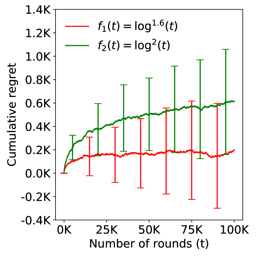
(a) R-UCB: Comparison between different scaling functions

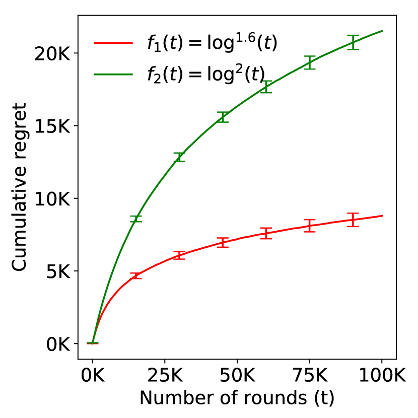
(b) R-UCB-G: Comparison between different scaling functions

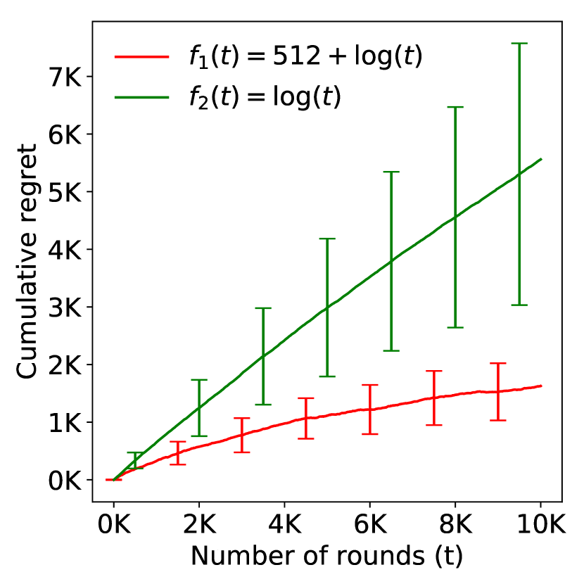
(c) Using prior information to improve short-horizon regret

In this section, we present numerical results to illustrate the performance of the algorithms presented in Section 4.

In the first experiment, we demonstrate the effect of choice of scaling function $f$ on the cumulative regret. As per Theorems 2 and 3, the regret grows faster asymptotically if we choose a faster growing $f$. We demonstrate this behavior for R-UCB and R-UCB-G in Figures 1(a) and 1(b) respectively. The chosen instance is as follows: two arms both distributed as Gaussian $\mathcal{N}(\mu,\sigma)$ with parameters $(1.7,1)$ and $(3.7,3)$. This choice of parameters is arbitrary and a similar trend was observed in trials with other Gaussian instances. The two chosen scaling functions are $f_{1}(t)=\log^{1.6}(t)$, and $f_{2}(t)=\log^{2}(t)$. The simulation is repeated 200 times for each configuration and the empirical mean is plotted along with the standard deviation in Figures 1(a) and 1(b) for R-UCB and R-UCB-G, respectively. We note that the observed cumulative regret corresponding to the faster growing $f_{2}(t)$ exceeds that corresponding to $f_{1}(t)$ in both cases. Interestingly, this dominance holds even for smaller horizon values, even though our regret bounds suggests that tuning the scaling function for better asymptotic performance might compromise short-horizon regret. This is because our regret bounds (and UCB upper bounds in the literature most generally) are fairly loose. Indeed, we also observe that the cumulative regret in all the cases is well below the bounds presented in Theorems 2 and 3. Also, the regret of R-UCB is less than R-UCB-G for the same choice of $f(t),$ which is reasonble considering we have used a light-tailed instance.

In the second experiment, we demonstrate how choosing $f(t)$ based on (noisy) prior information can decrease regret over short horizons. The chosen instance for this experiment is as follows: two arms both distributed as Gaussian $\mathcal{N}(\mu,\sigma)$ with parameters $(0,1)$ and $(1,10)$. Now, suppose we have the (noisy) prior information that the arms are $\sigma$-subGaussian with $\sigma\approx 8$. As stated in Section 4, we incorporate this prior information into the design of $f(t)$ by choosing $f_{1}(t)=512+\log(t)$. We compare the cumulative regret for this choice with that corresponding to a completely oblivious choice of $f(t)$, i.e., $f_{2}(t)=\log(t)$. The experiment is repeated 200 times and obtained mean and standard deviation of regret is shown in Figure 1(c). We can see that $f_{1}(t)$, i.e., the scaling function chosen based on the prior information, incurs lower regret. This trend in cumulative regret can be reasoned as follows. The algorithm using scaling function $f_{2}(t)$ uses smaller confidence widths, which results in greater susceptibility to the noise in the arm rewards. In conclusion, if noisy prior information about the possible arm distributions is available, this can be incorporated into the choice of the scaling function to improve short-horizon performance, while retaining statistical robustness.

6 Concluding remarks

In this paper, we demonstrated the fundamental trade-off between logarithmic regret and statistical robustness in stochastic MABs. We also proposed robust algorithms that incur slightly super-logarithmic regret. It would be interesting to explore similar trade-offs between statistical robustness and performance in other bandit settings, including thresholding bandits [Locatelli et al., 2016], linear bandits [Rusmevichientong and Tsitsiklis, 2010] and combinatorial bandits [Chen et al., 2013].

More broadly, we hope that this paper spawns further work on statistically robust online learning algorithms. We have focussed on one of the simplest learning paradigms (regret minimization in MABs), where a logarithmic regret emerged as a robustly unattainable performance barrier. Other fundamental performance barriers of statistically robust learning await discovery, in more challenging settings such as Markovian bandits and Markov Decision Processes.

Broader Impact

This work does not present any foreseeable ethical or societal consequences.

Appendix A Appendix for Section 3 - Impossibility of logarithmic regret for statistically robust algorithms

This section is devoted to the proof of Theorem 1. The proof is based on the following characterization of instance-dependent lower bounds from Lattimore and Szepesvári [2018] (see Theorem 16.2):

Theorem 4.

For any algorithm $\pi$ that is consistent over $\mathcal{M}^{k},$ and instance $\nu\in\mathcal{M}^{k},$

$$\lim_{n\to\infty}\inf\frac{R_{n}(\pi,\nu)}{\log(n)}\geq\sum_{i:\Delta_{i}>0}\frac{\Delta_{i}}{d_{i}(\nu_{i},\mu^{*},\mathcal{M})},$$

where $d_{i}(\nu_{i},\mu^{*},\mathcal{M}):=\inf_{\nu^{\prime}_{i}\in\mathcal{M}}\{D(\nu_{i},\nu^{\prime}_{i}):\ \mu(\nu^{\prime}_{i})>\mu^{*}\}.$

The proof of Theorem 1 therefore follows from the following lemma, which shows that $d_{i}(\nu_{i},\mu^{*},\mathcal{M})=0$ for all suboptimal arms of any instance $\nu$ when $\mathcal{M}$ is $\mathcal{B},$ $\mathcal{SG},$ $\mathcal{SE},$ or $\mathcal{G}.$

Lemma 1.

Fix $\mathcal{M}\in\{\mathcal{B},\mathcal{SG},\mathcal{SE},\mathcal{G}\}.$ For any distribution $F\in\mathcal{M},$ and for any $a>0$ and $b>\mu(F)$, there exists distribution $F^{\prime}\in\mathcal{M}$ such that

$$D(F,F^{\prime})\leq a\quad\text{ and }\quad\mu(F^{\prime})\geq b.$$

Proof.

We consider the following two cases.

Case 1: $\mathcal{M}\in\{\mathcal{SG},\mathcal{SE},\mathcal{G}\}$

If the distribution $F$ is unbounded from above (i.e., $\bar{F}(y)>0$ for all $y\in\mathbb{R}$), then the claim follows from Lemma 1 in Agrawal et al. [2020]. The idea there is to construct a new distribution $F^{\prime}$ such that for a chosen $y$, the CDF on the left side is decreased by a factor of $e^{-a}$ with respect to $F,$ and rest of the mass is pushed on the right side of $y$. Crucially, under this perturbation, $F^{\prime}$ remains in $\mathcal{M}$, since on both sides of $y$ only a constant is being multiplied, thus keeping the functional form of the distribution same. The KL-divergence $D(F,F^{\prime})$ is always less than $a$ independent of the choice of $y$. However, the mean of $F^{\prime}$ can be made arbitrary large by choosing a suitably large value of $y$.

On the other hand, if $F$ is bounded from above, then the argument below (for the case $\mathcal{M}=\mathcal{B}$) can be applied to construct $F^{\prime}$ that is also bounded from above, but satisfies the conditions required. (Specifically, the boundedness of the lower end-point of the support is not required for this argument.)

Case 2: $\mathcal{M}=\mathcal{B}$

We construct a new bounded distribution $F^{\prime}$ such that the CDF of $F^{\prime}$ is $e^{-a}$ times the CDF of $F$ over its support. The rest of the probability mass is uniformly distributed starting from the right end-point of the support to an arbitrary point $v^{\prime}$.

Suppose that the support of $F$ is contained within $[u,v].$ Define the CDF of distribution $F^{\prime}$ as follows, for $\gamma\in(0,1)$ and $v^{\prime}>v.$

$$F^{\prime}(x) =(1-\gamma)F(x)\qquad\forall\ x\leq v$$

$$F^{\prime}(x) =1+\gamma\frac{x-v^{\prime}}{v^{\prime}-v}\qquad\forall\ x\in(v,v^{\prime}]$$

Now,

$$D(F,F^{\prime})=\int_{u}^{v}\log\left(\frac{dF(x)}{dF^{\prime}(x)}\right)dF(x)=-\log(1-\gamma).$$

Choosing $\gamma=1-e^{-a}$ yields $D(F,F^{\prime})=a$. Turning now to the mean of $F^{\prime},$

$$\mu(F^{\prime}) =\int_{u}^{v^{\prime}}xdF^{\prime}(x)=(1-\gamma)\mu(F)+\int_{v}^{v^{\prime}}x\frac{\gamma}{v^{\prime}-v}dx$$

$$=(1-\gamma)\mu(F)+\frac{\gamma}{2}(v^{\prime}+v)$$

Clearly, $\mu(F^{\prime})$ can be made arbitrarily large by choosing a suitably large $v^{\prime}.$

∎

Appendix B Proof of Theorem 2 - Regret Upper Bound for R-UCB

We formally prove theorem 2 in this section. The prove is structurally similar to the bandit regret proof presented in Bubeck, Cesa-Bianchi, and Lugosi [2013]. We will show regret bound for the two cases $\nu\in\mathcal{SG}^{k}$, and, $\nu\in\mathcal{SE}^{k}$.

Proof.

We first prove for $\nu\in\mathcal{SE}^{k}$ and then the other case follows.

Case 1    $\nu\in\mathcal{SE}^{k}$

We define the following three events for any sub-optimal arm $i$.

$$E_{1}~{} :\qquad\mathcal{U}(i^{*},T_{i^{*}}(t-1),t)\leq\mu^{*}$$

$$E_{2} :\qquad\hat{\mu}(i,T_{i}(t-1))>\mu_{i}+\mathcal{W}(T_{i}(t-1),t)$$

$$E_{3} :\qquad\Delta_{i}<2\mathcal{W}(T_{i}(t-1),t)$$

where $T_{i}(t)$ denotes the number of times $i^{th}$ arm is pulled till time instant $t$. The three events can be interpreted as follows. Event $E_{1}$ occurs when the upper confidence bound corresponding to the optimal arm is less than its actual mean. Event $E_{2}$ corresponds to the case when the mean estimator of a sub-optimal arm is much more than its actual mean. As we shall see, both $E_{1}$ and $E_{2}$ are low-probability event and its probability can be upper bounded. Finally, event $E_{3}$ corresponds to the case when the confidence window of arm $i$ is large. We now prove that one of these event must be true when a sub-optimal arm is chosen at time instant $t$. Denote $I_{t}$ as the arm chosen at time $t$.

Claim    If $I_{t}=i$, then one of $E_{1},E_{2}$ or $E_{3}$ is true.

To justify this claim, we assume all the three events to be false and then show a contradiction.

We have,

$$\mathcal{U}(i^{*},T_{i^{*}}(t-1),t) >\mu^{*}$$

$$=\mu_{i}+\Delta_{i}$$

$$\geq\mu_{i}+2\mathcal{W}(T_{i}(t-1),t)$$

$$\geq\hat{\mu}(i,T_{i}(t-1))+\mathcal{W}(T_{i}(t-1),t)$$

$$=\mathcal{U}(i,T_{i}(t-1),t)$$

which is a contradiction since $I_{t}\neq i^{*}$.

We now show a distribution oblivious concentration inequality for each $\nu\in\mathcal{SE}^{k}$. This inequality will be useful in upper bounding probability of events $E_{1}$ and $E_{2}$.

By our choice of algorithm

$$\hat{\mu}(i,u)=\frac{1}{u}\sum_{j=1}^{u}X_{j}~{}\text{;}~{}~{}~{}~{}\mathcal{W}(u,t)=\sqrt{\frac{f(t)\log(t)}{u}}$$

We assume the underlying distribution to be $\nu\in\mathcal{SE}(v,\alpha)^{k}$. For any confidence width $\mathcal{W}$, we have the following concentration inequality (see equation 2.18 in Wainwright [2019])

$$\mathbb{P}\left(\frac{1}{u}\sum_{j=1}^{u}X_{j}-\mu\geq\mathcal{W}\right)\leq\text{exp}\left(-\min\left\{\frac{u\mathcal{W}^{2}}{2v^{2}},\frac{u\mathcal{W}}{2\alpha}\right\}\right)$$

We are interested only in small values of the confidence window $\mathcal{W}$, and hence the first term in the minimum expression is of interest to us. For the first term to be less than the second term, we have the following inequality

$$\mathcal{W}\leq\frac{v^{2}}{\alpha}$$

Putting the value of confidence window $\mathcal{W}(u,t)$ in this inequality, we get,

$$u\geq f(t)\log(t)\left(\frac{\alpha}{v^{2}}\right)^{2}$$

Denote the minimum $u$ satisfying this inequality as $u_{0}$. Hence for all $u>u_{0}$ we have,

$$\mathbb{P}\left(\hat{\mu}(i^{*},u)+\mathcal{W}(u,t)>\mu^{*}\right)\leq\text{exp}\left(\frac{-f(t)\log(t)}{2v^{2}}\right)$$

Since $f(t)$ is a sub-linearly growing function, for all time $t>t_{0}$, we are guaranteed to have $f(t)>8v^{2}$, where $t_{0}=f^{-1}(8v^{2})$. Substituting this inequality in the above expression yields,

$$\mathbb{P}\left(\hat{\mu}(i^{*},u)+\mathcal{W}(u,t)>\mu^{*}\right)\leq\text{exp}\left(-4\log(t)\right)=t^{-4}$$

This expression establishes a distribution oblivious inequality for subexponential random variables. This inequality is valid for all time instances $t>t_{0}$ and $u>u_{0}$, where $t_{0}$ is a distribution dependent constant parameter while $u_{0}$ depends on the distribution as well as the choice of $f$. In addition, $u_{0}$ is an increasing function with number of rounds $t$.

This inequality is useful in establishing an upper bound on the probability of events $E_{1}$ and $E_{2}$. We have,

$$\mathbb{P}(E_{1}) \leq\mathbb{P}(\exists u\in[t]:\mathcal{U}(i^{*},u,t)\leq\mu^{*})\leq t.t^{-4}=t^{-3}~{}~{}\text{by union bound over }u$$

Similarly, $\mathbb{P}(E_{2})\leq t^{-3}$.

Let $u^{\prime}_{i}$ denote the maximum value of $T_{i}(t-1)$ for which event $E_{3}$ is true. Consequently, for all $t>u^{\prime}_{i}$ and $u>u_{0}$, if $I_{t}=i$, then at least one of the event $E_{1},$ $E_{2}$ is true. Finally, we choose $u_{i}=\max(u^{\prime}_{i},u_{0},t_{0})$ since we wish to apply the above concentration inequality for all time instances $t>u_{i}$.

Now, for any sub-optimal arm $i$,

$$\mathbb{E}[T_{i}(t)] =\mathbb{E}\left[\sum_{s=1}^{t}\mathbbm{1}\{I_{t}=i\}\right]$$

$$\leq u_{i}+\mathbb{E}\left[\sum_{s=u_{i}+1}^{t}\mathbbm{1}\{I_{t}=i\}\right]$$

$$=u_{i}+\mathbb{E}\left[\sum_{s=u_{i}+1}^{t}\mathbbm{1}\{I_{t}=i,E_{1}\text{ true or }E_{2}\text{ true}\}\right]$$

$$\leq u_{i}+\sum_{s=u_{i}+1}^{t}\mathbb{P}(E_{1}\cup E_{2})$$

$$\leq u_{i}+\sum_{s=u_{i}+1}^{t}\frac{2}{s^{3}}\leq u_{i}+4$$

Evaluating the value of $u_{i}$, we get

$$u_{i}=\max\left\{\frac{4f(t)\log(t)}{\Delta_{i}^{2}},f(t)\log(t)\left(\frac{\alpha}{v^{2}}\right)^{2},t_{0}\right\}$$

However, we observe that $t_{0}$ is a constant and thus the first two terms ($u^{\prime}_{i},u_{0}$) will be more than $t_{0}$ after a time instance, say $t_{1}$. Hence,

$$\mathbb{E}[T_{i}(t)]\leq\max\left\{\frac{4f(t)\log(t)}{\Delta_{i}^{2}},f(t)\log(t)\left(\frac{\alpha}{v^{2}}\right)^{2}\right\}+4\quad\forall t>t^{\mathcal{SE}}_{min}(\nu)$$

where the instance dependent threshold $t^{\mathcal{SE}}_{min}(\nu)=\max(t_{0},t_{1})$.

Thus, we get the regret upper bound as

$$\boxed{R_{t}(\nu)\leq\sum_{i:\Delta_{i}>0}\left(f(t)\log(t)~{}\max\left\{\frac{4}{\Delta_{i}},\Delta_{i}\left(\frac{\alpha}{v^{2}}\right)^{2}\right\}+4\Delta_{i}\right)\quad\forall t>t^{\mathcal{SE}}_{min}(\nu)}$$

Case 2    $\nu\in\mathcal{SG}^{k}$

We observe that, $\mathcal{SG}$ is a special case of $\mathcal{SE}$ with $\alpha\rightarrow 0$. And hence, the regret expression can be obtained as

$$\boxed{R_{t}(\nu)\leq\sum_{i:\Delta_{i}>0}\left(\frac{4f(t)\log(t)}{\Delta_{i}}+4\Delta_{i}\right)\quad\forall t>t^{\mathcal{SG}}_{min}(\nu)}$$

where the instance dependent threshold $t^{\mathcal{SG}}_{min}=\max(t_{0},t_{1})$ with $t_{0}$ and $t_{1}$ same as the previous case.

∎

B.1 Regret bounds when $t<t_{min}$

We discuss a weaker regret bound for time instances less than the threshold time $t_{min}$. In the proof of theorem 2 above, we use a slow increasing scaling function to make the inequality oblivious to its parameters. However, we are also interested in obtaining a regret bound for $t<t_{min}$. We have,

$$\mathbb{P}\left(\hat{\mu}(i^{*},u)+\mathcal{W}(u,t)>\mu^{*}\right)\leq\text{exp}\left(-\hat{c}f(t)\log(t)\right)$$

where

$$\hat{c}=\begin{cases}\frac{2}{(b-a)^{2}},&\text{if }\nu\in\mathcal{B}^{k}\\ \frac{1}{2\sigma^{2}},&\text{if }\nu\in\mathcal{SG}^{k}\\ \frac{1}{2v^{2}},&\text{if }\nu\in\mathcal{SE}^{k}\end{cases}$$

Substituting this weaker concentration bound in the above proof of regret bound we get,

$$\mathbb{E}[T_{i}(t)]\leq u_{i}+\sum_{s=u_{i}+1}^{t}t^{1-\hat{c}f(t)\log(t)}$$

as the expected number of times a sub-optimal arm is pulled. The above expression for $\mathbb{E}[T_{i}(t)]$ still yields a sub-linear upper bound, though weaker than before.

Appendix C Proof of Theorem 3 - Regret Upper Bound for R-UCB-G

We prove theorem 3 in this section. This proof is similar to proof of theorem 2 given in appendix B.

Proof.

We define the following three events for any sub-optimal arm $i$.

$$E_{1}~{} :\qquad\mathcal{U}(i^{*},T_{i^{*}}(t-1),t)\leq\mu^{*}$$

$$E_{2} :\qquad\hat{\mu}(i,T_{i}(t-1),t)>\mu_{i}+\mathcal{W}(T_{i}(t-1),t)$$

$$E_{3} :\qquad\Delta_{i}<2\mathcal{W}(T_{i}(t-1),t)$$

where $T_{i}(t)$ denotes the number of times $i^{th}$ arm is pulled till time instant $t$. The three events can be interpreted as follows. Event $E_{1}$ occurs when the upper confidence bound corresponding to the optimal arm is less than its actual mean. Event $E_{2}$ corresponds to the case when the mean estimator of a sub-optimal arm is much more than its actual mean. As we shall see, both $E_{1}$ and $E_{2}$ are low-probability event and its probability can be upper bounded. Finally, event $E_{3}$ corresponds to the case when the confidence window of arm $i$ is large. We now prove that one of these event must be true when a sub-optimal arm is chosen at time instant $t$. Denote $I_{t}$ as the arm chosen at time $t$.

Claim    If $I_{t}=i$, then one of $E_{1},E_{2}$ or $E_{3}$ is true.

To justify this claim, we assume all the three events to be false and then show a contradiction.

We have,

$$\mathcal{U}(i^{*},T_{i^{*}}(t-1),t) >\mu^{*}$$

$$=\mu_{i}+\Delta_{i}$$

$$\geq\mu_{i}+2\mathcal{W}(T_{i}(t-1),t)$$

$$\geq\hat{\mu}(i,T_{i}(t-1),t)+\mathcal{W}(T_{i}(t-1),t)$$

$$=\mathcal{U}(i,T_{i}(t-1),t)$$

which is a contradiction since $I_{t}\neq i^{*}$.

Now, by our choice of algorithm

$$\hat{\mu}(i,u,t)=\frac{1}{u}\sum_{j=1}^{u}X_{j}\mathbbm{1}_{\left\{|X_{j}|\leq f(t)\right\}}$$

We attempt to establish a distribution oblivious concentration inequality with mean estimator chosen as $\hat{\mu}(i,u,t)$. We draw inspiration from already established non-oblivious concentration inequality based on this mean estimator (see Lemma 1 in Bubeck, Cesa-Bianchi, and Lugosi [2013], Lemma 1 in Yu, Shao, Lyu, and King [2018] which uses results from Seldin, Laviolette, Cesa-Bianchi, Shawe-Taylor, and Auer [2012]).

We assume the underlying instance to be in $G(\epsilon,B)^{k}$. For a truncation parameter $f(t)$, we have, with a probability at least $1-t^{-4}$

$$\mu-\hat{\mu}(i,u,t) \leq\frac{B}{f(t)^{\epsilon}}+\frac{1}{u}\left(2f(t)\log(2t^{4})+u\frac{B}{2f(t)^{\epsilon}}\right)$$

$$\leq\frac{3B}{2f(t)^{\epsilon}}+\frac{16f(t)\log(t)}{u}$$

Now, the only non-obliviousness is due to the first term. We observe that, for all $t>t_{0}$, $3B\log(f(t))<2f(t)^{\epsilon}$. There always exists $t_{0}$ such that this is true, since, left hand side is a sub-linear term, while right hand side is not.

For all $t>t_{0}$, with a probability at least $1-t^{-4}$

$$\mu-\hat{\mu}(i,u,t)\leq\frac{1}{\log(f(t))}+\frac{16f(t)\log(t)}{u}$$

$$\Rightarrow\mathbb{P}\left(\mu-\hat{\mu}(i,u,t)\geq\mathcal{W}(u,t)\right)\leq t^{-4}$$

This expression establishes a distribution oblivious inequality for a general (even heavy-tailed) random variables. This inequality is valid for all time instances $t>t_{0}$, where $t_{0}$ is a distribution dependent constant parameter.

This inequality is useful in establishing an upper bound on the probability of events $E_{1}$ and $E_{2}$, similar to case 1 in the proof given in Appendix B. We have,

$$\mathbb{P}(E_{1}) \leq\mathbb{P}(\exists u\in[t]:\mathcal{U}(i^{*},u,t)\leq\mu^{*})\leq t.t^{-4}=t^{-3}~{}~{}\text{by union bound over }u$$

Similarly, $\mathbb{P}(E_{2})<t^{-3}$.

Now, we proceed to obtain regret upper bound similar to case 1 in the proof given in Appendix B. We define $u^{\prime}_{i}$ as the maximum value of $T_{i}(t-1)$ for which event $E_{3}$ is true. Also, we wish to apply concentration bound for all time instants $t>u_{i}$. Consequently, we choose $u_{i}=\max(u^{\prime}_{i},t_{0})$.

Similar to the previous case, we get,

$$\mathbb{E}[T_{i}(t)]\leq u_{i}+4$$

The value of $u_{i}$ can be evaluated from the inequality given in event $E_{3}$ and the choice of $\mathcal{W}(u,t)$. We get,

$$u_{i}=\max\left\{\frac{32f(t)\log(t)}{\Delta_{i}-\frac{2}{\log(f(t))}},t_{0}\right\}$$

.

However, the above calculated value of $u^{\prime}_{i}$ is valid only when

$$\Delta_{i}-\frac{2}{\log(f(t))}>0$$

Let $t_{1}$ denote the minimum value of $t$ satisfying the equation above. Moreover, we observe that $t_{0}$ is a constant and thus the first term in the expression of $u_{i}$ will be more than $t_{0}$ after a time instance, say $t_{2}$. Hence,

$$\mathbb{E}[T_{i}(t)]\leq\frac{32f(t)\log(t)}{\Delta_{i}-\frac{2}{\log(f(t))}}\quad\forall t>t_{min}(\nu)$$

where the instance dependent threshold $t_{min}=\max(t_{0},t_{1},t_{2})$.

Thus, we get the regret upper bound as

$$\boxed{R_{t}(\nu)\leq\sum_{i:\Delta_{i}>0}\left(\frac{32f(t)\log(t)}{1-\frac{2}{\Delta_{i}\log(f(t))}}+4\Delta_{i}\right)\quad\forall t>t_{min}(\nu)}$$

∎

Appendix D Robust Upper Confidence Bound algorithm for arbitrary instances using Median of Means (MoM) estimator

Similar to R-UCB-G algorithm, we present yet another statistically robust algorithm over $\mathcal{G}^{k}$. Instead of truncation-based estimator, we use median of means estimator (see Bubeck et al. [2013]) . This estimator works well under excessive variability in the sample values. The mean estimator in MoM works as follows. The samples are first divided into $q$ bins each having equal number of samples. Empirical mean is calculated for each of the bins and the median of $q$ mean values is the mean estimator of the samples. In truncation-based estimator, high sample values will require high truncation value in order to contribute to the mean estimator. For such excessive variable samples, the proposed algorithm, R-UCB-G-MoM will have slightly better finite horizon performance.

Algorithm 3 R-UCB-G-MoM

Input $k$ arms, slow growing scaling function $f$, slowly decaying function $g$

Initialize $\mathcal{R}_{i}=\{~{}\}$, $u_{i}=0$ for all arm $i$

for $t=1$ to $k$ do

     pull arm with index $i=t-1$ and observe reward $R_{t}$

     Append $R_{t}$ to $\mathcal{R}_{i}$ and update $u_{i}\leftarrow u_{i}+1$

end for

for  $t=k+1,k+2,\dots$  do

     Calculate mean estimator $\hat{\mu}(i,u,t)$ using algorithm 4 with input $\mathcal{R}_{i}$, $u_{i}$ and $t$

     Calculate the upper confidence bound as

$$\mathcal{U}(i,u_{i},t)=\hat{\mu}(i,u,t)+\underbrace{f(t)\left(\frac{32\log(t)}{u}\right)^{g(t)}}_{\mathcal{W}(u_{i},t)}$$

     Pull arm $i$ maximizing $\mathcal{U}(i,u_{i},t)$ and observe reward $R_{t}$

     Append $R_{t}$ to $\mathcal{R}_{i}$ and update $u_{i}\leftarrow u_{i}+1$

end for

Algorithm 4 Function to Calculate Median of Means (MoM)

Input $\mathcal{R}$, $u$, $t$.

if $u>32\log(t)$ then:

     Take $q=\lceil 32\log(t)\rceil$ and $N=\lceil\frac{u}{q}\rceil$

     Compute $\hat{\mu}_{l}=\frac{1}{N}\sum_{m=1}^{N}R_{\{(l-1)N+m\}}$ for $l=1,2,\dots,q$

     return median($\hat{\mu}_{1},\hat{\mu}_{2},\dots,\hat{\mu}_{q}$)

else:

     return median($\mathcal{R}$)

end if

In addition to scaling function $f$ put down in Definition 1, we need another class of functions in this algorithm, which is stated as follows.

Definition 2.

A function $g:\mathbb{N}\rightarrow(0,\infty)$ is said to be slow decaying if

$$g(t+1)\leq g(t)\ \forall\ t\in\mathbb{N},\quad\lim_{t\rightarrow\infty}g(t)=0,\quad\lim_{t\rightarrow\infty}\frac{g(t)}{t^{a}}=0\ \forall\ a>0.$$

R-UCB-G-MoM provides the following regret guarantee over instances in $\mathcal{G}^{k}$.

Theorem 5.

Consider the algorithm R-UCB-G-MoM with a specified slow growing scaling function $f$ and slow decaying function $g$. For an instance $\nu\in\mathcal{G}(\epsilon,B)^{k},$ there exists a threshold $t_{min}(\epsilon,B)$ such that for $t>t_{min}(\epsilon,B),$ the regret under R-UCB-G-MoM satisfies

$$R_{t}(\nu)\leq\sum_{i:\Delta_{i}>0}\left(\Delta_{i}\left(\frac{2f(t)}{\Delta_{i}}\right)^{\frac{1}{g(t)}}32\log(t)+4\Delta_{i}\right).$$

The proof is similar to proof of theorem 2 presented in appendix B.

Proof.

We define the following three events for any sub-optimal arm $i$.

$$E_{1}~{} :\qquad\mathcal{U}(i^{*},T_{i^{*}}(t-1),t)\leq\mu^{*}$$

$$E_{2} :\qquad\hat{\mu}(i,T_{i}(t-1),t)>\mu_{i}+\mathcal{W}(T_{i}(t-1),t)$$

$$E_{3} :\qquad\Delta_{i}<2\mathcal{W}(T_{i}(t-1),t)$$

where $T_{i}(t)$ denotes the number of times $i^{th}$ arm is pulled till time instant $t$. The three events can be interpreted as follows. Event $E_{1}$ occurs when the upper confidence bound corresponding to the optimal arm is less than its actual mean. Event $E_{2}$ corresponds to the case when the mean estimator of a sub-optimal arm is much more than its actual mean. As we shall see, both $E_{1}$ and $E_{2}$ are low-probability event and its probability can be upper bounded. Finally, event $E_{3}$ corresponds to the case when the confidence window of arm $i$ is large. We now prove that one of these event must be true when a sub-optimal arm is chosen at time instant $t$. Denote $I_{t}$ as the arm chosen at time $t$.

Claim    If $I_{t}=i$, then one of $E_{1},E_{2}$ or $E_{3}$ is true.

To justify this claim, we assume all the three events to be false and then show a contradiction.

We have,

$$\mathcal{U}(i^{*},T_{i^{*}}(t-1),t) >\mu^{*}$$

$$=\mu_{i}+\Delta_{i}$$

$$\geq\mu_{i}+2\mathcal{W}(T_{i}(t-1),t)$$

$$\geq\hat{\mu}(i,T_{i}(t-1),t)+\mathcal{W}(T_{i}(t-1),t)$$

$$=\mathcal{U}(i,T_{i}(t-1),t)$$

which is a contradiction since $I_{t}\neq i^{*}$.

Now, by our choice of algorithm $\hat{\mu}(i,u,t)$ is the median of means estimator. In this mean estimator, we first divide the samples into $q$ bins, and compute the average of all the bins. Each bin will have $N=\lceil\frac{u}{q}\rceil$ samples. We return the median of these $q$ bins as the mean estimator. We attempt to establish a distribution oblivious concentration inequality for this mean estimator. Formally, this estimator is defined as

$$\hat{\mu}(i,u,t)=\text{median}(\hat{\mu}_{1},\hat{\mu}_{2},\dots,\hat{\mu}_{q})\quad\text{where }q=\lceil 32\log(t)\rceil~{}~{}\text{ and }~{}~{}\hat{\mu}_{l}=\frac{1}{N}\sum_{m=1}^{N}X_{\{(l-1)N+m\}}$$

The choice of $q=\lceil 32\log(t)\rceil$ is useful in establishing the required concentration inequality. This requirement comes from the fact that we need at least $N=1$ samples per bin. Further, we assume that for all arms, $u>32\log(t)$. Hence, the inequality that we now propose is valid only for $u>32\log(t)$.

We define a bernoulli random variable $Y_{l}=\mathbbm{1}\{\hat{\mu}_{l}>\mu+\mathcal{W}\}$. According to equation 12 in Bubeck, Cesa-Bianchi, and Lugosi [2013], $Y_{l}$ has the parameter

$$p\leq\frac{3B}{N^{\epsilon}\mathcal{W}^{1+\epsilon}}$$

Choosing $\mathcal{W}(u,t)=f(t)\left(\frac{1}{N}\right)^{g(t)}$, where $f(t)$ is a slow growing function, and $g(t)$ is a slow decaying function, yields,

$$p\leq\frac{3B}{N^{\epsilon}f(t)^{1+\epsilon}\left(\frac{1}{N}\right)^{g(t)(1+\epsilon)}}$$

Since $f(t)$ is slow growing and $g(t)$ is slow decaying, we are guaranteed to have a $t_{0}$ such that, for all $t>t_{0}$, we have $g(t)<\frac{\epsilon}{1+\epsilon}$ and $f(t)^{1+\epsilon}>12B$. For such $t>t_{0}$, we get,

$$p \leq\left(\frac{1}{4}\right)\left(\frac{3B}{12f(t)^{1+\epsilon}}\right)\left(\frac{1}{N^{\epsilon-g(t)(1+\epsilon)}}\right)\leq\frac{1}{4}$$

Finally, using Hoeffding inequality for binomial random variable,

$$\mathbb{P}\left(\hat{\mu}(i,u,t)-\mu>\mathcal{W}(u,t)\right)=\mathbb{P}\left(\sum_{j=1}^{q}X_{j}\right) \leq\text{exp}\left(-2q(\frac{1}{2}-p)^{2}\right)$$

$$\leq\text{exp}\left(\frac{-q}{8}\right)=\text{exp}\left(\frac{-32\log(t)}{8}\right)=t^{-4}$$

Note that this inequality is valid for all time instances $t>t_{0}$ and $u>u_{0}$ where $t_{0}$ is a distribution dependent constant parameter and $u_{0}=\lceil 32\log(t)\rceil$, an increasing function.

This inequality is useful in establishing an upper bound on the probability of events $E_{1}$ and $E_{2}$, similar to case 1. We have,

$$\mathbb{P}(E_{1}) \leq\mathbb{P}(\exists u\in[t]:\mathcal{U}(i^{*},u,t)\leq\mu^{*})\leq t.t^{-4}=t^{-3}~{}~{}\text{by union bound over }u$$

Similarly, $\mathbb{P}(E_{2})\leq t^{-3}$.

We define $u^{\prime}_{i}$ as done in the the proof of theorem 2. However, for the above distribution oblivious concentration inequality to hold, we have an additional constraint of $u>u_{0}$. Hence, in this case we choose $u_{i}=\max(u^{\prime}_{i},u_{0},t_{0})$.

Similar to the previous two cases, we get,

$$\mathbb{E}[T_{i}(t)]\leq u_{i}+4\quad\text{ but here }~{}~{}u_{i}=\max\left\{\left(\frac{2f(t)}{\Delta_{i}}\right)^{\frac{1}{g(t)}}32\log(t),32\log(t),t_{0}\right\}$$

However, we observe that $t_{0}$ is a constant and thus the first two terms ($u^{\prime}_{i},u_{0}$) will be more than $t_{0}$ after a time instance, say $t^{\prime}_{1}$. Moreover, the first function is faster growing than the second function, since $\left(\frac{2f(t)}{\Delta_{i}}\right)^{\frac{1}{g(t)}}$ is increasing with time instance $t$. Denote $t^{\prime\prime}_{1}$ as the threshold time. Define $t_{1}=\max(t^{\prime}_{1}.t^{\prime\prime}_{1})$. Hence,

$$\mathbb{E}[T_{i}(t)]\leq\left(\frac{2f(t)}{\Delta_{i}}\right)^{\frac{1}{g(t)}}32\log(t)+4\quad\forall t>t_{min}(\nu)$$

where the instance dependent threshold $t_{min}(\nu)=\max(t_{0},t_{1})$.

Thus, we get the regret upper bound as

$$\boxed{R_{t}(\nu)\leq\sum_{i:\Delta_{i}>0}\left(\Delta_{i}\left(\frac{2f(t)}{\Delta_{i}}\right)^{\frac{1}{g(t)}}32\log(t)+4\Delta_{i}\right)\quad\forall t>t_{min}(\nu)}$$

It is left to show that the above regret bound is indeed consistent. We show that there exists appropriate choices of $f(t)$ and $g(t)$ so that the overall regret expression can be made as close to logarithmic as we want. ∎

Corollary 1.

For every slow increasing function $\Phi(t)$, there exists slow increasing function $f(t)$, slow decreasing decreasing $g(t)$ and $t_{min}$ such that $\forall~{}\Delta_{i},t>t_{min}$

$$\left(\frac{2f(t)}{\Delta_{i}}\right)^{\frac{1}{g(t)}}\leq\Phi(t)$$

Proof.

We see that $e^{0.5(\log\Phi(t))^{1-c}}$ is an increasing function for $c\in(0,1)$. Hence, we choose $f(t)=0.5e^{0.5(\log\Phi(t))^{1-c}}$ and $g(t)=\frac{1}{\log^{c}(\Phi(t))}$. Also there exists $t_{0}$ such that for all $t>t_{0}$, $\frac{1}{\Delta_{i}}\leq e^{0.5(\log\Phi(t))^{1-c}}$ since LHS is a constant while RHS is an increasing function of $t$. Thus, we have,

$$\frac{f(t)}{\Delta_{i}}\leq e^{(\log\Phi(t))^{1-c}}\quad\forall t>t_{0}$$

Again, there exists $t_{1}$ such that LHS (and hence RHS) is greater than 1.

Finally for all $t>t_{min}$, where $t_{min}=\max(t_{0},t_{1})$, we have,

$$\left(\frac{f(t)}{\Delta_{i}}\right)^{\frac{1}{g(t)}}\leq\left(e^{(\log\Phi(t))^{1-c}}\right)^{\log^{c}(\Phi(t))}=\Phi(t)\quad\forall t>t_{min}$$

∎

References

- Bubeck et al. [2013] S. Bubeck, N. Cesa-Bianchi, and G. Lugosi. Bandits with heavy tail. IEEE Transactions on Information Theory, 59(11):7711–7717, 2013.
- Bubeck and Cesa-Bianchi [2012] Sébastien Bubeck and Nicolo Cesa-Bianchi. Regret analysis of stochastic and nonstochastic multi-armed bandit problems. Foundations and Trends in Machine Learning, 5(1):1–122, 2012.
- Lattimore and Szepesvári [2018] Tor Lattimore and Csaba Szepesvári. Bandit algorithms. preprint, page 28, 2018.
- Kagrecha et al. [2019] Anmol Kagrecha, Jayakrishnan Nair, and Krishna Jagannathan. Distribution oblivious, risk-aware algorithms for multi-armed bandits with unbounded rewards. In Advances in Neural Information Processing Systems, pages 11272–11281, 2019.
- Locatelli et al. [2016] Andrea Locatelli, Maurilio Gutzeit, and Alexandra Carpentier. An optimal algorithm for the thresholding bandit problem. In International Conference on Machine Learning, 2016.
- Foss et al. [2011] Sergey Foss, Dmitry Korshunov, Stan Zachary, et al. An introduction to heavy-tailed and subexponential distributions. Springer, 2011.
- Yu et al. [2018] Xiaotian Yu, Han Shao, Michael R. Lyu, and Irwin King. Pure exploration of multi-armed bandits with heavy-tailed payoffs. In UAI, 2018.
- Rusmevichientong and Tsitsiklis [2010] Paat Rusmevichientong and John N Tsitsiklis. Linearly parameterized bandits. Mathematics of Operations Research, 35(2):395–411, 2010.
- Chen et al. [2013] Wei Chen, Yajun Wang, and Yang Yuan. Combinatorial multi-armed bandit: General framework and applications. In International Conference on Machine Learning, pages 151–159, 2013.
- Agrawal et al. [2020] Shubhada Agrawal, Sandeep Juneja, and Peter Glynn. Optimal -correct best-arm selection for heavy-tailed distributions. In Proceedings of the 31st International Conference on Algorithmic Learning Theory, volume 117 of Proceedings of Machine Learning Research, pages 61–110, USA, 08 Feb–11 Feb 2020. PMLR.
- Wainwright [2019] Martin J Wainwright. High-dimensional statistics: A non-asymptotic viewpoint, volume 48. Cambridge University Press, 2019.
- Seldin et al. [2012] Y. Seldin, F. Laviolette, N. Cesa-Bianchi, J. Shawe-Taylor, and P. Auer. Pac-bayesian inequalities for martingales. IEEE Transactions on Information Theory, 58(12):7086–7093, 2012.