Stabilization of AgI’s polar surfaces by the aqueous environment, and its implications for ice formation

Abstract

Silver iodide is one of the most potent inorganic ice nucleating particles known, a feature generally attributed to the excellent lattice match between its basal Ag-(0001) and I-(000-1) surfaces, and ice. This crystal termination, however, is a type-III polar surface, and its surface energy therefore diverges with crystal size unless a polarity compensation mechanism prevails. In this simulation study, we investigate to what extent the surrounding aqueous environment is able to provide such polarity compensation. On its own, we find that pure H2O is unable to stabilize the AgI crystal in a physically reasonable manner, and that mobile charge carriers such as dissolved ions, are essential. In other words, proximate dissolved ions must be considered an integral part of the heterogeneous ice formation mechanism. The simulations we perform utilize recent advances in simulation methodology in which appropriate electric and electric displacement fields are imposed. A useful by-product of this study is the direct comparison to the commonly used Yeh-Berkowitz method that this enables. Here we find that naive application of the latter leads to physically unreasonable results, and greatly influences the structure of H2O in the contact layer. We therefore expect these results to be of general importance to those studying polar/charged surfaces in aqueous environments.

I Introduction

The formation of ice is one of the most prevalent and important phase transitions on Earth. In sufficiently pure samples, water can exist in a supercooled liquid state to temperatures as low as approx. $-38^{\circ}$C Rosenfeld and Woodley (2000); Murray et al. (2010). The fact that ice formation is routinely observed close to the melting temperature is due to a process known as heterogeneous nucleation, whereby the presence of foreign bodies facilitates crystallization. These foreign bodies are often referred to as ice nucleating particles (INPs) Vali et al. (2015), and examples of particularly effective INPs include the bacterium Pseudomonas syringae Maki et al. (1974); Pandey et al. (2016), cholesterol Head (1961); Sosso et al. (2018), and feldspar Atkinson et al. (2013); Harrison et al. (2016); Kiselev et al. (2017). Owing to the importance of heterogeneous ice nucleation across a range of fields from atmospheric chemistry Murray et al. (2012) to cryobiology Morris and Acton (2013), understanding the molecular mechanisms by which such INPs promote ice formation is the frequent study of both experiments Maki et al. (1974); Head (1961); Atkinson et al. (2013); Harrison et al. (2016); Kiselev et al. (2017); Knopf and Koop (2006); Dymarska et al. (2006); Wilson et al. (2015); Whale et al. (2015); Niedermeier et al. (2010); Hiranuma et al. (2015); Marcolli et al. (2016); Reischel and Vali (1975); Evans (1965); Anderson and Hallett (1976); Whale et al. (2018); Kumar et al. (2018) and simulations Sosso et al. (2016a); Lupi, Hudait, and Molinero (2014); Lupi and Molinero (2014); Lupi, Peters, and Molinero (2016); Zielke, Bertram, and Patey (2015); Cox et al. (2013); Sosso et al. (2016b); Cox et al. (2015a, b); Fitzner et al. (2015); Hudait et al. (2018); Glatz and Sarupria (2017); Bi, Cabriolu, and Li (2016); Cabriolu and Li (2015); Bi, Cao, and Li (2017); Sosso et al. (2018); Zielke, Bertram, and Patey (2016, 2014); Fraux and Doye (2014); Glatz and Sarupria (2016). The INP we investigate here is AgI, which is perhaps the most potent inorganic INP currently known Marcolli et al. (2016); Evans (1965); Reischel and Vali (1975); Vonnegut (1947). In particular, we consider the basal Ag-(0001) and I-(000-1) crystal faces—the focus of numerous Zielke, Bertram, and Patey (2016, 2014); Fraux and Doye (2014); Glatz and Sarupria (2016); Hale and Kiefer (1980); Ward, Hale, and Terrazas (1983); Ward, Holdman, and Hale (1982) studies—and exploit recent advances in simulation methodology Stengel, Spaldin, and Vanderbilt (2009); Zhang and Sprik (2016a, b); Sprik (2018) to better understand plausible mechanisms by which the aqueous environment can stabilize these interfaces.

The suggested reason for AgI’s excellent ice nucleating ability is often stated to be its close structural similarity to ice Pruppacher and Klett (1997). Indeed, it was this fact that first led Vonnegut Vonnegut (1947) to test the efficacy of AgI as an INP. This rather appealing and intuitive suggestion of course presupposes that the crystal structure, especially close to the surface of the crystal, is stable in an aqueous environment. This is not a trivial matter. The complicating factor arises from the wurtzite structure of the AgI crystal: When cleaved so as to expose its Ag-(0001) and I-(000-1) faces, it forms a polar surface. (It is a type-III polar surface in Tasker’s classification Tasker (1979).) If we assume that the Ag+ and I- ions occupy positions that closely resemble that of bulk AgI, a so-called ‘bulk termination’, then arguments based on classical electrostatics show that the electrostatic contribution to the surface energy of the crystal diverges with the width of the crystal Tasker (1979); Nosker, Mark, and Levine (1970). Simply put, for crystals thicker than a few atomic layers, this polar surface termination is unstable. Thus, if the Ag-(0001) and I-(000-1) surfaces are to promote ice formation by acting as a template, a stabilization mechanism is required.

Polar surfaces similar to the Ag-(0001) and I-(000-1) surfaces of AgI are common in semiconductors and metal oxides. Accordingly, there is a wide body of experimental and theoretical work aimed at understanding the stabilization mechanisms of such surfaces, which has been reviewed extensively by Noguera and co-workers Noguera (2000); Goniakowski, Finocchi, and Noguera (2008). The essential feature of any stabilization mechanism is polarity compensation, where the presence of a compensating net charge (CNC) at the interface ensures electrostatic stability. Further details regarding polarity compensation are given in Sec. II. As discussed in Refs. Noguera, 2000; Goniakowski, Finocchi, and Noguera, 2008, three plausible mechanisms are: (i) electronic reconstruction i.e., partial filling of electronic surface states; (ii) nonstoichiometric reconstruction i.e., modification of the surface region’s composition; and (iii) adsorption of charged foreign species. This last mechanism is of particular interest with regard to ice formation, as the aqueous environment may be able to supply the required CNC, either from dissolved ions, or from the dielectric properties of water itself. Understanding polarity compensation from the aqueous environment is therefore one of the central themes of this study.

Owing to its excellent ice nucleating properties, the AgI/H2O interface has been the focus of many previous studies Marcolli et al. (2016); Reischel and Vali (1975); Evans (1965); Anderson and Hallett (1976); Zielke, Bertram, and Patey (2016, 2014); Fraux and Doye (2014); Glatz and Sarupria (2016); Hale and Kiefer (1980); Ward, Hale, and Terrazas (1983); Ward, Holdman, and Hale (1982). From a simulation perspective, however, it is only recently that computational resources have been such that ice formation at AgI has been tackled directly. Zielke et al Zielke, Bertram, and Patey (2014), and Fraux and Doye investigated ice formation at different crystal faces of AgI Fraux and Doye (2014). For the wurtzite structure considered here, both sets of authors found that ice formation occurred at Ag-(0001), and that no ice formation was observed at either the I-(000-1) or (10-10) faces. This was attributed to the fact that the water in contact with Ag-(0001) formed hexagonal rings that had a bilayer structure similar to ice. On the other hand, although hexagonal rings also formed at I-(000-1), these had a more coplanar structure, and were less able to promote ice-like structures in the water more distant from the interface. At the (10-10) interface, both studies found no ice-like structures in the contact layer. Glatz and Sarupria Glatz and Sarupria (2016) subsequently studied ice formation at Ag-(0001), and found that changes in the charge distribution within the crystal framework had significant effects on ice formation. Consistent with Zielke et al, and Fraux and Doye, they found that AgI facilitated ice formation by promoting hexagonal ice-like structures in the contact layer.

While the work in Refs. Zielke, Bertram, and Patey, 2014; Fraux and Doye, 2014; Glatz and Sarupria, 2016 have provided potential molecular mechanisms by which ice forms at AgI, they have assumed bulk termination of the crystal structure, either by employing completely immobile AgI, or by imposing restraining potentials to the Ag+ and I- ions so as to maintain a structure close to that of the bulk crystal. Although Fraux and Doye did attempt to use a classical force field to model the motion of the AgI crystal, they reported that the crystal quickly dissolved. They also found that in order to observe ice formation, unrealistically strong restraining potentials had to be imposed. When the strength of the restraining potentials was reduced so that the widths of the peaks in the bulk radial distribution function were reproduced, no ice formation was observed. This state of affairs is clearly far from ideal, and establishing simulation protocols to tackle ice formation not only at polar surfaces, but also charged interfaces in general, presents a significant advancement of the field. This is especially timely given recent experimental studies regarding the role of ions on heterogeneous ice nucleation Whale et al. (2018); Kumar et al. (2018).

In this study, the central issue that we seek to address is whether or not an aqueous environment can provide adequate charge compensation such that the structures of the Ag-(0001) and I-(000-1) faces closely resemble their bulk terminations, and if so, what effect the stabilization mechanisms have on ice formation at these interfaces. To achieve this goal, we will exploit the finite field methods recently developed in Refs. Zhang and Sprik, 2016a, b; Sprik, 2018. We will show that while the dielectric properties of water are in principle sufficient to stabilize the AgI crystal, this leads to unphysically large fields in the fluid, which would likely result in the dielectric breakdown of water. This problem is circumvented upon the introduction of free ions in solution, which are able to stabilize the crystal while maintaining zero average electric field in the solution. When ice forms in this system, a proton ordered contact layer is found at Ag-(0001). Whereas in the absence of free ions this proton ordering persists far from the surface, coordination of the water molecules to the ions is sufficient to destroy this proton ordering beyond the contact layer.

The article is outlined as follows. First, we feel it is instructive to give an account of the technical challenges faced when trying to simulate polar systems such as AgI in contact with water. In Sec. II we therefore present a comparison study of the commonly used Yeh-Berkowitz Yeh and Berkowitz (1999) method and the finite field methods. This also provides a useful context in which to provide the required background theory. In Sec. III.1 we then go on to investigate ice formation in a system that comprises pure water in contact with a slab of AgI that is held fixed. The purpose here is to compare the effects of different electrostatic boundary conditions, which also allows us to compare to previous studies Zielke, Bertram, and Patey (2014); Fraux and Doye (2014); Glatz and Sarupria (2016). Where appropriate, we then extend these results to systems in which the AgI is allowed to move. We forewarn the reader that the results presented in Sec. III.1 unlikely reflect an experimentally realizable scenario; they are included for illustrative and comparison purposes. In Sec. III.2 we present the main results of this article, namely, the influence of dissolved ions on the ice formation mechanism at AgI. We summarize and discuss future directions in Sec. IV. Methods are outlined in Sec. V.

II Using finite fields to model silver iodide crystals relevant to ice formation

Particles of AgI that promote ice formation typically have diameters on the order $10^{2}-10^{3}$ nm Marcolli et al. (2016). Along any particular crystallographic direction, we may therefore expect to encounter on the order of $10^{3}-10^{4}$ atomic layers. Such sizes are sufficiently large that any AgI crystals exposing their Ag-(0001) and I-(000-1) faces must undergo some kind of polarity compensation mechanism. This can be understood with the aid of Fig. 1, which shows a schematic of an unreconstructed AgI slab exposing its basal faces. Along this crystallographic direction, the crystal comprises alternating layers of Ag+ and I- ions, each bearing a surface charge density of $\sigma_{0}$ and $-\sigma_{0}$, respectively. In Fig. 1 (a), the slab is surrounded on either side by vacuum, and upon it we have superimposed a representation of the electrostatic potential profile $\phi(z)$. It is straightforward to infer from this that the potential drop across the crystal $|\Delta_{\rm xtl}\phi|$ grows linearly with the width of the slab. Consequently, the electrostatic contribution to the surface energy diverges Tasker (1979); Nosker, Mark, and Levine (1970) as the width of the crystal increases, and necessitates polarity compensation. In Fig. 1 (b), we now consider the crystal immersed in an aqueous environment, e.g. an electrolyte solution. In this case, Helmholtz layers are established with surface charge densities $\pm\sigma$, which act to reduce $|\Delta_{\rm xtl}\phi|$. Under CNC conditions, $\sigma=\sigma_{\rm CNC}$, and $|\Delta_{\rm xtl}\phi|=0$. For large enough crystal widths, a sufficient number of ions can adsorb to the Helmholtz layer such that CNC conditions are achieved. For thin crystal widths, however, incomplete screening occurs, establishing an electric field across the crystal Zhang and Sprik (2016b); Sayer, Zhang, and Sprik (2017); Sayer, Sprik, and Zhang (2019) ($|\Delta_{\rm xtl}\phi|\neq 0$). If our aim is to model systems on the macroscopic scale, this poses a severe challenge for molecular simulations, where one can typically only afford to simulate on the order of $10^{0}-10^{1}$ atomic layers.

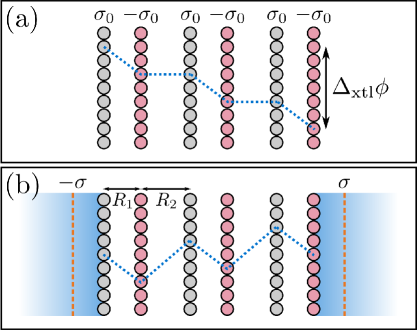
Figure 1: The unreconstructed Ag-(0001) and I-(000-1) surfaces require polarity compensation for large crystal sizes. (a) In vacuum, alternating layers of Ag+ (silver circles) and I- ions (pink circles), respectively carrying surface charge densities $\sigma_{0}$ and $-\sigma_{0}$, establish a potential drop $\Delta_{\rm xtl}\phi$ across the slab. $\Delta_{\rm xtl}\phi$ increases linearly with the width of the slab, resulting in a divergence of the surface energy. (b) In an aqueous electrolyte solution, a Helmholtz layer (orange dashes) with surface charge density $\sigma$ is established, which reduces $|\Delta_{\rm xtl}\phi|$. If $\sigma=\sigma_{\rm CNC}$, then $\Delta_{\rm xtl}\phi=0$, as shown. Blue dotted lines show schematic electrostatic potential profiles $\phi(z)$. The separations between crystal planes are given by $R_{1}$ and $R_{2}$.

The issue of incomplete screening under periodic boundary conditions (PBC) that are often used in molecular simulations has been the subject of recent investigations by Zhang et al Zhang and Sprik (2016b); Sayer, Zhang, and Sprik (2017); Sayer, Sprik, and Zhang (2019). In these studies, which build upon the work of Stengel, Spaldin and Vanderbilt Stengel, Spaldin, and Vanderbilt (2009), a theoretical framework with which to model uniform electric and electric displacements fields under PBC has been established. We refer to these techniques as the finite field methods. Based on thermodynamic arguments, Zhang and Sprik showed that the Hamiltonians Zhang and Sprik (2016a),

$$\mathcal{H}_{D}(\mathbf{p}^{N},\mathbf{r}^{N})=\mathcal{H}_{\rm PBC}(\mathbf{p}^{N},\mathbf{r}^{N})+\frac{\Omega}{8\pi}\big{(}D_{z}-4\pi P_{z}(\mathbf{r}^{N})\big{)}^{2},$$ (1)

and,

$$\mathcal{H}_{E}(\mathbf{p}^{N},\mathbf{r}^{N})=\mathcal{H}_{\rm PBC}(\mathbf{p}^{N},\mathbf{r}^{N})-\Omega P(\mathbf{r}^{N})E_{z},$$ (2)

generate dynamics for a system held under constant electric displacement field $D_{z}$ and constant electric field $E_{z}$, respectively. Both of these fields are aligned along the surface normal, which we take to be the $z$ direction in a Cartesian coordinate system. The momenta and positions of the particles are denoted by $\mathbf{p}^{N}$ and $\mathbf{r}^{N}$, respectively, and $\mathcal{H}_{\rm PBC}$ describes the kinetic energy, and the potential energy arising from molecular interactions. It is important to note that the use of 3D Ewald summation with tin-foil boundary conditions is implicitly assumed in $\mathcal{H}_{\rm PBC}$. The $z$ component of the polarization at time $t$ is given by,

$$P_{z}(t)=\frac{1}{\Omega}\sum_{i}q_{i}z_{i}(t),$$ (3)

where $\Omega$ is the total volume of the orthorhombic simulation cell, $z_{i}$ is the $z$-component of the $i^{\rm th}$ particle’s position, which carries a charge $q_{i}$. The polarization is defined as the time integral of the current, and the sum runs over all species in the system (including free ions). This means that the only source of electric displacement comes from charges at the ‘boundaries at infinity’. It is also important to note that the $z_{i}$ that enter Eq. 3 do not necessarily correspond to the particle’s position in the primary simulation cell; when a particle traverses the cell boundary, its position is followed out of the cell. This is known as the itinerant polarization Caillol (1994). We also stress that all fields ($D_{z}$, $E_{z}$ and $P_{z}$) that appear in Eqs. 1 and 2 are uniform, and that the forces derived from $\mathcal{H}_{E}$ and $\mathcal{H}_{D}$ apply both to the solvent/electrolyte, and the AgI ions. The finite field methods have been used to calculate the dielectric constant of pure water using both classical Zhang and Sprik (2016a) and ab initio molecular dynamics Zhang, Hutter, and Sprik (2016), as well as the conductivities and dielectric constants of aqueous electrolyte solutions Cox and Sprik (2019). They have also been used to compute the capacitance of the Helmholtz layer at charged interfaces Zhang and Sprik (2016b); Sayer, Zhang, and Sprik (2017); Sayer, Sprik, and Zhang (2019); Zhang (2018), including the polar NaCl (111) surfaces.

Armed with the Hamiltonians given by Eqs. 1 and 2, the premise of using the finite field methods to overcome the necessarily small widths of crystal is simple: If one can impose a field ($E_{z}$ or $D_{z}$) such that $|\Delta_{\rm xtl}\phi|=0$, then one can force the aqueous environment to provide the appropriate compensating charge. This was the approach adopted in Refs. Zhang and Sprik, 2016b; Sayer, Zhang, and Sprik, 2017; Sayer, Sprik, and Zhang, 2019 to calculate the capacitance of the Helmholtz layer. In these studies, the crystal was held fixed. Here we push the argument further and test whether or not enforcing a compensating charge is sufficient to stabilize AgI’s polar surfaces on timescales relevant to ice formation. Before pursuing this, however, we first briefly discuss the finite field methods in comparison to the popular Yeh-Berkowitz (YB) correction.

The YB correction was developed as a relatively inexpensive procedure to remove interactions between periodic images along the $z$-direction in simulations employing a slab geometry Yeh and Berkowitz (1999). It works by adding a force $F_{z,i}^{(\rm YB)}=-4\pi q_{i}P_{z}$ to each particle $i$ in the simulation. It is straightforward to verify that this is the same force arising from the second term in Eq. 1 with $D_{z}=0$. The equivalence of the $D_{z}=0$ ensemble and the YB correction has been previously acknowledged in Ref. Zhang and Sprik, 2016b, where it was also shown that the vacuum spacing normally employed is not a requirement. In the remainder of this section, we will explain the procedures for establishing the CNC conditions in the constant $E_{z}$ and $D_{z}$ ensembles, and then go on to directly compare results from simulations performed at $D_{z}=0$, $D_{z}=D_{\rm CNC}$ and $E_{z}=E_{\rm CNC}$, where $D_{\rm CNC}$ and $E_{\rm CNC}$ are the fields that impose the appropriate compensating charge. We undertake this task as the YB correction was explicitly used by Fraux and Doye Fraux and Doye (2014) in their study of ice formation at AgI. Moreover, in the supporting information, we argue that the ‘mirrored slab’ geometry employed by Zielke et al Zielke, Bertram, and Patey (2014), and Glatz and Sarupria Glatz and Sarupria (2016) corresponds on average to the $D_{z}=0$ ensemble. We will show that use of the $D_{z}=0$ ensemble has severe consequences regarding the stability of the crystal. Importantly, in cases where the slab is held fixed, we find that using $D_{z}=0$ rather than $D_{\rm CNC}$ or $E_{\rm CNC}$ has important implications for the structure of the water at the interface.

II.1 Establishing the CNC conditions

Here we briefly overview how $E_{\rm CNC}$ and $D_{\rm CNC}$ are determined. As the underlying theory has been given in detail elsewhere Sayer, Zhang, and Sprik (2017); Sayer, Sprik, and Zhang (2019), we limit ourselves to highlighting only the most salient aspects relevant to the current study. A more detailed derivation is given in the supporting information. We will work exclusively with the so-called ‘insulator centered supercell’ geometry (ICS), (see Fig. S3). In this setup, the length of the simulation cell is $L_{z}$, and the primary simulation cell spans $-L_{z}/2\leq z<L_{z}/2$. The AgI slab comprises $n+1$ layers of ions, where $n$ is an odd integer, and is centered around $z=0$. We initially consider a case where the regions above and below the crystal are filled with an aqueous electrolyte solution.

We begin by considering $E_{\rm CNC}$. The dark blue line in Fig. 2  shows $\phi(z)$ for a AgI slab with $n=17$, obtained from a simulation in which $E_{z}=0$. In this simulation, the crystal was immobile. The location of the Ag-(0001) and I-(000-1) are indicated by dashed lines at $z_{+}\approx-1.55$ nm and $z_{-}\approx 1.55$ nm, respectively. It is clear there is a potential drop across the slab of $\Delta_{\rm xtl}\phi\approx-3.33$ V, corresponding to an average electric field across the slab of approximately 1.1 V/nm. $E_{\rm CNC}$ can be found empirically by repeating the simulation, but imposing different values of $E_{z}$, and measuring $\Delta_{\rm xtl}\phi$ in each instance (see Fig. S4). For this system, we find $E_{\rm CNC}\approx-0.31$ V/nm. The resulting $\phi(z)$ is shown by the cyan line in Fig. 2. Whereas we have effectively eliminated $\Delta_{\rm xtl}\phi$, there is now a potential drop across the simulation cell $\Delta_{\rm cell}\phi\approx 3.64$ V. Despite the form of $\phi(z)$, it is important to realize that the particles do not experience an impulsive force as they traverse the cell boundary; the field exerts a force $q_{i}E_{z}$ on each particle, irrespective of the particle’s position. This can be seen from Eq. 2. Note that from the Maxwell relation $D_{z}=E_{z}+4\pi P_{z}$, we can obtain an estimate for $D_{\rm CNC}$ by measuring $\langle P\rangle_{E_{\rm CNC}}$, the average polarization at $E_{\rm CNC}$. In this instance, we find $\langle D\rangle_{E_{\rm CNC}}\approx-14.95$ V/nm. This can be used as a consistency check for theoretical predictions of $D_{\rm CNC}$. Following the symmetry-preserving mean-field theory of Hu Hu (2014), Pan et al.Pan, Yi, and Hu (2018) have recently derived an analytic formula for $E_{\rm CNC}$ for the case of two oppositely charged sheets (effectively $n=1$ in the current context), provided one has a reasonable estimate of the separation of the Helmholtz layer from the crystal. Generalizing such an approach for $n>1$ may prove fruitful for future studies.

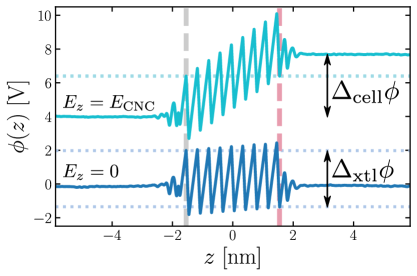
Figure 2: Establishing CNC conditions under constant $E_{z}$. The solid lines show $\phi(z)$ obtained at $E_{z}=0$ (dark blue) and $E_{\rm CNC}=-0.31$ V/nm (cyan). For clarity, the latter has been shifted up by 6 V. With $E_{z}=0$, there is a potential drop $\Delta_{\rm xtl}\phi\approx-3.33$ V across the slab, whereas at $E_{\rm CNC}$, there is instead a potential drop across the simulation cell, $\Delta_{\rm cell}\phi\approx 3.64$ V. The vertical dashed lines at $\pm 1.55$ nm indicate the surfaces of the crystal. The solution is an aqueous electrolyte, and results have been obtained at 298 K.

We now turn our attention to $D_{\rm CNC}$. While one could take the approach based on trial-and-error outlined above for $E_{\rm CNC}$, the $D_{z}$ ensemble lends itself to a more elegant solution. By solving a continuum Stern model, it was shown in Ref. Sayer, Sprik, and Zhang, 2019 that for the ICS, the CNC condition is simply,

$$D_{\rm CNC}=-4\pi\sigma_{\rm CNC},$$ (4)

where $\sigma_{\rm CNC}$ is the surface charge density of the Helmholtz layer such that polarity compensation is achieved. By solving a similar continuum Stern model, we show in the supporting information that,

$$\sigma_{\rm CNC}=\frac{(n+1)R_{1}}{(n+1)R_{1}+(n-1)R_{2}}\sigma_{0},$$ (5)

with $\sigma_{0}$ the surface charge density on each plane of the crystal, and $R_{1}$ and $R_{2}$ are the distances separating the planes (see Fig 1). For the wurtzite structure, $R_{2}/R_{1}=3.2$ such that $\lim_{n\to\infty}\sigma_{\rm CNC}\approx\sigma_{0}/4$, in agreement with Nosker et al. Nosker, Mark, and Levine (1970) For the AgI crystal with $n=17$ used in our simulations, Eqs. 4 and 5 give $D_{\rm CNC}=-14.99$ V/nm in good agreement with $\langle D\rangle_{E_{\rm CNC}}\approx-14.95$ V/nm obtained above. Performing a simulation at $D_{\rm CNC}$, we find $\Delta_{\rm xtl}\phi\approx 0.2$ V. In the case of a mobile slab, however, we have found it more robust to find $D_{\rm CNC}$ empirically from a simulation at $E_{\rm CNC}$. Table S1 gives the values of all fields used in our simulations.

The $E_{\rm CNC}$ and $D_{\rm CNC}$ conditions given above were derived in the case that the crystal was surrounded by an electrolyte solution. Given water’s ability to screen electric fields almost entirely, as characterized by its high dielectric constant, it is natural to ask whether or not pure water is able to provide polarity compensation. The trial-and-error approach for determining $E_{\rm CNC}$ described above provides a means for answering this question directly. If it is indeed found that water can provide polarity compensation, will the CNC conditions for the $D_{z}$ ensemble remain the same? We argue that the answer is ‘yes’. In the derivation of the CNC conditions for the electrolyte (see Refs.  Zhang and Sprik, 2016b; Sayer, Zhang, and Sprik, 2017; Sayer, Sprik, and Zhang, 2019 and supporting information), $D_{z}$ determines the value of the surface charge densities at the cell boundaries, and consquently the surface charge density of the Helmholtz layer. This is a direct consequence of a uniform polarization in the electrolyte. In the case of zero ionic strength, there is no longer a Helmholtz layer. Rather, a single boundary between the solvent and the crystal must provide the required charge compensation. If we were to observe a uniform solvent polarization, it stands to reason that as we require the same value of $\sigma_{\rm CNC}$, then the value of $D_{\rm CNC}$ will be the same at zero ionic strength as it is for the electrolyte.

II.2 Comparing $D_{z}=0$ with $E_{\rm CNC}$ and $D_{\rm CNC}$

As simulations of heterogeneous ice formation typically consider pure water in contact with an INP, the prospect of being able to enforce CNC without ions present is particularly intriguing, as it will permit a direct comparison of how different electrostatic boundary conditions affect the crystallization process. To this end, we have found $E_{\rm CNC}$ by trail-and-error for an immobile AgI crystal in contact with pure water. In Fig. 3, we show $\phi(z)$ at $D_{z}=0$ and $E_{z}=E_{\rm CNC}$. The result for $D_{z}=0$ is striking, with $|\Delta_{\rm xtl}\phi|\approx 46.2$ V corresponding to an average electric field of 14.9 V/nm across the slab. On the other hand, no such large electric field across the crystal is seen at $E_{\rm CNC}$ (albeit by construction). Rather, what is now observed is a uniform field in the solvent, $|E_{z,\rm solv}|\approx 0.39$ V/nm. Following our discussion at the end of Sec. II.1, we therefore expect the value of $D_{\rm CNC}$ to still be given by Eqs. 4 and 5. Indeed, we find $\langle D\rangle_{E_{\rm CNC}}\approx-14.92$ V/nm compared to the theoretical prediction of $D_{\rm CNC}=-14.99$ V/nm. Performing a simulation at the theoretical value of $D_{\rm CNC}$ gives $\phi(z)$ shown by the dotted line in Fig. 3, which agrees well with the profile obtained at $E_{\rm CNC}$.

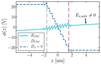
Figure 3: Comparing $\phi(z)$ from different ensembles for AgI ($n=17$) in contact with pure water at 298 K. At $D_{z}=0$ (dashed line) there is a large potential drop across the slab, $\Delta_{\rm xtl}\phi\approx-46.2$ V. At $E_{\rm CNC}$ (solid line), the potential drop is essentially zero by construction, but there is now a finite field in the solvent, $|E_{z,\rm solv}|\approx 0.39$ V/nm. The result obtained at $D_{\rm CNC}=-14.99$ V/nm (dotted line) agrees well with the $E_{\rm CNC}$ result. Note that the value of $D_{\rm CNC}$ is the same as that at finite ionic strength.

The consequences of such a large field across the crystal with $D_{z}=0$ are severe. This is demonstrated in Fig. 4 (a), which shows a snapshot from a $D_{z}=0$ simulation in which the Ag+ and I- ions are free to move. After just 50 ps, the slab no longer resembles the wurtzite structure of AgI. In contrast, at $E_{\rm CNC}$ or $D_{\rm CNC}$, the crystal remains close to the wurtzite structure, even on the nanosecond timescale, as shown in Fig. 4 (b) for $E_{\rm CNC}$. While the above results demonstrate the extreme care required when dealing with polar surfaces like those at AgI, it is still common practice to model crystalline lattices in contact with water as rigid substrates. One may therefore argue that enforcing CNC conditions by imposing $E_{\rm CNC}$ or $D_{\rm CNC}$ is only of secondary importance. However, even when using an immobile AgI crystal, the effects on the structure of the water in the contact layer are profound. This is demonstrated in Figs. 5 (a) and (b), where we show snapshots that focus on the contact layer from simulations at $D_{z}=0$ and $D_{\rm CNC}$, respectively. In the case of the former, we see a large proportion of water molecules directing O–H bonds toward the positively charged Ag-(0001) surface. In contrast, at $D_{\rm CNC}$ no O–H bonds are directed toward the interface. These observations from single snapshots are corroborated by Figs. 5 (c) and (d), where we show the probability distribution functions of the O–H bond orientations in the contact layer obtained from averages over the entire trajectory (see Sec. V.3). Also shown are distributions in the bulk region in both cases. At $D_{z}=0$, a uniform distribution of O–H bond orientations is observed. In contrast, at $D_{\rm CNC}$ there is a preference for O–H bonds to be directed away from the Ag-(0001) surface. This broken symmetry is consistent with $E_{z,\rm solv}\neq 0$ reported in Fig. 3. Below we will investigate the implications that these differences in interfacial liquid structure have for ice formation. However, we expect the behavior observed at the AgI/H2O interface to be similar at other polar substrates. Given the widespread use of the YB correction (or $D_{z}=0$ ensemble), we expect our findings to be important for the modeling of a wide variety of other systems too.

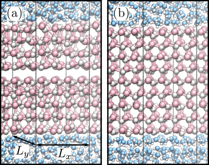
Figure 4: Snapshots from simulations with a mobile AgI crystal. (a) At $D_{z}=0$ the AgI loses its wurtzite crystal structure almost immediately (snapshot taken after 50 ps). (b) At $E_{\rm CNC}$, on the other hand, the AgI crystal maintains its crystal structure on the nanosecond timescale (snapshot taken after 1.6 ns). In both cases, the central plane of Ag+ and I- ions are held fixed. Color scheme: Ag+, silver; I-, pink; O, blue; and H, white. The black lines indicate the simulation cell boundaries. Only part of the simulation cell is shown. The solution is pure water, and results have been obtained at 298 K.

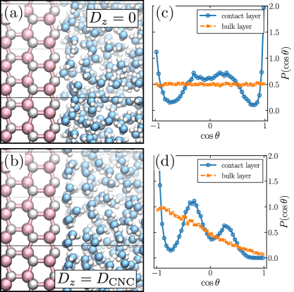
Figure 5: Electrostatic boundary conditions greatly influence the structure of water at the interface. (a) and (b) show close up snapshots of the Ag-(0001)/H2O interface with an immobile AgI crystal at 298 K, with $D_{z}=0$ and at $D_{\rm CNC}$, respectively. At $D_{z}=0$, a significant proportion of molecules in the contact layer direct O–H bonds toward the positively charged Ag-(0001) surface. In contrast, at $D_{\rm CNC}$ no O–H bonds are directed toward the interface, as seen in (b). Color scheme as in Fig. 4. Only part of the simulation cell is shown. (c) and (d) show $P(\cos\theta)$ at $D_{z}=0$ and $D_{\rm CNC}$, respectively, both for water molecules in the contact layer (blue circles) and in bulk solvent (orange squares), where differences in structure are also observed. $\cos\theta=+1$ and $\cos\theta=-1$ indicate O–H bonds directed immediately toward and away from Ag-(0001), respectively.

III Ice formation at silver iodide

III.1 Pure water

By enforcing CNC conditions with the finite field Hamiltonians (Eqs. 1 and 2), we have established that the polar Ag-(0001) and I-(000-1) surfaces are stable in an aqueous environment, at least on the nanosecond timescale. We have also observed pronounced differences in the structure of the interfacial water when simulated at $D_{z}=0$ and under CNC conditions. In the absence of ions, however, we also observed a finite field in the solvent, $|E_{z,\rm solv}|\approx 0.39$ V/nm. While a finite electric field inside a dielectric is not a problem in principle, in practice such a large field would likely lead to the dielectric breakdown of the water. Nevertheless, as simulations of ice formation at AgI have typically focused on systems at zero ionic strength Zielke, Bertram, and Patey (2014); Fraux and Doye (2014); Glatz and Sarupria (2016), it is instructive to compare and contrast ice formation for pure water in contact with AgI both at $D_{z}=0$ and at CNC conditions. Moreover, the pure water system acts as a useful (albeit unphysical) baseline to help understand the effects of ionic solutes.

To investigate ice formation, we adopted the simulation protocol outlined in Sec V. For each ensemble (i.e. $D_{z}=0$, $D_{z}=D_{\rm CNC}$ or $E_{z}=E_{\rm CNC}$), three simulations using this protocol were performed with an immobile AgI crystal. Under CNC conditions, simulations with a mobile AgI crystal were also performed; as this did not appear to greatly affect the mechanism, however, these results are included in the supporting information. In Fig. 6 (a) we show a representative snapshot of the system after ice formation with $D_{z}=0$. Consistent with previous studies, ice is seen to form preferentially at Ag-(0001) rather than I-(000-1). This demonstrates that our simulation setup is sufficiently robust to capture the general results of previous studies, despite the use of smaller simulation cells, and a lack of a vacuum gap between periodic replicas normal to the AgI surface. Under CNC conditions, this preference for ice formation at Ag-(0001) rather than I-(000-1) persists. However, the occurrence of significant transient ice-like structures is more pronounced at I-(000-1) under CNC conditions than it is at $D_{z}=0$, and indeed, in some of our simulations ice formation is observed at I-(000-1) as well as Ag-(0001), see Fig. S11.

How does the structure of the ice that forms at $D_{z}=0$ and under CNC conditions compare? In Figs. 6 (a) and (b) we show snapshots of the system after ice formation for each ensemble, along with the corresponding distributions of O–H bond orientations in Figs. 6 (c) and (d). It is apparent that the differences in liquid state structure reported in Fig. 5 greatly influence the structure of the ice that form. At $D_{z}=0$ we see O–H bonds directed toward and away from the interface, both in the contact layer, and in the ice that forms away from the surface. In contrast, at $D_{\rm CNC}$ no O–H bonds are directed toward Ag-(0001).

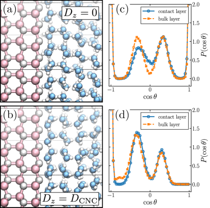
Figure 6: Differences in liquid structure persist upon ice formation. Panels (a)-(d) are analogous to those in Fig. 5, but here they are obtained after ice formation at 242 K (results shown for an immobile AgI crystal). At $D_{z}=0$, O–H bonds are directed both toward and away from the interface [(a) and (c)]. In contrast, at $D_{\rm CNC}$ no O–H bonds are directed toward Ag-(0001) [(b) and (d)].

III.2 Finite ionic strength

The ‘pure H2O + AgI’ system investigated in Sec. III.1 provides an interesting comparison study of the $D_{z}=0$ and CNC ensembles. Nevertheless, in both instances there are unphysical aspects. At $D_{z}=0$ it is not possible to simulate the crystal with mobile Ag+ and I- ions owing to a large potential drop across the slab. Conversely, under CNC conditions there is an unrealistically large electric field in the solvent. This is strong motivation to investigate the effects of ions on ice formation, as such mobile charge carriers may provide polarity compensation while maintaining zero electric field far from the crystal (see Fig. 2). Here we will restrict ourselves to a simple NaCl aqueous electrolyte for which reasonable simple point charge models are readily available Benavides et al. (2017). However, we emphasize that using the finite field methods to enforce CNC conditions can be readily applied to other systems too. As it is known experimentally that ions affect ice formation in nontrivial ways—both at AgI Reischel and Vali (1975) and other surfacesWhale et al. (2018); Kumar et al. (2018)—the work presented in this section serves as a platform from which to study ice formation in more complex electrolytes.

For the $E_{\rm CNC}$ and $D_{\rm CNC}$ ensembles, we simulated ice formation using the same protocol as for the pure water system (see Sec. V). In order to mitigate colligative effects, we decided to simulate three ion pairs, which is in principle sufficient to enforce CNC conditions (Eq. 5). In Fig. 7 (a) we show a snapshot after ice formation has occurred at $D_{\rm CNC}$ in the presence of a mobile AgI slab. As in the case without ions, ice formation is still observed to occur preferentially at Ag-(0001) rather than I-(000-1). However, while the structure of the water in the contact layer is similar to that seen in the absence of ions, it is now clear that this structure is lost further from the interface. This is shown quantitatively by the probability distribution functions of O–H bond orientations in Fig. 7 (b). By acting as hydrogen bond acceptors, it appears that the Cl- ions sufficiently disrupt the polar hydrogen bond network found under CNC conditions in the pure water case.

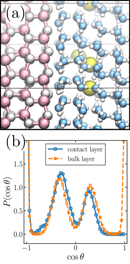
Figure 7: Ice formation in the presence of ions gives rise to a proton ordered contact layer, but proton disorder away from the surface. (a) Close up snapshot after ice formation at Ag-(0001) at 242 K, with a mobile AgI slab at $D_{\rm CNC}$. (b) $P(\cos\theta)$ both for the contact layer and a layer in the bulk. The Cl- ions are shown in yellow, otherwise the color scheme is the same as Fig. 4.

Finally, it is natural to ask about the effects of ions on the kinetics of ice formation. Given the small simulation cells and the limited number of simulations performed (three for each set of conditions), we are not in a position to make firm statements in this regard. Nevertheless, it does appear that ice formation is generally slower in the presence of dissolved ions, and undergoes a mechanism more akin to traditional nucleation i.e. a long induction time followed by relatively rapid crystal growth (see Figs. S9 and S10). These differences are particularly pronounced when compared to the $D_{z}=0$ ensemble results, where crystal formation appears especially fast. We also performed a set of simulations at $E_{\rm CNC}$ with a mobile AgI slab but with the signs of the dissolved ions swapped i.e. a hypothetical “Na- + Cl+” system. In this case, no ice formation was observed on the time scale of our simulations (approx. 350 ns). This null result indicates that ion specific details are indeed important for ice formation, and that the role of the ions extends beyond simply providing mobile charge to stabilize the surface.

IV Concluding Remarks

The focus of this article has been whether or not the polar Ag-(0001) and I-(000-1) surfaces of AgI are stable in aqueous solution on timescales relevant to ice formation. To achieve this, we have exploited recent advances in simulation methodology Zhang and Sprik (2016a, b); Sprik (2018) that enable us to enforce conditions of compensating net charge, thus ensuring that the drop in electrostatic potential across the crystal vanishes. This is a necessary condition for a finite surface free energy. We have found that under CNC conditions, the polar surfaces of AgI are indeed sufficiently stable to facilitate ice formation. Importantly, however, we have also found that the presence of dissolved ions is crucial in this regard; without these mobile charge carriers there exists a finite electric field in the aqueous phase. For the systems studied here, the magnitude of this field is unrealistically large. More generally, a finite uniform electric field will engender stability issues as the thickness of the liquid layer increases, in a similar manner to thin film polar oxides Noguera (2000); Goniakowski, Finocchi, and Noguera (2008). For macroscopic samples sizes, we conclude that the presence of mobile charge carriers is paramount for stability.

As discussed in the introduction, we have only considered a polarity compensation mechanism by which the aqueous environment supplies the required compensating charge, and we have neglected the possibility of electronic and nonstoichiometric reconstruction. This was motivated in part by the long held view that the close structural similarity between AgI and ice is the cause of its excellent ice nucleating properties Pruppacher and Klett (1997). The results presented here indeed suggest that this is a plausible explanation, although complicated by the polar surfaces’ need for proximate dissolved ions. While we cannot preclude electronic and nonstoichiometric reconstruction, a thorough study of the latter would likely require the development of improved force fields, while the former would call for explicit calculation of the electronic structure. These lie beyond the scope of the current article. Ultimately, the relative importance of these different mechanisms will be determined by the relative free energies and kinetic barriers separating the appropriate states. Enforcing CNC conditions in the presence of the aqueous environment will at the very least provide an appropriate reference state.

For pure water in contact with Ag-(0001) and I-(000-1) we also compared to simulations performed at $D_{z}=0$, which has the same Hamiltonian as the commonly used Yeh-Berkowitz method Yeh and Berkowitz (1999). We found the contrast with the system under CNC conditions to be stark: At $D_{z}=0$ a significant proportion of O–H bonds were found to be directed toward the positively charged Ag-(0001) surface, whereas under CNC conditions no O–H bonds were found to point at the surface. This difference in contact layer structure was seen to persist upon introduction of dissolved ions. We expect this result to have implications beyond the AgI system considered here. It is worth emphasizing that to enforce CNC conditions we have used two different methods: Imposing a uniform electric field, or imposing a uniform electric displacement field. The equations of motion for these two ensembles are different, and correspond to distinctly different electrostatic boundary conditions Zhang and Sprik (2016a); Sprik (2018). It is therefore rather satisfying that results obtained at $D_{\rm CNC}$ and $E_{\rm CNC}$ are broadly in agreement with each other.

Let us put this work in the context of ice nucleation more broadly. Throughout this study we have used relatively small simulation cells and “off-the-shelf” non-polarizable force fields. These have been sufficient for the purpose of demonstrating the effects of different electrostatic boundary conditions on the stability of Ag-(0001) and I-(000-1) in aqueous environments, and the potential impact this has for ice formation. To obtain quantitative kinetic data would require the use of much larger simulations in combination with e.g. seeding techniques Sanz et al. (2013); Espinosa et al. (2014); Pedevilla et al. (2018) or forward flux sampling Haji-Akbari and Debenedetti (2015); Bi, Cabriolu, and Li (2016); Cabriolu and Li (2015); Bi, Cao, and Li (2017); Sosso et al. (2016b, 2018) to compute rates, which should be readily compatible with the Hamiltonians given by Eqs. 1 and 2. The finite field methods used here can therefore be viewed as an additional tool for those investigating heterogeneous ice nucleation with computer simulation. Given it is becoming increasingly apparent that ions impact heterogeneous ice nucleation in complex ways Whale et al. (2018); Kumar et al. (2018), these techniques are likely to be important for many future studies in this area. Perhaps most importantly, what our results highlight is the crucial role ions can play in the heterogeneous ice formation mechanism itself, and should not be considered as a small perturbation to the water/solid interface.

V Methods

V.1 Force fields and molecular models

To model AgI we used a reparametrized version Shimojo and Kobayashi (1991); Bitrián and Trullàs (2008) of the Parrinello-Rahman-Vashista (PRV) force field Parrinello, Rahman, and Vashishta (1983). Non-electrostatic interactions were computed from a table, which gives consistent results with Ref. Bitrián and Trullàs, 2008 for molten AgI (see Fig. S18). To model water we used the TIP4P/2005 model Abascal and Vega (2005), which has a melting temperature $T_{\rm m}=252$ K. For sodium chloride we used the recently developed Madrid model Benavides et al. (2017), whose non-electrostatic interactions with water are of a simple Lennard-Jones (LJ) form. This model was designed specifically for use with TIP4P/2005, and gives a good description of the solubility of NaCl in water. With appropriate signs, silver and iodide ions carried a charge $q_{\ce{AgI}}=0.5815\,e$, while sodium and chloride ions carried a charge $q_{\ce{NaCl}}=0.85\,e$. Despite the use of these partial charges, for ease of notation we still refer to these ions as ‘Ag+’ etc. throughout the article. Oxygen atoms of the water molecule carried a charge $q_{\rm O}=-1.1128\,e$ and the charge on the hydrogen atoms was $q_{\rm H}=-q_{\rm O}/2$. Following Fraux and Doye Fraux and Doye (2014), who also used the TIP4P/2005 model in their study of ice formation at AgI, the non-electrostatic interactions between the AgI ions and the water molecules were described by a LJ potential centered on the oxygen atoms of the water molecules, using parameters originally from Hale and Keifer Hale and Kiefer (1980). Lorentz-Berthelot mixing rules were applied to obtain non-electrostatic interactions between NaCl and AgI. Parameters for non-electrostatic interactions are reported in Tables S2 and S3.

Following Zielke et al Zielke, Bertram, and Patey (2014), we used Burley’s lattice parameters ($a=0.4592$ nm, $c=0.7510$ nm) for AgI Burley (1963). All simulations used in this work comprised $n+1=18$ layers of AgI, with each layer itself comprising 16 Ag+ or I- ions. With the crystal held fixed, this resulted in a slab width of 3.0934 nm. The lateral dimensions of the simulation cell were $L_{x}=1.8368$ nm and $L_{y}=1.5907$ nm, resulting in a formal charge density on each layer of $\sigma_{0}\approx 3.18\,e/\text{nm}^{2}$. The total length of the simulation cell in the $z$-direction (which we take to be normal to the surface) was $L_{z}=11.7475$ nm. The remaining volume not occupied by AgI contained 750 water molecules, resulting in a number density in the bulk fluid region of $\rho_{\rm w}\approx 30.4\,\text{nm}^{-3}$ at 298 K. This is slightly lower than the density of bulk liquid water, and has been chosen as the finite field methods have been formulated strictly in the canonical ensemble Zhang and Sprik (2016a); Sprik (2018); using this lower density therefore allows enough space for the growing ice crystal. This is similar to the approach adopted by Zielke et al Zielke, Bertram, and Patey (2014). We note that, in contrast, Fraux and Doye used liquid films with one side in contact with AgI and the other in contact with vacuum, effectively holding the fluid at zero pressure. As our results without dissolved ions at $D_{z}=0$ appear broadly consistent with Fraux and Doye, it suggests the general features of ice formation at AgI are fairly robust to such simulation details. For simulations with dissolved ions, three NaCl ion pairs were placed in the fluid region, with no further adjustments to the simulation set up.

V.2 Simulation protocols

We have performed two types of simulations for the system described above. First, we have performed simulations at 298 K (i.e. water in the liquid state) in order to establish the CNC conditions (see Sec. II.1). Then, we have performed simulations with a protocol described below to observe ice formation. Throughout this article we used the LAMMPS simulation package Plimpton (1995), suitably modified to propagate dynamics in the constant $E_{z}$ and $D_{z}$ ensembles with the TIP4P/2005 water model. The velocity Verlet algorithm was used to propagate dynamics with a time step of 2 fs. To maintain the rigid geometry of the TIP4P/2005 water molecules, we used the RATTLE algorithm Andersen (1983). Temperature was maintained using a Nose-Hoover thermostat Shinoda, Shiga, and Mikami (2004); Tuckerman et al. (2006) with damping constant 0.2 ps. The particle-particle particle-mesh Ewald method was used to account for long-ranged interactions Hockney and Eastwood (1988), with parameters chosen such that the root mean square error in the forces were a factor $10^{5}$ smaller than the force between two unit charges separated by a distance of 1.0 ÅKolafa and Perram (1992).

For simulations performed at 298 K, at least 100 ps of equilibration was performed, followed by a further 1.5 ns of production. To compute the electrostatic potential profiles $\phi(z)$, the procedure outlined in Ref. Wirnsberger et al., 2016 was followed. To investigate ice formation, we used the following protocol. First, dynamics were propagated at 252 K for 5 ns. Then the system was cooled at a rate of 0.5 K/ns for 20 ns to a target temperature of 242 K. Finally, the dynamics of the system were propagated at 252 K until ice formation was observed, or 470 ns had occurred (whichever was sooner). Aside from the simulations in which we reversed the signs of the dissolved ions’ charge (see Sec. III.2), ice formation was observed in all but one simulation.

V.3 Bond orientation statistics

To quantify the bond orientation statistics at the interface, we have calculated $\cos\theta$, where $\theta$ is the angle formed between the O–H bond and the $z$-axis of the simulation cell. Specifically, if we denote the unit vector pointing from the oxygen atom of a water molecule to one of its hydrogen atoms (the procedure is repeated for the other hydrogen) as $\hat{\mathbf{b}}$ and the unit vector along the $z$-direction as $\hat{\mathbf{z}}$, then what we in fact calculate is $\hat{\mathbf{b}}\cdot\hat{\mathbf{z}}=\cos\theta$. In our simulation setup, the surface normal of Ag-(0001) points along $-\hat{\mathbf{z}}$, thus $\cos\theta=-1$ corresponds to an O–H bond directed away from the surface, and $\cos\theta=+1$ means an O–H bond is directed toward the surface. At I-(000-1) the situation is reversed, that is, $\cos\theta=-1$ corresponds to an O–H bond directed toward the surface, and $\cos\theta=+1$ means an O–H bond is directed away from the surface (see Fig. S12).