Superheating fields of semi-infinite superconductors and layered superconductors in the diffusive limit: structural optimization based on the microscopic theory

Abstract

We investigate the superheating fields $H_{sh}$ of semi-infinite superconductors and layered superconductors in the diffusive limit by using the well-established quasiclassical Green’s function formalism of the BCS theory. The coupled Maxwell-Usadel equations are self-consistently solved to obtain the spatial distributions of the magnetic field, screening current density, penetration depth, and pair potential. We find the superheating field of a semi-infinite superconductor in the diffusive limit is given by $H_{sh}=0.795H_{c0}$ at the temperature $T\to 0$. Here $H_{c0}$ is the thermodynamic critical-field at the zero temperature. Also, we evaluate $H_{sh}$ of layered superconductors in the diffusive limit as functions of the layer thicknesses ($d$) and identify the optimum thickness that maximizes $H_{sh}$ for various materials combinations. Qualitative interpretation of $H_{sh}(d)$ based on the London approximation is also discussed. The results of this work can be used to improve the performance of superconducting rf resonant cavities for particle accelerators.

I Introduction

The superconducting radio-frequency (SRF) resonant-cavity [1, 2] is the crucial component of modern particle accelerators, which efficiently imparts the electromagnetic energy to charged particles via the rf electric field. The accelerating gradient $E_{acc}$, namely, the average electric field that charged particles see during transit, is proportional to the amplitude $H_{0}$ of the rf magnetic field at the inner surface of the cavity, e.g., $\mu_{0}H_{0}=gE_{acc}$ and $g=4.26\,{\rm mT/(MV/m)}$ for the TESLA-shape cavity. Today, the best Nb cavities can reach $\mu_{0}H_{0}\sim 200\,{\rm mT}$, which corresponds to $E_{acc}\simeq 40$-$50\,{\rm MV/m}$ [3, 4, 5, 6, 7].

The ultimate limit of $H_{0}$ is thought to be around $H_{c}$, irrespective of whether the cavity material is a type-I or a type-II superconductor. Here, $H_{c}$ is the thermodynamic critical field. This limitation comes from the fact that an SRF cavity is operated under the Meissner state, and the upper critical field $H_{c2}$ is irrelevant to SRF in contrast to some dc applications. Let us consider a semi-infinite superconductor in the Meissner state shown in Fig. 1 (a) and suppose the penetration depth is given by $\lambda$. The external magnetic field $H_{0}\sim H_{c}$ induces the screening current density $j_{s}\sim H_{c}/\lambda$ at the surface, which is close to the depairing current density $j_{d}$, the stability limit of the superfluid flow. Hence, $H_{0}$ cannot substantially exceed $H_{c}$ as long as a simple semi-infinite superconductor is used. The value of $H_{0}$ which makes the Meissner state absolutely unstable is the so-called superheating field $H_{sh}\,(\sim H_{c})$.

In the Ginzburg-Landau (GL) regime, $H_{sh}$ of a semi-infinite superconductor has been thoroughly investigated [8, 9, 10]. However, the GL results are valid at a temperature $T$ close to the critical temperature $T_{c}$, while SRF cavities are operated at $T\ll T_{c}$ (e.g., $T/T_{c}\sim 0.1$-$0.2$ for Nb and ${\rm Nb_{3}Sn}$ cavities). Microscopic calculations of $H_{sh}$, which are valid at an arbitrary temperature $0<T<T_{c}$, have been carried out for extreme type-II superconductors, including clean-limit superconductors [11, 12, 13], superconductors including homogeneous [14] and inhomogeneous impurities [15], and dirty-limit superconductors with Dynes subgap states [16].

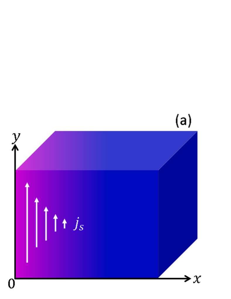
Figure 1: (a) Semi-infinite superconductor occupying $x\geq 0$. (b) Layered structure that consists of a thin superconducting layer (S) and a superconducting substrate (${\rm\Sigma}$). Here, we assume S is completely decoupled from ${\rm\Sigma}$: we do not consider neither the proximity effect nor any electron transfer between S and ${\rm\Sigma}$. The magnetic field $H_{0}$ is applied parallel to $z$ axis, and the screening current flows parallel to $y$ axis.

Besides the simple semi-infinite superconductor, the layered superconductor shown in Fig. 1 (b) has also attracted much attention from SRF researchers because of its potential for increasing the ultimate field-limit. Gurevich [17] proposed the idea of multilayer coating, which introduces a higher-$H_{c}$ superconducting (S) layer formed on the top of the superconducting substrate (${\rm\Sigma}$). Here, the S layer is decoupled from ${\rm\Sigma}$ by an insulator layer or a natural oxide layer. Using the London theory, it was later shown [18] that, when the penetration depth of the S layer is larger than that of the substrate ${\rm\Sigma}$, a current counterflow induced by ${\rm\Sigma}$ leads to a suppression of the current density in the S layer, resulting in an enhancement of the ultimate field-limit. The enhancement is maximized when the S layer has the optimum thickness $d=d_{m}\sim\lambda^{\rm(S)}$ [18]. It was also shown [19] that the similar consequences result from the GL calculations, which are valid at $T\simeq T_{c}$. However, we should use the microscopic theory for quantitative analyses. Fortunately, for a clean-limit $s$-wave superconductor at $T=0$, analyses based on the microscopic theory are significantly simplified. The nonlinear Meissner effect is negligible in this regime, and the London equation is valid even under a strong current density close to $j_{d}$. Combining the current distribution obtained from the London equation and $j_{d}$ for a clean-limit superconductor calculated from the microscopic theory, the more quantitative theory of the optimum multilayer is obtained [20]. These theoretical advances are discussed in detail in the review article [21]. Progress in experiments is summarized in Ref. [22] (see also progress in the last several years, e.g., Refs. [23, 24, 25, 28, 29, 26, 27, 30, 31, 32, 33, 34]).

Also, Nb cavities processed by some materials-treatment methods (e.g., $120^{\,\circ}{\rm C}$ baking, nitrogen infusion, etc.) are known to have a thin dirty-layer (S) on the surface of the bulk Nb (${\rm\Sigma}$) [35, 36, 6, 7], which can be modeled by the geometry shown in Fig. 1 (b). In fact, the calculations of the field-dependent nonlinear surface resistance [37, 38] have shown that layered structures can mitigate the quality factor degradation at high-fields. Moreover, it was shown [21, 15] that the thin dirty-layer at the surface improves $H_{sh}$ by the same mechanism as that in the S-${\rm\Sigma}$ heterostructure: a current counterflow induced by Nb substrate leads to a suppression of the current density in the dirty-Nb layer, resulting in an enhancement of $H_{sh}$. These theoretical results are qualitatively consistent with experiments [39, 40, 41, 6, 7]. Other effects resulting from the materials treatment (e.g., effects on hydride precipitate [42, 43]) may also play significant roles in the performance improvements, which can be incorporated considering imperfect surface-structures such as proximity-coupled normal layer on the surface [37, 38, 44, 45, 46, 47].

Despite the extensive studies, the superheating fields of a simple semi-infinite superconductor and a layered heterostructure in the diffusive limit have not yet been studied. Also, the structural optimization of a layered heterostructure in the diffusive limit has not yet been done. In this regime, we can no longer use the London equation at $j_{s}\sim j_{d}$ due to the nonlinear Meissner effect [48, 49, 15, 16] in contrast to the clean-limit regime. We need to self-consistently solve the microscopic theory of superconductivity combined with the Maxwell equations, incorporating the current-induced pair-breaking effect and the resultant nonlinear Meissner effect [14, 15, 16]. In the present work, we evaluate $H_{sh}$ for these geometries and identify the optimum thicknesses of layered structures.

The paper is organized as follows. In Section II, we briefly review the Eilenberger-Usadel-Larkin-Ovchinnikov formalism of the BCS theory in the diffusive limit and express physical quantities with the Matsubara Green’s functions. The solutions of the Usadel equation at $T=0$ and the analytical expression of the depairing current density are also summarized. In Sec. III, we consider a simple semi-infinite superconductor [see Fig. 1 (a)]. The coupled Maxwell-Usadel equations are self-consistently solved to obtain the spatial distributions of the magnetic field $H(x)$, the current density $j_{s}(x)$, pair potential $\Delta(x)$, and the penetration depth $\lambda(x)$. Then, the superheating field in the diffusive limit is derived. In Sec. IV, we consider a layered superconductor [see Fig. 1 (b)], self-consistently solve the coupled Maxwell-Usadel equations, and obtain the spatial distributions of $H(x)$, $j_{s}(x)$, $\Delta(x)$, and $\lambda(x)$. Then, we evaluate $H_{sh}$ as functions of the S-layer thickness $d$ for various material combinations and find the optimum thickness $d_{m}$. Qualitative interpretation of the results are also discussed using an approximate formula of $H_{sh}(d)$. In Sec. V, we discuss the implications of our results.

II Theory

II.1 Eilenberger-Usadel-Larkin-Ovchinnikov formalism

Let us briefly summarize the well-established Eilenberger-Usadel-Larkin-Ovchinnikov formalism of the BCS theory in the diffusive limit [47, 50, 51, 52, 53]. Here we assume the current distribution varies slowly over the coherence length. Then, the normal and anomalous quasiclassical Matsubara Green’s functions $G_{\omega_{n}}=\cos\theta$ and $F_{\omega_{n}}=\sin\theta$ and the pair potential $\Delta$ obey

$$\biggl{(}\Delta-\frac{s}{\sqrt{1+\cot^{2}\theta}}\biggr{)}\cot\theta=\hbar\omega_{n},$$ (1)

$$\ln\frac{T_{c}}{T}=2\pi k_{B}T\sum_{\omega_{n}>0}\biggl{(}\frac{1}{\hbar\omega_{n}}-\frac{\sin\theta}{\Delta}\biggr{)}.$$ (2)

Here $s=(q/q_{\xi})^{2}\Delta_{0}$ is the superfluid flow parameter, $\Delta_{0}=\Delta(s,T)|_{s=0,\,T=0}$ is the BCS pair potential for the zero-current state at $T=0$, $\hbar q$ is the superfluid momentum, $q_{\xi}=\sqrt{2\Delta_{0}/\hbar D}$ is the inverse of the coherence length, $D$ is the electron diffusivity, $\hbar\omega_{n}=2\pi k_{B}T(n+1/2)$ is the Matsubara frequency, $k_{B}T_{c}=\Delta_{0}\exp(\gamma_{E})/\pi\simeq\Delta_{0}/1.76$ is the BCS critical temperature, and $\gamma_{E}=0.577$ is the Euler constant. The penetration depth $\lambda$ and the magnitude of supercurrent density $j_{s}$ are given by

$$\frac{\lambda_{0}^{2}}{\lambda^{2}(s,T)}=\frac{4k_{B}T}{\Delta_{0}}\sum_{\omega_{n}>0}\sin^{2}\theta,$$ (3)

$$\frac{j_{s}(s,T)}{j_{s0}}=\sqrt{\frac{\pi s}{\Delta_{0}}}\frac{\lambda_{0}^{2}}{\lambda^{2}(s,T)}.$$ (4)

Here $\lambda_{0}=\lambda(0,0)=\sqrt{\hbar/\pi\mu_{0}\Delta_{0}\sigma_{n}}$ is the BCS penetration depth at $T=0$, $\sigma_{n}=2N_{0}De^{2}$ is the normal state conductivity, $N_{0}$ is the normal state density of states at the Fermi energy, $j_{s0}=H_{c0}/\lambda_{0}=\sqrt{\pi}|e|N_{0}D\Delta_{0}q_{\xi}$, and $H_{c0}=\sqrt{N_{0}/\mu_{0}}\Delta_{0}$ is the BCS thermodynamic critical field at $T=0$.

In the geometries shown in Figs. 1 (a) and 1 (b), the magnetic field and the superfluid flow depend on the depth $x$ from the surface. These $x$ dependences are determined from the Maxwell equations, $j_{s}=-\partial_{x}H$ and $\mu_{0}H=(\hbar/2|e|)\partial_{x}q$, namely,

$$\frac{\partial^{2}q}{\partial x^{2}}=\frac{q}{\lambda^{2}(s,T)},$$ (5)

$$\frac{H}{H_{c0}}=\sqrt{\pi}\frac{\partial(q/q_{\xi})}{\partial(x/\lambda_{0})}.$$ (6)

Suppose the magnetic field at the surface is given by $H_{0}$. Then, the boundary conditions can be written as

$$H(0)=H_{0},\hskip 51.21504pt\lim_{x\to\infty}q(x)\to 0.$$ (7)

For the geometry shown in Fig. 1 (b), we have the additional boundary conditions at the S-${\rm\Sigma}$ interface,

$$H(d_{-})=H(d_{+}),\hskip 28.45274ptq(d_{-})=q(d_{+}).$$ (8)

Here $d_{\pm}=d\pm 0$: we assume the thickness of the insulator or natural oxide layer separating S and ${\rm\Sigma}$ is negligible compared with $\lambda$ but thick enough to electrically decouple S and ${\rm\Sigma}$.

II.2 Solutions and depairing current at $T\to 0$

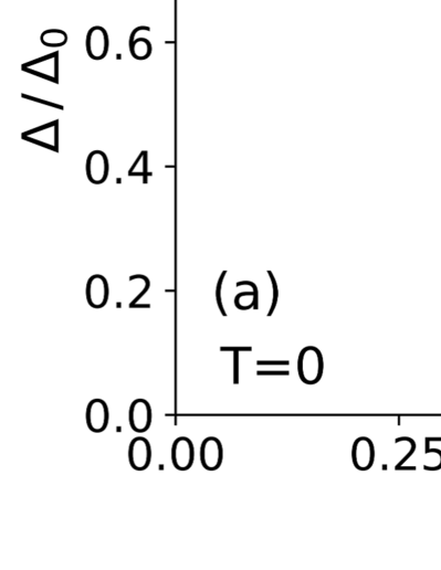
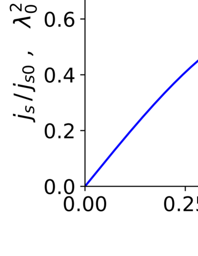
Figure 2: (a) Pair potential $\Delta$, (b) superfluid density $\lambda_{0}^{2}/\lambda^{2}$ and supercurrent density $j_{s}$ as a function of the superfluid momentum $|q/q_{\xi}|\,(=\sqrt{s/\Delta_{0}})$ calculated from the Usadel equation at $T\to 0$ [Eqs. (A) and (26), see Appendix A]. For $0\leq|q/q_{\xi}|\leq 0.675$, we can use Eqs. (9)-(11). The blob at $(0.487,0.595)$ indicates the depairing momentum and depairing current density.

For $T\to 0$, the Matsubara sum is replaced with an integral, and Eqs. (1)-(4) reduce to the well-known formulas obtained by Maki many years ago [54, 55, 56, 16] (see also Appendix A),

$$\frac{\Delta(s,0)}{\Delta_{0}}=\exp\biggl{[}-\frac{\pi s}{4\Delta(s,0)}\biggr{]},$$ (9)

$$\frac{\lambda_{0}^{2}}{\lambda^{2}(s,0)}=\frac{\Delta(s,0)}{\Delta_{0}}\biggl{[}1-\frac{4s}{3\pi\Delta(s,0)}\biggr{]},$$ (10)

$$j_{s}(s,0)=\sqrt{\frac{\pi s}{\Delta_{0}}}\frac{\Delta(s,0)}{\Delta_{0}}\biggl{[}1-\frac{4s}{3\pi\Delta(s,0)}\biggr{]}\frac{H_{c0}}{\lambda_{0}},$$ (11)

for $0\leq s\leq\Delta(s,0)$, namely, $0\leq s\leq 0.456\Delta_{0}$ or $0\leq|q/q_{\xi}|\leq 0.675$. Shown in Fig. 2 are $\Delta$, $\lambda$, and $j_{s}$ at $T=0$ as functions of $|q|$. While $\Delta$ and the superfluid density $\lambda_{0}^{2}/\lambda^{2}$ are monotonically decreasing functions, $j_{s}$ exhibits a non-monotonic behavior. At smaller $|q|$ regions, $j_{s}$ is proportional to $|q|$. As $|q|$ increases, $j_{s}$ becomes dominated by a rapid reduction of the superfluid density and ceases to increase. At a threshold value $q_{d}$, $j_{s}$ reaches the maximum value: the depairing current density $j_{d}$ [see the blob in Fig. 2 (b)].

Using Eqs. (9)-(11) and the condition $\partial_{s}j_{s}=0$, we have [54, 55, 57]

$$j_{d}(0)=\sqrt{\frac{\pi s_{d}}{\Delta_{0}}}\frac{\Delta_{d}}{\Delta_{0}}\biggl{(}1-\frac{4\zeta_{d}}{3\pi}\biggr{)}\frac{H_{c0}}{\lambda_{0}}=0.595\frac{H_{c0}}{\lambda_{0}},$$ (12)

$$\zeta_{d}=\frac{s_{d}}{\Delta_{d}}=\frac{2}{\pi}+\frac{3\pi}{8}-\sqrt{\biggl{(}\frac{2}{\pi}+\frac{3\pi}{8}\biggr{)}^{2}-1}=0.300,$$ (13)

$$\Delta_{d}=\Delta_{0}e^{-\frac{\pi}{4}\zeta_{d}}=0.790\Delta_{0},$$ (14)

$$s_{d}=\Delta_{d}\zeta_{d}=0.237\Delta_{0},$$ (15)

$$q_{d}/q_{\xi}=\sqrt{s_{d}/\Delta_{0}}=0.487,$$ (16)

which are the well-known formula of the depairing current density for a dirty BCS superconductor (see also Refs. [56, 16]).

In the following, we use $\Delta_{0}$ as a unit of energy and use dimensionless quantities $\tilde{s}=s/\Delta_{0}$, $\tilde{\omega}_{n}=\hbar\omega_{n}/\Delta_{0}$, $\tilde{\Delta}=\Delta/\Delta_{0}$, $\tilde{T}=k_{B}T/\Delta_{0}$, etc. For brevity, we omit all these tildes. Also, since we are interested in $H_{sh}$ at the operating temperature of SRF cavities ($T\ll T_{c}$), we consider $T\to 0$ for simplicity.

III Semi-infinite superconductor

III.1 Spatial distributions of $H$, $j_{s}$, $\Delta$, and $\lambda$

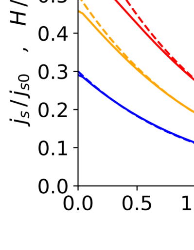
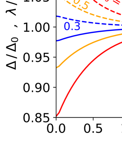
Figure 3: Spatial distributions of (a) $H$, $j_{s}$, (b) $\lambda$, and $\Delta$ obtained from the self-consistent solutions of the coupled Maxwell-Usadel equations [Eqs. (5)-(11)]. For $H_{0}\sim H_{c0}$ (red), the nonlinear Meissner effect manifests itself in the vicinity of the surface.

First, consider the semi-infinite superconductor shown in Fig. 1 (a) and self-consistently solve the coupled Maxwell-Usadel equations at $T\to 0$ [Eqs. (5)-(11)]. Shown in Fig. 3 (a) are the distributions of $H(x)$ and $j_{s}(x)$. For $H_{0}\ll H_{c0}$ (blue), we have the solid and dashed curves that almost overlap, which can be understood as follows. Since the current density is so small that the nonlinear Meissner effect is negligible, the London theory is applicable. Solving the London equation, we obtain $H(x)/H_{c0}=j_{s}(x)/j_{s0}=\exp(-x/\lambda_{0})$, consistent with the numerical solutions. As $H_{0}$ increases (orange and red), however, the nonlinear Meissner effect manifests itself, and the London theory is not applicable. In fact, the solid and dashed curves no longer overlap. Shown in Fig. 3 (b) are the penetration depth $\lambda(x)$ and the pair potential $\Delta(x)$. The pair potential (penetration depth) is decreased (increased) at the surface due to the strong pair-breaking current and recovers at deeper regions where the current density is exponentially small.

III.2 Superheating field

For a simple semi-infinite superconductor in the diffusive limit, in which the current density is a monotonically decreasing function of $x$ (see Fig. 3), the superheating field $H_{sh}$ is given by $H_{0}$ which induces $j_{s}(x)|_{x=0}=j_{d}$. Then, we can derive a simple formula of $H_{sh}$. Integrating both the sides of Eq. (5) from $x=0$ to $\infty$, we obtain $q^{\prime}(0)^{2}=-2\int_{0}^{\infty}qq^{\prime}\lambda^{-2}(s,T)dx$. Using Eqs. (6) and (7), we find the relation between $H_{0}$ and $s(x)|_{x=0}$: $(H_{0}/H_{c0})^{2}=\pi\int_{0}^{s(0)}ds[\lambda_{0}/\lambda(s,T)]^{2}$. Substituting the depairing value $s_{d}$ into $s(0)$, we obtain the formula [16]

$$H_{sh}(T)=H_{c0}\sqrt{\pi\int_{0}^{s_{d}}\!\!\!\!ds\frac{\lambda_{0}^{2}}{\lambda^{2}(s,T)}},$$ (17)

which is valid for an arbitrary $T$. Note that Eq. (17) reproduces the GL superheating field $H_{sh}(T)=(\sqrt{5}/3)H_{c}(T)$ at $T\simeq T_{c}$ [16], consistent with the previous studies [8, 9].

For $T=0$, substituting Eqs. (10) and (15) into Eq. (17), we obtain $H_{sh}$ in the diffusive limit [16]

$$H_{sh}(0) = H_{c0}\sqrt{1-\biggl{(}1-\frac{\pi\zeta_{d}}{2}\biggr{)}e^{-\frac{\pi\zeta_{d}}{2}}-\frac{2}{3}s_{d}^{2}}$$ (18)

$$= 0.795H_{c0}.$$

This is slightly smaller than that of an extreme type-II ($\lambda/\xi\gg 1$) superconductor in the clean limit [11, 12],

$$H_{sh}^{\rm clean}(0)=0.84H_{c0},$$ (19)

and consistent with the previous study on the effect of nonmagnetic impurities [14], in which $H_{sh}\,(\sim 0.8H_{c0})$ as a function of the mean free path $\ell$ takes its maximum value at $\ell=5.32\xi_{0}=\ell_{*}$ and decreases with $\ell$ for $\ell<\ell_{*}$.

IV Layered superconductors

Now we consider the layered heterostructure shown in Fig. 1 (b). The model parameters are summarized in Table. 1: the S-layer thickness $d$ and the three ratios of materials parameters,

$$r_{\Delta}=\frac{\Delta_{0}^{\rm(S)}}{\Delta_{0}^{\rm(\Sigma)}},\hskip 19.91684ptr_{H}=\frac{H_{c0}^{\rm(S)}}{H_{c0}^{\rm(\Sigma)}},\hskip 19.91684ptr_{\sigma}=\frac{\sigma_{n}^{\rm(S)}}{\sigma_{n}^{\rm(\Sigma)}}.$$ (20)

Here $\Delta_{0}^{(i)}$ ($i={\rm S},\,{\rm\Sigma}$) is the pair-potential in the zero-current state at $T=0$, $H_{c0}^{(i)}$ is the thermodynamic critical field at $T=0$, and $\sigma_{n}^{(i)}$ is the normal-state conductivity. The other materials parameters can be expressed using these parameters; e .g., $D^{\rm(S)}/D^{\rm(\Sigma)}=r_{\sigma}r_{\Delta}^{2}/r_{H}^{2}$, $\lambda_{0}^{({\rm S})}/\lambda_{0}^{({\rm\Sigma})}=1/\sqrt{r_{\Delta}r_{\sigma}}$, etc.

Table 1: Parameters of the layered structure.

S layer thickness	$d$,
Pair-potential ratio	$r_{\Delta}=\Delta_{0}^{\rm(S)}/\Delta_{0}^{\rm(\Sigma)}$,
Critical-field ratio	$r_{H}=H_{c0}^{\rm(S)}/H_{c0}^{\rm(\Sigma)}$,
Normal-conductivity ratio	$r_{\sigma}=\sigma_{n}^{\rm(S)}/\sigma_{n}^{\rm(\Sigma)}$.

IV.1 Spatial distributions of $H$, $j_{s}$, $\Delta$, and $\lambda$ in a layered superconductor

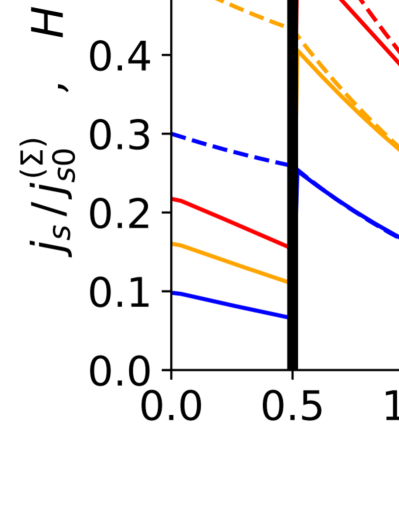
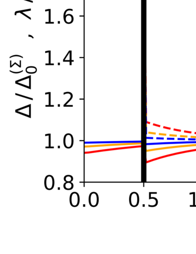
Figure 4: Spatial distributions of (a) $H$, $j_{s}$, (b) $\Delta$, and $\lambda$ in a layered superconductor calculated for $d=0.5\lambda_{0}^{\rm(\Sigma)}$, $r_{\Delta}=r_{H}=1$, and $r_{\sigma}=0.25$. The penetration depth of the S layer in the zero-current state is given by $\lambda_{0}^{\rm(S)}=\lambda_{0}^{\rm(\Sigma)}/\sqrt{r_{\Delta}r_{\sigma}}=2\lambda_{0}^{\rm(\Sigma)}$.

We can consider any materials combination, but here we focus on the simplest example that captures the striking feature of the layered structure: the surface-current-reduction effect. Let us assume that the S layer is made of the same material as the ${\rm\Sigma}$ region but has a different concentration of nonmagnetic impurities, e.g., ${\rm\Sigma}$ and S are a bulk Nb and a dirtier Nb-layer, respectively. We can fully solve the coupled Maxwell-Usadel equations at $T\to 0$ [Eqs. (5)-(11)] in the similar way as done for a semi-infinite superconductor in Sec. III.1. Shown in Fig. 4 are the distributions of $H(x)$, $j_{s}(x)$, $\lambda(x)$, and $\Delta(x)$ calculated for $d=0.5\lambda_{0}^{\rm(\Sigma)}$, $r_{\Delta}=r_{H}=1$, and $r_{\sigma}=0.25$. In the S layer, the magnetic field $H$ (dashed curves) slowly attenuates as $x$ increases, and the current density $j_{s}=-\partial_{x}H$ (solid curves) is significantly suppressed. As a result, $\Delta$ in the S region is less suppressed as compared with that in the ${\rm\Sigma}$ region, even though it is the S layer which is directly exposed to the external magnetic field [see the solid curves in Fig. 4 (b)]. In the ${\rm\Sigma}$ region, $H(x)$, $j_{s}(x)$, $\lambda(x)$, and $\Delta(x)$ monotonically decay as $x$ increases.

The non-monotonic decay of the current density is a common feature in the S-${\rm\Sigma}$ hetero-structure in which S has a different penetration depth from ${\rm\Sigma}$ [18, 19, 20, 21, 15]. When ${\rm\Sigma}$ has a shorter (longer) penetration depth than S, the magnetic field in the S layer decays slower (more rapid) than exponential, and the current density is suppressed (enhanced). Such reduction (enhancement) of the surface current results from a counterflow induced by the substrate ${\rm\Sigma}$. When the penetration depths in S and ${\rm\Sigma}$ are balanced, the magnetic field and the current density in the S layer exhibit the well-known exponential decay.

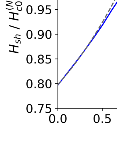
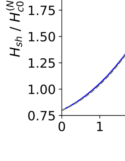
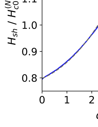
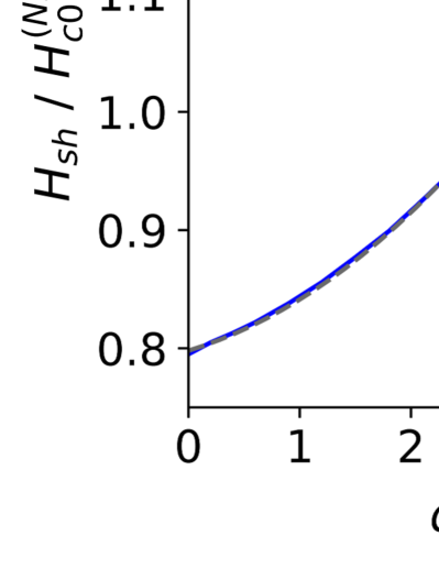
Figure 5: Superheating field of layered structures as functions of $d$. The solid curves are obtained from the self-consistent solutions of the coupled Maxwell-Usadel equations at $T\to 0$ [Eqs. (5)-(11)]. The dashed curves are calculated from the approximate formula [Eq. (21)]. (a) Nb-Nb structure modeled by the parameter set $(r_{\Delta},r_{H},r_{\sigma})=(1,1,0.25)$. (b) ${\rm Nb_{3}Sn}$-Nb structure modeled by $(r_{\Delta},r_{H},r_{\sigma})=(2,2.7,0.1)$. (c) NbN-Nb structure modeled by $(r_{\Delta},r_{H},r_{\sigma})=(1.7,1.15,0.03)$. (d) NbTiN-Nb structure modeled by $(r_{\Delta},r_{H},r_{\sigma})=(1.8,1.15,0.02)$. In these cases, the penetration depths of the S layer in the zero-current state are given by (a) $\lambda_{0}^{\rm(S)}=\lambda_{0}^{\rm(\Sigma)}/\sqrt{r_{\Delta}r_{\sigma}}=2\lambda_{0}^{\rm(\Sigma)}$, (b) $\lambda_{0}^{\rm(Nb_{3}Sn)}=2.2\lambda_{0}^{\rm(Nb)}$, (c) $\lambda_{0}^{\rm(NbN)}=4.4\lambda_{0}^{\rm(Nb)}$, and (d) $\lambda_{0}^{\rm(NbTiN)}=5.3\lambda_{0}^{\rm(Nb)}$.

IV.2 Superheating field of a layered superconductor

Next, we evaluate $H_{sh}$ of the layered structure. Since the current density in the layered structure does not necessarily take its maximum value at $x=0$ as seen in Fig. 4, the $H_{sh}$ formula given by Eq. (17) is not applicable. Instead, $H_{sh}$ is given by the surface magnetic-field which induces $j_{s}=j_{d}^{({\rm S})}$ at $x=0$ or $j_{s}=j_{d}^{({\rm\Sigma})}$ at $x=d$. Shown as the solid curves in Fig. 5 are $H_{sh}$ as functions of $d$ calculated from the coupled Maxwell-Usadel equations for various materials combinations. We find $H_{sh}$ increases with $d$, takes its maximum value at $d=d_{m}\sim\lambda_{0}^{({\rm S})}$, and decreases with $d$ at $d>d_{m}$.

Let us interpret these results by using an approximate formula. Neglecting the nonlinear Meissner effect and solving the London equation, we obtain the well-known formula [18, 19, 20, 21]:

$$H_{sh}(d)={\rm min}\Bigl{[}c_{1}(d)H_{sh}^{\rm(S)},c_{2}(d)H_{sh}^{\rm(\Sigma)}\Bigr{]},$$ (21)

$$c_{1}(d)=\frac{\cosh[d/\lambda_{0}^{\rm(S)}]+[\lambda_{0}^{\rm(\Sigma)}/\lambda_{0}^{\rm(S)}]\sinh[d/\lambda_{0}^{\rm(S)}]}{\sinh[d/\lambda_{0}^{\rm(S)}]+[\lambda_{0}^{\rm(\Sigma)}/\lambda_{0}^{\rm(S)}]\cosh[d/\lambda_{0}^{\rm(S)}]},$$ (22)

$$c_{2}(d)=\cosh[d/\lambda_{0}^{\rm(S)}]+[\lambda_{0}^{\rm(\Sigma)}/\lambda_{0}^{\rm(S)}]\sinh[d/\lambda_{0}^{\rm(S)}].$$ (23)

Here, $H_{sh}^{\rm(S)}$ and $H_{sh}^{\rm(\Sigma)}$ are the superheating field of a semi-infinite superconductor made from the S material and the ${\rm\Sigma}$ material, respectively. We use the values obtained from the microscopic theory in the diffusive limit: $H_{sh}^{\rm(\Sigma)}=0.795H_{c0}^{\rm(\Sigma)}$ and $H_{sh}^{\rm(S)}=0.795\,r_{H}H_{c0}^{\rm(\Sigma)}$ [see Eq. (18)]. The penetration depth of the S layer in the zero-current state is given by $\lambda_{0}^{\rm(S)}=\lambda_{0}^{\rm(\Sigma)}/\sqrt{r_{\Delta}r_{\sigma}}$. Shown as the dashed gray curves in Fig. 5 are $H_{sh}(d)$ calculated from Eq. (21). The existence of the optimum thickness $d_{m}$ can be understood as follows [18, 19, 20, 21]. Suppose $\lambda_{0}^{\rm(S)}>\lambda_{0}^{\rm(\Sigma)}$. Then, the counterflow induced by ${\rm\Sigma}$ decreases the current density at the surface of S by a factor of $1/c_{1}$, and the maximum field that the S layer can withstand increases to $H_{0}=c_{1}H_{sh}^{\rm(S)}$. This enhancement is pronounced as $d$ decreases. On the other hand, the S layer attenuate the magnetic field down to $H_{i}=H_{0}/c_{2}$ at the S-${\rm\Sigma}$ interface, so the maximum field that ${\rm\Sigma}$ can withstand is given by $H_{0}=c_{2}H_{sh}^{\rm(\Sigma)}$, which increases with $d$. The interplay between the reduction of the surface current and that of the shielding efficiency results in the existence of the optimum thickness $d_{m}$, at which the screening current densities in S and ${\rm\Sigma}$ simultaneously reach $j_{d}^{({\rm S})}$ and $j_{d}^{({\rm\Sigma})}$, respectively.

The disagreements between the full calculations (solid) and the approximate formula (dashed) result from the nonlinear Meissner effect. The strong current density $\sim j_{d}$ increases the penetration depth from $\lambda_{0}$ to $\lambda(s,0)|_{s\simeq s_{d}}$, so that a larger $d$ becomes necessary to protect ${\rm\Sigma}$ than expected from the London theory. As a result, the maximum in $H_{sh}(d)$ obtained from the full calculation is located at thicker regions.

Note $H_{sh}$ can decrease when S has a shorter penetration depth than ${\rm\Sigma}$. In this case, the current density in the S layer is enhanced as mentioned in Sec. IV.1 and can reach the depairing current density at rather small $H_{0}$. For instance, $(r_{\Delta},r_{H},r_{\sigma})=(1,1,4)$, which yields $\lambda_{0}^{\rm(S)}=\lambda_{0}^{\rm(\Sigma)}/\sqrt{r_{\Delta}r_{\sigma}}=0.5\lambda_{0}^{\rm(\Sigma)}<\lambda_{0}^{\rm(\Sigma)}$, results in $H_{sh}=0.46H_{c0}^{\rm(\Sigma)}$ for $d=0.05\lambda_{0}^{\rm(\Sigma)}$.

V Discussions

We have investigated a simple semi-infinite superconductor shown in Fig. 1 (a) and a layered heterostructure shown in Fig. 1 (b) in the diffusive limit. The coupled Maxwell-Usadel equations at $T\to 0$ have been self-consistently solved to obtain the spatial distributions of $H(x)$, $j_{s}(x)$, $\lambda(x)$, and $\Delta(x)$ for both the structures [see Figs. 3 and 4]. The distributions of $H$ and $j_{s}$ obey the London theory for $j_{s}\ll j_{d}$, while the nonlinear Meissner effect manifests itself for $j_{s}\sim j_{d}$, where the London theory is no longer valid. We have found the superheating field $H_{sh}$ of a semi-infinite superconductor in the diffusive limit is given by $H_{sh}=0.795H_{c0}$ at $T\to 0$; on the other hand, $H_{sh}$ of a layered structure depends on materials combinations and the thickness $d$ of the S layer, which can be maximized by tuning $d$ to the optimum thickness [see Fig. 5].

Our results can be tested by experiments. We can expect that the maximum operating field of an SRF cavity made from a bulk dirty-BCS-superconductor is given by its superheating field. Taking impurity-doped dirty Nb with $\ell\ll\xi$, for example, we have $\mu_{0}H_{sh}=0.795\times 200\,{\rm mT}=160\,{\rm mT}$ at $T\to 0$. The maximum operating field can be improved by applying a layered structure onto the inner surface of a cavity. For instance, $H_{sh}$ of bulk dirty Nb is pushed up to $\mu_{0}H_{sh}=1.04\times 200\,{\rm mT}=210\,{\rm mT}$ by laminating a thin dirtier-Nb-layer on the surface [see Fig. 5 (a)]. Other materials combinations can also improve the field limit, e.g., $\mu_{0}H_{sh}=2.26\times 200\,{\rm mT}=450\,{\rm mT}$ for the ${\rm Nb_{3}Sn}$-Nb structure [see Fig. 5 (b)]. These results can be tested using various techniques, e.g., high power rf pulse [58], rf characterization of samples [59, 60, 61, 30], third-harmonic voltage [62, 25, 34, 26, 27], magnetization measurements for ellipsoid samples [23], muon-spin-rotation technique [24, 63], etc. Note that the rf heating of the cavity wall due to quasiparticles [38, 44, 64, 65], vortices [66, 67, 68, 69, 70, 71, 72, 73, 74], topographic defects at the surface [75, 76, 77, 78, 79, 80, 81, 82, 83], and grain boundaries [84] can limit the achievable field.

The approximate formula [Eq. (21)], which was derived using the London equation [18], would be useful to know the optimum thickness $d_{m}$. For a clean-limit superconductor at $T=0$, the nonlinear Meissner effect is negligible. Hence, simply substituting the clean-limit result $H_{sh}^{(i)}=0.84H_{c0}^{(i)}$ into Eq. (21), we obtain the microscopically valid theory [20]. On the other hand, for a dirty-limit superconductor, the nonlinear Meissner effect is no longer negligible. Then, it has been unclear if the results obtained by substituting the dirty-limit result $H_{sh}^{(i)}=0.795H_{c0}^{(i)}$ into Eq. (21) are valid. According to our results (see Fig. 5), the disagreements between the numerical solutions of the coupled Maxwell-Usadel and the approximate formula are $\sim 10\%$, and Eq. (21) would still be useful to predict $H_{sh}(d)$ and $d_{m}$ even in the diffusive limit.

Appendix A Derivations of Eqs. (9) and (10)

We use $\Delta_{0}=\Delta(0,0)$ as a unit of energy. The Mastubara Green’s function $u=\cot\theta$ for the current carrying state satisfies

$$\biggl{(}1-\frac{\zeta}{\sqrt{1+u^{2}}}\biggr{)}u=\frac{\omega_{n}}{\Delta}$$ (24)

where $\zeta=s/\Delta(s,T)$. The self-consistency equation at $T\to 0$ reduces to

$$0 = \int_{0}^{\infty}\!\!\!d\omega\biggl{(}\frac{1}{\Delta\sqrt{1+u^{2}}}-\frac{1}{\sqrt{\omega^{2}+1}}\biggr{)}$$

$$= \int_{u_{0}}^{\infty}\!\!\!du\biggl{(}1-\frac{\zeta}{(1+u^{2})^{3/2}}\biggr{)}\Biggl{(}\frac{1}{\sqrt{1+u^{2}}}-$$

$$\frac{1}{\sqrt{\Delta^{-2}+[(1-\zeta/\sqrt{1+u^{2}})u]^{2}}}\Biggr{)}$$

$$= -\ln\Delta-\sinh^{-1}u_{0}-\frac{\zeta}{2}\biggl{(}\frac{\pi}{2}-\tan^{-1}u_{0}-\frac{u_{0}}{1+u_{0}^{2}}\biggr{)}$$

Here $u_{0}(\zeta)$ is defined by $(1-\zeta/\sqrt{1+u_{0}^{2}})u_{0}=+0$. Eq. (A) is the formula of $\Delta$ valid for an arbitrary $s$. For $\zeta\leq 1$, we have $u_{0}=0$, and Eq. (A) reduces to Eq. (9).

The superfluid density $\lambda_{0}^{2}/\lambda^{2}$ can be calculated from Eq. (3). At $T\to 0$, we find

$$\frac{\lambda_{0}^{2}}{\lambda^{2}(s,0)}=\frac{2}{\pi}\int_{0}^{\infty}\!\!\!\frac{d\omega}{1+u^{2}}$$

$$=\frac{2\Delta}{\pi}\int_{u_{0}}^{\infty}\!\!du\biggl{(}\frac{1}{1+u^{2}}-\frac{\zeta}{(1+u^{2})^{\frac{3}{2}}}+\frac{\zeta u^{2}}{(1+u^{2})^{\frac{5}{2}}}\biggr{)}$$

$$=\Delta\biggl{[}1-\frac{2}{\pi}\tan^{-1}u_{0}-\frac{4\zeta}{3\pi}\biggl{\{}1-\frac{u_{0}(3+2u_{0}^{2})}{2(1+u_{0}^{2})^{\frac{3}{2}}}\biggr{\}}\biggr{]},$$ (26)

which is the formula of $\lambda$ valid for an arbitrary $s$. For $\zeta\leq 1$, we have $u_{0}=0$, and Eq. (26) results in Eq. (10).

See also Ref. [16] for generalized formulas which incorporate the effects of a finite Dynes parameter.

References

- [1] H. Padamsee, 50 years of success for SRF accelerators: a review, Supercond. Sci. Technol. 30, 053003 (2017).
- [2] A. Gurevich, Theory of RF superconductivity for resonant cavities, Supercond. Sci. Technol. 30, 034004 (2017).
- [3] R.L. Geng, G. V. Eremeev, H. Padamsee, and V. D. Shemelin, High Gradient Studies for ILC with Single Cell Re-entrant Shape and Elliptical Shape Cavities made of Fine-grain and Large-grain Niobium, in Proceedings of PAC07, Albuquerque, New Mexico, USA (2007, JACoW), p. 2337.
- [4] W. Singer, S. Aderhold, A. Ermakov, J. Iversen, D. Kostin, G. Kreps, A. Matheisen, W.-D. Mller, D. Reschke, X. Singer, K. Twarowski, H. Weise, and H.-G. Brokmeier, Development of large grain cavities, Phys. Rev. ST Accel. Beams 16, 012003 (2013).
- [5] T. Kubo, Y. Ajima, H. Inoue, K. Umemori, Y. Watanabe, and M. Yamanaka, In-house production of a large-grain single-cell cavity at cavity fabrication facility and results of performance tests, in Proceedings of IPAC2014, Dresden, Germany (2014, JACoW), p. 2519.
- [6] A. Grassellino, A. Romanenko, Y. Trenikhina, M. Checchin, M. Martinello, O. S. Melnychuk, S. Chandrasekaran, D. A. Sergatskov, S. Posen, A. C. Crawford, S. Aderhold, and D. Bice, Unprecedented quality factors at accelerating gradients up to in niobium superconducting resonators via low temperature nitrogen infusion, Supercond. Sci. Technol. 30, 094004 (2017).
- [7] P. Dhakal, S. Chetri, S. Balachandran, P. J. Lee, and G. Ciovati, Effect of low temperature baking in nitrogen on the performance of a niobium superconducting radio frequency cavity, Phys. Rev. Accel. Beams 21, 032001 (2018).
- [8] L. Kramer, Stability limits of the Meissner state and the mechanism of spontaneous vortex nucleation in superconductors, Phys. Rev. 170, 475 (1968).
- [9] M. K. Transtrum, G. Catelani, and J. P. Sethna, Superheating field of superconductors within Ginzburg-Landau theory, Phys. Rev. B 83, 094505 (2011).
- [10] D. B. Liarte, M. K. Transtrum, and J. P. Sethna, Ginzburg-Landau theory of the superheating field anisotropy of layered superconductors, Phys. Rev. B 94, 144504 (2016).
- [11] V. P. Galaiko, Stability limits of the superconducting state in a magnetic field for superconductors of the second kind, Sov. Phys. JETP 23, 475 (1966).
- [12] G. Catelani and J. P. Sethna, Temperature dependence of the superheating field for superconductors in the high- London limit, Phys. Rev. B 78, 224509 (2008).
- [13] D. B. Liarte, S. Posen, M. K Transtrum, G. Catelani, M. Liepe, and J. P Sethna, Theoretical estimates of maximum fields in superconducting resonant radio frequency cavities: stability theory, disorder, and laminates, Supercond. Sci. Technol. 30, 033002 (2017).
- [14] F. Pei-Jen Lin and A. Gurevich, Effect of impurities on the superheating field of type-II superconductors, Phys. Rev. B 85, 054513 (2012).
- [15] V. Ngampruetikorn and J. A. Sauls, Effect of inhomogeneous surface disorder on the superheating field of superconducting RF cavities, Phys. Rev. Research 1, 012015 (2019).
- [16] T. Kubo, Superfluid flow in disordered superconductors with Dynes pair-breaking scattering: depairing current, kinetic inductance, and superheating field, arXiv:2004.00911.
- [17] A. Gurevich, Enhancement of RF breakdown field of superconductors by multilayer coating, Appl. Phys. Lett. 88, 012511 (2006).
- [18] T. Kubo, Y. Iwashita, and T. Saeki, Radio-frequency electromagnetic field and vortex penetration in multilayered superconductors, Appl. Phys. Lett. 104, 032603 (2014).
- [19] S. Posen, M. K. Transtrum, G. Catelani, M. U. Liepe, and J. P. Sethna, Shielding Superconductors with Thin Films as Applied to rf Cavities for Particle Accelerators, Phys. Rev. Applied 4, 044019 (2015).
- [20] A. Gurevich, Maximum screening fields of superconducting multilayer structures, AIP Adv. 5, 017112 (2015).
- [21] T. Kubo, Multilayer coating for higher accelerating fields in superconducting radio-frequency cavities: a review of theoretical aspects, Supercond. Sci. Technol. 30, 023001 (2017).
- [22] A-M. Valente-Feliciano, Superconducting RF materials other than bulk niobium: a review, Supercond. Sci. Technol. 29, 113002 (2016).
- [23] T. Tan, M. A. Wolak, X. X. Xi, T. Tajima, and L. Civale, Magnesium diboride coated bulk niobium: a new approach to higher acceleration gradient, Sci. Rep. 6, 35879 (2016).
- [24] T. Junginger, S. H. Abidi, R. D. Maffett, T. Buck, M. H. Dehn, S. Gheidi, R. Kiefl, P. Kolb, D. Storey, E. Thoeng, W. Wasserman, and R. E. Laxdal, Field of first magnetic flux entry and pinning strength of superconductors for rf application measured with muon spin rotation, Phys. Rev. Accel. and Beams 21, 032002 (2018).
- [25] C. Z. Antoine, M. Aburas, A. Four, F. Weiss, Y. Iwashita, H. Hayano, S. Kato, T. Kubo, and T. Saeki, Optimization of tailored multilayer superconductors for RF application and protection against premature vortex penetration, Supercond. Sci. Technol. 32, 085005 (2019).
- [26] H. Ito, H. Hayano, T. Kubo, T. Saeki, R. Katayama, Y. Iwashita, H. Tongu, R. Ito, T. Nagata, and C. Z. Antoine, Lower critical field measurement of NbN multilayer thin film superconductor at KEK, in proceedings of SRF2019, Dresden, Germany (2019, JACoW), p. 632.
- [27] R. Katayama, H. Hayano, T. Kubo, T. Saeki, H. Ito, Y. Iwashita, H. Tongu, C.Z. Antoine, R. Ito, and T. Nagata, Evaluation of the superconducting characteristics of multi-layer thin-film structures of NbN and on pure Nb substrate, in proceedings of SRF2019, Dresden, Germany (2019, JACoW), p. 807.
- [28] T. Kubo, Optimum multilayer coating of superconducting particle accelerator cavities and effects of thickness dependent material properties of thin films, Jpn. J. Appl. Phys 58, 088001 (2019).
- [29] R. Ito, T. Nagata, H. Hayano, R. Katayama, T. Kubo, T. Saeki, Y. Iwashita, and H. Ito, thin film coating method for superconducting multilayered structure, in proceedings of SRF2019, Dresden, Germany (2019, JACoW), p. 628.
- [30] T. Oseroff, M. Liepe, Z. Sun, B. Moeckly, and M. Sowa, RF characterization of novel superconducting materials and multilayers, in proceedings of SRF2019, Dresden, Germany (2019, JACoW), p. 950.
- [31] E. Thoeng, T. Junginger, P. Kolb, B. Matheson, G. Morris, N. Muller, S. Saminathan, R. Baartman, and R. E. Laxdal, Progress of TRIUMF beta-SRF facility for novel SRF materials, in proceedings of SRF2019, Dresden, Germany (2019, JACoW), p. 964.
- [32] D. Turner, O. B. Malyshev, G. Burt, T. Junginger, L. Gurran, K. D. Dumbell, A. J. May, N. Pattalwar, and S. M. Pattalwar, Characterization of flat multilayer thin film superconductors, in proceedings of SRF2019, Dresden, Germany (2019, JACoW), p. 968.
- [33] I. H. Senevirathne, G. Ciovati, and J. R. Delayen, Measurement of the magnetic field penetration into superconducting thin films, in proceedings of SRF2019, Dresden, Germany (2019, JACoW), p. 978.
- [34] H. Ito, H. Hayano, T. Kubo, and T. Saeki, Vortex penetration field measurement system based on third-harmonic method for superconducting RF materials, Nucl. Instrum. Methods Phys. Res. A 955, 163284 (2020).
- [35] G. Ciovati, Improved oxygen diffusion model to explain the effect of low-temperature baking on high field losses in niobium superconducting cavities, Appl. Phys. Lett. 89, 022507 (2006).
- [36] A. Romanenko, A. Grassellino, F. Barkov, A. Suter, Z. Salman, and T. Prokscha, Strong Meissner screening change in superconducting radio frequency cavities due to mild baking, Appl. Phys. Lett. 104, 072601 (2014).
- [37] A. Gurevich and T. Kubo, Surface impedance and optimum surface resistance of a superconductor with an imperfect surface , Phys. Rev. B 96, 184515 (2017).
- [38] T. Kubo and A. Gurevich, Field-dependent nonlinear surface resistance and its optimization by surface nanostructuring in superconductors, Phys. Rev. B 100, 064522 (2019).
- [39] J. P. Charrier, B. Coadou, and B. Visentin, Improvements of Superconducting Cavity Performances at High Accelerating Gradient, in Proceedings of EPAC1998, Stockholm, Sweden (1998, JACoW), p. 1885.
- [40] L. Lilje, D. Reschke, K. Twarowski, P. Schmser, D. Bloess, E. Haebel, E. Chiaveri, J.-M. Tessier, H. Preis, H. Wenninger, H. Safa, and J.-P. Charrier, Electropolishing and in-situ Baking of 1.3 GHz Niobium Cavities, in Proceedings of SRF1999, New Mexico, USA (1999, JACoW), p. 74.
- [41] K. Saito and P. Kneisel, Temperature Dependence of the Surface Resistance of Niobium at 1300 MHz, in Proceedings of SRF1999, New Mexico, USA (1999, JACoW), p. 277.
- [42] H. K. Birnbaum, M. L. Grossbeck, and M. Amano, Hydride precipitation in Nb and some properties of NbH, J. Less-Common Met., 49, 357 (1976).
- [43] F. Barkov, A. Romanenko, and A. Grassellino, Direct observation of hydrides formation in cavity-grade niobium, Phys. Rev. ST Accel. Beams 15, 122001 (2012).
- [44] T. Kubo, Weak-field dissipative conductivity of a dirty superconductor with Dynes subgap states under a dc bias current up to the depairing current density, Phys. Rev. Research 2, 013302 (2020).
- [45] E. M. Lechner, B. D. Oli, J. Makita, G. Ciovati, A. Gurevich, and M. Iavarone, Electron Tunneling and X-Ray Photoelectron Spectroscopy Studies of the Superconducting Properties of Nitrogen-Doped Niobium Resonator Cavities, Phys. Rev. Applied 13, 044044 (2020).
- [46] W. Belzig, C. Bruder, and G. Schn, Local density of states in a dirty normal metal connected to a superconductor, Phys. Rev. B 54, 9443 (1996).
- [47] W. Belzig, F. K. Wilhelm, C. Bruder, G. Schn, and A. D. Zaikin, Quasiclassical Green’s function approach to mesoscopic superconductivity, Superlattices Microstruct. 25, 1251 (1999).
- [48] D. Xu, S. K. Yip, and J. A. Sauls, Nonlinear Meissner effect in unconventional superconductors, Phys. Rev. B 51, 16233 (1995).
- [49] N. Groll, A. Gurevich, and I. Chiorescu, Measurement of the nonlinear Meissner effect in superconducting Nb films using a resonant microwave cavity: A probe of unconventional pairing symmetries, Phys. Rev. B 81, 020504(R) (2010).
- [50] G. Eilenberger, Transformation of Gorkov’s equation for type II superconductors into transport-like equations, Z. Phys. 214, 195 (1968).
- [51] A. I. Larkin and Yu. N. Ovchinnikov, Quasiclassical method in the theory of superconductivity, Sov. Phys. JETP 28, 1200 (1969).
- [52] K. D. Usadel, Generalized diffusion equation for superconducting alloys, Phys. Rev. Lett. 25, 507 (1970).
- [53] N. B. Kopnin, Theory of Nonequilibrium Superconductivity (Oxford University Press, 2001).
- [54] K. Maki, On Persistent Currents in a Superconducting Alloy. I, Prog. Theor. Phys. 29, 10 (1963).
- [55] K. Maki, On Persistent Currents in a Superconducting Alloy. II, Prog. Theor. Phys. 333, 10 (1963).
- [56] J. R. Clem and V. G. Kogan, Kinetic impedance and depairing in thin and narrow superconducting films, Phys. Rev. B 86, 174521 (2012).
- [57] M. Yu Kupriyanov and V. F. Lukichev, Temperature dependence of pair-breaking current in superconductors, Sov. J. Low Temp. Phys. 6, 210 (1980).
- [58] S. Posen, N. Valles, and M. Liepe, Radio Frequency Magnetic Field Limits of Nb and , Phys. Rev. Lett. 115, 047001 (2015).
- [59] Paul B. Welander, M. Franzi, S. Tantawi, Cryogenic RF Characterization of Superconducting Materials at SLAC With Hemispherical Cavities, in proceedings of SRF2015, Whistler, BC, Canada (2015, JACoW), p. 735.
- [60] P. Goudket, T. Junginger, and B. P. Xiao, Devices for SRF material characterization Supercond. Sci. Technol. 30, 013001 (2017).
- [61] H. Oikawa, T. Higashiguchi and H. Hayano, Design of niobium-based mushroom-shaped cavity for critical magnetic field evaluation of superconducting multilayer thin films toward achieving higher accelerating gradient cavity, Jpn. J. Appl. Phys. 58, 028001 (2019).
- [62] G. Lamura, M. Aurino, A. Andreone, and J.-C. Villégier, First critical field measurements of superconducting films by third harmonic analysis, J. Appl. Phys. 106, 053903 (2009).
- [63] S. Keckert, T. Junginger, T. Buck, D. Hall, P. Kolb, O. Kugeler, R. Laxdal, M. Liepe, S. Posen, T. Prokscha, Z. Salman, A. Suter, and J. Knobloch, Critical fields of prepared for superconducting cavities, Supercond. Sci. Technol. 32, 075004 (2019).
- [64] A. Gurevich, Reduction of dissipative nonlinear conductivity of superconductors by static and microwave magnetic fields, Phys. Rev. Lett. 113, 087001 (2014).
- [65] M. Martinello, M. Checchin, A. Romanenko, A. Grassellino, S. Aderhold, S. K. Chandrasekeran, O. Melnychuk, S. Posen, and D. A. Sergatskov, Field-enhanced superconductivity in high-frequency niobium accelerating cavities, Phys. Rev. Lett. 121, 224801 (2018).
- [66] A. Romanenko, A. Grassellino, A. C. Crawford, D. A. Sergatskov, and O. Melnychuk, Ultra-high quality factors in superconducting niobium cavities in ambient magnetic fields up to 190 mG, Appl. Phys. Lett. 105, 234103 (2014).
- [67] T. Kubo, Flux trapping in superconducting accelerating cavities during cooling down with a spatial temperature gradient, Prog. Theor. Exp. Phys. 2016, 053G01 (2016).
- [68] S. Huang, T. Kubo, and R. L. Geng, Dependence of trapped-flux-induced surface resistance of a large-grain Nb superconducting radio-frequency cavity on spatial temperature gradient during cooldown through , Phys. Rev. Accel. Beams 19, 082001 (2016).
- [69] S. Posen, M. Checchin, A. C. Crawford, A. Grassellino, M. Martinello, O. S. Melnychuk, A. Romanenko, D. A. Segatskov, and Y. Trenikhina, Efficient expulsion of magnetic flux in superconducting radiofrequency cavities for high applications, J. Appl. Phys. 119, 213903 (2016).
- [70] M. Checchin, M. Martinello, A. Romanenko, A. Grassellino, D. A. Sergatskov, S. Posen, O. Melnychuk, and J. F. Zasadzinski, Quench-induced degradation of the quality factor in superconducting resonators, Phys. Rev. Applied 5, 044019 (2016).
- [71] D. B. Liarte, D. Hall, P. N. Koufalis, A. Miyazaki, A. Senanian, M. Liepe, and J. P. Sethna, Vortex dynamics and losses due to pinning: dissipation from trapped magnetic flux in resonant superconducting radio-frequency cavities, Phys. Rev. Applied 10, 054057 (2018).
- [72] A. Miyazaki and W. V. Delsolaro, Two different origins of the -slope problem in superconducting niobium film cavities for a heavy ion accelerator at CERN, Phys. Rev. Accel. Beams 22, 073101 (2019).
- [73] P. Dhakal, G. Ciovati, and A. Gurevich, Flux expulsion in niobium superconducting radio-frequency cavities of different purity and essential contributions to the flux sensitivity, Phys. Rev. Accel. Beams 23, 023102 (2020).
- [74] W. P. M. R. Pathirana and A. Gurevich, Nonlinear dynamics and dissipation of a curvilinear vortex driven by a strong time-dependent Meissner current, Phys. Rev. B 101, 064504 (2020).
- [75] Y. Iwashita, Y. Tajima, and H. Hayano, Development of high resolution camera for observations of superconducting cavities, Phys. Rev. ST Accel. Beams 11, 093501 (2008).
- [76] M. Ge, G. Wu, D. Burk, J. Ozelis, E. Harms, D. Sergatskov, D. Hicks, and L. D. Cooley, Routine characterization of 3D profiles of SRF cavity defects using replica techniques, Supercond. Sci. Technol. 24, 035002 (2011).
- [77] Y. Yamamoto, H. Hayano, E. Kako, S. Noguchi, T. Shishido, and K. Watanabe, Achieving high gradient performance of 9-cell cavities at KEK for the international linear collider, Nucl. Instrum. Methods Phys. Res. A 729, 589 (2013).
- [78] M. Wenskat, First attempts in automated defect recognition in superconducting radio-frequency cavities, JINST 14 P06021 (2019).
- [79] U. Pudasaini, G. Eremeev, C. E. Reece, J. Tuggle, and M. J. Kelley, Analysis of RF losses and material characterization of samples removed from a -coated superconducting RF cavity, Supercond. Sci. Technol. 33, 045012, (2020).
- [80] J. Knobloch, R. L. Geng, M. Liepe, and H. Padamsee, High-field slope in superconducting cavities due to magnetic field enhancement at grain boundaries, in proceedings of SRF 1999, La Fonda Hotel, Santa Fe, New Mexico, USA (1999, JACoW), p.77.
- [81] T. Kubo, Field limit and nano-scale surface topography of superconducting radio-frequency cavity made of extreme type II superconductor, Progress of Theoretical and Experimental Physics 2015, 063G01 (2015).
- [82] T. Kubo, Magnetic field enhancement at a pit on the surface of a superconducting accelerating cavity, Progress of Theoretical and Experimental Physics 2015, 073G01 (2015).
- [83] C. Xu, C. E. Reece, and M. J. Kelley, Simulation of nonlinear superconducting rf losses derived from characteristic topography of etched and electropolished niobium surfaces, Phys. Rev. Accel. and Beams 19, 033501 (2016).
- [84] A. Sheikhzada and A. Gurevich, Dynamic transition of vortices into phase slips and generation of vortex-antivortex pairs in thin film Josephson junctions under dc and ac currents, Phys. Rev. B 95, 214507 (2017).