MultiImport: Inferring Node Importance in
a Knowledge Graph from Multiple Input Signals

Abstract.

Given multiple input signals, how can we infer node importance in a knowledge graph (KG)? Node importance estimation is a crucial and challenging task that can benefit a lot of applications including recommendation, search, and query disambiguation. A key challenge towards this goal is how to effectively use input from different sources. On the one hand, a KG is a rich source of information, with multiple types of nodes and edges. On the other hand, there are external input signals, such as the number of votes or pageviews, which can directly tell us about the importance of entities in a KG. While several methods have been developed to tackle this problem, their use of these external signals has been limited as they are not designed to consider multiple signals simultaneously. In this paper, we develop an end-to-end model MultiImport, which infers latent node importance from multiple, potentially overlapping, input signals. MultiImport is a latent variable model that captures the relation between node importance and input signals, and effectively learns from multiple signals with potential conflicts. Also, MultiImport provides an effective estimator based on attentive graph neural networks. We ran experiments on real-world KGs to show that MultiImport handles several challenges involved with inferring node importance from multiple input signals, and consistently outperforms existing methods, achieving up to 23.7% higher NDCG@100 than the state-of-the-art method.

ACM Reference Format:
Namyong Park, Andrey Kan, Xin Luna Dong, Tong Zhao, Christos Faloutsos. 2020. MultiImport: Inferring Node Importance from Multiple Input signals in a Knowledge Graph. In Proceedings of the 26th ACM SIGKDD Conference on Knowledge Discovery and Data Mining (KDD ’20), August 23–27, 2020, Virtual Event, CA, USA. ACM, New York, NY, USA, 10 pages. https://doi.org/10.1145/3394486.3403093

1. Introduction

Table 1. Comparison of MultiImport and baselines in terms of what type of input each method considers to measure node importance in a knowledge graph. Only MultiImport can consider multiple input signals.

Input	Multi Import	GENI (Park et al., 2019a)	HAR (Li et al., 2012)	PPR (Haveliwala, 2002)	PR (Page et al., 1999)
Graph Structure	$\textpdfrender{TextRenderingMode=FillStroke,LineWidth=.7pt,}{\checkmark}$	$\checkmark$	$\checkmark$	$\checkmark$	$\checkmark$
Multiple Predicates	$\textpdfrender{TextRenderingMode=FillStroke,LineWidth=.7pt,}{\checkmark}$	$\checkmark$	$\checkmark$
Single Input Signal	$\textpdfrender{TextRenderingMode=FillStroke,LineWidth=.7pt,}{\checkmark}$	$\checkmark$	$\checkmark$	$\checkmark$
Multiple Input Signals	$\textpdfrender{TextRenderingMode=FillStroke,LineWidth=.7pt,}{\checkmark}$

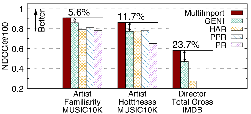
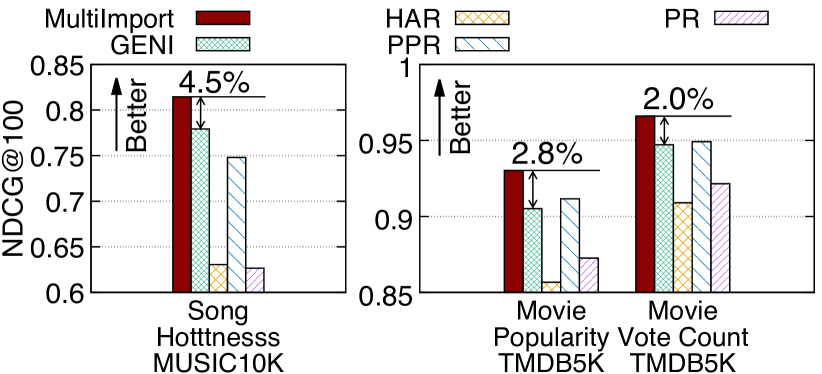
(c) Accuracy of estimated node importance on two KGs. (d) Input signal forecasting performance on two KGs.

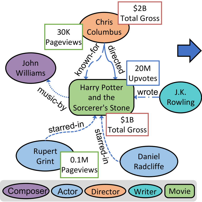
(a) A movie knowledge graph.

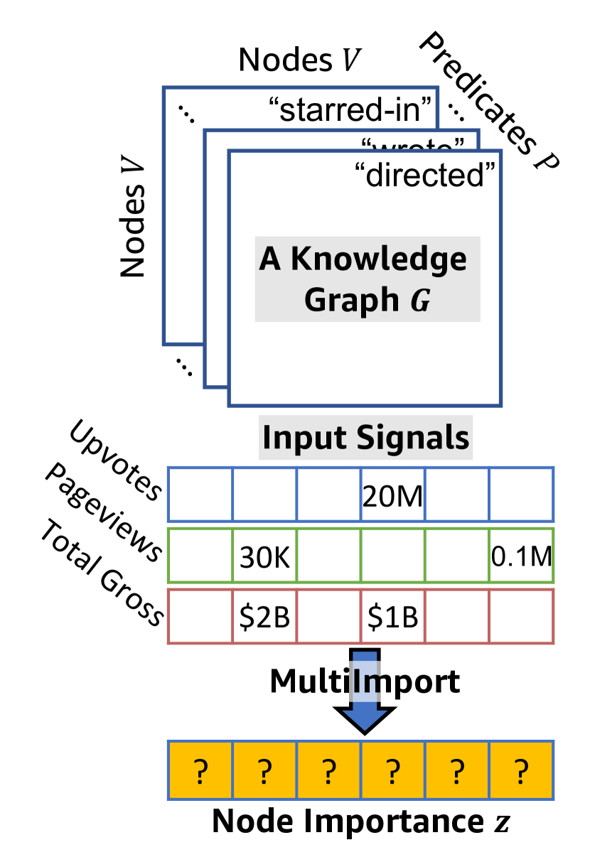
(b) Problem setup.

Figure 1. (a) A knowledge graph (KG) on a movie and related entities. Node color denotes an entity type and an edge type denotes the type of relation between entities. Rectangles represent input signals (e.g., total gross). Note that a single entity can have a variable number of input signals. (b) Given a KG and input signals, MultiImport infers the importance of all nodes. (c) MultiImport infers up to 23.7% more accurate node importance than the state-of-the-art method (GENI). (d) MultiImport achieves up to 4.5% higher forecasting results than baselines, with an NDCG@100 of 0.98 on tmdb5k. See Section 5 for details.

Real-world networks consist of several types of entities, interacting with each other via multiple types of relations. These complex and rich interactions between entities from diverse domains are abstracted by a knowledge graph (KG), which is a multi-relational graph where nodes are real-world entities or concepts, and edges denote the corresponding relation (also called predicate) between nodes. Given a KG, estimating node importance is a crucial task that has been studied extensively (Page et al., 1999; Haveliwala, 2002; Kleinberg, 1999; Tong et al., 2008; Li et al., 2012; Jung et al., 2017; Park et al., 2019a), as it enables a large number of applications such as recommendation, search, and ranking, to name a few.

A key challenge to achieve this goal lies in effectively using input from different sources. On the one hand, KGs represent how entities are related to each other. In particular, compared to the conventional graphs that make no distinction between edges, KGs provide abundant information as they comprise heterogeneous entities and predicates. For instance, consider the cross-domain KG on the movie “Harry Potter and the Sorcerer’s Stone” and related entities (Figure 1(a)), which consists of entities from various domains (e.g., “actor”, “composer”, and “movie”) and multiple relations (e.g., “directed” and “wrote”).

On the other hand, we can often obtain relevant data on the entities in a KG from external sources such as the World Wide Web. Among them, some are direct indicators of the importance or popularity of an entity as they capture how much time, money, or attention people have spent on it. The number of votes and pageviews are examples of such signals. We call this data that captures node importance input signal. A number of input signals are usually available for a KG, such as the total gross of movies in a movie KG, although they are often sparse and some are applicable to only specific types of entities, as illustrated in Figure 1(a).

Existing approaches for measuring node importance include random walk-based methods, such as PageRank (PR) (Page et al., 1999), Personalized PageRank (PPR) (Haveliwala, 2002), and HAR (Li et al., 2012), and more recent supervised techniques, such as GENI (Park et al., 2019a), which learn to estimate node importance. In the context of measuring entity importance in a multi-relational graph, these methods can be compared in terms of what type of input they can use, as Table 1 summarizes. While PR can consider only the graph structure, the development of more advanced random walk-based techniques enabled considering additional input. State-of-the-art results on this task have been achieved by GENI, which is built upon a supervised framework optimized to use both the KG and an external input signal.

However, all existing approaches can only consider up to one input signal, even though several signals are typically available from diverse sources. Also, while it is left to the users to decide which signal to use, no guideline has been provided. Importantly, by ignoring all other signals except for one, they lose information that can complement each other and provide more reliable and accurate evidence for node importance when used together.

In this paper, we present MultiImport, a supervised approach that makes an effective use of multiple input signals towards learning accurate and trustworthy node importance in a KG. Note that among different types of input listed in Table 1, input signals are the most direct and strongest indicator of node popularity. However, utilizing multiple signals raises several challenges that require careful design choices. First, given sparse, potentially overlapping, multiple input signals, it is not clear how unknown node importance can be inferred. Also, using all available signals may lead to worse results, when there exist conflicts among signals. Developing an effective graph-based estimator is another challenge to model the relation between node importance, input signals, and the KG.

To address these challenges, we model the task using a latent variable model and derive an effective learning objective. By adopting an iterative clustering-based training scheme, we handle those signals that may deteriorate the estimation quality. Also, we use predicate-aware, attentive graph neural networks (GNNs) to model the interactions among input signals and the KG. Our contributions are summarized as follows:

• Problem Formulation. We formulate the problem of inferring node importance in a KG from multiple input signals.

• Algorithm. We present MultiImport, a novel supervised method that effectively learns from multiple input signals by handling the aforementioned challenges.

• Effectiveness. We show the superiority of MultiImport using experiments on real-world KGs . Figures 1(c) and 1(d) show that MultiImport outperforms existing methods across multiple signals and KGs, achieving up to 23.7% higher NDCG@100 than the state of the art.

2. Background

Graph Neural Networks (GNNs) (Gilmer et al., 2017; Ying et al., 2018; Velickovic et al., 2018) are deep learning architectures for graph-structured data. GNNs consist of multiple layers, where each one updates the embeddings of each node by aggregating the embeddings from the neighborhood, and combining it with the current embeddings. How the $\ell$-th layer in GNNs computes the embeddings $\bm{\mathbf{h}}^{\ell}_{i}$ of node $i$ can be summarized as follows:

$$\bm{\mathbf{h}}^{\ell}_{i}\leftarrow\textsc{Combine}^{\ell}\left(\bm{\mathbf{h}}^{\ell-1}_{i},~{}\textsc{Aggregate}^{\ell}\left(\left\{\bm{\mathbf{h}}^{\ell-1}_{j}~{}\big{|}~{}j\in{\mathcal{N}}(i)\right\}\right)\right)$$

where ${\mathcal{N}}(i)$ denotes the neighbors of node $i$, $\textsc{Aggregate}^{\ell}$ is an operator that aggregates (e.g., averaging) the embeddings of neighbors, potentially after applying some form of transformation to them, and $\textsc{Combine}^{\ell}$ is an operator that merges the aggregated embeddings with the embeddings $\bm{\mathbf{h}}^{\ell-1}_{i}$ of node $i$. Different GNNs may use different definitions of ${\mathcal{N}}(i)$, $\textsc{Aggregate}^{\ell}(\cdot)$, and $\textsc{Combine}^{\ell}(\cdot)$.

3. Task Description

In this section, we present key concepts and the task description.

Knowledge Graph. A knowledge graph (KG) is a heterogeneous network with multiple types of entities and relations. As shown in Figure 1(b), a KG can be represented by a third-order tensor ${\bm{G}}\in\mathbb{R}^{|V|\times|P|\times|V|}$, in which a non-zero at $(s,\rho,o)$ indicates that a subject $s\in V$ is related to an object $o\in V$ via a predicate $\rho\in P$ where $V$ and $P$ are the sets of indices for entities and predicates, respectively. Real-world KGs, such as Freebase (Bollacker et al., 2008) and DBpedia (Lehmann et al., 2015), usually contain a large number of predicates. Also, two entities can be related via multiple predicates as in Figure 1(a).

Node Feature. Node-specific information is often available, and can be encoded in a vector of fixed length $F$. Examples include document embedding for the entity description, and more domain-specific features like motif gene sets from the Molecular Signatures Database (Subramanian et al., 2005). We use ${\bm{X}}\in\mathbb{R}^{|V|\times F}$ to denote all node features.

Node Importance. A node importance $z\in\mathbb{R}_{\geq 0}$ is a non-negative real number that represents the importance of an entity in a KG, with a higher value denoting a higher node importance. Node importance is a latent quantity, and thus not directly observable.

Input Signal. An input signal $S:V^{\prime}\rightarrow\mathbb{R}_{\geq 0}~{}(V^{\prime}\subseteq V)$ is a partial map between a node and a non-negative real number that represents the significance or popularity of the node. For entities in a KG, there are often several external data that could serve as an input signal. Examples of those signals include the number of copies sold (e.g., of books), the total gross of movies and directors, and the number of votes, reviews, and pageviews given for products. Note that they may highlight node popularity from different perspectives: e.g., number of clicks in the last one month (higher for trending movies) vs. total number of clicks so far (higher for classic movies). Also, some signals may be available only for some type of nodes (e.g., the number of tickets sold for movies).

In this work, we consider a set of ${M}$ input signals $\{S_{i}:{V_{i}^{\prime}}\rightarrow\mathbb{R}_{\geq 0}~{}|~{}V_{i}^{\prime}\subseteq V,i=1,\ldots,{M}\}$ where the signal domain $V_{i}^{\prime}$ might or might not overlap with each other. We note the following facts.

• Input signals can be in different scales. For example, while signal A ranges from 1 to 5, signal B could range from 0 to 100.

• Input signals often have high correlation as important nodes tend to have high values across different signals. However, signals may have a varying degree of correlation when signals capture different aspects of node importance or some involve more noise.

Task Description. Based on these concepts, our task of estimating node importance in a KG is summarized as follows (Figure 1(b) presents a pictorial overview):

Definition 3.1 (Node Importance Estimation).

Given a KG ${\bm{G}}\in\mathbb{R}^{|V|\times|P|\times|V|}$, node features ${\bm{X}}\in\mathbb{R}^{|V|\times F}$, and a set of ${M}$ input signals $\{S_{i}:{V_{i}^{\prime}}\rightarrow\mathbb{R}_{\geq 0}~{}|~{}V_{i}^{\prime}\subseteq V,i=1,\ldots,{M}\}$, where $V$ and $P$ denote the sets of indices of entities and predicates in ${\bm{G}}$, respectively, estimate the latent importance $z\in\mathbb{R}_{\geq 0}$ of every node in $V$.

4. Methods

Inferring node importance in a KG from multiple input signals requires addressing three major challenges.

1. Formulating learning objective. Given a KG and potentially overlapping signals, how can we infer latent node importance?

2. Handling rebel input signals. Given input signals that may possess different characteristics or involve more noise, how can we deal with potential conflicts and infer the node importance?

3. Effective graph-based estimation. How can we effectively model the relations between node importance, input signals, and the KG?

In this section, we present MultiImport that addresses the above challenges with the following ideas.

1. Modeling the task using a latent variable model enables capturing relations between node importance and input signals, and provides an optimization framework (Section 4.1).

2. Iterative clustering-based training handles rebel input signals, effectively inferring the node importance (Section 4.2).

3. Predicate-aware, attentive GNNs provide a powerful node importance estimator to infer graph-regularized node importance (Section 4.3).

The definition of symbols used in the paper is provided in Table 2.

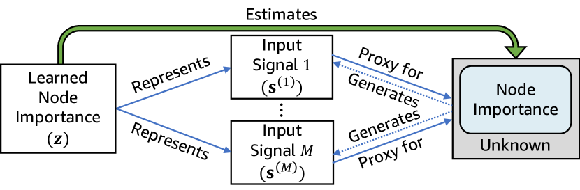
Figure 2. MultiImport estimates the latent node importance by learning to represent input signals, which are proxies for the unknown node importance.

4.1. Learning Objective

Given our task to infer node importance, one may consider using input signals directly as node features in supervised methods, as they provide useful cues on the significance of a node. However, since signals are partially observed, we will first need to fill in the missing values to use them as a node feature. Further, even if input signals are available for all nodes, with all signals treated as node features, it is not obvious how to infer node importance from them, as node importance is a latent value.

Given that node importance is unknown and cannot be directly observed, we assume that there is an underlying variable governing node importance, and observed input signals are generated by this variable with noise and possibly via non-linear transformations. Accordingly, we consider an input signal to be a partial indicator of latent node importance, and at the same time, to be a reasonably good proxy for the unknown node importance. Based on these assumptions, we approach our goal of estimating unknown node importance by learning to represent input signals. Figure 2 illustrates our assumptions on the relationship among the learned node importance, input signals, and node importance.

Notations. To formally define the learning objective, we introduce a few symbols. Let ${\bm{\mathcal{G}}}$ collectively denote the third-order tensor ${\bm{G}}$ representing the KG and the node features ${\bm{X}}$. We denote the number of dimensions of vector $\bm{\mathbf{v}}$ by $\dim(\bm{\mathbf{v}})$. Given ${M}$ observed input signals, let ${\bm{s}}^{(i)}$ denote a vector corresponding to the $i$-th signal, and ${\bm{S}}$ denote a set of ${M}$ signal vectors, i.e., ${\bm{S}}=\{{\bm{s}}^{(1)},{\bm{s}}^{(2)},\ldots,{\bm{s}}^{({M})}\}$. Let ${\bm{z}}\in\mathbb{R}^{|V|}$ denote a vector of estimated importance for all nodes. We use ${\bm{z}}^{(i)}$ to refer to the vector of estimated importance of those nodes for which signal $i$ is available. Thus, $\dim({\bm{z}}^{(i)})$ equals $\dim({\bm{s}}^{(i)})$. Since signals are partially observable, we have that $\dim({\bm{s}}^{(i)})=\dim({\bm{z}}^{(i)})\leq|V|=\dim({\bm{z}})$. To denote the $j$-th value of a signal or estimated importance, we use a subscript, e.g., $s^{(i)}_{j}$ and $z^{(i)}_{j}$.

Maximum a Posteriori Learning. Our goal can be summarized as learning an estimator $f(\cdot)$ that produces estimated importance ${\bm{z}}$ for all nodes in the KG. Specifically, as we consider a graph-based estimator with learnable parameters, the estimation by $f(\cdot)$ is determined by the given KG ${\bm{\mathcal{G}}}$ and its learnable parameters ${\bm{\theta}}$. In other words, we have:

(1) $${\bm{z}}=f({\bm{\mathcal{G}}},{\bm{\theta}}).$$

In order to optimize $f(\cdot)$, we aim to maximize the posterior probability of model parameters ${\bm{\theta}}$ given that we have observed the KG ${\bm{\mathcal{G}}}$ and input signals ${\bm{S}}$:

(2) $$\max p({\bm{\theta}}|{\bm{\mathcal{G}}},{\bm{S}}).$$

By the Bayes’ theorem, this is equivalent to maximizing:

(3) $$p({\bm{\theta}}|{\bm{\mathcal{G}}},{\bm{S}})=\frac{p({\bm{\mathcal{G}}},{\bm{S}}|{\bm{\theta}})\,p({\bm{\theta}})}{p({\bm{\mathcal{G}}},{\bm{S}})}\propto p({\bm{\theta}})\,p({\bm{\mathcal{G}}}|{\bm{\theta}})\,p({\bm{S}}|{\bm{\mathcal{G}}},{\bm{\theta}}).$$

The first term $p({\bm{\theta}})$ in Equation 3 represents the prior probability of the model parameters ${\bm{\theta}}$, which we assume to be a Gaussian distribution with zero mean and an isotropic covariance:

(4) $$p(\bm{\theta})=\mathcal{N}(\bm{\theta}|\bm{\mathbf{0}},\lambda^{-1}\bm{\mathbf{{I}}}).$$

The second term $p({\bm{\mathcal{G}}}|{\bm{\theta}})$ in Equation 3 is the likelihood of the observed KG ${\bm{\mathcal{G}}}$ given ${\bm{\theta}}$. As we later discuss in Section 4.3, given features $\bm{\mathbf{x}}_{i}$ of node $i$, MultiImport embeds node $i$ in an intermediate low-dimensional space by projecting $\bm{\mathbf{x}}_{i}$ using a learnable function $g(\cdot)$. Let $(s,\rho,o)$ denote a subject-predicate-object triple in the KG. Using factorization-based KG embeddings (Wang et al., 2017), we model the observed triple $(s,\rho,o)$ as a diagonal bilinear interaction between node embeddings $g(\bm{\mathbf{x}}_{s})$, $g(\bm{\mathbf{x}}_{o})$ and the learnable predicate embedding $\bm{\mathbf{w}}_{\rho}$ with normally distributed errors. Specifically,

(5) $$p({\bm{\mathcal{G}}}|{\bm{\theta}}) =\prod_{(s,\rho,o)\in{\bm{\mathcal{G}}}}p((s,\rho,o)|{\bm{\theta}})$$

(6) $$=\prod_{(s,\rho,o)\in{\bm{\mathcal{G}}}}\mathcal{N}\left(g(\bm{\mathbf{x}}_{s})^{\intercal}\mathop{\mathrm{diag}}(\bm{\mathbf{w}}_{\rho})~{}g(\bm{\mathbf{x}}_{o})\Big{|}1,\nu^{-1}\right)$$

where $\mathop{\mathrm{diag}}(\bm{\mathbf{w}}_{\rho})$ denotes a diagonal matrix where the diagonal entries are given by $\bm{\mathbf{w}}_{\rho}$. This term can also be seen as an assumption on the homophily between neighboring nodes in the space represented by node embedding $g(\cdot)$ and predicate $\rho$.

The third term $p({\bm{S}}|{\bm{\mathcal{G}}},{\bm{\theta}})$ of Equation 3 is the likelihood of observed input signals ${\bm{S}}$ given the KG ${\bm{\mathcal{G}}}$ and model parameters ${\bm{\theta}}$. Given ${M}$ signals, we assume that they are conditionally independent. Accordingly, we have that:

(7) $$p({\bm{S}}|{\bm{\mathcal{G}}},{\bm{\theta}})=p({\bm{s}}^{(1)}|{\bm{\mathcal{G}}},{\bm{\theta}})\cdot\ldots\cdot p({\bm{s}}^{({M})}|{\bm{\mathcal{G}}},{\bm{\theta}}).$$

Recall that ${\bm{z}}$ is a function of ${\bm{\mathcal{G}}}$ and ${\bm{\theta}}$, or in other words, ${\bm{\mathcal{G}}}$ and ${\bm{\theta}}$ fully determine ${\bm{z}}$, and input signals can be partially observed (i.e., $\dim({\bm{s}}^{(i)})$ may not equal $\dim({\bm{z}})$). Equation 7 can be expressed in terms of input signals and the corresponding estimated importance:

(8) $$p({\bm{S}}|{\bm{\mathcal{G}}},{\bm{\theta}})\propto p({\bm{s}}^{(1)}|{\bm{z}}^{(1)})\cdot\ldots\cdot p({\bm{s}}^{({M})}|{\bm{z}}^{({M})})$$

in which the log-likelihood $\log p({\bm{s}}^{(i)}|{\bm{z}}^{(i)})$ of observing signal ${\bm{s}}^{(i)}$ given ${\bm{z}}^{(i)}$ is proportional to:

(9) $$\log p({\bm{s}}^{(i)}|{\bm{z}}^{(i)})\propto\log\prod_{j=1}^{\dim({\bm{s}}^{(i)})}{p(z^{(i)}_{j})}^{p(s^{(i)}_{j})}=\sum_{j=1}^{\dim({\bm{s}}^{(i)})}{p(s^{(i)}_{j})}\log{p(z^{(i)}_{j})}.$$

Note that taking a negative of Equation 9 leads to the cross entropy.

Table 2. Table of symbols.

Symbol Definition ${\bm{\mathcal{G}}}$ knowledge graph with node features $V,P$ set of indices of nodes and predicates in a KG $\bm{\mathbf{x}}_{i},{\bm{X}}$ feature vector of node $i$, and a matrix of all node features ${\bm{\theta}}$ learnable parameters of the node importance estimator $f(\cdot)$ ${M}$ number of input signals ${\bm{s}}^{(i)}$ a vector of $i$-th observed input signal ${\bm{S}}$ a set of ${M}$ input signals, i.e., ${\bm{S}}=\{{\bm{s}}^{(1)},{\bm{s}}^{(2)},\ldots,{\bm{s}}^{({M})}\}$ ${\bm{z}}$ a vector of estimated importance of all nodes ${\bm{z}}^{(i)}$ a vector of estimated importance of those nodes with signal $i$ $\dim(\bm{\mathbf{z}})$ number of dimensions of vector $\bm{\mathbf{z}}$ $\mathop{\mathrm{diag}}(\bm{\mathbf{w}})$ a diagonal matrix whose diagonal entries are given by vector $\bm{\mathbf{w}}$ ${\mathcal{N}}(i)$ neighboring edges of node $i$ $h^{\ell}_{i}$ importance of node $i$ estimated by the $\ell$-th layer in the GNN $h^{*}_{i}$ final estimated importance of node $i$ by the GNN (i.e., $z_{i}=h^{*}_{i}$) $\omega^{\ell}_{ij}$ node $i$’s attention on the $m$-th edge from node $j$ in layer $\ell$ $\pi(\rho_{ij}^{m})$ learnable predicate embedding of $m$-th edge between nodes $i$ and $j$

With respect to the probability $p({\bm{s}}^{(i)})$ of observing signal ${\bm{s}}^{(i)}$, we consider two things. First, input signals can be in different scales. Since signals are obtained from diverse sources, their values could be in different scales and units, and thus may not be directly comparable (e.g., # clicks vs. dwell time vs. the total revenue in dollars). Second, for most downstream applications of node importance, the rank of each entity’s importance matters much more than the raw value itself. In light of these observations, we consider the probability of observing a signal vector in terms of ranking.

To do so, once we obtain a list of entity rankings from the signal vector, we need a probability model that measures the likelihood of the ranked list. Permutation probability (Cao et al., 2007) is one such model, in which the likelihood of a ranked list is defined with respect to a given permutation of the list, such that the permutation which corresponds to sorting entities according to their ranking is most likely to be observed. In our setting, however, this model is not feasible since there are $O(|V|!)$ permutations to be considered. Instead, we use a tractable approximation of it called top one probability. Given signal ${\bm{s}}^{(i)}$, the top one probability $p(s^{(i)}_{j})$ of $j$-th entity in ${\bm{s}}^{(i)}$ represents the probability of that entity to be ranked at the top of the list given the signal values of other entities, and is defined as:

(10) $$p(s^{(i)}_{j})=\frac{\phi(s^{(i)}_{j})}{\sum_{k=1}^{\dim({\bm{s}}^{(i)})}\phi(s^{(i)}_{k})}=\frac{\exp(s^{(i)}_{j})}{\sum_{k=1}^{\dim({\bm{s}}^{(i)})}\exp(s^{(i)}_{k})}.$$

Here, $\phi(\cdot)$ is a strictly increasing positive function, which we define to be an exponential function. Similarly, given model estimation ${\bm{z}}^{(i)}$, the top one probability $p(z^{(i)}_{j})$ of $j$-th entity in ${\bm{z}}^{(i)}$ is computed as:

(11) $$p(z^{(i)}_{j})=\frac{\exp(z^{(i)}_{j})}{\sum_{k=1}^{\dim({\bm{z}}^{(i)})}\exp(z^{(i)}_{k})}.$$

Taking a negative logarithm of our posterior in Equation 3 and plugging in Equations 4, 8, 6 and 9, we get the following loss:

where $p(s^{(i)}_{j})$ and $p(z^{(i)}_{j})$ are given by Equations 10 and 11.

4.2. Handling Rebel Input Signals

In Section 4.1, MultiImport infers node importance from all ${M}$ input signals. This is based on the assumption that the given signals have been generated by a common hidden variable as depicted in Figure 2, that is, input signals are homogeneous and a high correlation exists among them. However, some signals (which we call rebel signals) may exhibit a low correlation with the others when they possess different characteristics from others, or involve more noise. As a result, when given multiple signals where some are weakly correlated with others, learning from all of them leads to a worse estimator due to the violation of our modeling assumption.

To effectively infer node importance from multiple signals while handling rebel signals, we adopt an iterative clustering-based training, where closely related input signals are put into the same cluster and our estimator is trained using not all the given signals, but only those in the same cluster. To do so, we need to be able to measure the relatedness of input signals. Again, considering that signals can be in different scales and ranks are important for downstream applications, we compare a pair of signals in terms of the Spearman correlation coefficient, a well-known rank correlation measure.

However, comparing input signals is not always possible, since they can be disjoint as signals are partially observable. To handle this, MultiImport (a) initially assigns ${M}$ signals to their own cluster, (b) separately infers node importance from each one, (c) do a pairwise comparison between observed and inferred values, and (d) merges clusters by applying existing clustering algorithms, such as DBSCAN (Ester et al., 1996), on the pairwise signal similarity. With the resulting clusters, we repeat the same process again until there is no change in the clustering. This is because learning from an enlarged cluster can lead to a higher modeling accuracy, as we show in Section 5.4. If there is enough overlap between signals’ observed values, we may omit step (b), and compute their similarity directly from observed values in step (c). These steps are illustrated in Figure 3, and Algorithm 1 gives our learning algorithm.

Given multiple signals, our focus is to infer a single number for each node, which represents the major aspect of node importance, as supported by the signals and relevant to downstream applications. This requires sorting the final clusters based on their priority. Examples of such priority policy $\pi$ include: (1) cluster size (prefer a cluster with a larger number of signals); (2) cluster quality (prefer a cluster with a higher reconstruction accuracy); (3) signal preference (prefer a cluster with signals that are important for the given application). In experiments, we use cluster size as our priority.

Incremental Learning. Our approach naturally lends itself to incremental learning settings where new signals are added after the model training. As in the initial training phase, new signals are first put into their own cluster, and MultiImport merges them with existing clusters based on the similarity of inferred importance.

4.3. Graph Neural Networks for
Node Importance Estimation

Given this optimization framework, we now present a supervised estimator $f(\cdot)$ that can model complex relations among input signals and the information of the KG. In MultiImport, we utilize GNNs, which have been shown to be a powerful model for learning on a graph. We adopt and improve upon the recent development of GNNs, such as the dynamic neighborhood aggregation via an attention mechanism, by making extensions and simplifications.

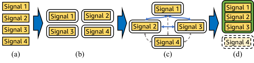
Figure 3. MultiImport identifies similar signals (those in the green cluster), and infers node importance from them. See text for details of steps (a) to (d).

Input: knowledge graph ${\bm{\mathcal{G}}}$, input signals ${\bm{S}}$, merge threshold $t$, priority policy $\pi$.

Output: estimated node importance.

1

2repeat

3       Assign input signals without cluster membership (e.g., newly added signals) to their own cluster, if any

4      

5      foreach cluster $c$ do

6             Infer node importance by training an estimator $f_{c}(\cdot)$ with the loss function in Equation 12

7      

8      Merge those clusters whose similarity is greater than threshold $t$

9until there is no change in the clustering

return node importance inferred from the cluster that has the highest priority according to the policy $\pi$

Algorithm 1 Learning algorithm

MultiImport first projects features $\bm{\mathbf{x}}_{i}$ of node $i$ to a low-dimensional space using a learnable function $g(\cdot)$. Let $\bm{\mathbf{x}}^{\prime}_{i}=g(\bm{\mathbf{x}}_{i})$. As discussed in Section 4.1, MultiImport allows assuming homophily among neighboring nodes in this embedding space. Given these intermediate node embeddings, our estimator further transforms them into one dimensional embedding to directly represent nodes by their importance. To do so, MultiImport uses another learnable function $g^{\prime}(\cdot)$. In other words, MultiImport represents node $i$ as $h^{0}_{i}\in\mathbb{R}$ in the space of node importance such that ${h^{0}_{i}=g^{\prime}(\bm{\mathbf{x}}^{\prime}_{i})}$. Note that both $g(\cdot)$ and $g^{\prime}(\cdot)$ are learnable functions, and can be a simple linear transformation or multi-layer neural networks.

Then, given $h^{0}_{i}$ for all $i$, we apply attentive GNNs to it on the given KG to obtain graph-regularized node importance such that the estimated importance smoothly changes with respect to the KG in a predicate-aware manner. MultiImport is a multi-layer GNN with $L$ layers. The $\ell$-th layer performs a weighted aggregation of the node importance estimated by the $(\ell\!-\!1)$-th layer from the neighborhood ${\mathcal{N}}(i)$ to produce a new estimation $h^{\ell}_{i}$ for node $i$:

(13) $$h^{\ell}_{i} =\sum_{(j,m)\in{\mathcal{N}}(i)}\omega^{\ell}_{(i,j,m)}~{}h^{\ell-1}_{j}$$

Although attentive GNNs usually compute the attention weight for neighboring nodes assuming simple graphs, KGs are directed graphs with parallel edges. Therefore, instead of node-level attention, we compute edge-level attention weights, which enables making a distinction among edges between two nodes. We define ${\mathcal{N}}(i)$ to be a set of neighboring edges of node $i$ such that $(j,m)\in{\mathcal{N}}(i)$ if there exists an $m$-th edge between nodes $i$ and $j$ (under some edge ordering). The weight $\omega^{\ell}_{(i,j,m)}$ of the edge $(j,m)\in{\mathcal{N}}(i)$ is then computed using a predicate-aware attention parameterized by a weight vector $\bm{\mathbf{a}}_{\ell}$:

(14) $$\omega^{\ell}_{(i,j,m)}\! =\!\frac{\exp\left(\text{LeakyReLU}\left(\bm{\mathbf{a}}_{\ell}^{\intercal}\left[h^{\ell-1}_{i}\big{|}\big{|}\pi(\rho_{ij}^{m})\big{|}\big{|}h^{\ell-1}_{j}\right]\right)\right)}{\sum_{(k,n)\in{\mathcal{N}}(i)}\exp\left(\text{LeakyReLU}\left(\bm{\mathbf{a}}_{\ell}^{\intercal}\left[h^{\ell-1}_{i}\big{|}\big{|}\pi(\rho_{ik}^{n})\big{|}\big{|}h^{\ell-1}_{k}\right]\right)\right)}$$

where ${\rho}_{ij}^{m}$ denotes the predicate type of $m$-th edge between nodes $i$ and $j$, $\pi(\cdot)$ is a learnable function that maps a predicate type to its embedding (i.e., $\pi(\rho_{ij}^{m})$ is the embedding of the predicate of the $m$-th edge between nodes $i$ and $j$), and $||$ is a concatenation operator. Motivated by GENI, we generate the final estimation $h^{*}_{i}$ for node $i$ by making a centrality-based adjustment to the estimation $h^{L}_{i}$ made by the final layer $L$, where in-degree $d_{i}$ of node $i$ is used to define its centrality $c_{i}$:

(15) $$\begin{split}c_{i}&=\alpha\cdot\log(d_{i}+\epsilon)+\beta\\ h^{*}_{i}&=\text{ReLU}\left(c_{i}\cdot h^{L}_{i}\right)\end{split}$$

where $\alpha$ and $\beta$ are learnable parameters and $\epsilon$ is a small positive value. In summary, the final estimated node importance $\bm{\mathbf{z}}$ is produced as follows:

(16) $${\bm{z}}=f({\bm{\mathcal{G}}},{\bm{\theta}})=[h^{*}_{1},\ldots,h^{*}_{|V|}]^{\intercal}.$$

5. Experiments

In this section, we address the following questions.

1. Accuracy. How consistent is estimated node importance with input signals? In particular, how does the estimation performance change when multiple input signals are considered?

2. Use in downstream tasks. How useful is the estimated importance for downstream tasks?

3. Handling rebel signals. How does a rebel signal affect the performance, and how well does our method handle it?

After describing datasets, evaluation plans, and baselines in Sections 5.1, 5.2 and 5.3, we address the above questions in Sections 5.4, 5.5 and 5.6. Experimental settings are presented in Appendix A.

5.1. Dataset Description

We used four publicly available real-world KGs that have different characteristics, and were used in a previous study on node importance estimation (Park et al., 2019a). We constructed these datasets following the description in (Park et al., 2019a). Below we give a brief description of these KGs. Statistics of these data are given in Table 3, and the list of available input signals in each KG is provided in Table 4.

fb15k (Bordes et al., 2013) is a KG sampled from the Freebase knowledge base (Bollacker et al., 2008), which consists of general knowledge harvested from many sources, and compiled by collaborative efforts. fb15k is much denser and contains a much larger number of predicates than other KGs.

music10k is a music KG representing the relation between songs, artists, and albums. music10k is constructed from a subset of the Million Song Dataset, and it provides three input signals called “song hotttnesss”, “artist hotttnesss”, and “artist familiarity”, which are popularity scores computed by considering several relevant data such as playback count.

tmdb5k is a movie KG representing relations among movie-related entities such as movies, actors, directors, crews, casts, and companies. tmdb5k is constructed from the TMDb 5000 datasets, and contains several signals including the “popularity” score computed by considering relevant statistics like the number of votes.

imdb is a movie KG constructed from the daily snapshot of the IMDb dataset on movies and related entities, e.g., genres, directors, casts, and crews. imdb is the largest KG among the four KGs. As IMDb dataset provides only one input signal (# votes), we collected popularity signal from TMDb for 5% of the movies in imdb.

Table 3. Real-world KGs used in our evaluation. These KGs vary in different aspects, such as the size and number of predicates. SCC: Strongly connected component.

Name # Nodes # Edges # Predicates # SCCs fb15k 14,951 592,213 1,345 9 music10k 24,830 71,846 10 130 tmdb5k 123,906 532,058 22 15 imdb 1,567,045 14,067,776 28 1

Table 4. Input signals in real-world KGs. The percentage of nodes covered by each signal is given in the parentheses.

Name Type Input Signals fb15k Generic # Pageviews, # total edits, and # page watchers on Wikipedia (all 94%) music10k Artist Artist hotttnesss (14%) and artist familiarity (16%) Song Song hotttnesss (17%) tmdb5k Movie Popularity, revenue, budget, and vote count (all 4%) Director Box office grosses for top 200 directors imdb Movie # Votes (14%) and popularity (from TMDb, 5%) Director Box office grosses for top 200 directors

Table 5. MultiImport estimates node importance more accurately than baselines, and using additional signals improves the accuracy. MultiImport-1 is the same as MultiImport except that it used only one signal denoted with an asterisk (*). Methods that can use only one input signal also used the one marked with an asterisk (*). The best result is in bold and in dark gray. The second best result is underlined and in light gray. TR: Training. ID: In-Domain. OOD: Out-Of-Domain.

	fb15k			music10k
Method	# Page Watchers* (Generic, TR, ID)	# Total Edits (Generic, TR, ID)	# Pageviews (Generic, ID)	Familiarity* (Artist, TR, ID)	Hotttnesss (Artist, TR, ID)	Hotttnesss (Song, OOD)
PR	0.7747 $\pm$ 0.02	0.8579 $\pm$ 0.00	0.8441 $\pm$ 0.00	0.7788 $\pm$ 0.01	0.6520 $\pm$ 0.00	0.4846 $\pm$ 0.00
PPR	0.7810 $\pm$ 0.02	0.8604 $\pm$ 0.00	0.8450 $\pm$ 0.00	0.8090 $\pm$ 0.01	0.7823 $\pm$ 0.01	0.6422 $\pm$ 0.02
HAR	0.7625 $\pm$ 0.01	0.9080 $\pm$ 0.00	0.8732 $\pm$ 0.00	0.7905 $\pm$ 0.01	0.7751 $\pm$ 0.01	0.6377 $\pm$ 0.01
GENI	0.8548 $\pm$ 0.02	0.8787 $\pm$ 0.04	0.8464 $\pm$ 0.03	0.8603 $\pm$ 0.01	0.7727 $\pm$ 0.02	0.6804 $\pm$ 0.01
MultiImport-1	0.8879 $\pm$ 0.02	0.9250 $\pm$ 0.03	0.8863 $\pm$ 0.03	0.8839 $\pm$ 0.01	0.8046 $\pm$ 0.02	0.7109 $\pm$ 0.02
MultiImport	0.9150 $\pm$ 0.01	0.9498 $\pm$ 0.01	0.9066 $\pm$ 0.01	0.9083 $\pm$ 0.00	0.8633 $\pm$ 0.02	0.7173 $\pm$ 0.01

space

	tmdb5k				imdb
Method	Popularity* (Movie, TR, ID)	Vote Count (Movie, TR, ID)	Revenue (Movie, ID)	Total Gross (Director, OOD)	# Votes* (Movie, TR, ID)	Popularity (Movie, TR, ID)	Total Gross (Director, OOD)
PR	0.8294 $\pm$ 0.02	0.8482 $\pm$ 0.00	0.9009 $\pm$ 0.00	0.8829 $\pm$ 0.00	0.7927 $\pm$ 0.02	0.7019 $\pm$ 0.00	0.0000 $\pm$ 0.00
PPR	0.8585 $\pm$ 0.01	0.9133 $\pm$ 0.01	0.9535 $\pm$ 0.00	0.8691 $\pm$ 0.02	0.7927 $\pm$ 0.02	0.7169 $\pm$ 0.01	0.0000 $\pm$ 0.00
HAR	0.8131 $\pm$ 0.02	0.9350 $\pm$ 0.00	0.9537 $\pm$ 0.00	0.9298 $\pm$ 0.01	0.7976 $\pm$ 0.02	0.7671 $\pm$ 0.00	0.2735 $\pm$ 0.03
GENI	0.9055 $\pm$ 0.02	0.9367 $\pm$ 0.00	0.9646 $\pm$ 0.00	0.9398 $\pm$ 0.00	0.9367 $\pm$ 0.00	0.7079 $\pm$ 0.01	0.4703 $\pm$ 0.02
MultiImport-1	0.9075 $\pm$ 0.02	0.9555 $\pm$ 0.00	0.9650 $\pm$ 0.00	0.9497 $\pm$ 0.00	0.9493 $\pm$ 0.00	0.7581 $\pm$ 0.01	0.5607 $\pm$ 0.01
MultiImport	0.9302 $\pm$ 0.01	0.9536 $\pm$ 0.00	0.9716 $\pm$ 0.00	0.9558 $\pm$ 0.00	0.9542 $\pm$ 0.01	0.8444 $\pm$ 0.02	0.5819 $\pm$ 0.03

5.2. Performance Evaluation

For evaluation, we use normalized discounted cumulative gain (NDCG), which is a widely used metric for relevance ranking problems. Given a list of nodes for which we have the estimated importance and the ground truth scores, we sort the list by the estimated importance, and consider the ground truth signal value at position $i$ (denoted by $r_{i}$) to compute the discounted cumulative gain at position $k$ ($DCG@k$) as follows:

$$DCG@k=\sum_{i=1}^{k}\frac{r_{i}}{\log_{2}(i+1)}.$$

The gain is accumulated from the top to the bottom of the list, and gets reduced at lower positions due to the logarithmic reduction factor. An ideal DCG at rank position $k$ ($IDCG@k$) can be obtained by sorting nodes by their ground truth values, and computing $DCG@k$ for this ordered list. Normalized DCG at position $k$ ($NDCG@k$) ranges from 0 to 1, and is defined as:

$$NDCG@k=\frac{DCG@k}{IDCG@k}$$

with higher values indicating a better ranking quality.

In computing NDCG, we consider all entities if the input signal is generic and applies to all entity types as in fb15k. Otherwise, we consider only those entities of the type for which the ground truth signal applies. For instance, to compute NDCG with respect to movie popularity, we only consider movies. In general, we compute NDCG over those entities that have ground truth values. An exception is the director signal, which is limited to the top 200 directors based on their worldwide box office grosses. When computing NDCG for the director signal, we consider all director entities, and assume the ground truth of the directors to be 0 if they are outside the top 200 list. In our experiments, we report NDCG@100; using different values for the threshold $k$ yielded similar results.

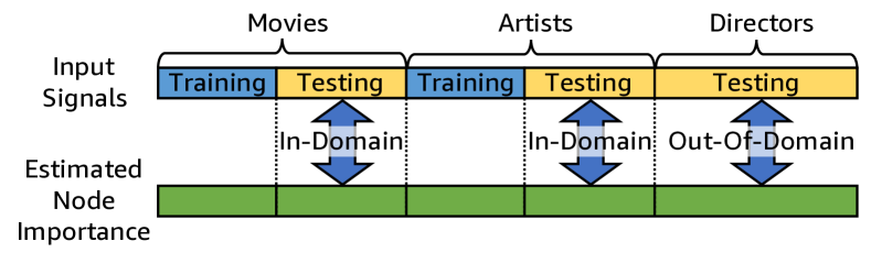
Figure 4. In- and out-of-domain evaluation where three input signals are given and two are used for training.

Generalization. In order to evaluate the generalization ability of each method, we perform 5-fold cross validation where 80% of the input signals are used for training, while the remaining 20% are used for testing. Similar results were observed with different number of folds. Also, since input signals often apply to a specific type of nodes (e.g., directors), we also consider how well a method generalizes to the nodes of unseen types. Consider Figure 4 for an example. Given input signals on movies, artists, and directors, movie and artist signals are used for both training and testing, while the director signal is used for testing alone. Here we call an evaluation on movies and artists in-domain as training involved input signals on these types of nodes, and an evaluation on directors out-of-domain since training used no input signal on this type. It is desirable to achieve a higher accuracy in both criteria.

5.3. Baselines

We use the following baselines: PageRank (PR) (Page et al., 1999), Personalized PageRank (PPR) (Haveliwala, 2002), HAR (Li et al., 2012), and GENI (Park et al., 2019a). PR, PPR, and HAR are representative random walk-based algorithms for measuring node importance. GENI is a supervised method that achieved the state-of-the-art result. We omitted results from other supervised algorithms, including linear regression, random forests, dense neural networks, and other GNNs, such as GAT (Velickovic et al., 2018) and GCN (Kipf and Welling, 2017), as GENI has been shown to outperform them in our experiments.

5.4. Q1. Accuracy

The quality of estimated node importance can be measured by how well it correlates with the observed signals. That is, accurately estimated node importance ${\bm{z}}$ should strongly correlate with input signals. We measure the degree of correlation between the estimation ${\bm{z}}$ and input signals using NDCG. In Table 5, we report NDCG@100 of estimated node importance with respect to each signal in our four KGs.

In the table, only those signals marked with TR were used for training. For baselines that can accept at most one input signal (PPR, HAR, and GENI), we used the signal marked with an asterisk (*) as the training signal. MultiImport-1 is identical to MultiImport except that only one signal (marked with *) is used for training.

Overall, MultiImport consistently outperformed baselines across all signals on four datasets, in terms of both in-domain (ID) and out-of-domain (OOD) evaluation. Note that MultiImport inferred node importance by learning from the given multiple signals. A comparison between MultiImport and MultiImport-1 shows that learning from multiple input signals led to a performance improvement of up to 11%. Even if the training signals were given for the same type of entities (e.g., artists or movies), considering multiple signals also improved the performance on OOD entities (e.g., songs or directors). While GENI performed better than random walk-based methods in most cases, it was outperformed by MultiImport due to its inability to consider multiple signals.

Table 6. MultiImport achieves the best signal prediction results (marked in bold and in dark gray), where we use input signals and estimated node importance as input features to predict another input signal. In only one exception, MultiImport achieves the second best result (underlined and in light gray). $\bm{z}_{m}$ denotes node importance estimated by method $m$.

   

(a) Predicting “budget” on tmdb5k by using popularity ($\bm{p}$), vote count ($\bm{v}$) and estimated node importance ($\bm{z}$) as features.

Input Features	NDCG@10	NDCG@100
$\bm{p},\bm{v}$	0.8296 $\pm$ 0.09	0.8176 $\pm$ 0.00
$\bm{p},\bm{v},\bm{z}_{\textsc{PR}}$	0.8700 $\pm$ 0.06	0.8260 $\pm$ 0.00
$\bm{p},\bm{v},\bm{z}_{\textsc{PPR}}$	0.8602 $\pm$ 0.07	0.8312 $\pm$ 0.01
$\bm{p},\bm{v},\bm{z}_{\textsc{HAR}}$	0.8341 $\pm$ 0.08	0.8062 $\pm$ 0.02
$\bm{p},\bm{v},\bm{z}_{\textsc{GENI}}$	0.8791 $\pm$ 0.06	0.8740 $\pm$ 0.01
$\bm{p},\bm{v},\bm{z}_{\textbf{{Multi\-Import}}}$	0.8930 $\pm$ 0.07	0.8757 $\pm$ 0.00

(b) Predicting “artist hotttnesss” on music10k by using artist familiarity ($\bm{f}$) and estimated node importance ($\bm{z}$) as features.

Input Features	NDCG@10	NDCG@100
$\bm{f}$	0.3727 $\pm$ 0.12	0.5751 $\pm$ 0.05
$\bm{f},\bm{z}_{\textsc{PR}}$	0.4092 $\pm$ 0.03	0.5839 $\pm$ 0.01
$\bm{f},\bm{z}_{\textsc{PPR}}$	0.3685 $\pm$ 0.12	0.5727 $\pm$ 0.05
$\bm{f},\bm{z}_{\textsc{HAR}}$	0.3727 $\pm$ 0.12	0.5751 $\pm$ 0.05
$\bm{f},\bm{z}_{\textsc{GENI}}$	0.3484 $\pm$ 0.15	0.5650 $\pm$ 0.06
$\bm{f},\bm{z}_{\textbf{{Multi\-Import}}}$	0.4186 $\pm$ 0.06	0.5886 $\pm$ 0.00

(c) Predicting “# page watchers” on fb15k by using # num pageviews ($\bm{p}$), # num total edits ($\bm{e}$) and estimated node importance ($\bm{z}$) as features.

Input Features	NDCG@10	NDCG@100
$\bm{p},\bm{e}$	0.8681 $\pm$ 0.01	0.8859 $\pm$ 0.02
$\bm{p},\bm{e},\bm{z}_{\textsc{PR}}$	0.9010 $\pm$ 0.01	0.8975 $\pm$ 0.02
$\bm{p},\bm{e},\bm{z}_{\textsc{PPR}}$	0.9010 $\pm$ 0.01	0.8975 $\pm$ 0.02
$\bm{p},\bm{e},\bm{z}_{\textsc{HAR}}$	0.9052 $\pm$ 0.00	0.8945 $\pm$ 0.02
$\bm{p},\bm{e},\bm{z}_{\textsc{GENI}}$	0.8884 $\pm$ 0.00	0.9076 $\pm$ 0.02
$\bm{p},\bm{e},\bm{z}_{\textbf{{Multi\-Import}}}$	0.9084 $\pm$ 0.00	0.9062 $\pm$ 0.02

Table 7. MultiImport outperforms all baselines in forecasting signals. TR denotes the signals used for training MultiImport; baselines were trained with the one marked with an asterisk (*). The bottom table shows how data was split.

	tmdb5k			music10k
Method	Popularity* (Movie, TR) NDCG@100	Vote Count (Movie, TR) NDCG@100	Budget (Movie) NDCG@100	Hotttnesss* (Song, TR) NDCG@100
PR	0.8726	0.9215	0.9294	0.6266
PPR	0.9116	0.9492	0.9640	0.7480
HAR	0.8567	0.9090	0.9265	0.6306
GENI	0.9051	0.9472	0.9647	0.7792
MultiImport	0.9303	0.9660	0.9829	0.8145

space

Dataset	Training (# Entities)	Testing (# Entities)
tmdb5k	Movies released until 2013 (4243)	Movies released from 2014 (559)
music10k	Songs released until 2005 (1961)	Songs released from 2006 (751)

5.5. Q2. Use in Downstream Tasks

Estimated importance ${\bm{z}}$ can be viewed as a summary of KG nodes in terms of input signals. This summary can be used as a feature in downstream applications. In this section, we evaluate how useful MultiImport’s estimation ${\bm{z}}$ is in downstream signal prediction and forecasting tasks, as opposed to the estimation learned by baselines.

Signal Prediction. The signal prediction task is to predict some input signal ${\bm{s}}^{(i)}$ using a machine learning model (M) that uses other input signals ${\bm{s}}^{(1)},\ldots,{\bm{s}}^{(i-1)}$ and the estimated node importance ${\bm{z}}$ as input features. Here ${\bm{z}}$ can be generated by different methods. Each method uses only ${\bm{s}}^{(1)},\ldots,{\bm{s}}^{(i-1)}$, and no other input signals (i.e., ${\bm{s}}^{(i)}$ is not available during generation of ${\bm{z}}$). Once ${\bm{z}}$ is obtained, we compare the performance of M when the input features consist of only ${\bm{s}}^{(1)},\ldots,{\bm{s}}^{(i-1)}$ vs. when they are composed of both ${\bm{s}}^{(1)},\ldots,{\bm{s}}^{(i-1)}$ and ${\bm{z}}$. Also, we compare the prediction performance of M as we use ${\bm{z}}$ obtained with different methods. The motivation for this signal prediction test is that estimated importance can be considered as de-noising compression of input signals. Thus a high-quality estimate of importance should be a useful input feature for downstream signal prediction model. We used a linear regression model as our M and optimized it using the loss shown in Equation 12 (without the second term), using input signals from tmdb5k, music10k, and fb15k as input features. Table 6 shows the performance in terms of NDCG. MultiImport achieved the best results across all datasets, except for one case where it achieved the second best result, still obtaining up to 12% better result compared to when ${\bm{z}}$ was not used as input features. This shows that the estimation obtained by MultiImport captures useful information contained in the input signals.

Forecasting. The forecasting task is concerned with predicting scores for newly added KG entities. Consider movie KGs such as tmdb5k or imdb as an example. Given input signals for movies released until some time point $t$, the task is to accurately estimate the input signals of those movies released after time $t$. In this setting, high forecasting accuracy would be an indication of the usefulness of MultiImport. Table 7 shows the forecasting performance of MultiImport and baselines on tmdb5k and music10k, and how movies and songs were split into training and testing sets. We set the split point such that it is close to the end of the range of release dates, while the testing set contains enough number of entities. For this test, we excluded those movies and songs without the release date. On tmdb5k, baselines were trained using the signal marked with an asterisk (*), while MultiImport used both signals denoted with TR. Across all signals, MultiImport consistently outperformed baselines, achieving up to 4.5% higher NDCG@100.

5.6. Q3. Handling Rebel Signals

To see the effect of handling rebel signals, we report in Figure 5 how the modeling accuracy changes on music10k (left) and tmdb5k (right) as rebel signals are handled or not. For each KG, we trained MultiImport using the two signals shown on the x- and y-axis, first time handling rebel signals and second time ignoring to handle rebel signals, and report the NDCG@100 for both signals. For music10k, we used PR scores, which turn out to be a weak estimator of node importance in this KG, and randomly generated values as rebel signals; for tmdb5k, we included vote average as a rebel signal. In both KGs, by identifying and dropping rebel signals, MultiImport can achieve up to 14.7% higher NDCG@100 in modeling the input signals in comparison to when failing to handling rebel signals.

6. Related Work

Estimating Node Importance is a major graph mining problem, and importance scores have been used in many real world applications, including search and recommendation. PageRank (PR) (Page et al., 1999) is a random walk model that propagates the importance of each node by either traversing the graph structure or teleporting to a random node with a fixed probability. PR outputs universal node importance for all nodes but these scores do not directly capture proximity between nodes. Personalized PageRank (PPR) (Haveliwala, 2002) and Random Walk with Restart (RWR) (Tong et al., 2008) were then proposed to address this limitation by introducing a random jump biased to a particular set of target nodes. However, all these methods were designed for homogeneous graphs and thus do not take into account different types of edges in a KG. To leverage edge type information for node importance estimation, HAR (Li et al., 2012) employs a signal propagation schema that is sensitive to edge types. Recently, with the advent of deep learning on graphs, a graph neural network-based model, GENI (Park et al., 2019a), was developed. By using graph attention mechanism, GENI adaptively fuses information from different edge types, and achieved the state-of-the-art results for node importance estimation. Despite its success, GENI can use only one signal, while multiple signals may come from different sources. We propose a new method MultiImport that can harmonize signals from multiple sources.

 

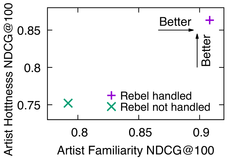
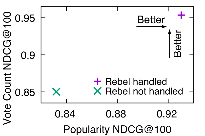
Figure 5. Rebel signals can hurt. MultiImport effectively handles them, achieving a higher accuracy.

Data Fusion and Reconstruction are related to estimating node importance from input signals. Data fusion approaches (Yin et al., 2008; Dong et al., 2009, 2010) integrate potentially conflicting information about entities from multiple data sources (e.g., websites) by considering the trustworthiness of data sources and the dependence between them. Among several values of an object, these methods aim to identify the true value of the object. Our problem setup is related to, but different from data fusion in that our goal is to learn latent node importance which is broadly consistent with input signals, while focusing on a subset of signals which correlate well with each other, instead of identifying which signal value is more accurate than others.

Data reconstruction methods aim to complete missing values in the partially observed data. Matrix and tensor decomposition (Kolda and Bader, 2009; Park et al., 2016, 2017, 2019b; Oh et al., 2019) are representative approaches to this task, which reconstruct observed data using a relatively small number of latent factors. While a rank-1 decomposition of input signals is analogous to our problem, MultiImport simultaneously considers various data sources, such as the KG and input signals, while handling rebel signals and employing GNNs for effective inference over a KG.

Graph Neural Networks apply deep learning ideas to arbitrary graph structured data. These methods have attracted extensive research interest in recent years (Kipf and Welling, 2017; Gilmer et al., 2017; Ying et al., 2018; Xu et al., 2018; Velickovic et al., 2018). Kipf and Welling (Kipf and Welling, 2017) proposed a spectral approach, called GCN, which employs a localized first-order approximation of graph convolutions. More recently, Veličkovič et al. (Velickovic et al., 2018) proposed graph attention networks (GATs) to aggregate localized neighbor information based on attention mechanism. GAT provides an efficient framework to integrate deep learning into graph mining, and has been adopted to recommender systems (Wu et al., 2019), knowledge graph reasoning (Zhang et al., 2019), and graph classification (Lee et al., 2018). While our work is also based on a graph attention architecture, we additionally consider predicates in attention computation, and extend this architecture in a multi-task setting for learning node importance in a KG using multiple signals.

7. Conclusion

Estimating node importance in a KG is a crucial task that has received a lot of interest. A major challenge in successfully achieving this goal is in utilizing multiple types of input effectively. In particular, input signals provide strong evidence for the popularity of entities in a KG. In this paper, we develop an end-to-end framework MultiImport that draws on information from both the KG and external signals, while dealing with challenges arising from the simultaneous use of multiple input signals, such as inferring node importance from sparse signals, and potential conflicts among them. We ran experiments on real-world KGs to show that MultiImport successfully handles these challenges, and consistently outperforms existing approaches. For future work, we plan to develop a method for modeling the temporal evolution of node importance in a KG.

Appendix A Appendix

In the appendix, we present experimental settings.

A.1. Experimental Settings

PageRank (PR) and Personalized PageRank (PPR). We used NetworkX 2.3’s pagerank_scipy function to run PR and PPR. We used the default parameter values set by NetworkX, including the damping factor of 0.85 for both algorithms.

HAR. We implemented HAR in Python 3.7. In experiments, we set $\alpha$ and $\beta$ to 0.15 and $\gamma$ to 0. We ran the algorithm for 30 iterations. Normalized input signal values were used as the probability of entities (as in PPR). All relations were assigned an equal probability. Among hub and authority scores HAR computes for each entity, we used the maximum of the two values as HAR’s estimation, and we observed similar results when reporting only one type of scores.

node2vec. We used the reference node2vec implementation to generate node features. For music10k, fb15k, and tmdb5k, we set the number of dimensions to 64, and for imdb, we set it to 128. For other parameters, we used the default values used by the reference implementation.

GENI. We implemented GENI using the Deep Graph Library 0.3.1. We used GENI with two layers, each consisting of four attention heads. For the scoring network, we used a two-layer fully-connected neural network, where the number of hidden neurons in the first hidden layer was 75% of the input feature dimension. We set the dimensions of predicate embedding to 10. GENI was trained using Adam optimizer with $\beta_{1}=0.9$, $\beta_{2}=0.999$, a learning rate of 0.005, and a weight decay of 0.0005. We applied ReLU to estimated node importance, ELU to node centrality, and Leaky ReLU to unnormalized attention coefficients.

MultiImport. We implemented MultiImport using the Deep Graph Library 0.3.1. For a fair comparison with GENI, we used two layers for MultiImport, and each layer contained four attention heads. The output from each attention head was averaged, and fed into the next layer. For $g(\cdot)$, we used a linear transformation with bias, which projects input features to 75% of the input feature dimension. For $g^{\prime}(\cdot)$, we used another linear transformation with bias. We set the dimension of predicate embedding to 10. For training, we used the Adam optimizer with $\beta_{1}=0.9,\beta_{2}=0.999$, and a learning rate of 0.005. We set $\lambda$ to 0.001. We set $\nu$ to 0.0002 on fb15k and imdb, applying the corresponding loss term in Equation 12 to 20% and 5% of randomly sampled edges, respectively; $\nu$ was set 0.0 on music10k and tmdb5k. ELU was applied for node centrality.

Early Stopping. For MultiImport and GENI, we applied early stopping based on the performance on the validation data set (15% of training data) with a patience of 30, and set the maximum number of iterations to 3000. For testing, we used the model that achieved the best validation performance.

Input Signal Preprocessing. We applied log transformation for all signals as their distribution is highly skewed, except for those signals available on music10k as they are normalized scores.

References

- (1)
- Bollacker et al. (2008) Kurt D. Bollacker, Colin Evans, Praveen Paritosh, Tim Sturge, and Jamie Taylor. 2008. Freebase: a collaboratively created graph database for structuring human knowledge. In SIGMOD. 1247–1250.
- Bordes et al. (2013) Antoine Bordes, Nicolas Usunier, Alberto García-Durán, Jason Weston, and Oksana Yakhnenko. 2013. Translating Embeddings for Modeling Multi-relational Data. In NIPS. 2787–2795.
- Cao et al. (2007) Zhe Cao, Tao Qin, Tie-Yan Liu, Ming-Feng Tsai, and Hang Li. 2007. Learning to rank: from pairwise approach to listwise approach. In ICML. 129–136.
- Dong et al. (2010) Xin Dong, Laure Berti-Équille, Yifan Hu, and Divesh Srivastava. 2010. Global Detection of Complex Copying Relationships Between Sources. Proc. VLDB Endow. 3, 1 (2010), 1358–1369.
- Dong et al. (2009) Xin Luna Dong, Laure Berti-Équille, and Divesh Srivastava. 2009. Integrating Conflicting Data: The Role of Source Dependence. Proc. VLDB Endow. 2, 1 (2009).
- Ester et al. (1996) Martin Ester, Hans-Peter Kriegel, Jörg Sander, and Xiaowei Xu. 1996. A Density-Based Algorithm for Discovering Clusters in Large Spatial Databases with Noise. In KDD. 226–231.
- Gilmer et al. (2017) Justin Gilmer, Samuel S. Schoenholz, Patrick F. Riley, Oriol Vinyals, and George E. Dahl. 2017. Neural Message Passing for Quantum Chemistry. In ICML. 1263–1272.
- Haveliwala (2002) Taher H. Haveliwala. 2002. Topic-sensitive PageRank. In WWW. 517–526.
- Jung et al. (2017) Jinhong Jung, Namyong Park, Lee Sael, and U. Kang. 2017. BePI: Fast and Memory-Efficient Method for Billion-Scale Random Walk with Restart. In SIGMOD.
- Kipf and Welling (2017) Thomas N. Kipf and Max Welling. 2017. Semi-Supervised Classification with Graph Convolutional Networks. In ICLR.
- Kleinberg (1999) Jon M. Kleinberg. 1999. Authoritative Sources in a Hyperlinked Environment. J. ACM 46, 5 (1999), 604–632.
- Kolda and Bader (2009) Tamara G. Kolda and Brett W. Bader. 2009. Tensor Decompositions and Applications. SIAM Rev. 51, 3 (2009), 455–500.
- Lee et al. (2018) John Boaz Lee, Ryan A. Rossi, and Xiangnan Kong. 2018. Graph Classification using Structural Attention. In KDD. 1666–1674.
- Lehmann et al. (2015) Jens Lehmann, Robert Isele, Max Jakob, Anja Jentzsch, Dimitris Kontokostas, Pablo N. Mendes, Sebastian Hellmann, Mohamed Morsey, Patrick van Kleef, Sören Auer, and Christian Bizer. 2015. DBpedia - A large-scale, multilingual knowledge base extracted from Wikipedia. Semantic Web 6, 2 (2015), 167–195.
- Li et al. (2012) Xutao Li, Michael K. Ng, and Yunming Ye. 2012. HAR: Hub, Authority and Relevance Scores in Multi-Relational Data for Query Search. In SDM. 141–152.
- Oh et al. (2019) Sejoon Oh, Namyong Park, Jun-Gi Jang, Lee Sael, and U Kang. 2019. High-Performance Tucker Factorization on Heterogeneous Platforms. IEEE TPDS. 30, 10 (2019), 2237–2248.
- Page et al. (1999) Lawrence Page, Sergey Brin, Rajeev Motwani, and Terry Winograd. 1999. The PageRank citation ranking: Bringing order to the web. Technical Report. Stanford InfoLab.
- Park et al. (2016) Namyong Park, ByungSoo Jeon, Jungwoo Lee, and U Kang. 2016. BIGtensor: Mining Billion-Scale Tensor Made Easy. In CIKM. 2457–2460.
- Park et al. (2019a) Namyong Park, Andrey Kan, Xin Luna Dong, Tong Zhao, and Christos Faloutsos. 2019a. Estimating Node Importance in Knowledge Graphs Using Graph Neural Networks. In KDD. 596–606.
- Park et al. (2017) Namyong Park, Sejoon Oh, and U Kang. 2017. Fast and Scalable Distributed Boolean Tensor Factorization. In ICDE. 1071–1082.
- Park et al. (2019b) Namyong Park, Sejoon Oh, and U Kang. 2019b. Fast and scalable method for distributed Boolean tensor factorization. VLDB J. 28, 4 (2019), 549–574.
- Subramanian et al. (2005) Aravind Subramanian, Pablo Tamayo, Vamsi K Mootha, Sayan Mukherjee, Benjamin L Ebert, Michael A Gillette, Amanda Paulovich, Scott L Pomeroy, Todd R Golub, Eric S Lander, et al. 2005. Gene set enrichment analysis: a knowledge-based approach for interpreting genome-wide expression profiles. Proceedings of the National Academy of Sciences 102, 43 (2005), 15545–15550.
- Tong et al. (2008) Hanghang Tong, Christos Faloutsos, and Jia-Yu Pan. 2008. Random walk with restart: fast solutions and applications. Knowl. Inf. Syst. 14, 3 (2008), 327–346.
- Velickovic et al. (2018) Petar Velickovic, Guillem Cucurull, Arantxa Casanova, Adriana Romero, Pietro Liò, and Yoshua Bengio. 2018. Graph Attention Networks. In ICLR.
- Wang et al. (2017) Quan Wang, Zhendong Mao, Bin Wang, and Li Guo. 2017. Knowledge Graph Embedding: A Survey of Approaches and Applications. IEEE TKDE 29, 12 (2017).
- Wu et al. (2019) Qitian Wu, Hengrui Zhang, Xiaofeng Gao, Peng He, Paul Weng, Han Gao, and Guihai Chen. 2019. Dual Graph Attention Networks for Deep Latent Representation of Multifaceted Social Effects in Recommender Systems. In WWW.
- Xu et al. (2018) Keyulu Xu, Chengtao Li, Yonglong Tian, Tomohiro Sonobe, Ken-ichi Kawarabayashi, and Stefanie Jegelka. 2018. Representation Learning on Graphs with Jumping Knowledge Networks. In ICML. 5449–5458.
- Yin et al. (2008) Xiaoxin Yin, Jiawei Han, and Philip S. Yu. 2008. Truth Discovery with Multiple Conflicting Information Providers on the Web. IEEE TKDE 20, 6 (2008), 796–808.
- Ying et al. (2018) Rex Ying, Ruining He, Kaifeng Chen, Pong Eksombatchai, William L. Hamilton, and Jure Leskovec. 2018. Graph Convolutional Neural Networks for Web-Scale Recommender Systems. In KDD. 974–983.
- Zhang et al. (2019) Wen Zhang, Bibek Paudel, Liang Wang, Jiaoyan Chen, Hai Zhu, Wei Zhang, Abraham Bernstein, and Huajun Chen. 2019. Iteratively Learning Embeddings and Rules for Knowledge Graph Reasoning. In WWW. 2366–2377.