On a Transmission Problem Related to Models of Electrocardiology

Abstract

We a generalization of transmission problems for elliptic matrix operators related to the mathematical models of cardiology. We indicate sufficient conditions providing that the approach elaborated for scalar elliptic operators is still valid in this much more general situation.

Introduction

In this paper we consider a family of transmission problems for elliptic operators with constant coefficients related to models of electrocardiology. More precisely, for many years for satisfactory models of heart activity one uses Cauchy, Dirichlet, and Neumann problems for scalar strongly elliptic operators, see, for example, [1], [2]. A modification of such a model involving boundary problems for the Laplace operator has been recently studied in [3].

We consider similar problems for more general matrix linear elliptic operators and find sufficient conditions under which the scheme for solving the problems suggested in [3] allows to construct their solutions. Our approach is essentially based on the general theory of Fredholm problems for strongly elliptic (matrix) linear operators, see, e.g., [4], and the theory of regularization of an ill-posed Cauchy problem for operators with an injective principal symbol, see [3].

1 A model example

To begin with, we consider a basic example related to models of electrocardiology. As known from clinical practice, see, e.g., [1], [2], electrical activity of cardiac cells is crucial for pumping function of heart, which is the result of rhythmical cycles of contraction-relaxation of the cardiac tissue. Anomalies of electrical activity often cause heart diseases, which makes these investigations, in particular, development of adequate mathematical models, very relevant nowadays.

Let us illustrate this by one model of electrocardiology [1, 2, 5]. Denote by $\Omega_{B}$ and $\Omega_{H}$ three-dimensional domains with piecewise smooth boundaries with $\partial\Omega_{B}$ and $\partial\Omega_{H}$ corresponding to a body and a heart (see Fig. 1). Then the domain $\Omega=\Omega_{B}\setminus\Omega_{H}$ with the boundary $\partial\Omega=\partial\Omega_{B}\cup\partial\Omega_{H}$ corresponds to the body without heart.

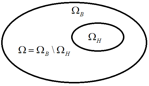
Figure 1: Geometry of the model

Usually, in standard models one assumes that the cardiac tissue can be divided into two parts – intracellular and extracellular parts separated by a membrane – to which the electric potential $u_{i}$ and $u_{e}$, respectively, is assigned. Regarding the cardiac tissue as a continuous medium we think of the potentials as defined in each point of $\Omega_{H}$ and satisfying the equation

$$\nabla^{*}M_{i}\nabla u_{i}+\nabla^{*}M_{e}\nabla u_{e}=0,$$ (1)

where $M_{i}$ and $M_{e}$ are known tensor matrices that characterize intracellular and extracellular parts, and $\nabla$ is the gradient operator in $\mathbb{R}^{3}$.

One often considers the case when $M_{i}$ and $M_{e}$ are positively defined matrices with constant coefficients with entry values defined by conductivity of the cardiac tissue. For simplicity of the further analysis one assumes that these matrices are proportional

$$M_{i}=\lambda M_{e},\quad\ \lambda>0.$$

Based on equation (1) one considers two models of heart activity. In one model it is assumed that the heart is isolated and one considers the problem

$$\begin{gathered}\nabla^{*}M_{i}\nabla u_{i}+\nabla^{*}M_{e}\nabla u_{e}=0\text{ в $\Omega_{H}$},\\ (\nu_{1},\nu_{2},\nu_{3})M_{i}\nabla u_{i}=0\text{ на $\partial\Omega_{H}$},\\ (\nu_{1},\nu_{2},\nu_{3})M_{e}\nabla u_{e}=-(\nu_{1},\nu_{2},\nu_{3})M_{b}\nabla u_{b}\text{ на $\partial\Omega_{H}$},\\ u_{b}=u_{e}\text{ на $\partial\Omega_{H}$},\end{gathered}$$ (2)

where $M_{b}$ is the tensor matrix characterizing conductivity of the body, $\nu$ is the vector field of unit outward normal vectors to the boundary of the domain under the consideration and $u_{b}$ is the electric potential of the body.

In the second model one takes the body into account, and from the electrodynamics of stationary currents it follows that the electric potential of the body $u_{b}$ in the domain $\Omega$ is defined by the equations

$$\begin{gathered}\nabla^{*}M_{b}\nabla u_{b}=0\text{ in $\Omega$},\\ (\nu_{1},\nu_{2},\nu_{3})M_{b}\nabla u_{b}=0\text{ on $\partial\Omega_{B}$}.\end{gathered}$$ (3)

A feature of the model is the fact that one is more interested not in potentials $u_{i}$ and $u_{e}$ separately but in their difference $v=u_{i}-u_{e}$ in $\Omega_{H}$ or at least on its boundary.

Since matrices $M_{i}$ and $M_{e}$ are positively defined and not degenerate, the problems (2), (3) can be studied in the framework of the theory of boundary (maybe ill-posed) problems for elliptic formally self-adjoint equations, see [1, 2, 5]. Moreover, notice that the problems above may be regarded as transmission problems for elliptic equations with discontinuous coefficients describing solutions in different domains of a continuum with the help of additional conditions on separating surfaces, see, for example, [6], [7].

Until now we have not used any functional spaces in the problems description, in the next section we give a precise formulation of a more general problem and specify functional classes for its solution.

2 Formulation of a problem

Let $\theta$ be a measurable set in ${\mathbb{R}}^{n}$, $n\geq 2$. Denote by $L^{2}(\theta)$ a Lebesgue space of complex-valued functions on $\theta$ with the scalar product

$$\left(u,v\right)_{L^{2}(\theta)}=\int_{\theta}\overline{v}(x)u(x)\ dx.$$

If $D$ is a domain in ${\mathbb{R}}^{n}$ with a piecewise smooth boundary $\partial D$, then for $s\in\mathbb{N}$ we denote by $H^{s}(D)$ the standard Sobolev space with the scalar product

$$\left(u,v\right)_{H^{s}(D)}=\int_{D}\sum_{|\alpha|\leq s}\overline{(\partial^{\alpha}v)}(\partial^{\alpha}u)dx.$$

It is well-known that this scale extends for all $s>0$. Let now $H^{s}(D)$ for $s\in{\mathbb{R}}_{+}\setminus{\mathbb{Z}}_{+}$ be the standard Sobolev-Slobodeckij spaces. Denote by $H^{s}_{0}(D)$ the closure of the subspace $C^{\infty}_{\mathrm{comp}}(D)$ in $H^{s}(D)$, where $C^{\infty}_{\mathrm{comp}}(D)$ is the linear space of functions with compact supports in $D$.

The space of $k$-vectors $u=(u_{1},...,u_{k})$ whose components lie in $H^{s}(D)$ equipped with the scalar product

$$\left(u,v\right)_{[H^{s}(D)]^{k}}=\sum_{j=1}^{k}\int_{D}\sum_{|\alpha|\leq s}\overline{(\partial^{\alpha}v_{j})}(\partial^{\alpha}u_{j})dx=\int_{D}\sum_{|\alpha|\leq s}(\partial^{\alpha}v)^{*}(\partial^{\alpha}u)dx$$

we shall denote by $[H^{s}(D)]^{k}$.

Further on, we shall consider linear matrix operators

$$A=\sum_{|\alpha|\leq p}A_{\alpha}\partial^{\alpha},\,x\in D,$$

where $p\in\mathbb{N}$ is the order of operator $A$, $\alpha\in{\mathbb{Z}}^{n}_{+}$, and $A_{\alpha}$ are $(l\times k)$-matrices with constant coefficients. By a formal adjoint of $A$ we call the differential operator

$$A^{*}=\sum_{|\alpha|\leq p}A^{*}_{\alpha}\partial^{\alpha},$$

where $A^{*}_{\alpha}$ is the adjoint matrix for $A_{\alpha}$ or, equivalently,

$$\left(Au,v\right)_{[L^{2}(D)]^{l}}=\left(u,A^{*}v\right)_{[L^{2}(D)]^{k}}\,\ \text{для всех }u\in{\left[C_{0}^{\infty}(D)\right]}^{k},v\in{\left[C_{0}^{\infty}(D)\right]}^{l}.$$

As usual, the principal symbol of an operator $A$ is the matrix

$$\sigma(A)(x,\zeta)=\sum_{|\alpha|=p}A_{\alpha}\zeta^{\alpha},\,x\in D,\,\zeta\in{\mathbb{C}}^{n}.$$

We say that the principal symbol of $A$ is injective if $l\geq k$ and

$$\text{rang}\,\sigma(A)(x,\zeta)=k,\,\ \text{для всех }\zeta\in\mathbb{R}^{n}\setminus\left\{0\right\}\,\ \text{ и всех }x\in\overline{D}.$$

If $l=k$ operators with injective principal symbols are called elliptic.

Let now $A_{e}$, $A_{i}$, and $A_{b}$ be linear differential operators of the first order with constant coefficients on $\overline{D}_{m}$, i.e.

$$A_{m}=\sum_{j=1}^{n}a_{j}^{(m)}\frac{\partial}{\partial x_{j}}+a_{0}^{(m)},\\$$

where $m\in\{e,i,b\}$, $D_{e}\equiv D_{i}\equiv\Omega_{H}$, $D_{b}\equiv\Omega$.

Further on, we assume that principal symbols of operators $A_{m}$ are injective in the corresponding domains.

Denote by $A_{m}^{*}$ a formal adjoint of $A_{m}$ and consider a generalized Laplacian $A_{m}^{*}A_{m}$.

Under assumptions made above, the operator $A_{m}^{*}A_{m}$ is a strongly elliptic $(k\times k)$-matrix second order operator, i.e. it is elliptic and there exists a positive constant $c$ such that

$$\Re\Big{(}-w^{*}\sigma(A_{m}^{*}A_{m})(x,\zeta)w\Big{)}\geq c\left|w\right|^{2}|\zeta|^{2}\,\text{for all }\zeta\in\mathbb{R}^{n}\setminus\left\{0\right\},\,w\in\mathbb{C}^{k}\setminus\left\{0\right\}\,,x\in\overline{D}_{m}.$$

The operator $A_{m}^{*}A_{m}$ is also formally self-adjoint, i.e.

$$\left(A_{m}^{*}A_{m}u,v\right)_{[L^{2}(D_{m})]^{k}}=\left(u,A_{m}^{*}A_{m}v\right)_{[L^{2}(D_{m})]^{k}}=\left(A_{m}u,A_{m}v\right)_{[L^{2}(D_{m})]^{l}}\,\ \text{for all }u,v\in{\left[C_{0}^{\infty}(D_{m})\right]}^{k};$$

in particular, the operator $A_{m}^{*}A_{m}$ is (formally) positively defined

$$\left(A_{m}^{*}A_{m}u,u\right)_{[L^{2}(D_{m})]^{k}}\geq 0\,\ \text{for all }u\in{\left[C_{0}^{\infty}(D_{m})\right]}^{k}.$$

Let, as before, $\nu$ be the outward normal vector operator on the boundary of the domain of the operator $A_{m}$. Introduce the conormal derivatives

$$\nu_{A_{m}}=\sigma^{*}(A_{m})(\nu)A_{m},$$

associated with these operators via Green’s formula:

$$\int_{\partial\Omega}v\nu_{A_{m}}uds=\int_{\Omega}(v^{*}(A_{m}^{*}A_{m}u)-(A_{m}v)^{*}A_{m}u)dx\text{ for all }u,v\in{\left[H^{2}(\overline{D_{m}})\right]}^{k}.$$ (4)

Assume that bounded domains $\Omega_{H}$, $\Omega$, and $\Omega_{b}$ have twice smooth boundaries and consider the following problem (5)-(6): find vector-functions $u_{i}$, $u_{e}$ from ${\left[H^{2}(\Omega_{H})\right]}^{k}$ and a vector-function $u_{b}$ from ${\left[H^{2}(\Omega)\right]}^{k}$ such that

$$\left\{\begin{gathered}A_{i}^{*}A_{i}u_{i}+A_{e}^{*}A_{e}u_{e}=0\text{ in $\Omega_{H}$},\\ \nu_{A_{i}}u_{i}=0\text{ on $\partial\Omega_{H}$},\\ \nu_{A_{e}}u_{e}=-\nu_{A_{b}}u_{b}\text{ на $\partial\Omega_{H}$},\\ u_{e}=u_{b}\text{ на $\partial\Omega_{H}$},\end{gathered}\right.$$ (5)

$$\left\{\begin{gathered}A_{b}^{*}A_{b}u_{b}=0\text{ in $\Omega$},\\ \nu_{A_{b}}u_{b}=0\text{ on $\partial\Omega_{B}$},\end{gathered}\right.$$ (6)

where the equality on the boundary is in the sense of traces, and the equality in the domains is in the sense of distributions. In this case we can assume that traces of functions and their conormal derivatives are well-defined.

It is obvious that the problem (5-6) is a generalization of the problem (2-3). Note also that it incorporates several classical boundary problems.

Example 2.1.

Consider first the classical case $A_{b}=\nabla$ ($k=1$, $l=n$), then $\nu_{A_{b}}=\frac{\partial}{\partial\nu}$ is a directional derivative along the outward normal vector to $\partial\Omega_{B}$. If we assume that $u_{e}$ is known on $\partial\Omega_{H}$ and equal to a function $v_{0}\in H^{3/2}(\partial\Omega_{H})$, then (5-6) gives the following problem: find a function $u_{b}\in H^{2}(\Omega)$ satisfying

$$\left\{\begin{gathered}-\Delta u_{b}=0\text{ in $\Omega$},\\ \frac{\partial u_{b}}{\partial\nu}=0\text{ on $\partial\Omega_{B}$},\\ u_{b}=v_{0}\text{ on $\partial\Omega_{H}$}.\end{gathered}\right.$$ (7)

This is a classical mixed problem that is often called a Zaremba problem, see, e.g. [8], [4]. This problem can be studied by standard methods in Sobolev and Hölder spaces. It is well-known that this problem has a unique solution in these classes that can be written with the help of the Green function ${\mathcal{Z}}_{\Omega}(x,y)$ having the standard properties

$$u_{b}(x)=\int\limits_{\partial\Omega}{\mathcal{Z}}_{\Omega}(x,y)v_{0}(y)dS(y),\,\,x\in\Omega_{H},$$

where $dS(y)$ is the volume form on the surface $\partial\Omega$, see [8], [4].

Analogously, if we assume that $A_{e}=\nabla$ ($k=1$, $l=n$), then $\nu_{A_{e}}=\frac{\partial}{\partial\nu}$ is a directional derivative along the outward normal vector to $\partial\Omega_{H}$. If the conormal derivative $\nu_{A_{e}}u_{e}$ is known on $\partial\Omega_{H}$ and equal to a function $v_{1}\in H^{1/2}(\partial\Omega_{H})$, then (5)-(6) gives a special case of a classical Neumann problem for a Laplace operator: find a function $u_{b}\in H^{2}(\Omega)$ satisfying

$$\left\{\begin{gathered}-\Delta u_{b}=0\text{ в $\Omega$},\\ \frac{\partial u_{b}}{\partial\nu}=0\text{ on $\partial\Omega_{B}$},\\ \frac{\partial u_{b}}{\partial\nu}=v_{1}\text{ on $\partial\Omega_{H}$},\end{gathered}\right.$$ (8)

see [4], [9]. It is known that this problem is Fredholm in Sobolev and Hölder spaces, its solution is defined up to an additive constant, and the necessary and sufficient condition for solvability is the following

$$\int\limits_{\partial\Omega_{H}}v_{1}(y)dS(y)=0.$$ (9)

If this condition is satisfied the problem has a unique solution $u_{b}$ in these classes that satisfies, for example,

$$\int\limits_{\partial\Omega_{H}}u_{b}(y)dS(y)=0.$$ (10)

It can be written with the help of an appropriate parametrix ${\mathcal{N}}_{\Omega}(x,y)$ that has the standard properties

$$u_{b}(x)=\int\limits_{\partial\Omega}{\mathcal{N}}_{\Omega}(x,y)v_{0}(y)dS(y),\,\,x\in\Omega_{H},$$

However, the general theory of boundary problems suggests that knowledge of $u_{e}$ or $\nu_{A_{e}}u_{e}$ on $\partial\Omega_{H}$ does not allow to recover the potential $u_{i}$ uniquely from the remaining data and equations without additional conditions (see also Uniqueness Theorem 3.1 for the problem (5)-(6) proved under additional assumptions below).

Besides that, cardiology models are special in the sense that additional conditions necessary for recovering of unknown potentials $u_{i},\,u_{e},\,u_{b}$ in the problem (5)-(6) should preferably be set on the boundary of ‘the body’ $\Omega$, since all measurements must be less traumatic for a patient and not invasive.

3 Application of an ill-posed Cauchy problem

On of the simplest additional conditions mentioned above leads to using of an ill-posed Cauchy problem. More precisely, it implies measuring the potential $u_{b}$ on the boundary of ‘the body’:

$$u_{b}=f\text{ on $\partial\Omega_{B}$},$$ (11)

where $f$ is a given vector-function from ${\left[H^{3/2}(\Omega)\right]}^{k}$.

Unfortunately, as known very well, the problem (6), (11) is nothing else but an ill-posed problem for an elliptic operator $A_{b}^{*}A_{b}$. Let us see what the addition of the property (11) gives in a more general problem than those in cardiology.

Denote by $N(\Omega)$ the set of solutions to the problem (5), (6), (11) under the condition $f=0$. Let $S_{A_{e}}(\Omega_{H})$ be the space of generalized solutions of the equation $A_{e}h=0$ в $\Omega_{H}$. Since the operator $A_{e}$ has an injective symbol and its coefficients are real analytic, the Petrovsky theorem yields that the elements of the space $S_{A_{e}}(\Omega_{H})$ are real analytic vector-functions in $\Omega_{H}$.

Theorem 3.1.

Let bounded domains $\Omega_{H}$, $\Omega$, and $\Omega_{b}$ have twice smooth boundaries and let for some constant $\lambda>0$,

$$A_{i}=\lambda A_{e}.$$ (12)

Then the set $N(\Omega)$ consists of triples $(u_{i},u_{e},u_{b})\subset{\left[H^{2}(\Omega_{H})\right]}^{k}\times{\left[H^{2}(\Omega_{H})\right]}^{k}\times{\left[H^{2}(\Omega)\right]}^{k}$ such that

$$u_{i}=\frac{h-w}{{\lambda}^{2}},\ \ \ u_{e}=w,\ \ \ u_{b}=0,$$ (13)

where $h$ is an arbitrary function from the space $S_{A_{e}}(\Omega_{H})\cap{\left[H^{2}(\Omega_{H})\right]}^{k}$, and $w$ is an arbitrary function from ${\left[H^{2}_{0}(\Omega_{H})\right]}^{k}$.

Proof.

Let a vector $h$ belong to $S_{A_{e}}(\Omega_{H})\cap{\left[H^{2}(\Omega_{H})\right]}^{k}$ and a vector $w$ belong to ${\left[H^{2}_{0}(\Omega_{H})\right]}^{k}$. Then $w$ satisfies the following conditions

$$w=0\text{ на $\partial\Omega_{H}$,}\,\,\nu_{A_{i}}(w)=0\text{ on $\partial\Omega_{H}$,}$$ (14)

and $A_{i}^{*}A_{i}=\lambda^{2}A_{e}^{*}A_{e}$. Therefore the vector functions from (13) give a solution to the problem (5), (6), (11) for $f=0$.

Let $u_{i},u_{e}\in{\left[H^{2}(\Omega_{H})\right]}^{k}$, and $u_{b}\in{\left[H^{2}(\Omega)\right]}^{k}$ is a triple of functions from $N(\Omega)$. Then from (5)-(6) it follows that $u_{b}$ is a solution to the Cauchy problem for the operator $A_{b}^{*}A_{b}$:

$$A_{b}^{*}A_{b}u_{b}=0\text{ in $\Omega$},\nu_{A_{b}}(u_{b})=0\text{ on $\partial\Omega_{B}$},u_{b}=0\text{ on $\partial\Omega_{B}$}.$$

Since the operators $A_{m}$ have injective symbols, we have

$$\mbox{rang}\,(\nu_{A_{m}})(x,\nu(x))=\sigma^{*}(A_{m})(x,\nu(x))\sigma(A_{m})(x,\nu(x))=k$$

for any $m=e,i,b$ and all $x\in\partial\Omega_{H}$ or $\partial\Omega$, respectively. In particular, the systems of boundary operators $\{I,\nu_{A_{e}}\}$, $\{I,\nu_{A_{i}}\}$ are first order Dirichlet systems on $\partial\Omega_{H}$, while the system of boundary operators $\{I,\nu_{A_{b}}\}$ is a first order Dirichlet system on $\partial\Omega$ (see, for example, [3]). Then by the uniqueness theorem for a Cauchy problem for elliptic operators (see, for example, [3, Theorem 10.3.5]), $u_{b}\equiv 0$ in $\Omega$. Now by the trace theorem for Sobolev spaces and by equations from (5) we see that $u_{e}\equiv 0$ нon $\partial\Omega_{H}$ and $\nu_{A_{e}}(u_{e})\equiv 0$ on $\partial\Omega_{H}$. However, since the system of boundary operators $\{I,\nu_{A_{e}}\}$ is a first order Dirichlet system on $\partial\Omega_{H}$, it follows from the theorem on spectral synthesis (see [10]) that $u_{e}\in[H^{2}_{0}(\Omega_{H})]^{k}$.

To complete the proof of the theorem we need the following lemma.

Lemma 3.1.

Let $\Omega_{H}$ be a bounded domain in $\mathbb{R}^{n}$ with a twice smooth boundary and (12). If the functions $u_{e}$, $u_{i}\in{\left[H^{2}(\Omega_{H})\right]}^{k}$ satisfy the equations (5) then they are related in $\Omega_{H}$ by

$$u_{e}+\lambda^{2}u_{i}=h,$$ (15)

where $h$ as a function from the space $S_{A_{e}^{*}A_{e}}(\Omega_{H})\cap{\left[H^{2}(\Omega_{H})\right]}^{k}$.

Moreover, if $u_{b}\equiv 0$ on $\partial\Omega_{H}$, then the functions $u_{e}$, $u_{i}$ are related in $\Omega_{H}$ by 15, where $h$ is a function from the space $S_{A_{e}}(\Omega_{H})\cap{\left[H^{2}(\Omega_{H})\right]}^{k}$.

Proof.

Since $A_{i}=\lambda A_{e}$, the first equation in (5) can be rewritten in the form

$${A_{e}}^{*}A_{e}h=0\text{ in $\Omega_{H}$},$$ (16)

with $h=u_{e}+\lambda^{2}u_{i}$, and clearly $h\in S_{A_{e}^{*}A_{e}}(\Omega_{H})\cap{\left[H^{2}(\Omega_{H})\right]}^{k}$.

If we additionally know that $u_{b}\equiv 0$ on $\partial\Omega_{H}$ then, as noticed above, $u_{b}\equiv 0$ in $\Omega$. Therefore $\nu_{A_{e}}(u_{e})=0$ on $\partial\Omega_{H}$, and $\nu_{A_{i}}(u_{i})=0$ and $\partial\Omega_{H}$, which implies that

$$\nu_{A_{e}}(h)=0\text{ on $\partial\Omega_{H}$}.$$ (17)

From this, by the Green formula (4) we obtain

$$\begin{gathered}0=(A_{e}^{*}A_{e}h,h)_{[L^{2}(\Omega_{H})]^{k}}=\int\limits_{\Omega_{H}}h^{*}(A_{e}^{*}A_{e}h)dx=\\ =\int\limits_{\Omega_{H}}(A_{e}h)^{*}(A_{e}h)dx+\int\limits_{\partial\Omega_{H}}h^{*}\nu_{A_{e}}(h)ds=\left\|A_{e}h\right\|_{[L^{2}(\Omega_{H})]^{l}}^{2}.\end{gathered}$$

Therefore, the vector function $h$ defined by the equality (15) belongs to $S_{A_{e}}(\Omega_{H})\cap{\left[H^{2}(\Omega_{H})\right]}^{k}$. ∎

Thus, the functions $u_{i},u_{e}\in{\left[H^{2}(\Omega_{H})\right]}^{k}$ satisfy (5), and by Lemma 3.1 we get $u_{i}=\frac{h-v}{{\lambda}^{2}}$, where $v\in[H^{2}_{0}(\Omega_{H})]^{k}$ and $h\in S_{A_{e}}(\Omega_{H})\cap{\left[H^{2}(\Omega_{H})\right]}^{k}$. ∎

In particular, it follows from Lemma 3.1 that the zero space of the problem (5) coincides with the space $S_{A_{e}}(\Omega_{H})\cap{\left[H^{2}(\Omega_{H})\right]}^{k}$.

Denote by $\ker A_{e}$ the kernel of a continuous linear operator $A_{e}:\,[H^{2}(\Omega_{H})]^{k}\rightarrow[H^{1}(\Omega_{H})]^{l}$ and consider several examples. In fact, $\ker A_{e}=S_{A_{e}}(\Omega_{H})\cap{\left[H^{2}(\Omega_{H})\right]}^{k}$.

Example 3.1.

Let $A_{e}=\begin{pmatrix}\nabla\\ 1\end{pmatrix}$, ($k=1$, $l=n+1$). Then $A_{e}^{*}=\begin{pmatrix}-\text{div},1\end{pmatrix}$, $\nu_{A_{e}}=\frac{\partial}{\partial\nu}$, $A_{e}^{*}A_{e}=-\Delta+1$, and the problem (16)-(17) becomes a Neumann problem for the Helmholtz operator

$$\left\{\begin{aligned} -\Delta h+h=0\text{ in $\Omega_{H}$},\\ \frac{\partial h}{\partial\nu}=0\text{ on $\partial\Omega_{H}$},\end{aligned}\right.$$ (18)

and the equation $A_{e}h=0$ takes the form

$$\left\{\begin{aligned} \nabla h=0\text{ in $\Omega_{H}$},\\ h=0\text{ in $\Omega_{H}$}.\end{aligned}\right.$$

Consequently, $\text{ker}A_{e}=\{0\}$ and coincides with the space of solutions of the homogeneous problem (18).

Example 3.2.

Let $A_{e}=\nabla$ then $A_{e}^{*}=-\text{div}$. In this case ($k=1$, $l=n$), $A_{e}^{*}=-\text{div}$, $\nu_{A_{e}}=\frac{\partial}{\partial\nu}$, $A_{e}^{*}A_{e}=-\Delta$, and the problem (16)-(17) becomes a Neumann problem for the Laplace operator

$$\left\{\begin{aligned} \Delta h=0\text{ in $\Omega_{H}$},\\ \frac{\partial h}{\partial\nu}=0\text{ on $\partial\Omega_{H}$},\end{aligned}\right.$$ (19)

and the equation $A_{e}h=0$ takes the form

$$\nabla h=0\text{ in $\Omega_{H}$}.$$

Therefore, $\text{ker}A_{e}=\mathbb{R}$ and coincides with the space of solutions of the problem (19).

Example 3.3.

Consider the case where $A_{e}=\overline{\partial}=\partial_{x}-i\partial_{y}$ is the Cauchy- Riemann operator in ${\mathbb{R}^{2}}\cong\mathbb{C}$ where $i$ stands for imaginary unit. Then $A_{e}^{*}=-\partial=-\partial_{x}-i\partial_{y}$, and the kernel of $A_{e}$ is holomorphic functions. The problem (16)-(17) defines then the zero space of a non- coercive $\overline{\partial}$-Neumann problem, see, for example, [11], [12].

It is clear that the operator $A_{e}$ should be chosen in a way that its kernel is at least finite dimensional.

Under assumptions of Theorem 3.1 the rest of the scheme of solving the problem (5), (6), (11) differs little from the standard one, see [5]. Namely, first we introduce a function $h(x)$ such that $h(x)={\lambda}^{2}u_{i}+u_{e}$, where $x\in\Omega_{H}$. From the conditions on the boundaries in (5) and the fact that $\nu_{A_{i}}=\lambda\nu_{A_{e}}$ we get that

$$\nu_{A_{e}}h=-\nu_{A_{b}}u_{b}\text{ on $\partial\Omega_{H}$}.$$

Thus, we can rewrite the original problem (5), (6), (11) in new notation: knowing a vector $f\in[H^{3/2}(\partial\Omega_{H})]^{k}$, find vectors $h\in[H^{2}(\partial\Omega_{H})]^{k}$ and $u_{b}\in[H^{2}(\partial\Omega)]^{k}$ such that

$$\left\{\begin{gathered}A_{e}^{*}A_{e}h=0\text{ in $\Omega_{H}$},\\ \nu_{A_{e}}h=-\nu_{A_{b}}u_{b}\text{ on $\partial\Omega_{H}$},\\ \end{gathered}\right.$$ (20)

$$\left\{\begin{gathered}A_{b}^{*}A_{b}u_{b}=0\text{ in $\Omega$},\\ \nu_{A_{b}}u_{b}=0\text{ on $\partial\Omega_{B}$},\\ u_{b}=f\text{ on $\partial\Omega_{B}$}.\end{gathered}\right.$$ (21)

The original problem splits into two – (20) and (21). The problem (21), as noticed above, is an ill-posed Cauchy problem for an elliptic operator $A_{b}^{*}A_{b}$. It is known that if a solution to this problem exists it is unique. The problem (20) is a Neumann problem for an elliptic operator $A_{e}^{*}A_{e}$. Unfortunately, in general the Neumann problem may also be ill-posed. For it to be Fredholm, the so called Shapiro-Lopatinsky conditions must be placed [13, Chapter 1, §3, condition II for $q=0$], [14] on the pair $(A_{e}^{*}A_{e},\nu_{A_{e}})$. In particular, they guarantee that the space $S_{A_{e}}(\Omega_{H})\cap[H^{2}(\Omega_{H})]^{k}$ is finite dimensional.

More precisely, let us consider the following Neumann problem: for a given vector $h_{0}\in[H^{1/2}(\partial\Omega_{H})]^{k}$ find a vector $h\in[H^{2}(\partial\Omega_{H})]^{k}$ such that

$$\left\{\begin{gathered}A_{e}^{*}A_{e}h=0\text{ in $\Omega_{H}$},\\ \nu_{A_{e}}h=h_{0}\text{ on $\partial\Omega_{H}$},\\ \end{gathered}\right.$$ (22)

and formulate conditions for solvability.

Theorem 3.2.

If for a pair of operators $(A_{e}^{*}A_{e},\nu_{A_{e}})$ the Shapiro-Lopatinsky conditions are fulfilled then the problem (22) is Fredholm. To be precise,

1. the zero space of the problem coincides with the finite-dimensional space $S_{A_{e}}(\Omega_{H})\cap[H^{2}(\Omega_{H})]^{k}$;

2. the problem is solvable if and only if

   $$(h_{0},\varphi)_{[L^{2}(\partial\Omega_{H})]^{k}}=0\mbox{ for all }\varphi\in S_{A_{e}}(\Omega_{H})\cap[H^{2}(\Omega_{H})]^{k};$$ (23)

3. under (23) there exists a unique solution $h_{1}$ of the problem (22) satisfying

   $$(h_{1},\varphi)_{[L^{2}(\partial\Omega_{H})]^{k}}=0\mbox{ for all }\varphi\in S_{A_{e}}(\Omega_{H})\cap[H^{2}(\Omega_{H})]^{k}.$$ (24)

Proof.

See [4]. ∎

Thus, under hypothesis of Theorem 3.2 for solvability of the Neumann problem (20) it is necessary and sufficient that for the vector $h_{0}=-\nu_{A_{b}}u_{b}$ the condition (23) is fulfilled. This can be achieved if we place additional conditions on relations between the operators $A_{e}$ and $A_{b}$. Namely, as we have seen above, it is quite natural to assume that

$$A_{e}=\tilde{\lambda}A_{b}\mbox{ for some constant }\tilde{\lambda}>0.$$ (25)

Denote by $S_{A_{b}}(\Omega)$ the zero space of solutions to the problem (21) in the domain $\Omega$.

Corollary 3.1.

Let for the pair of operators $(A_{e}^{*}A_{e},\nu_{A_{e}})$ the Shapiro-Lopatinsky conditions be fulfilled. Besides that assume that the identity (25) holds and the spaces $S_{A_{e}}(\Omega_{H})\cap[H^{2}(\Omega_{H})]^{k}$ and $S_{A_{b}}(\Omega)\cap[H^{2}(\Omega)]^{k}$ coincide. Then for any vector $u_{b}\in[H^{2}(\Omega)]^{k}$ satisfying (21) there exists a unique vector $h_{1}\in[H^{2}(\Omega_{H})]^{k}$ that satisfies (20) and (24).

Proof.

By Theorem 3.2 for solvability of the problem (20) it is necessary and sufficient that

$$(\nu_{A_{e}}u_{b},\varphi)_{[L^{2}(\partial\Omega_{H})]^{k}}=0\mbox{ for all }\varphi\in S_{A_{e}}(\Omega_{H})\cap[H^{2}(\Omega_{H})]^{k}.$$ (26)

If the vector $u_{b}\in[H^{2}(\Omega)]^{k}$ satisfies (21), then by the Green formula (4) for the operator $A_{b}$

$$-\int\limits_{\partial\Omega_{H}}\nu_{A_{b}}u_{b}\psi ds=\int\limits_{\partial\Omega}\nu_{A_{b}}u_{b}\psi ds=(\psi,A^{*}_{b}A_{b}u)_{[L^{2}(\Omega)]^{k}}-(A_{b}\psi,A_{b}u)_{[L^{2}(\Omega)]^{k}}=0,$$

for any $\psi\in S_{A_{b}}(\Omega_{H})\cap[H^{2}(\Omega_{H})]^{k}$.

On the other hand, the relation (25) guarantees that $(\tilde{\lambda})^{2}\nu_{A_{b}}=-\nu_{A_{e}}$, and therefore

$$(\nu_{A_{e}}u_{b},\varphi)_{[L^{2}(\partial\Omega_{H})]^{k}}=-(\tilde{\lambda})^{2}(\nu_{A_{b}}u_{b},\varphi)_{[L^{2}(\partial\Omega_{H})]^{k}}=-(\tilde{\lambda})^{2}\int\limits_{\partial\Omega_{H}}\nu_{A_{b}}u_{b}\psi ds$$

for any $\varphi\in S_{A_{e}}(\Omega_{H})\cap[H^{2}(\Omega_{H})]^{k}$. Due to the fact that the spaces $S_{A_{e}}(\Omega_{H})\cap[H^{2}(\Omega_{H})]^{k}$ and $S_{A_{b}}(\Omega)\cap[H^{2}(\Omega)]^{k}$ coincide, (26) holds. Then by statement 3 of Theorem 3.2 for any vector $u_{b}$ there exists a unique vector $h_{1}\in[H^{2}(\Omega_{H})]^{k}$ satisfying (20) and (24). ∎

The condition that the spaces $S_{A_{e}}(\Omega_{H})\cap[H^{2}(\Omega_{H})]^{k}$ and $S_{A_{b}}(\Omega)\cap[H^{2}(\Omega)]^{k}$ coincide seems to be rather strong, especially since these are spaces of solutions to different differential equations in different domains. Nevertheless, provided (25) holds, such a coincidence is possible if the operator $A_{e}$ is so much overdetermined that the space of its solutions in any domain is finite dimensional and coincides with the space of solutions in ${\mathbb{R}}^{n}$; the typical examples are the so-called stationary holonomic systems. Let us illustrate this by the following examples.

Example 3.4.

Let $A_{e}=\nabla$ and $A_{b}=\tilde{\lambda}\nabla$ ($k=1$, $l=n$). The function $u=const$ is a solution to the equation $\nabla u=0$ in $\Omega_{H}$ and extends to $\Omega$, where it is a solution to $\tilde{\lambda}\nabla{u}=0$. Thus we get that the spaces $S_{A_{e}}(\Omega_{H})$ and $S_{A_{b}}(\Omega)$ coincide.

Example 3.5.

Let $A_{e}=\begin{pmatrix}\nabla\\ 1\end{pmatrix}$ and $A_{b}=\tilde{\lambda}\begin{pmatrix}\nabla\\ 1\end{pmatrix}$, ($k=1$, $l=n+1$). A solution to $A_{e}u=0$ in $\Omega_{H}$ is $u\equiv{0}$ and it extends to $\Omega$, where it is a solution $A_{b}u=0$. Thus, the spaces $S_{A_{e}}(\Omega_{H})$ and $S_{A_{b}}(\Omega)$ coincide.

Example 3.6.

Consider the following operators $A_{i}$, $A_{e}$ и $A_{b}$:

$$A_{e}=\begin{pmatrix}\partial_{x}&0&0\\ \partial_{y}&0&0\\ 0&\partial_{x}&0\\ 0&\partial_{y}&0\\ -1&0&\partial_{x}\\ 0&-1&\partial_{y}\\ \end{pmatrix},\,\ A_{i}=\lambda\begin{pmatrix}\partial_{x}&0&0\\ \partial_{y}&0&0\\ 0&\partial_{x}&0\\ 0&\partial_{y}&0\\ -1&0&\partial_{x}\\ 0&-1&\partial_{y}\\ \end{pmatrix},\,\ A_{b}=\tilde{\lambda}\begin{pmatrix}\partial_{x}&0&0\\ \partial_{y}&0&0\\ 0&\partial_{x}&0\\ 0&\partial_{y}&0\\ -1&0&\partial_{x}\\ 0&-1&\partial_{y}\\ \end{pmatrix}.$$

These operators have injective principal symbols and are equivalent to second order operators

$$\tilde{A_{e}}=\begin{pmatrix}\partial_{xx}\\ \partial_{yy}\\ \partial_{xy}\end{pmatrix},\,\,\tilde{A_{i}}=\lambda\begin{pmatrix}\partial_{xx}\\ \partial_{yy}\\ \partial_{xy}\end{pmatrix},\,\,\tilde{A_{b}}=\tilde{\lambda}\begin{pmatrix}\partial_{xx}\\ \partial_{yy}\\ \partial_{xy},\end{pmatrix}.$$

Therefore the space of solutions of the system $A_{e}u=0$ in $\Omega_{H}$ coincides with the set of all linear functions $u=c_{1}x+c_{2}y+c_{3}$, and any function of this form extends to $\Omega$, where it is a solution to the equation $A_{b}u=0$. Therefore, the spaces $S_{A_{e}}(\Omega_{H})$ and $S_{A_{b}}(\Omega)$ coincide.

As noticed above, if a solution to the Neumann problem (20) exists, it is ‘unique’ up to an element of the space $S_{A_{e}}(\Omega_{H})\cap[H^{2}(\Omega_{H})]^{k}$ ( additively).

Recall that the aim of solving the original problem (5), (6), (11) is to find the transmembrane potential $v$ on the surface $\partial\Omega_{H}$. Let us write down the algorithm for solving the problem (20), (21):

1. find a function $u_{b}$ and its conormal derivative $\nu_{A_{b}}(u_{b})$ on the surface $\partial\Omega_{H}$ by solving an ill-posed Cauchy problem (21) for an elliptic operator $A_{b}^{*}A_{b}$.

2. compute values of $h(x)$ on the surface $\partial\Omega_{H}$ by solving a Neumann problem (20) for an elliptic operator $A_{e}^{*}A_{e}$ with the data $\nu_{A_{b}}u_{b}$ on $\partial\Omega_{H}$ obtained in Step 1. The possibility of this depends on whether the restrictions on operators $A_{e}$ and $A_{b}$ described above hold.

3. find the transmembrane potential $v$ on the surface $\partial\Omega_{H}$ by using the relation (15) together with $u_{b}$ and $h$ on $\partial\Omega_{H}$, found in Steps 1 and 2, respectively

   $$v=u_{i}-u_{e}=\frac{h-u_{b}}{{\lambda}^{2}}-u_{b}\text{ on $\partial\Omega_{H}$}.$$ (27)

In conclusion we note that solvability conditions for an ill-posed Cauchy problem in Sobolev spaces for a rather wide class of operators with real analytic coefficients are well known, see, for example, [3]. Moreover, in [3], [15] on can find constructive procedures for its regularization, i.e. for construction exact and approximate solutions (the so called Carleman formulas). Regarding areas with models with the geometry corresponding to that in cardiology and operators that are first order matrix factorizations of the Laplace operator, or more generally, of a Lamé-type operator such Carleman formulas were obtained in [17].

The work was supported by the Foundation for the Advancement of Theoretical Physics and Mathematics “BASIS”.

References

[1] M.Burger, K.A.Mardal, B.F.Nielsen,
Stability analysis of the inverse transmembrane potential problem in electrocardiography,
Inverse Problems, 26(2010), 10, 105012
[2] J.Sundnes, G.T.Lines, X.Cai, B.F.Nielsen, K.A.Mardal, A.Tveito,
Computing the Electrical Activity in the Heart, Springer-Verlag, 2006.
[3] N.N.Tarkhanov, The Cauchy Problem for Solutions of Elliptic Equations, Akademie-Verlag,
Berlin, 1995.
[4] S.Simanca, Mixed Elliptic Boundary Value Problems, Comm. in PDE, 12(1987),
123-200.
[5] V.Kalinin, A.Kalinin, W.H.W.Schulze, D.Potyagaylo, A.Shlapunov,
On the correctness of the transmembrane potential based inverse problem
of ECG, Computing in Cardiology, 2017, 1-4.
[6] M.Schechter, A generalization of the transmission problem,
Ann. SNS di Pisa, Cl. Sci., 14(1960), 3, 207-236.
[7] M.Borsuk, Transmission problem for Elliptic second-order Equations in non-smooth domains,
Birkhäuser, Berlin, 2010.
[8] S.Zaremba, Sur un problème mixte relatif à l’équation de Laplace,
Bull. Acad. Sci. Cracovie, 2(1910), 314–344.
[9] V.P.Mikhailov, Partial differential equations, Nauka, Moscow, 1976 (in Russian).
[10] L.I.Hedberg, T.H.Wolff,
Thin sets in nonlinear potential theory,
Ann. Inst. Fourier, 33(1983), 4, 161–187.
[11] G.B.Folland, J.J.Kohn,
The Neumann Problem for the Cauchy-Riemann Complex,
Princeton University Press, 1973.
[12] A.A.Shlapunov, N.N.Tarkhanov,
On completeness of root functions of Sturm-Liouville problems with discontinuous boundary
operators,
J. of Differential Equations, 255(2013), 3305–3337.
[13] M. S. Agranovich, M. I. Vishik,
Elliptic problems with a parameter and parabolic problems of general type,
Rus. Math. Surv., 19(1964), 3, 53–157.
[14] Z.Ya.Shapiro, On general boundary problems for equations of elliptic type, Izv. Akad.
Nauk SSSR Ser. Mat., 17(1953), 6, 539–562.
[15] A.A.Shlapunov, N.N.Tarkhanov, Bases with double orthogonality in the Cauchy problem for
systems with injective symbols, Proceedings LMS, 3(1995), 1, 1–52.
[16] D.Gilbarg, N.Trudinger, Elliptic Partial Differential Equations of Second Order, Springer-
Verlag, Berlin, 1977.
[17] A.A.Shlapunov,
On the Cauchy Problem for some elliptic systems in a shell in ,
Zeitschrift für Angewandte Mathematik und Mechanik, 77(1997), 11, 849–859.