ELF: An Early-Exiting Framework
for Long-Tailed Classification

Abstract

The natural world often follows a long-tailed data distribution where only a few classes account for most of the examples. This long-tail causes classifiers to overfit to the majority class. To mitigate this, prior solutions commonly adopt class rebalancing strategies such as data resampling and loss reshaping. However, by treating each example within a class equally, these methods fail to account for the important notion of example hardness, i.e., within each class some examples are easier to classify than others. To incorporate this notion of hardness into the learning process, we propose the EarLy-exiting Framework (ELF). During training, ELF learns to early-exit easy examples through auxiliary branches attached to a backbone network. This offers a dual benefit—(1) the neural network increasingly focuses on hard examples, since they contribute more to the overall network loss; and (2) it frees up additional model capacity to distinguish difficult examples. Experimental results on two large-scale datasets, ImageNet LT and iNaturalist’18, demonstrate that ELF can improve state-of-the-art accuracy by more than 3%. This comes with the additional benefit of reducing up to 20% of inference time FLOPS. ELF is complementary to prior work and can naturally integrate with a variety of existing methods to tackle the challenge of long-tailed distributions.

1 Introduction

Real data often follows a long-tailed distribution where the majority of examples are from only a few classes. On datasets following this distribution, neural networks often favor the majority class, leading to poor generalization performance on rare classes. This imbalance problem has traditionally been solved by resampling the data (undersampling, oversampling) [1, 2, 3, 4, 5], or reshaping the loss function (loss reweighting, regularization) [6, 7]. However, these existing approaches focus on class size to address the challenge of data imbalance, without taking into account the “hardness” of each example within a class. Intuitively, there might be easy examples in the minority classes that get incorrectly up-weighted, or difficult examples in the majority classes that get erroneously down-weighted. We show that by incorporating this notion of example hardness during training our method can (correctly) increase the loss contribution of hard examples across all classes.

We propose the EarLy-exiting Framework (ELF) (Figure 1) to incorporate this notion of example hardness during training. ELF is premised around the idea of learning to exit “easy” examples earlier in the network and “harder” examples towards the end. To achieve this, ELF attaches auxiliary classifier branches to a backbone network which we refer to as early-exits. At each early-exit, the neural network tries to correctly predict the input with high confidence. If the prediction is incorrect or the confidence is not high enough (typical for difficult inputs), the example incurs a loss and proceeds to the next exit. Our proposed early-exiting during training has several advantages:

1. Shifting model focus towards harder examples by increasing the average loss contribution of difficult examples compared to easier ones.

2. Freeing model capacity to focus on harder examples by exiting easier ones early in the network.

3. Computational savings during inference by reducing the average FLOPS required per image.

4. Enabling on-the-fly model selection for variable compute budget.

The concept of early-exiting has traditionally been used during inference to reduce the number of floating-point operations (FLOPS) and save energy [8, 9]. In contrast, ELF uses early exiting during training to learn the concept of example hardness which helps with the problem of class imbalance.

Contributions. Our contributions are four-fold: (1) we identify the key concept of example hardness to help improve generalization performance under long-tailed data distributions; (2) we propose ELF, a generic framework that complements existing research by incorporating the notion of example hardness during training; (3) we demonstrate that ELF can generate a family of models to enable on-the-fly model selection for variable computate budgets; (4) we perform extensive evaluation on large-scale imbalanced datasets ImageNet LT and iNaturalist’18, improving the state-of-the-art imbalanced classification accuracy by more than 3%, and reducing FLOPS by up to 20%.

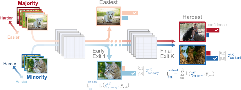
Figure 1: Our EarLy-exiting Framework (ELF) augments a backbone network with auxiliary classifier branches. During training, ELF aims to confidently and correctly classify examples at the earliest possible exit branch. Harder examples exit later in the network, accumulating a higher overall loss.

2 Related Research

Recent research has increasingly shifted focus from classification on artificially balanced datasets [10, 11] to classification under a long-tail class distribution [12, 13]. We discuss closely related research from the areas of long-tailed classification and early-exiting.

Long-tailed classification. Prior work in this area can be categorized along the following three direction—(1) data resampling, (2) loss reshaping, and (3) transfer and meta learning.

Data resampling approaches class imbalance by either repeating examples for the rare class (oversampling) [14, 4, 15, 5] or discarding existing examples from the majority class (undersampling) [14, 16]. The distinguishing factor among these methods lies in the criteria used for under(over)sampling. For example, SMOTE [4] oversamples the minority class through linear interpolation, whereas [16] undersamples by clustering the majority class examples and replacing them with a few anchor points. However, oversampling generally creates redundancy and risks overfitting to rare classes. On the other hand, undersampling is susceptible to losing information from the majority classes [17].

Loss reshaping tackles class imbalance by either reweighting example loss, or through class dependent regularization. Reweighting based approaches assign a larger weight to rare class examples and a smaller weight to the majority ones [6, 18, 19, 20, 21, 22]. On the other hand, regularization methods tackle class imbalance by establishing margins depending upon the class size [23, 24, 25]. Recently, [7] proposed a loss reshaping method (LDAM) to learn larger margins around rare classes. Among loss reshaping methods, the closest to ELF is the Focal loss [26], which incorporates a notion of input-hardness by reweighting an example’s loss in proportion to its prediction confidence. However, in practice Focal loss does not generalize well in the long-tailed setting. ELF complements these existing loss reshaping methods, further improving accuracy under class imbalance.

Transfer and meta learning based approaches aims to transfer knowledge from the majority classes to rare ones by transfer learning, multi task learning or learning to learn [12, 27, 28]. However, it is observed that these approaches are generally more computationally expensive than loss reshaping methods [7], including our proposed method ELF.

Early exiting in neural networks. Research in this area focuses on reducing computation during inference by dynamically routing examples through a network based on their hardness  [8, 29, 30, 31]. The core intuition behind these methods is to reduce the computation during inference by routing easier examples through early exits. Different papers define the notion of hardness differently. For example, [8] defines hardness using the entropy of the prediction vector so that easier examples with low entropy predictions exit earlier. On the other hand [29, 30, 31] defines hardness based on prediction confidence. Thus, (easier) examples with high prediction confidence exit earlier. We note that, these methods focus on early exiting only during inference. In contrast, to the best of our knowledge ELF is the first work that employs early exiting during training to learn the notion of input-hardness. Our extensive experiments suggest this new training approach significantly boosts classification accuracy in the long-tailed setting.

3 ELF: Learning Input-Hardness For Long Tailed Classification

In Section 3.1 we begin by providing some intuition behind ELF; then in Section 3.2 and Section 3.3 we present the technical details of ELF during training and inference, respectively.

3.1 Input-Hardness Intuition

We hypothesize that within both the majority and minority classes some examples are easier than others. Consequently, not every example in the minority class needs to be equally upweighted; and not every example in the majority class needs to be equally downweighted. In order to verify our intuition, we determine what proportion of the rare classes get a high confidence prediction ($\geq 0.9$) and what proportion of the majority classes get a low confidence prediction ($\leq$0.1). Figure 2 plots the prediction confidence versus the proportion of examples (in the class) obtaining that confidence from the CIFAR-10 LT dataset.

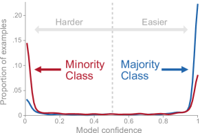
Figure 2: Proportion of examples in class vs. prediction confidence.

As expected, many examples from the minority class are classified with low confidence while many examples from the majority class are predicted with near certainty. However, confirming our hypothesis, a considerable proportion of the minority class examples obtain a high confidence prediction and vice versa. It is precisely this subset of examples—low confidence majority and high confidence minority—that ELF impacts the most. In particular, ELF increases the loss contribution of low confidence majority while retaining the original loss contribution for high confidence minority. This enables a fine-grained, hardness aware approach to loss reweighitng.

Notation. We denote an input example as $\boldsymbol{X}_{i}$ with corresponding label $y_{i}$ that come from a dataset $\mathcal{D}=\{(\boldsymbol{X}_{1},y_{1}),...,(\boldsymbol{X}_{n},y_{n})\}$. The number of training examples in class $j\in\altmathcal{C}$ are denoted by $n_{j}$, and the total number of training examples is $n=\sum_{j=1}^{c}n_{j}$. Without loss of generality, we sort the classes in descending order of cardinality so that $n_{1}\geq...\geq n_{c}$, where $n_{1}\gg n_{c}$ since we operate in the long-tailed setting. Our goal is to learn a neural network $f:\boldsymbol{X}\rightarrow\boldsymbol{z}$ that maps an input space $\boldsymbol{X}$ to a vector of class prediction scores $\boldsymbol{z}=[z_{1},...,z_{c}]^{\top}$, where $z_{i}\in[0,1]\text{ }$. The neural network is parametrized by weights $\boldsymbol{\theta}^{k}$ up to the $k^{th}$ exit. Thus the prediction for input $\boldsymbol{X}_{i}$ at the $k^{th}$ exit is $\boldsymbol{z}_{i}^{(k)}=f(\boldsymbol{X}_{i};\boldsymbol{\theta}^{k})$ where $\boldsymbol{z}_{i}^{(k)}$ is the prediction confidence over $c$ classes. The confidence for the $j^{th}$ class is obtained through indexing as $\boldsymbol{z}_{i}^{(k)}[j]$. Throughout the paper, we use capital bold letters for matrices (e.g., $\boldsymbol{A}$) and lower-case bold letters for vectors (e.g., $\boldsymbol{a}$).

3.2 Early-Exiting During Training

We present the idea of training time early exiting that lies at the core of ELF. As shown in Figure 1, ELF augments a backbone neural network with $K$ auxiliary classifier branches. During training, each input $(\boldsymbol{X}_{i},y_{i})\in\altmathcal{D}$ propagates through all auxiliary exits sequentially until it satisfies the following exit criterion—an example exits only when it is predicted correctly and with a high confidence. More formally, the exit criterion $g^{(k)}_{i}$ for input $\boldsymbol{X}_{i}$ at exit $k$ is

$$g^{(k)}_{i}=\left\{\begin{array}[]{@{}ll@{}}1,&\text{if}\ \operatorname*{argmax}(\boldsymbol{z}_{i}^{(k)})=y_{i}\text{ and }\boldsymbol{z}_{i}^{(k)}[y_{i}]>t^{(k)}\\ 0,&\text{otherwise}\end{array}\right.$$ (1)

Here $t^{(k)}$ is the training time threshold at exit $k$. For simplicity, we chose the same value of $t^{(k)}$ for all exits. By construction, our exit-criterion filters out easy examples early on thereby freeing model capacity for harder examples. Conversely, the harder examples do not satisfy the exit criterion and accumulate additional loss at each exit. Thus, the overall loss contributed by input $\boldsymbol{X}_{i}$ is

$$\mathcal{L}_{\texttt{ELF}}(\boldsymbol{X}_{i},y_{i})=\sum_{k\in[1,...,k^{(e)}_{i}]}\mathcal{L}^{(k)}\left(\boldsymbol{z}^{(k)}_{i},y_{i}\right)\text{ , where }k^{(e)}_{i}=\operatorname*{argmin}_{j\in\{1,2,\ldots,K\}}\left(g_{i}^{(j)}>0\right)$$ (2)

Here $K$ is the total number of exits, and $k^{(e)}_{i}$ denotes the first exit where example $\boldsymbol{X}_{i}$ exits by satisfying the exit criterion in Equation (1). In other words, the ELF framework aggregates loss from each auxiliary branch until the example exits. In contrast, prior work [8, 29] do not perform train time early exiting and aggregates loss from every exit. We believe that by allowing easy examples to exit during training, we can shift the model’s attention to harder examples. by increasing their loss contribution. We believe that this difference—training time early-exiting—is essential for increasing the loss contribution of hard examples.

It is important to note that the ELF loss in Equation (2) is agnostic to the exact instantiation of $\mathcal{L}^{(k)}$ at exit $k$. In paricular, $\mathcal{L}^{(k)}$ can be replaced by any loss function useful for class imbalance, including: weighted cross-entropy [6], Focal [26], LDAM [7] or any combination thereof. In practice, we observe consistent improvements with both weighted cross entropy and the recently proposed LDAM loss. When using class weighted cross-entropy at each exit, ELF loss is described as follows

$$\mathcal{L}_{\texttt{ELF}}^{\texttt{CE}}(\boldsymbol{X}_{i},y_{i})=\sum_{k\in[1,...,k_{i}^{(e)}]}\boldsymbol{w}_{y_{i}}log\left(\frac{exp(\boldsymbol{z}_{i}^{(k)}[y_{i}])}{\sum_{j=1}^{C}exp(\boldsymbol{z}_{i}^{(k)}[j])}\right)$$ (3)

where $\boldsymbol{w}_{y_{i}}$ refers to the class specific weight. Prior work has proposed various strategies to set class weight $\boldsymbol{w}_{y_{i}}$ based on inverse class frequency [22, 19], inverse square root frequency [32, 33] and effective weighting [6]. We leverage the weighting strategy from [6] that sets $\boldsymbol{w}_{c}=\frac{1-\beta}{1-\beta^{n_{c}}}$, where $n_{c}$ is the number of samples in class $c$ and $\beta$ is a hyperparameter with typical values between $\{0.999,0.9999\}$. When using LDAM [7] at each exit, the ELF loss can be described as follows

$$\begin{split}\mathcal{L}_{\texttt{ELF}}^{\texttt{LDAM}}(\boldsymbol{X}_{i},y_{i})&=\sum_{k\in[1,...,k_{i}^{(e)}]}\boldsymbol{w}_{y_{i}}log\left(\frac{exp(\boldsymbol{z}_{i}^{(k)}[y_{i}]-\bigtriangleup_{y_{i}})}{exp(\boldsymbol{z}_{i}^{(k)}[y_{i}]-\bigtriangleup_{y_{i}})+\sum_{j\neq y_{i}}exp(\boldsymbol{z}_{i}^{(k)}[j])}\right)\\ \\ &\text{and }\bigtriangleup_{y_{i}}=\frac{C}{n_{y_{i}}}\end{split}$$ (4)

where $\bigtriangleup_{y_{i}}$ is the per class margin that ensures rare classes get a larger margin. It is determined through a hyperparameter $C$ and the number of examples $n_{y_{i}}$ in class $y_{i}$. We select $C$ such that the largest margin for any class is capped at 0.5 [7].

A desirable outcome of training time early-exiting is that harder examples contribute a higher average loss than easier examples. Formally, we define this through the increasing loss property:

Property 1

(Increasing Loss Property) If $D_{k}$ denotes the set of examples exiting at exit $k$ then $\mathop{\mathbb{E}}_{(\boldsymbol{X}_{i},y_{i})\in D_{1}}[\mathcal{L}_{\texttt{ELF}}(\boldsymbol{X}_{i},y_{i})]<\mathop{\mathbb{E}}_{(\boldsymbol{X}_{i},y_{i})\in D_{2}}[\mathcal{L}_{\texttt{ELF}}(\boldsymbol{X}_{i},y_{i})]<...<\mathop{\mathbb{E}}_{(\boldsymbol{X}_{i},y_{i})\in D_{k}}[\mathcal{L}_{\texttt{ELF}}(\boldsymbol{X}_{i},y_{i})]$.

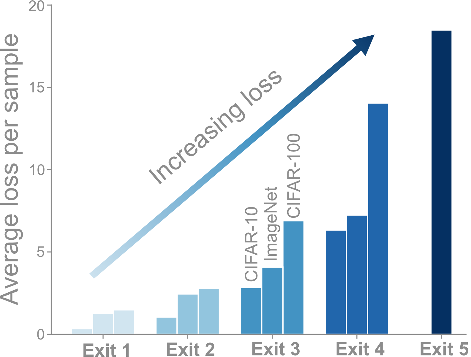
Figure 3: Average per sample loss for images exiting at different exits on three datasets. The increasing trend validates Property 1.

This property enables the neural network to focus on harder examples which contribute a higher expected loss. In Figure 3, we plot the average training loss contributed by examples exiting at different auxillary branches. The increasing trend of average loss across exits validates the increasing loss property.

3.3 Early-Exiting During Inference

Training with ELF loss enables a neural network to learn a notion of input-hardness. During inference, this can be leveraged to early-exit examples from both the minority and majority classes based on hardness. Formally, the inference time early-exit criterion $h^{(k)}_{i}$ (for an input $\boldsymbol{X}_{i}$) at the $k^{th}$ exit is a relaxed version of Equation (1) and defined below:

$$h^{(k)}_{i}=\left\{\begin{array}[]{@{}ll@{}}1,&\text{if}\ \operatorname*{argmax}(\boldsymbol{z}_{i}^{(k)})>s^{(k)}\\ 0,&\text{otherwise}\end{array}\right.$$ (5)

Here $\boldsymbol{z}_{i}^{(k)}$ is the prediction vector for the input $\boldsymbol{X}_{i}$ obtained at exit $k$, and $s^{(k)}$ is the inference time threshold, which for simplicity we set to be the same across all exits. Our inference time exit criterion in Equation (5) exits examples based on prediction confidence which is in line with prior work [9, 34]. Using this criterion, we obtain the prediction vector $\boldsymbol{z}_{i}$ for input $\boldsymbol{X}_{i}$ as

$$\boldsymbol{z}_{i}=\boldsymbol{z}_{i}^{(k^{(e)}_{i})}\text{ , where }k^{(e)}_{i}=\operatorname*{argmin}_{j\in\{1,...,K\}}\left(h_{i}^{(j)}>0\right)$$ (6)

Here $k^{(e)}_{i}$ denotes the first exit where the inference time exit-criterion of Equation (5) holds. We note that the prediction vector $\boldsymbol{z}_{i}$ is determined by both the input $\boldsymbol{X}_{i}$ and the inference exit threshold $s^{(k)}$. Furthermore, reducing $s^{(k)}$ causes more examples to early exit, which in turn leads to a reduction in FLOPS. Thus, given a single model trained using ELF (Equation (2)), varying $s^{(k)}$ offers a way to dynamically generate a family of models with different compute budgets.

4 Experiments

In Section 4.1, we begin by discussing the experimental setup including: (i) evaluated datasets, (ii) model and training configuations, and (iii) loss function setup. Next, in Section 4.2 we extensively analyze ELF’s long-tailed performance and disect its ability to improve upon the state-of-the-art.

4.1 Experimental Setup

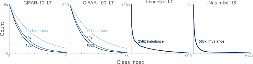
Figure 4: Training distribution for each dataset. On CIFAR-10 and CIFAR-100 we evaluate 3 levels of data imbalance: $10$x, $50$x and $100$x. ImageNet LT and iNaturalist’18 have imbalance ratios of $256\times$ and $500\times$, respectively. For long-tailed datasets, a majority of classes only have a few examples.

Datasets. We conduct our evaluation on four long-tailed datasets: CIFAR-10 LT, CIFAR-100 LT  [6], ImageNet LT [12] and iNaturalist’18 [35]. For the first three datasets, the training split is obtained by subsampling from their balanced versions: CIFAR-10 [36], CIFAR-100 [36] and Imagenet 2012 [37]. In case of the CIFAR LT datasets, we consider three levels of imbalance, $10\times$, $50\times$ and $100\times$, which is defined as the ratio between the number of samples in the largest and the smallest classes. The ImageNet LT training split consists of 115.8k images from 1,000 classes with largest and smallest classes containing 1,280 and 5 images respectively. The iNaturalist’18 dataset is a naturally imbalanced dataset containing 437,513 training images from 8,142 categories with a test set of 24,426 images. Figure 4 highlights the training data distribution for all four datasets. We note that for each dataset, the validation and test sets are balanced across classes and thus top-1 accuracy serves as a common metric of comparison. See the Appendix for additional details on dataset construction.

Backbone models & training configurations. We evaluate several models from the ResNet and DenseNet families. To obtain the ELF models, we attach auxiliary classifier branches before each residual/dense block (see Appendix for details). On CIFAR datasets, we train all ResNet-32 models for 200 epochs using SGD with an initial learning rate of $0.1$ decreased by $0.01$ at epochs $160$ and $180$ [7, 6]. The weight decay is $2\times 10^{-4}$. On ImageNet LT and iNaturalist’18 we train all ResNet-50 and DenseNet-169 models for 100 epochs using SGD with an initial learning rate of 0.1 decreased by 0.1 at epochs 60 and 80. The weight decay is $2\times 10^{-4}$. All models use a linear warmup schedule for the first 5 epochs to avoid initial overfitting in the imbalanced setting [6, 7].

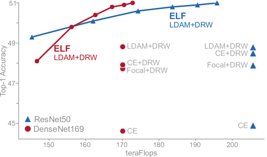
Figure 5: By varying the inference threshold $s^{(k)}$, ELF enables on-the-fly model selection based on the available compute budget (red, blue curves). Each point depicts a ResNet-50 or DenseNet-169 model trained on ImageNet LT for 100 epochs. Observe that the models generated through ELF achieve more than $3\%$ accuracy gains over any other method while using similar or fewer FLOPS.

Implementation. ELF is constructed from three key components—(1) a class reweighting strategy, (2) an exit loss function and (3) a reweighting schedule. For class reweighting, we weight each example of class $c$ according to it’s effective number $\frac{1-\beta}{1-\beta^{n_{c}}}$, where $n_{c}$ is the number of images in class $c$ [6]. For the exit loss, we consider two variations with ELF—at each exit we use either cross entropy loss (CE) or label distribution aware margin loss (LDAM) [7]. These are referred to as ELF(CE) and ELF(LDAM). Finally, for the reweighting schedule we use the per-dataset delayed reweighting (DRW) scheme introduced in [7]. All experiments are conducted in PyTorch 1.0 using an Nvidia DGX-1 containing eight V100 GPUs and 512GB of RAM.

For ELF, we set the training and exit thresholds $t^{(k)},s^{(k)}$ based on the exit loss type. ELF(CE) uniformly sets $t^{(k)}$ = $0.9$ for all exits, while ELF(LDAM) sets $t^{(k)}$ = $2/|c|$, where $|c|$ is the number of classes in the dataset. The inference exit threshold $s^{(k)}$ is identified through a line search. On large datasets, we observe that ELF(LDAM) takes more epochs to converge, therefore we provide results for both 100 and 200 epochs. To measure the performance of ELF, we compare against three strong baselines: CE [6], Focal [26] and LDAM [7], each reusing the same class reweighting and delayed reweighting schedule discussed above. For Focal loss we set $\gamma$ = $0.5$ [26], and for LDAM we set $C$ such that the maximum margin is 0.5 [7]. See Appendix for additional implementation details.

4.2 Evalution on Long-Tailed Classification.

We begin by highlighting ELF’s ability to train once and generate a family of models. Next, we discuss and analyze the performance of ELF on the task of long-tailed classification.

Generating a family of models along the Accuracy-FLOP curve. In Figure 5 we observe the Accuracy-FLOP trade-off for ELF models trained on ImageNet LT. For ELF, the models lie along a curve that offers a favorable accuracy-efficiency tradeoff. The models on this curve are obtained by training once using a fixed training threshold $t^{(k)}$ while linearly varying the inference threshold $s^{(k)}$. This leads to a family of ELF models that enables on-the-fly model selection based on a compute budget. We note that models trained without ELF stack vertically since they consume the same number of inference FLOPS.

Evaluating classification accuracy. In Table 1 All column, we compare the top-1 accuracy of ELF to each baseline configuration on ImageNet LT and iNaturalist’18 datasets. Table 2 presents similar analysis on CIFAR-10/100 LT. In both tables we observe that ELF consistently improves the state-of-the-art accuracy. Moreover the margin of improvement is higher for increasing levels of imbalance (see Table 2). One interesting insight is that ELF improves performance independant of loss type at each exit. Specifically, we see consistent improvements while going from CE [6] to ELF(CE) and from LDAM [7] to ELF(LDAM).

	Imagenet-LT				iNaturalist ’18
	Many	Med	Few	All	Many	Med	Few	All
CE	63.8	38.5	13.6	44.6 (0%)	72.7	63.8	58.7	62.7 (0%)
BBN† [1]	-	-	-	-	-	-	-	69.6 (+100%)
CRT† [2]	58.8	44.0	26.1	47.3 (0%)	69.0	66.0	63.2	65.2 (0%)
LWS† [2]	57.1	45.2	29.3	47.7 (0%)	65.0	66.3	65.5	65.9 (0%)
$\tau$-norm† [2]	56.6	44.2	27.4	46.7 (0%)	65.6	65.3	65.9	65.6 (0%)
CE+DRW [6]	60.3	45.2	27.0	48.5 (0%)	67.1	66.4	65.6	66.1 (0%)
Focal+DRW [26]	59.5	44.6	27.0	47.9 (0%)	66.1	66.0	64.3	65.4 (0%)
LDAM+DRW [7]	61.1	44.7	28.0	48.8 (0%)	70.0	67.4	66.1	67.1 (0%)
ELF(CE) + DRW (100 epochs)	60.7	45.5	27.7	48.9 (-20.7%)	67.4	66.3	65.1	66.0 (-13.5%)
ELF(LDAM) + DRW (100 epochs)	64.0	46.8	27.7	50.8 (-7.4%)	72.3	68.8	65.6	67.9 (-9.0%)
ELF(LDAM)+ DRW (200 epochs)	64.3	47.9	31.4	52.0 (-10.0%)	72.7	70.4	68.3	69.8 (-12.6%)

Table 1: Top-1 accuracy for ResNet-50 trained on Imagenet LT and iNaturalist’18 datasets. The overall accuracy (All column) is decomposed into three splits corresponding to many, medium and few shot settings. Numbers in parenthesis indicate the FLOPS expended by each method relative to the baseline model CE (i.e., more negative means more savings, thus better). ELF consistently improves accuracy while expending fewer FLOPS. ^†Original results from the referenced paper.

	CIFAR-10 Long Tailed			CIFAR-100 Long Tailed
Method	100	50	10	100	50	10
CE	70.4 (0%)	74.8 (0%)	16.4 (0%)	28.3 (0%)	43.9 (0%)	55.7 (0%)
BBN† [1]	79.8 (+100%)	82.2 (+100%)	88.3 (+100%)	42.5 (+100%)	47.0 (+100%)	59.1 (+100%)
Focal† [26]	70.4 (0%)	76.7 (0%)	86.7 (0%)	28.4 (0%)	44.3 (0%)	55.8 (0%)
Mixup† [38]	73.1 (0%)	77.8 (0%)	87.1 (0%)	39.5 (0%)	45.0 (0%)	58.0 (0%)
Manifold Mixup† [39]	73.0 (0%)	78.0 (0%)	87.0 (0%)	38.3 (0%)	43.1 (0%)	56.5(0%)
CE+DRW [6]	76.3 (0%)	80.0 (0%)	87.6 (0%)	41.4 (0%)	46.0 (0%)	58.3 (0%)
Focal+DRW [26]	74.6 (0%)	79.4 (0%)	87.3 (0%)	39.4 (0%)	45.3 (0%)	57.5 (0%)
LDAM+DRW [7]	77.0 (0%)	81.4 (0%)	87.6 (0%)	42.0 (0%)	46.6 (0%)	58.7 (0%)
ELF(CE)+DRW	76.8 (-31.9%)	80.8 (-28.8%)	87.6 (-26.4%)	42.5 (-11.6%)	47.1 (-11.5%)	58.7 (-9.8%)
ELF(LDAM)+DRW	78.1 (-15.1%)	82.4 (-21.4%)	88.0 (-19.6%)	43.1 (-0.01%)	47.5 (-2.39%)	58.9 (-1.9%)

Table 2: Top-1 accuracy for ResNet-32 models trained on long tailed CIFAR-10 and CIFAR-100 datasets. Numbers in parentheses indicate the FLOPS expended relative to the baseline model CE (i.e., more negative means more savings, thus better). Notice that BBN outperforms ELF in some scenarios. This is not surprising since it uses double the number of FLOPS compared to all other methods. ^†These results are referenced from [1].

.

Dissecting the accuracy improvement. To dissect the accuracy of each method, we break down the combined test set into three sets of classes—Many, Medium and Few. These splits refer to classes containing more than 100 examples as Many, classes with 20~100 examples as textitMedium and classes with less than 20 examples as Few [2]. From Table 1 we observe that ELF(LDAM) comprehensively outperforms prior methods on all three splits. Interestingly, we observe that traditional class imbalance techniques sacrifice accuracy on the majority class in order to improve the medium and few classes. In contrast, ELF maintains or improves accuracy across all three class splits.

To ascertain whether the accuracy gains are due to the extra model capacity introduced by exit branches, we calculate the total FLOPS consumed by each model on the test set. The relative FLOPS savings with respect to the baseline model (CE) are presented in parenthesis in Tables 1 and 2. ELF always reduces the FLOPS count, saving up to 20% FLOPS while improving overall accuracy by over 3%. In contrast, a recent method (BBN [1]) achieves similar accuracy by using more than double the FLOPS of the baseline CE model. We ascribe ELF’s improvement in generalization to the hardness aware learning, which we further discuss below.

Visualizing the learned notion of input-hardness. In Figure 6 we present a variety of test set images exiting through auxiliary branches in an ELF ResNet-50 model trained on ImageNet LT. For a particular class, we observe that the object of interest is easier to distinguish in images exiting from earlier branches. For example, consider the lemon class. In the image obtained from exit 1 (column 6, row 3), the object of interest is clearly visible. In comparison, lemon images obtained at exit 3 and (final) exit 5 (column 6, rows 2 and 1), the object of interest is largely obstructed. This highlights that ELF enables a model to learn an intuitive notion of image hardness.

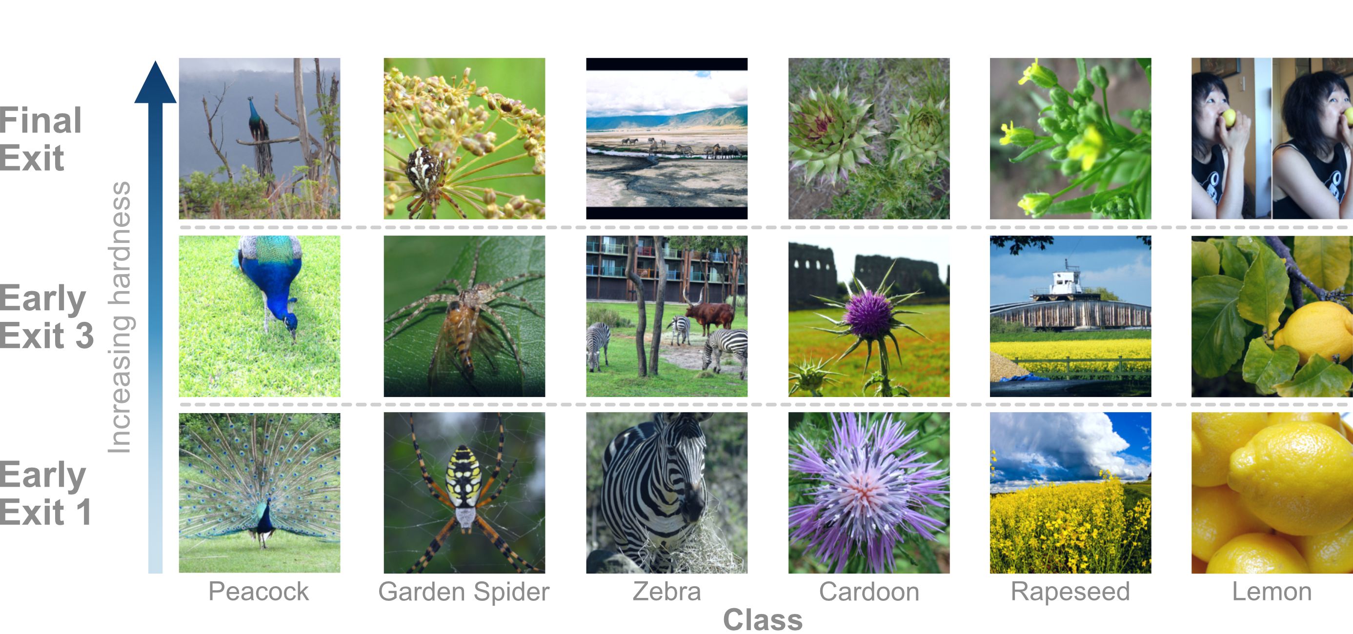
Figure 6: Images exiting from the 1st, 3rd and final exit of the ELF framework. In the 1st exit we observe easy to classify images. As the exits increase, so does the image hardness.

5 Conclusion

We identified the notion of sample-hardness as a key concept to improve generalization under a long-tailed class distribution. To incorporate this notion of hardness in the learning process, we proposed the ELF framework. ELF is complementary to existing work in long-tailed classification and can readily integrate with existing approaches to improve classification accuracy. Extensive evaluations demonstrate that ELF outperforms existing state-of-the-art techniques while enabling on-the-fly model selection for varying compute budgets.

Broader Impact

We describe two scenarios where ELF can have a high impact.

Disease classification. Long-tailed data distributions arise in many real world use cases. For example, a typical prediction task on electric health records (EHR) usually involves classifying over 10,000 diseases codes, many of which are rare. Obtaining good generalization performance on these rare classes is an extremely challenging problem. The largest dataset considered in this paper–iNaturalist’18— contains 8,142 classes and presents a challenge of comparable complexity. On iNaturalist’18, ELF improves state-of-the-art accuracy by over 2.7% (compared to LDAM loss [7]) while saving over $12.5\%$ FLOPS during inference.

Edge device deployment. Another benefit of ELF is that it enables a model to dynamically vary it’s compute footprint during inference. A real-world use case arises when a model is deployed to an edge device (e.g., smartphone, tablet, embedded system). As the battery level decreases, an ELF model can reduce its computational footprint in real time.

Potential weaknesses. Like many deep learning methods, accurate model performance is dependent on large quantities of labeled data. Unfortunately, this is not always available in every domain. In addition, our proposed method is ethically neutral meaning we need to pay attention to how it is used in practice.

Appendix

Appendix A Additional Results on DenseNet-169

In Table 3, we present the top-1 accuracy acheived by a DenseNet-169 model trained on ImageNet LT with various loss functions. Similar to our findings with ResNet-50 (see Table 1 in the main paper), we observe that models trained with ELF(LDAM) improve more than $2.5\%$ on top-1 accuracy while consuming fewer FLOPS. Moreover, the accuracy improvement is acheived on the three class splits corresponding to the Many, Med and Few shot settings.

	Imagenet LT				iNaturalist ’18
	Many	Med	Few	All	Many	Med	Few	All
CE	63.5	38.1	14.4	44.6 (0%)	73.9	64.6	58.1	63.0 (0%)
CE+DRW [6]	60.3	44.2	25.8	47.9 (0%)	68.9	67.3	65.6	66.8 (0%)
Focal+DRW [26]	59.8	44.1	26.0	47.7 (0%)	68.3	66.4	63.6	65.5 (0%)
LDAM+DRW [7]	62.2	44.1	27.6	48.8 (0%)	68.7	67.9	66.5	67.5 (0%)
ELF(LDAM) + DRW (100 epochs)	63.8	46.5	29.0	50.8 (-1.7%)	71.5	68.5	66.2	67.9 (-1.4%)
ELF(LDAM)+ DRW (200 epochs)	64.7	48.2	31.0	52.2 (-2.9%)	71.2	70.6	69.0	70.0 (-6.3%)

Table 3: Top-1 accuracy for DenseNet-169 trained on Imagenet LT and iNaturalist’18 datasets. The overall accuracy (All column) is decomposed into three splits corresponding to many, medium and few shot settings. Numbers in parenthesis indicate the FLOPS expended by each method relative to the baseline model CE (i.e., more negative means more savings, thus better). ELF consistently improves accuracy while expending fewer FLOPS.

Appendix B Hyperparameter search

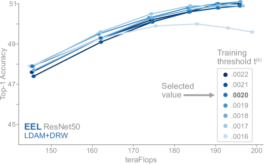
Figure 7: Ablation on training and inference thresholds $t^{(k)},s^{(k)}$. Each point (among a total of 42) represents a Resnet-50 model trained on Imagenet LT using ELF with different values of $(t^{(k)},s^{(k)})$. Each line in the figure connects the points with the same value of $t^{(k)}$ points. The tight clustering of these lines indicates that ELF is robust to the choice of $t^{(k)}$.

We identify the best choice of the training and inference exit thresholds $t^{(k)},s^{(k)}$ through a gridsearch. Figure 7 summarizes the search performed for a ResNet-50 model trained on ImageNet LT dataset using ELF(LDAM). Each point in the figure corresponds to a $(t^{(k)},s^{(k)})$ pair, showing the inference FLOPS (x-axis) and top-1 accuracy (y-axis) achieved by the corresponding model. In total, the Figure 7 plots 42 models corresponding to seven choices of $t^{(k)}\in\{1.6,1.7,1.8,1.9,2,2.1,2.2\}\times 10^{-3}$ and six choices of $s^{(k)}\in\{1.5,1.55,1.6,1.7,1.75\}\times 10^{-3}$. Each line on the plot is obtained by fixing $t^{(k)}$ and varying $s^{(k)}$. The tight clustering of lines reveals that ELF is relatively independent to the choice of the training threshold $t^{(k)}$. This allows us to focus our attention to $s^{(k)}$, which can be used to generate a family of models along an efficiency-tradeoff curve.

Since ELF is robust to $t^{(k)}$ and iterating over it is expensive (evaluating each choice involves training a new model from scratch), in practice, we fix the value of $t^{(k)}$ and iterate only over $s^{(k)}$. Our restricted hyperparameter search for ELF(LDAM) is described as follows. We chose a fixed value of $t^{(k)}=\frac{2}{|c|}$ where $|c|$ is the number of classes in the dataset. For CIFAR-10 LT $|c|=10$, for ImageNet LT $|c|=1000$ and for iNaturalist’18 $|c|=8142$. The inference threshold $s^{(k)}$ is identified by searching across the set $\{1.5,1.55,1.6,1.65,1.7,1.75\}/|c|$. Similarly, for ELF(CE) we select a fixed value of $t^{(k)}=0.9$ for all datasets, and the inference threshold $s^{(k)}$ is searched for across the set $\{0.5,0.55,0.6,0.65,0.7,0.75,0.8,0.85,0.9,0.95\}$.

Appendix C Dataset Construction

The datasets used in this paper are constructed as follows:

CIFAR LT datasets [6]. The training sets for CIFAR-10 LT, CIFAR-100 LT are sampled from the class balanced training sets of CIFAR-10 and CIFAR-100 according to the exponential distribution $n_{c}=n\mu^{c}$. Here $n_{c}$ refers to the remaining number of examples in class $c$, $n$ is the original number of examples per class (5000 for CIFAR-10 and 500 for CIFAR-100) and $\mu\in[0,1]$. We select $\mu$ such that the imbalance ratio—which is defined as the ratio between the number of examples in the largest and smallest class—is $10\times,50\times,100\times$.

ImageNet LT dataset [12]. The training set for the ImageNet LT dataset is sampled from the original training set of ImageNet by following the pareto distribution with the $\alpha=6$. We follow the training split proposed by the original paper [12].

iNaturalist’18 dataset [35]. This is a naturally imbalanced dataset consisting of images from 8,142 species. We use the same training and validation split as the original paper [35].

Appendix D Architecture of ELF models

Recall that ELF augments a backbone model with auxilliary exits. For the ResNet and DenseNet family of models, we attach an auxilliary exit before each residual/dense block. The augmented models are shown in Figure 8, with the auxilliary exit design considerations described below.

ReseNet-32: This backbone model contains three residual block groups (see Figure 8(a)), with each group containing five standard “basic blocks”. Each auxilliary exit consists of two convolution layers with sixty-four kernels of size $3\times 3$, followed by an average pooling and dense layer.

ReseNet-50: This backbone model contains four residual block groups (see Figure 8(b)), with the groups containing $3,4,6$ and $3$ “bottleneck” blocks respectively. Since the filter channels increase rapidly in this architecture (e.g. group three has 1024 channels), we use depthwise separable convolution layers at each exit which helps reduce the additional FLOPS introduced by the auxilliary exits. Each auxilliary exit consists of two convolution layers with $3\times 3$ kernels followed by an average pooling and dense layer. The number of filters in a particular exit is the same as the number of output channels from the preceeding block.

DenseNet-169 This backbone model contains four dense block groups (see Figure 8(c)), with the groups containing $6,12,32$ and $32$ “dense” blocks respectively. Each auxilliary exit consists of two convolution layers with $3\times 3$ kernels followed by an average pooling and dense layer. The number of filters in a particular exit is the same as the number of outuput channels from the preceeding block.

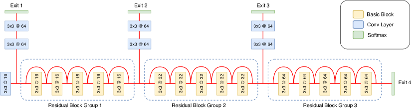
(a) ResNet-32 model with early exits.

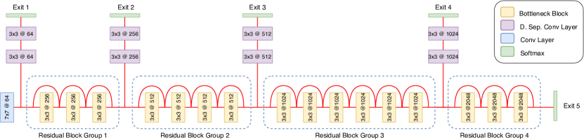
(b) ResNet-50 model with early exits.

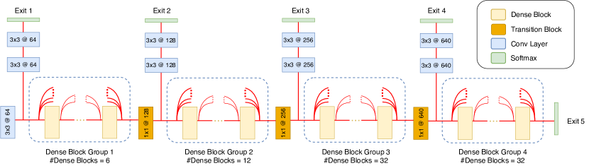
(c) DenseNet-169 model with early exits.

Figure 8: ELF augments a backbone model with auxilliary exits. This figure describes the configuration of the early exits for the three models considered in this work. The notation $3\times 3@16$ indicates that the block / layer contains 16 kernels of size $3\times 3$.

Appendix E Visualizing ELF’s learned notion of hardness

In Figure 9, we provide additional example images exiting from each auxilliary exit of a ResNet-50 model. Similar to our findings in Figure 6 we can see that “harder” images tend to exit from the later exits, indicating that the network trained with ELF(LDAM) indeed learns a notion of example hardness.

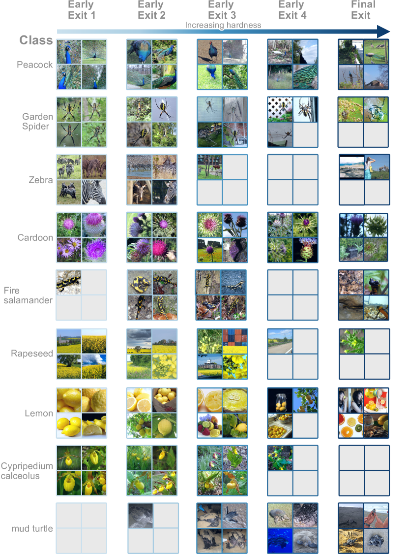
Figure 9: A random sample of images from the ImageNet LT dataset exiting at each auxilliary branch of a ResNet-50 ELF model. As the exits increase, so does the image hardness. Each class containing a gray square indicates no additional images exit from that branch.

References

- [1] Boyan Zhou, Quan Cui, Xiu-Shen Wei, and Zhao-Min Chen. Bbn: Bilateral-branch network with cumulative learning for long-tailed visual recognition. arXiv preprint arXiv:1912.02413, 2019.
- [2] Bingyi Kang, Saining Xie, Marcus Rohrbach, Zhicheng Yan, Albert Gordo, Jiashi Feng, and Yannis Kalantidis. Decoupling representation and classifier for long-tailed recognition. arXiv preprint arXiv:1910.09217, 2019.
- [3] Minlong Peng, Qi Zhang, Xiaoyu Xing, Tao Gui, Xuanjing Huang, Yu-Gang Jiang, Keyu Ding, and Zhigang Chen. Trainable undersampling for class-imbalance learning. In Proceedings of the AAAI Conference on Artificial Intelligence, volume 33, pages 4707–4714, 2019.
- [4] Nitesh V Chawla, Kevin W Bowyer, Lawrence O Hall, and W Philip Kegelmeyer. Smote: synthetic minority over-sampling technique. Journal of artificial intelligence research, 16:321–357, 2002.
- [5] Haibo He, Yang Bai, Edwardo A Garcia, and Shutao Li. Adasyn: Adaptive synthetic sampling approach for imbalanced learning. In 2008 IEEE international joint conference on neural networks (IEEE world congress on computational intelligence), pages 1322–1328. IEEE, 2008.
- [6] Yin Cui, Menglin Jia, Tsung-Yi Lin, Yang Song, and Serge Belongie. Class-balanced loss based on effective number of samples. In Proceedings of the IEEE Conference on Computer Vision and Pattern Recognition, pages 9268–9277, 2019.
- [7] Kaidi Cao, Colin Wei, Adrien Gaidon, Nikos Arechiga, and Tengyu Ma. Learning imbalanced datasets with label-distribution-aware margin loss. In Advances in Neural Information Processing Systems, pages 1565–1576, 2019.
- [8] Surat Teerapittayanon, Bradley McDanel, and Hsiang-Tsung Kung. Branchynet: Fast inference via early exiting from deep neural networks. In 2016 23rd International Conference on Pattern Recognition (ICPR), pages 2464–2469. IEEE, 2016.
- [9] Gao Huang, Danlu Chen, Tianhong Li, Felix Wu, Laurens van der Maaten, and Kilian Q Weinberger. Multi-scale dense networks for resource efficient image classification. arXiv preprint arXiv:1703.09844, 2017.
- [10] Jia Deng, Wei Dong, Richard Socher, Li-Jia Li, Kai Li, and Li Fei-Fei. Imagenet: A large-scale hierarchical image database. In 2009 IEEE conference on computer vision and pattern recognition, pages 248–255. Ieee, 2009.
- [11] Rahul Duggal, Cao Xiao, Richard Vuduc, and Jimeng Sun. Cup: Cluster pruning for compressing deep neural networks. arXiv preprint arXiv:1911.08630, 2019.
- [12] Ziwei Liu, Zhongqi Miao, Xiaohang Zhan, Jiayun Wang, Boqing Gong, and Stella X Yu. Large-scale long-tailed recognition in an open world. In Proceedings of the IEEE Conference on Computer Vision and Pattern Recognition, pages 2537–2546, 2019.
- [13] Rahul Duggal, Scott Freitas, Cao Xiao, Duen Horng Chau, and Jimeng Sun. Rest: Robust and efficient neural networks for sleep monitoring in the wild. In Proceedings of The Web Conference 2020, pages 1704–1714, 2020.
- [14] Dennis L Wilson. Asymptotic properties of nearest neighbor rules using edited data. IEEE Transactions on Systems, Man, and Cybernetics, (3):408–421, 1972.
- [15] Hui Han, Wen-Yuan Wang, and Bing-Huan Mao. Borderline-smote: a new over-sampling method in imbalanced data sets learning. In International conference on intelligent computing, pages 878–887. Springer, 2005.
- [16] Show-Jane Yen and Yue-Shi Lee. Cluster-based under-sampling approaches for imbalanced data distributions. Expert Systems with Applications, 36(3):5718–5727, 2009.
- [17] Mateusz Buda, Atsuto Maki, and Maciej A Mazurowski. A systematic study of the class imbalance problem in convolutional neural networks. Neural Networks, 106:249–259, 2018.
- [18] Chen Huang, Yining Li, Change Loy Chen, and Xiaoou Tang. Deep imbalanced learning for face recognition and attribute prediction. IEEE transactions on pattern analysis and machine intelligence, 2019.
- [19] Yu-Xiong Wang, Deva Ramanan, and Martial Hebert. Learning to model the tail. In Advances in Neural Information Processing Systems, pages 7029–7039, 2017.
- [20] Xiao Zhang, Zhiyuan Fang, Yandong Wen, Zhifeng Li, and Yu Qiao. Range loss for deep face recognition with long-tailed training data. In Proceedings of the IEEE International Conference on Computer Vision, pages 5409–5418, 2017.
- [21] Qi Dong, Shaogang Gong, and Xiatian Zhu. Class rectification hard mining for imbalanced deep learning. In Proceedings of the IEEE International Conference on Computer Vision, pages 1851–1860, 2017.
- [22] Chen Huang, Yining Li, Chen Change Loy, and Xiaoou Tang. Learning deep representation for imbalanced classification. In Proceedings of the IEEE conference on computer vision and pattern recognition, pages 5375–5384, 2016.
- [23] Weiyang Liu, Yandong Wen, Zhiding Yu, and Meng Yang. Large-margin softmax loss for convolutional neural networks. In ICML, volume 2, page 7, 2016.
- [24] Weiyang Liu, Yandong Wen, Zhiding Yu, Ming Li, Bhiksha Raj, and Le Song. Sphereface: Deep hypersphere embedding for face recognition. In Proceedings of the IEEE conference on computer vision and pattern recognition, pages 212–220, 2017.
- [25] Feng Wang, Jian Cheng, Weiyang Liu, and Haijun Liu. Additive margin softmax for face verification. IEEE Signal Processing Letters, 25(7):926–930, 2018.
- [26] Tsung-Yi Lin, Priya Goyal, Ross Girshick, Kaiming He, and Piotr Dollár. Focal loss for dense object detection. In Proceedings of the IEEE international conference on computer vision, pages 2980–2988, 2017.
- [27] Xi Yin, Xiang Yu, Kihyuk Sohn, Xiaoming Liu, and Manmohan Chandraker. Feature transfer learning for face recognition with under-represented data. In Proceedings of the IEEE Conference on Computer Vision and Pattern Recognition, pages 5704–5713, 2019.
- [28] Yin Cui, Yang Song, Chen Sun, Andrew Howard, and Serge Belongie. Large scale fine-grained categorization and domain-specific transfer learning. In Proceedings of the IEEE conference on computer vision and pattern recognition, pages 4109–4118, 2018.
- [29] Gao Huang, Danlu Chen, Tianhong Li, Felix Wu, Laurens van der Maaten, and Kilian Q. Weinberger. Multi-scale dense networks for resource efficient image classification. In ICLR, 2018.
- [30] Mary Phuong and Christoph H Lampert. Distillation-based training for multi-exit architectures. In Proceedings of the IEEE International Conference on Computer Vision, pages 1355–1364, 2019.
- [31] Ting-Kuei Hu, Tianlong Chen, Haotao Wang, and Zhangyang Wang. Triple wins: Boosting accuracy, robustness and efficiency together by enabling input-adaptive inference. arXiv preprint arXiv:2002.10025, 2020.
- [32] Tomas Mikolov, Ilya Sutskever, Kai Chen, Greg S Corrado, and Jeff Dean. Distributed representations of words and phrases and their compositionality. In Advances in neural information processing systems, pages 3111–3119, 2013.
- [33] Dhruv Mahajan, Ross Girshick, Vignesh Ramanathan, Kaiming He, Manohar Paluri, Yixuan Li, Ashwin Bharambe, and Laurens van der Maaten. Exploring the limits of weakly supervised pretraining. In Proceedings of the European Conference on Computer Vision (ECCV), pages 181–196, 2018.
- [34] Mary Phuong and Christoph H. Lampert. Distillation-based training for multi-exit architectures. In The IEEE International Conference on Computer Vision (ICCV), October 2019.
- [35] Grant Van Horn, Oisin Mac Aodha, Yang Song, Yin Cui, Chen Sun, Alex Shepard, Hartwig Adam, Pietro Perona, and Serge Belongie. The inaturalist species classification and detection dataset. In Proceedings of the IEEE conference on computer vision and pattern recognition, pages 8769–8778, 2018.
- [36] Alex Krizhevsky, Geoffrey Hinton, et al. Learning multiple layers of features from tiny images. 2009.
- [37] Olga Russakovsky, Jia Deng, Hao Su, Jonathan Krause, Sanjeev Satheesh, Sean Ma, Zhiheng Huang, Andrej Karpathy, Aditya Khosla, Michael Bernstein, et al. Imagenet large scale visual recognition challenge. International journal of computer vision, 115(3):211–252, 2015.
- [38] Hongyi Zhang, Moustapha Cisse, Yann N Dauphin, and David Lopez-Paz. mixup: Beyond empirical risk minimization. arXiv preprint arXiv:1710.09412, 2017.
- [39] Vikas Verma, Alex Lamb, Christopher Beckham, Amir Najafi, Ioannis Mitliagkas, Aaron Courville, David Lopez-Paz, and Yoshua Bengio. Manifold mixup: Better representations by interpolating hidden states. arXiv preprint arXiv:1806.05236, 2018.