From the Black-Karasinski to the Verhulst model to accommodate the unconventional Fed’s policy.

• In this paper, we argue that some of the most popular short-term interest models have to be revisited and modified to reflect current market conditions better. In particular, we propose a modification of the popular Black-Karasinski model, which is widely used by practitioners for modeling interest rates, credit, and commodities. Our adjustment gives rise to the stochastic Verhulst model, which is well-known in the population dynamics and epidemiology as a logistic model. We demonstrate that the Verhulst model’s dynamics are well suited to the current economic environment and the Fed’s actions. Besides, we derive an integral equations for the zero-coupon bond prices for both the BK and Verhulst (MBK) models. For the BK model for small maturities up to 2 years, we solve the corresponding integral equation by using the reduced differential transform method. For the Verhulst PDE, under some mild assumptions, we find the closed-form solution. Numerical examples show that computationally our approach is more efficient than the standard finite difference method.

Introduction

The Global Economic Crisis (GEC) of 2008-2010 caused unprecedented changes in the way central banks in general, and the mighty Fed in particular, conduct their business. The Quantitative Easing (QE) resulted in central banks embracing the fractional reserve modus operandi. At the same time, commercial banks switched to the narrow bank model, partly by choice and partly by necessity. The Federal Reserve has used short-term interest rates as the policy tool for achieving its macroeconomic goals. As a result, short rates were close to zero for much of the past decade, reflecting the effects of QE, low inflation caused by an aging population, and low productivity growth; see (Rudebusch, 2018). The current economic recession due to the COVID-19 pandemic forces the Fed to push the short interest rates into extremely low or outright negative territory. Given the unprecedented level of unemployment, the economic recession is likely to pave the way for further use of the Fed’s unconventional monetary policy, resulting in meager short rates.

Typically, short-rate interest models use stochastic drivers governed by an Ornstein-Uhlenbeck (OU) process and transform these drivers into the actual rates via suitable mappings. For instance, the Vasicek-Hull-White model uses a linear mapping, while the Black-Karasinski (BK) uses an exponential mapping. The Cox-Ingersoll-Ross model is an exception, which uses a driver governed by a Feller process. For short-rate models driven by OU processes, the rate spends an approximately equal amount of time below and above its equilibrium level. This assumption was valid for decades. However, as was mentioned earlier, it is no longer adequate due to the nontraditional interventions of central banks. Once the rate becomes low, it tends to stay low for a very long time. Under these circumstances, we have to revisit short-rate interest models and modify them to reflect prevailing current market conditions better. With this motivation in mind, we consider the popular BK model, which is widely used by practitioners for modeling interest rates, credit. A similar model, known as the Schwartz one-factor model, is often used to model commodities. The enduring popularity of the model is because, despite some lack of tractability, it is relatively simple and guarantees non-negativity of rates. Besides, one can calibrate it to a given term-structure of interest rates and prices or implied volatilities of caps, floors, or European swaptions, provided that the mean-reversion level and volatility are functions of time.

For the reader’s convenience, we provide some stylized facts about the BK model in Appendix A.1. As can be seen from Eq. (A.1), the short-interest rate $r_{t}$ in this model is lognormal and positive. (If necessary, it can be made negative by using a deterministic shift $s(t)$.) Initially, this positivity was one of the significant advantages of the BK model. However, in the current environment, this feature seems to be less useful. Another problem with the model is in the lognormality of $r_{t}$. Indeed, the lognormality means the CDF of the distribution is right-skewed. Therefore, the time a typical path stays in the lower rate area is short, because the short-rate quickly moves to the mean-reversion level. Accordingly, we need to choose a low mean-reversion speed to rectify this behavior, but the qualitative behavior of $r_{t}$ remains the same. In contrast, given the above discussion, we should design an interest rate model with fat tails at the lower end.

In addition to the structural drawbacks, the BK model is not sufficiently tractable, especially when its coefficients are time-dependent. For instance, prices of zero-coupon bonds (ZCB) and highly liquid barrier options are not known in the closed form. We have to find these prices numerically by solving the corresponding partial differential equations (PDEs), see Eq. (B.1), either via finite differences or asymptotically. In this paper, we present an attractive alternative, by deriving an integral equation for the ZCB price; see Appendix B. The corresponding integral equation can also be solved numerically. Moreover, for small maturities (up to 2 years or so), it can be solved by using the reduced differential transform method; see Appendix C. Numerical examples convincingly show that in this case, our method is more efficient computationally than the standard approach of solving PDEs via finite differences.

In this paper, we propose a modification of the BK model, which organically resolves the lower end fat tail issue, and improves the model tractability. We describe the model in the next Section. We also present an integral equation for the ZCB price for our model and provide a closed-form solution of the model PDE in a particular case. We demonstrate that this solution accelerates the computation of the ZCB prices and provides a basis for efficient calibration.

1 The modified BK (MBK/Verhulst) model

Since the BK model doesn’t support fat tails at the lower end, besides not being analytically tractable, we introduce its modified version of the form

$$dz_{t} =\kappa(t)[\bar{\theta}(t)-e^{z_{t}}]dt+\sigma(t)dW_{t},$$ (1)

$$r_{t} =s(t)+Re^{z_{t}},\qquad R=r_{0}-s(0),\qquad(t,z_{t})\in[0,T]\times(-\infty,\infty).$$

In other words, we modify the dynamics of the stochastic variable $z_{t}$ in Eq. (A.1) in the mean-reversion term by replacing $z_{t}$ with $e^{z_{t}}$.

In Eq. (1) $r_{t}$ is the short interest rate, $t$ is the time, $W_{t}$ is the standard Brownian motion, $\kappa(t)>0$ is the speed of mean-reversion, $\bar{\theta}(t)$ is the mean-reversion level, $\sigma(t)$ is the volatility, $R$ is some constant with the same dimensionality as $r_{t}$, eg., it can be $R=r(0)-s(0)$, T is the maturity. This model is similar to the Hull-White model, but preserves positivity of $r_{t}$ by exponentiating the OU random variable $z_{t}$. Because of that, usually practitioners add a deterministic function (shift) $s(t)$ to the definition of $r_{t}$ to address possible negative rates and be more flexible when calibrating the term-structure of the interest rates.

It can be seen, that at small $t$ $|z_{t}|\ll 1$, and so choosing $\bar{\theta}(t)=1+\theta(t)$ replicates the BK model in the linear approximation on $z_{t}$. Similarly, the choice $\bar{\theta}(t)=e^{\theta(t)}$ replicates the BK model at $z_{t}$ close the mean-reversion level $\theta(t)$. Thus, the modified BK model acquires the properties of the BK model while is a bit more tractable as this will be seen below.

By Itô’s lemma and the Feynman–Kac formula any contingent claim written on the $r_{t}$ as the underlying (for instance, the price $F({\bar{r}},t,T)$ of a Zero-coupon bond (ZCB) with maturity $T$) solves the following partial differential equation

$$0 =\frac{\partial F}{\partial t}+\frac{\displaystyle 1}{\displaystyle 2}\sigma^{2}(t){\bar{r}}^{2}\frac{\partial^{2}F}{\partial{\bar{r}}^{2}}+\kappa(t){\bar{r}}[{\tilde{\theta}}(t)-{\bar{r}}]\frac{\partial F}{\partial{\bar{r}}}-(s(t)+R{\bar{r}})F,$$ (2)

$${\bar{r}}_{t} =\frac{r_{t}-s(t)}{r_{0}-s(0)}=e^{z_{t}},\qquad{\tilde{\theta}}(t)={\bar{\theta}}(t)+\frac{\sigma^{2}(t)}{2\kappa(t)}.$$

This equation should be solved subject to the same terminal and boundary conditions as in Eq. (B.2)

$$F(T,{\bar{r}})=1,\qquad F(t,{\bar{r}})\Big{|}_{{\bar{r}}\to\infty}=0.$$ (3)

Note that since ${\bar{r}}\in(0,\infty)$, i.e., the boundary ${\bar{r}}=0$ is not attainable, Eq. (2) doesn’t need the boundary condition at the left boundary ${\bar{r}}\to 0$, as this is discussed in (Itkin and Muravey, 2020) with a reference to Fichera theory (in other words, the PDE itself with substituted ${\bar{r}}=0$ serves as the boundary condition). If, however, the boundary ${\bar{r}}=0$ is attainable, the boundary condition at this point should be set as in Eq. (29). This is also applicable to all below PDEs obtained from Eq. (2) by transformations.

It is worth noting that Eq. (2) is the stochastic Verhulst or stochastic logistic model, which are well-known in the population dynamics and epidemiology; see, eg., (Verhulst, 1838; Bacaer, 2011; Giet et al., 2015) and references therein. In the past, several authors attempted to use this model in finance; see, eg., (Chen, 2010; Londono and Sandoval, 2015; Halperin and Feldshteyn, 2018). In our case, the stochastic Verhulst equation has the form

$$d{\bar{r}}_{t} =k(t){\bar{r}}_{t}[{\tilde{\theta}}(t)-{\bar{r}}_{t}]dt+\sigma(t){\bar{r}}_{t}dW_{t},$$ (4)

$${\bar{r}}_{t} =[r_{t}-s(t)]/R,\qquad r(t=0)=r_{0}.$$

Eq. (4) can be explicitly solved (for the time-homogeneous coefficients this is done, eg., in (Giet et al., 2015), Proposition 3.3). The following Proposition holds

Proposition 1.

The Eq. (4) admits a unique positive solution ${\bar{r}}_{t}$

$${\bar{r}}_{t}=\frac{1}{\kappa(t)}\frac{X_{t}}{\frac{T_{0}}{\kappa(0){\bar{r}}_{0}}+\int_{0}^{t}X_{q}dq},\qquad t\geq 0,$$ (5)

where $X_{t}$ solves the lognormal SDE

$$dX_{t}=\mu(t)X_{t}dt+\sigma(t)X_{t}dW_{t},\qquad\mu(t)=\frac{\kappa^{\prime}(t)}{\kappa(t)}+\kappa(t){\tilde{\theta}}(t).$$ (6)

Also,

1. The diffusion ${\bar{r}}_{t}$ is recurrent if and only if $q(t)\leq 0$, where $q(t)=\frac{1}{2}-\frac{\kappa(t){\tilde{\theta}}(t)}{\sigma^{2}(t)},\ \forall t\in[0,T]$.

2. If $q(t)<0,\ \forall t\in[0,T]$, assuming that the limits of $q(t)$ and $\sigma^{2}(t)/(2\kappa(t)$ exist at $t\to\infty$, the diffusion ${\bar{r}}_{t}$ converges in law towards the unique stationary Gamma probability distribution $\Gamma\left(-2q(t),\sigma^{2}(t)/(2\kappa(t)\right)_{t\to\infty}$.

3. If $\exists t_{*}\geq 0:q(t_{*})>0$, the diffusion goes a.s. to zero when time goes to infinity.

Proof.

The proof can be obtained by applying Itô’s lemma to Eq. (5) and using Eq. (6). The second part follows from Proposition 3.3 in (Giet et al., 2015). It is interesting to note, that the condition $q<0$ is precisely the Feller condition for the famous CIR model, (Andersen and Piterbarg, 2010). ∎

Thus, the stationary distribution for the Verhulst model is the Gamma distribution. It is easy to check that as compared with the mean-reversion lognormal model (the BK model) with the same parameters, the former has much fatter tails at the lower end, while the latter has the fatter tails when ${\bar{r}}_{t}\to\infty$. However, since, under the current market conditions, we are interested in modeling the lower end in the first place, the Verhulst model has a distinct advantage compared with the BK model. In other words, the probability of having lower rates for the Verhulst model is much higher than for the BK model, and comes naturally.

To illustrate this in a slightly different way, we produce a set of Monte-Carlo paths for both models which have the same volatility and mean-reversion rate, while the mean -reversion level $\bar{\theta}(t)$ in Eq. (1) is chosen as $\bar{\theta}(t)=1+\theta(t)$, so the dynamics Eq. (1) corresponds to the BK dynamics in Eq. (A.1) for small $z_{t}$. The results obtained by using parameters given in Section 4 are presented in Fig. 1, which shows that $r_{BK}$ is always higher than $r_{Vh}$, which confirms our theoretical observation in above.

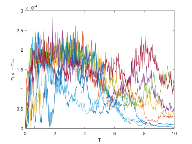
Figure 1: Typical paths of the difference $r_{BK}-r_{Vh}$ for the short-term BK and Verhulst interest rates as a function of time.

Next, we aim to demonstrate that the Verhulst model is also more tractable than the BK model.

2 An integral equation for the ZCB price in the Verhulst model

In this section, we find the value of the ZCB by deriving and solving a Volterra integral equation of the second kind. We proceed with the elimination of the squared term in the drift in Eq. (2) via the following change of variables

$$F(t,{\bar{r}})=e^{\frac{\kappa(t)}{\sigma^{2}(t)}{\bar{r}}+\int_{T}^{t}s(k)dk}W(t,{\bar{r}}).$$ (7)

This yields

$$0=\frac{\partial W}{\partial t} +\frac{\displaystyle 1}{\displaystyle 2}\sigma^{2}(t){\bar{r}}^{2}\frac{\partial^{2}W}{\partial{\bar{r}}^{2}}+\kappa(t){\tilde{\theta}}(t){\bar{r}}\frac{\partial W}{\partial{\bar{r}}}+\left[\gamma(t){\bar{r}}-\frac{\kappa^{2}(t)}{2\sigma^{2}(t)}{\bar{r}}^{2}\right]W,$$

$$\gamma(t) =-R+\frac{\kappa^{2}(t){\tilde{\theta}}(t)}{\sigma^{2}(t)}+\frac{d}{dt}\left(\frac{\kappa(t)}{\sigma^{2}(t)}\right),$$

$$W(T,{\bar{r}}) =e^{-\frac{\kappa(T)}{\sigma^{2}(T)}{\bar{r}}},\qquad W(T,{\bar{r}})\Big{|}_{{\bar{r}}\to\infty}=0.$$ (8)

Another change of variables

$$W(t,{\bar{r}}) =u(\tau,y),\qquad y=\log{\bar{r}}+\int_{0}^{t}\left[\frac{\sigma^{2}(k)}{2}-\kappa(k){\tilde{\theta}}(k)\right]dk,\qquad\tau=\frac{1}{2}\int_{t}^{T}\sigma^{2}(k)dk$$ (9)

transforms this PDE into the following one

$$\frac{\partial u}{\partial\tau} =\frac{\partial^{2}u}{\partial y^{2}}+\left[\alpha(\tau)e^{y}+\beta(\tau)e^{2y}\right]u,$$ (10)

$$\alpha(\tau) =\frac{2\gamma(t(\tau))}{\sigma^{2}(t(\tau))}e^{-\int_{0}^{t}\left[\frac{\sigma^{2}(k)}{2}-\kappa(k){\tilde{\theta}}(k)\right]dk},\qquad\beta(\tau)=-\frac{\kappa^{2}(t(\tau))}{\sigma^{4}(t(\tau))}e^{-\int_{0}^{t}\left[\sigma^{2}(k)-2\kappa(k){\tilde{\theta}}(k)\right]dk}.$$

It is worth mentioning that, by the change of variables $y\to-y$ and $\tau\to-\mathrm{i}\mkern 1.0mu\tau$, this PDE transforms into the time-dependent Schrödinger equation with the unsteady Morse potential.

This PDE in Eq. (10) should be solved subject to the initial and boundary conditions (see discussion in (Itkin and Muravey, 2020))

$$u(0,y) =\exp[-B(T)e^{y-A(T)}],\qquad u(\tau,y)\Big{|}_{y\to\infty}=0,$$ (11)

$$B(T) =\frac{\kappa(T)}{\sigma^{2}(T)},\qquad A(T)=\int_{0}^{T}\left[\frac{\sigma^{2}(k)}{2}-\kappa(k){\tilde{\theta}}(k)\right]dk.$$

Since $u(0,y),\ y\in(-\infty,\infty)$, $u(0,y)$ can be represented as

$$u(0,y)=\frac{1}{2}-\frac{1}{2}(H(y)-H(-y))+g(y),\qquad g(\infty)=g(-\infty)=0,$$

where $H(y)$ is the Heaviside step function. The Fourier transforms of all parts in the RHS of this equation exist implying that it also exists for $u(0,y)$. Therefore, applying the Fourier transform

$${\bar{u}}(\tau,\omega)=\int_{-\infty}^{\infty}u(\tau,y)e^{-i\omega y}dy,$$ (12)

to both parts of Eq. (10) yields the ordinary differential equation

$$\frac{d{\bar{u}}}{d\tau} +\omega^{2}{\bar{u}}=g(\tau,\omega),$$ (13)

$$g(\tau,\omega) =\int_{-\infty}^{\infty}u(\tau,y)\left[\alpha(\tau)e^{y}+\beta(\tau)e^{2y}\right]e^{-i\omega y}dy,\qquad{\bar{u}}(0,\omega)=\int_{-\infty}^{\infty}u(0,y)e^{-i\omega y}dy.$$

The solution of this problem can be written as

$${\bar{u}}(\tau,\omega)=e^{-\omega^{2}\tau}{\bar{u}}(0,\omega)+\int_{0}^{\tau}e^{-\omega^{2}(\tau-s)}g(s,\omega)ds$$ (14)

Now, applying the inversion formula

$$u(\tau,y)=\frac{1}{2\pi}\int_{-\infty}^{\infty}{\bar{u}}(\tau,\omega)e^{i\omega y}d\omega,$$

we obtain the following representation for $u(\tau,y)$

$$u(\tau,y)=\frac{1}{2\pi}\int_{-\infty}^{\infty}\left[e^{-\omega^{2}\tau}{\bar{u}}(0,\omega)+\int_{0}^{\tau}e^{-\omega^{2}(\tau-s)}g(s,\omega)ds\right]e^{i\omega y}d\omega$$ (15)

Substituting the explicit representations for ${\bar{u}}(0,\omega)$ and $g(\tau,\omega)$ into Eq. (15), and taking into account that the function $e^{-\omega^{2}\tau}$ is an even function, we obtain

$$u(\tau,y)=\frac{1}{\pi}\int_{0}^{\infty}\bigg{\{} e^{-\omega^{2}\tau}\int_{-\infty}^{\infty}u(0,\xi)\cos[\omega(y-\xi)]d\xi$$ (16)

$$+\int_{0}^{\tau}ds\,e^{-\omega^{2}(\tau-s)}\int_{-\infty}^{\infty}u(\tau,\xi)\left[\alpha(s)e^{\xi}+\beta(s)e^{2\xi}\right]\cos[\omega(y-\xi)]d\xi\bigg{\}}d\omega.$$

Applying the identity ((Gradshtein and Ryzhik, 2007))

$$\int_{-\infty}^{\infty}e^{-\beta x^{2}}\cos(bx)dx=\sqrt{\frac{\pi}{\beta}}\exp\left(-\frac{b^{2}}{4\beta}\right),$$

and changing the order of integration, we get the integral equation for $u(\tau,y)$

$$u(\tau,y)=\frac{1}{2\sqrt{\pi}}\Bigg{\{}\int_{-\infty}^{\infty}\frac{u(0,\xi)}{\sqrt{\tau}}e^{-\frac{(y-\xi)^{2}}{4\tau}}d\xi+\int_{-\infty}^{\infty}d\xi\int_{0}^{\tau}\frac{u(k,\xi)}{\sqrt{\tau-k}}e^{-\frac{(y-\xi)^{2}}{4(\tau-k)}}\left[\alpha(k)e^{\xi}+\beta(k)e^{2\xi}\right]dk\Bigg{\}}.$$ (17)

This is a two-dimensional Volterra equation of the second kind, see (Lipton, 2001; Lipton and Kaushansky, 2020; Itkin and Muravey, 2020; Carr et al., 2020) for the discussion. As mentioned by an anonymous referee, this equation is also a direct consequence of the Duhamel’s principle.

As far as the numerical solution of Eq. (17) is concerned, the simplest scheme would be Picard iterations. First, we can change the order of integration, so the integral in time becomes the outer one. It can be approximated by using, eg. the trapezoidal rule. Then the coefficients of integration can be computed by using Fast Gauss Transform with the complexity $O(NM)$, $N$ is the number of grid points in $y$, $M$ - in $\tau$. And computing the outer integral requires $O(M^{2})$ operations. Thus, if $M\leq N$ the speed of the method is same as of a FD scheme with the second order of approximation in space and time (eg,, the Crank-Nicolson one). However, using higher order Simpson quadratures can reduce $M$ to $\sqrt{M}$ providing same accuracy, while doing same for the FD method is not trivial. We discuss this in more detail below in the paper.

3 A closed-form solution for the ZCB price in the MBK model

Here, we show that for some dependencies between the parameters of the model, the Cauchy problem Eq. (2) can be solved explicitly in terms of the Gauss hypergeometric function, (Abramowitz and Stegun, 1964).

We start with the following change of variables

$$x=\phi(t){\bar{r}},\qquad\phi(t)=e^{\int_{0}^{t}\left[C_{\alpha}\sigma^{2}(k)-\kappa(k){\tilde{\theta}}(k)\right]dk},$$ (18)

where $C_{\alpha}$ is a constant. This change of variables yields

This change of variables yields

$$0 =\frac{\partial W}{\partial t}+\frac{\displaystyle 1}{\displaystyle 2}\sigma^{2}(t)x^{2}\frac{\partial^{2}W}{\partial x^{2}}+C_{\alpha}\sigma^{2}(t)x\frac{\partial W}{\partial x}+\left[\frac{\gamma(t)}{\phi(t)}x-\frac{\kappa^{2}(t)}{2\sigma^{2}(t)\phi^{2}(t)}x^{2}\right]W$$ (19)

$$W(T,x) =e^{-\frac{\kappa(T)}{\sigma^{2}(T)\phi(T)}x},\qquad W(T,x)\Big{|}_{x\to\infty}=0.$$

We assume $\kappa(t)$, ${\tilde{\theta}}(t)$ and $\sigma(t)$ satisfy the following conditions

$$C_{\gamma}=\frac{\gamma(t)}{\kappa(t)},\qquad C_{\sigma}=\frac{\sigma^{2}(t)\phi(t)}{2\kappa(t)},$$ (20)

where $C_{\gamma}$ and $C_{\sigma}>0$ are some constants. Using the definitions of $\gamma(t),\phi(t)$, and some algebra, we can show that under these conditions, we have

$$C_{\gamma} =C_{\alpha}-\frac{R}{\kappa(t)},\qquad C_{\sigma}=\frac{\sigma^{2}(0)}{2\kappa(t)},\qquad{\tilde{\theta}}(t)=\frac{C_{\alpha}\sigma^{2}(t)}{\kappa(t)}+\frac{2}{\kappa(t)}\frac{\sigma^{\prime}(t)}{\sigma(t)},\qquad\phi(t)=\frac{\sigma^{2}(0)}{\sigma^{2}(t)}.$$ (21)

The first equality implies that in this case the mean reversion rate $\kappa(t)=\kappa=const$, and $C_{\gamma}$ depends on $C_{\alpha}$ and $\kappa$, while $C_{\sigma}$ depends on $\kappa$ and $\sigma(0)$. It means that we can calibrate the model as follows. First, we calibrate the volatility term structure to the market, together with the constant mean reversion rate of $\kappa$ and the constant $C_{\alpha}$. Second, we determine the time-dependent mean-reversion level ${\tilde{\theta}}(t)$ by using Eq. (21). Thus, in this version of the model, we have three calibration parameters: two of them - $\kappa$ and $C_{\alpha}$ are constants, and the normal volatility $\sigma(t)$ is time-dependent. In other words, this enables capturing the volatility term-structure of the market which seems to be the most important property, while assuming a constant mean reversion speed is not too restrictive. The time-dependence of the mean reversion level, however, is fully defined by $\sigma(t)$ and is corrected by another calibrated constant $C_{\alpha}$. So this seems to be a weak side of the model.

Now, applying another change of variables to Eq. (19)

$$w =\frac{x}{C_{\sigma}},\qquad\tau=\frac{1}{2}\int_{t}^{T}\sigma^{2}(k)\,dk,\qquad W(t,x)=w^{-C_{\alpha}}e^{C_{\alpha}(1-C_{\alpha})\tau}u(\tau,w),$$ (22)

we obtain the PDE with the time-homogeneous coefficients

$$0=\frac{\partial^{2}u}{\partial w^{2}}+\left[-\frac{1}{4}+\frac{C_{\gamma}}{w}\right]u-\frac{1}{w^{2}}\frac{\partial u}{\partial\tau}.$$ (23)

This PDE should be solved subject to the initial and boundary conditions

$$u(0,w)=w^{C_{\alpha}}e^{-\frac{\kappa(T)}{\sigma^{2}(T)\phi(T)}C_{\sigma}w}=w^{C_{\alpha}}e^{-w/2},\qquad u(\tau,w)\Big{|}_{w\to\infty}=0.$$ (24)

Applying the Laplace transform

$${\bar{u}}(\lambda,w)=\int_{0}^{\infty}e^{-\lambda\tau}u(w,\tau)d\tau.$$ (25)

to Eq. (23) and introducing $\mu=\sqrt{\lambda+1/4}$, we obtain the following inhomogeneous ordinary differential equation

$$\frac{d^{2}{\bar{u}}}{dw^{2}}+\left[-\frac{1}{4}+\frac{C_{\gamma}}{w}+\frac{1/4-\mu^{2}}{w^{2}}\right]{\bar{u}}=-\frac{u(0,w)}{w^{2}},\qquad{\bar{u}}(\lambda,w)\Big{|}_{w\to\infty}=0.$$ (26)

The corresponding homogeneous Eq. (26) is a Whittaker equation, which has two linearly independent solutions (the Whittaker functions) $M_{C_{\gamma},\mu}(w)$ and $W_{C_{\gamma},\mu}(w)$, (Abramowitz and Stegun, 1964). A general solution of the problem Eq. (26) reads

$${\bar{u}}(\lambda,w) =C_{1}M_{C_{\gamma},\mu}(w)+C_{2}W_{C_{\gamma},\mu}(w)$$ (27)

$$+\frac{\Gamma\left(1/2-C_{\gamma}+\mu\right)}{\Gamma\left(1+2\mu\right)}\left(W_{C_{\gamma},\mu}(w)\int_{0}^{w}\frac{u(0,\zeta)}{\zeta^{2}}M_{C_{\gamma},\mu}(\zeta)d\zeta-M_{C_{\gamma},\mu}(w)\int_{0}^{w}\frac{u(0,\zeta)}{\zeta^{2}}W_{C_{\gamma},\mu}(\zeta)d\zeta\right)$$

$$=C_{3}M_{C_{\gamma},\mu}(w)+C_{2}W_{C_{\gamma},\mu}(w)$$

$$+\frac{\Gamma\left(1/2-C_{\gamma}+\mu\right)}{\Gamma\left(1+2\mu\right)}\left(W_{C_{\gamma},\mu}(w)\int_{0}^{w}\frac{u(0,\zeta)}{\zeta^{2}}M_{C_{\gamma},\mu}(\zeta)d\zeta+M_{C_{\gamma},\mu}(w)\int_{w}^{\infty}\frac{u(0,\zeta)}{\zeta^{2}}W_{C_{\gamma},\mu}(\zeta)d\zeta\right)$$

$$C_{3} =C_{1}+\int_{0}^{\infty}\frac{u(0,\zeta)}{\zeta^{2}}W_{C_{\gamma},\mu}(\zeta)d\zeta.$$

Using the asymptotic expressions for the Whittaker functions, (Abramowitz and Stegun, 1964)

$$w \rightarrow 0:\ M_{\kappa,\mu}(w)=w^{\mu+1/2}\left(1+O(w)\right),\qquad W_{\kappa,\mu}(w)=\frac{\Gamma(2\mu)}{\Gamma(1/2+\mu-\kappa)}w^{1/2-\mu}+O\left(w^{3/2-\Re(\mu)}\right),$$ (28)

$$w \rightarrow\infty:\ M_{\kappa,\mu}(w)\sim\frac{\Gamma(1+2\mu)}{\Gamma(1/2+\mu-\kappa)}e^{w/2}w^{-\kappa},\qquad W_{\kappa,\mu}(w)\sim e^{-w/2}w^{\kappa},$$

and the boundary condition in Eq. (26), we can set $C_{3}=C_{2}=0$. Here $\Re(x)$ denotes the real part of $x$.

Since the integrands in Eq. (27) have singularities at the points $w=0$ and $w\to\infty$ we need to check that both functions $u(\tau,w),W(t,x)$ are regular at these points. Applying Eq. (28) and L’Hôspital’s rule yields

$$\lim_{w\to 0}\frac{{\bar{u}}(\lambda,w)}{w^{C_{\alpha}}} =\lim_{w\to 0}\Bigg{[}\frac{1}{2\mu}\frac{\int_{0}^{w}u(0,\zeta)\zeta^{-2}M_{C_{\gamma},\mu}(\zeta)d\zeta}{w^{C_{\alpha}+\mu-1/2}}+\frac{\Gamma\left(1/2-C_{\gamma}+\mu\right)}{\Gamma\left(1+2\mu\right)}\frac{\int_{w}^{\infty}u(0,\zeta)\zeta^{-2}W_{C_{\gamma},\mu}(\zeta)d\zeta}{w^{C_{\alpha}-\mu-1/2}}\Bigg{]}$$

$$=\frac{1}{2\mu}\lim_{w\to 0}\left[\frac{u(0,w)w^{-C_{\alpha}}}{C_{\alpha}+\mu-1/2}-\frac{u(0,w)w^{-C_{\alpha}}}{C_{\alpha}-\mu-1/2}\right]=\frac{1}{\left(\mu+C_{\alpha}-1/2\right)\left(\mu-C_{\alpha}+1/2\right)}\lim_{w\to 0}e^{-w/2}$$

$$=\frac{1}{\mu^{2}-1/4-C_{\alpha}^{2}+C_{\alpha}}=\frac{1}{\lambda-C_{\alpha}^{2}+C_{\alpha}}$$

$$\lim_{w\to\infty}\frac{{\bar{u}}(\lambda,w)}{w^{C_{\alpha}}} =\lim_{w\to\infty}\left[\frac{\Gamma\left(1/2-C_{\gamma}+\mu\right)}{\Gamma\left(1+2\mu\right)}\frac{\int_{0}^{w}u(0,\zeta)\zeta^{-2}M_{C_{\gamma},\mu}(\zeta)d\zeta}{e^{w/2}w^{C_{\alpha}-C_{\gamma}}}+\frac{\int_{w}^{\infty}u(0,\zeta)\zeta^{-2}W_{C_{\gamma},\mu}(\zeta)d\zeta}{e^{-w/2}w^{C_{\alpha}+C_{\gamma}}}\right]$$

$$=\lim_{w\to\infty}\left[\frac{e^{w/2}w^{-C_{\gamma}-2}u(0,w)}{e^{w/2}w^{C_{\alpha}-C_{\gamma}}\left(1/2+(C_{\alpha}-C_{\gamma})/w\right)}-\frac{e^{-w/2}w^{C_{\gamma}-2}u(0,w)}{e^{-w/2}w^{C_{\alpha}+C_{\gamma}}\left(-1/2+(C_{\alpha}+C_{\gamma})/w\right)}\right]$$

$$=\lim_{w\to\infty}\left[\frac{u(0,\omega)w^{-C_{\alpha}}}{w/2+w^{2}(C_{\alpha}-C\gamma)}-\frac{u(0,\omega)w^{-C_{\alpha}}}{-w/2+w^{2}(C_{\alpha}+C\gamma)}\right]$$

$$=\lim_{w\to\infty}\left[\frac{e^{-w/2}}{w/2+w^{2}(C_{\alpha}-C\gamma)}-\frac{e^{-w/2}}{-w/2+w^{2}(C_{\alpha}+C\gamma)}\right]=0.$$

And inverting the Laplace transform we obtain

$$\lim_{w\to 0}\frac{u(\tau,w)}{w^{C_{\alpha}}}=e^{-C_{\alpha}(1-C_{\alpha})\tau},\quad\lim_{w\to\infty}\frac{u(\tau,w)}{w^{C_{\alpha}}}=0.$$

Returning back to the original variables yields

$$\lim_{x\to 0}W(t,x)=1,\quad\lim_{x\to\infty}W(t,x)=0.$$

Accordingly, since $\bar{r}\to 0$ implies $x\to 0$, this yields

$$F(\tau,\bar{r})|_{\bar{r}\to 0}\to e^{\int_{T}^{t(\tau)}s(k)dk}.$$ (29)

At $t=T$ (or $\tau=0$) this limit is consistent with the terminal condition in Eq. (3).

Expression Eq. (27) can be further simplified by using the formula, (Gradshtein and Ryzhik, 2007)

$$\int_{0}^{\infty}e^{-\frac{1}{2}(a_{1}+a_{2})t\cosh(k)} \coth^{2\nu}\left(\frac{k}{2}\right)I_{2\mu}\left(t\sqrt{a_{1}a_{2}}\sinh(k)\right)dk=\frac{\Gamma\left(1/2+\mu-\nu\right)}{t\sqrt{a_{1}a_{2}}\Gamma(1+2\mu)}W_{\nu,\mu}(a_{1}t)M_{\nu,\mu}(a_{2}t),$$

$$\Re\left(1/2+\mu-\nu\right)>0,\qquad\Re(\mu)>0,\qquad a_{1}>a_{2},$$ (30)

where $I_{\nu}(w)$ is the modified Bessel function. Therefore, setting $t=1,a_{1}=w,a_{2}=\xi$, and perceiving that Eq. (3) is symmetric with respect to $a_{1}$ and $a_{2}$ (so that the integrals on $\xi$ in Eq. (27) are complimentary and sum up to a single integral from 0 to infinity), we obtain

$${\bar{u}}(\lambda,w)=\int_{0}^{\infty}\int_{0}^{\infty}u(0,\zeta)\sqrt{\frac{w}{\zeta^{3}}}e^{-\frac{1}{2}(w+\zeta)\cosh(k)}\coth^{2C_{\gamma}}\left(\frac{k}{2}\right)I_{2\mu}\left(\sqrt{w\zeta}\sinh(k)\right)dk\,d\zeta.$$ (31)

Using the inversion formula for the Laplace transform, we get $u(\tau,w)$ of the form

$$u(\tau,w)=\frac{1}{2\pi\mathrm{i}\mkern 1.0mu}\int_{\gamma_{*}}e^{\lambda\tau}\int_{0}^{\infty}\int_{0}^{\infty}u(0,\zeta)\sqrt{\frac{w}{\zeta^{3}}}e^{-\frac{1}{2}(w+\zeta)\cosh(k)}\coth^{2C_{\gamma}}\left(\frac{k}{2}\right)I_{2\mu}\left(\sqrt{w\zeta}\sinh(k)\right)dk\,d\zeta\,d\lambda.$$ (32)

Here $\gamma_{*}$ denotes any vertical line $\Re(\lambda)=\gamma_{*}$ in the complex plane such that all singularities of the integrand in Eq. (32) lie to the left of this line.

Applying another identity, (Gradshtein and Ryzhik, 2007)

$$\int_{0}^{\infty}x^{\nu-\frac{1}{2}}e^{-\alpha x}I_{2\mu}\left(2\beta\sqrt{x}\right)dx=\frac{\Gamma(\nu+\mu+1/2)}{\Gamma(2\mu+1)}\beta^{-1}e^{\frac{\beta^{2}}{2\alpha}}\alpha^{-\nu}M_{-\nu,\mu}\left(\frac{\beta^{2}}{\alpha}\right),\qquad\Re\left(\mu+\nu+\frac{1}{2}\right)>0,$$

to the internal integral of $\zeta$, we obtain the following representation for $u(\tau,w)$

$$u(\tau,w) =\frac{e^{-w/2}}{2\pi\mathrm{i}\mkern 1.0mu}\int_{\gamma_{*}}e^{\lambda\tau}\int_{0}^{\infty}\frac{2}{\sinh(k)}\Bigg{\{}\Upsilon(\lambda)e^{-\frac{w}{4}(\cosh(k)-1)}\coth^{2C_{\gamma}}\left(\frac{k}{2}\right)\left(\frac{1+\cosh(k)}{2}\right)^{1-C_{\alpha}}$$ (33)

$$\times M_{1-C_{\alpha},\sqrt{\lambda+1/4}}\left(\frac{w}{2}(\cosh(k)-1)\right)\Bigg{\}}dk\,d\lambda,\qquad\Upsilon(\lambda)=\frac{\Gamma\left(\sqrt{\lambda+1/4}+C_{\alpha}-1/2\right)}{\Gamma\left(2\sqrt{\lambda+1/4}+1\right)}.$$

By changing the variable of integration $k$ in Eq. (33) as

$$2\log\left[\tanh\left(\frac{k}{2}\right)\right]=-\nu,\qquad\frac{2dk}{\sinh(k)}=-d\nu,\qquad\frac{\cosh(k)-1}{2}=\frac{1}{e^{\nu}-1},$$

we get

$$u(\tau,w)=\frac{e^{-w/2}}{2\pi\mathrm{i}\mkern 1.0mu}\int_{\gamma_{*}}e^{\lambda\tau}\Upsilon(\lambda)\int_{0}^{\infty}e^{-\frac{w}{2(e^{\nu}-1)}+\nu C_{\gamma}}M_{1-C_{\alpha},\sqrt{\lambda+1/4}}\left(\frac{w}{e^{\nu}-1}\right)\left(\frac{e^{\nu}}{e^{\nu}-1}\right)^{1-C_{\alpha}}d\nu d\lambda.$$ (34)

This integral has poles at the points $\lambda=\lambda_{k}$

$$\sqrt{\lambda_{k}+\frac{1}{4}}=\mu_{k}=\frac{1}{2}-C_{\alpha}-k,\quad k=0,\ldots,\left\lfloor\frac{1}{2}-C_{\alpha}\right\rfloor,$$ (35)

since the Gamma function in the numerator of $\Upsilon(\lambda)$ turns to complex infinity when its argument is a non-positive integer or zero. The number of poles depends on the value of $C_{\alpha}$ : if $C_{\alpha}\geq 1/2$, the integrand function has no poles, if $C_{\alpha}<1/2$ the number of the poles is $K=1+\left\lfloor\frac{1}{2}-C_{\alpha}\right\rfloor$, where $\lfloor x\rfloor$ is the floor of $x$. The function $\sqrt{\lambda+1/4}$ is a multivalued function of $\lambda$, i.e., the point $\lambda=-1/4$ is a branching point. Therefore, let us construct the contour of integration in Eq. (32) as the so-called keyhole contour presented in Fig. 2.

Figure 2: Contour of integration of Eq. (32) in the complex $\lambda$ plane with poles at $\lambda_{0},\lambda_{1},\ldots,\lambda_{K}$. This picture corresponds to $C_{\alpha}>0$, and $C_{\alpha}<1/2$. If $C_{\alpha}<0$, all poles are positive.

In more detail, this contour can be described as follows. It starts with a vertical line $\gamma_{*}$ extending to the two big symmetric arcs $\Gamma_{1}$ and $\Gamma_{2}$ around the origin with the radius $R_{1}$; connecting to two horizontal parallel lines segments $l_{1},l_{2}$ at $\operatorname{Im}(\sqrt{\lambda+1/4})=\pm\omega$; then extending to two vertical line segments $l_{3},l_{4}$ which end points are connected to the semi-arc $\gamma_{\varepsilon}$ with the radius $\varepsilon$ around the point $\operatorname{Re}(\lambda)=-1/4$. Using a standard technique, we take the limit $\varepsilon\to 0,R_{1}\to\infty$, so in this limit the integrals along the lines $l_{3}$ and $l_{4}$ are cancelled out. The integral along the contours $\Gamma_{1}$ and $\Gamma_{2}$ tends to zero if $R_{1}\to\infty$ due to Jordan’s lemma. Hence, according to the Cauchy residue theorem, the sum of integral along the vertical line $\gamma_{*}$ and two integrals along the horizontal semi-infinite lines $l_{1}$ and $l_{2}$ is equal to the sum of residuals.

Let us define the sum of residuals as ${\cal R}(\tau,z)$ and the sum of integrals along the lines $l_{1}$ and $l_{2}$ with a negative sign as ${\cal I}(\tau,z)$. We explicitly compute them in the next section.

3.1 Calculation of residuals

Using the well-known expressions for the poles of the Gamma function, and the connection formula for the Whittaker functions $M_{k,\mu}(z)$ and $W_{k,\mu}(z)$, (Abramowitz and Stegun, 1964)

$$\underset{x=-n}{\operatorname{Res}}\Gamma(x)=\frac{(-1)^{n}}{n!},\quad W_{\frac{1}{2}a+\frac{1}{2}+n,\frac{1}{2}a}(z)=(-1)^{n}\frac{\Gamma(a+1+n)}{\Gamma(a+1)}M_{\frac{1}{2}a+\frac{1}{2}+n,\frac{1}{2}a}(z),$$

we obtain

$$\underset{\lambda=\lambda_{k}}{\operatorname{Res}}\left\{e^{\lambda\tau}\Upsilon(\lambda)M_{1-C_{\alpha},\sqrt{\lambda+1/4}}\left(\frac{w}{e^{\nu}-1}\right)\right\} =\frac{2\mu_{k}}{k!}\frac{e^{\left(\mu_{k}^{2}-\frac{1}{4}\right)\tau}}{\Gamma\left(\frac{3}{2}-C_{\alpha}+\mu_{k}\right)}W_{1-C_{\alpha},\mu_{k}}\left(\frac{w}{e^{\nu}-1}\right).$$ (36)

Thus, the sum of the residuals after the substitutions $1/(e^{\nu}-1)\mapsto\varsigma,\,\mu_{k}=\frac{1}{2}-k-C_{\alpha}$ reads

$${\cal R}(\tau,w) =e^{-w/2}\sum_{k=0}^{K}\frac{2\mu_{k}}{k!}\frac{e^{\left(\mu_{k}^{2}-\frac{1}{4}\right)\tau}}{\Gamma\left(\frac{3}{2}-C_{\alpha}+\mu_{k}\right)}\int_{0}^{\infty}W_{1-C_{\alpha},\mu_{k}}\left(w\varsigma\right)e^{-\frac{w\varsigma}{2}}\left(1+\varsigma\right)^{C_{\gamma}-C_{\alpha}}\varsigma^{-1-C_{\gamma}}d\varsigma.$$ (37)

The integrals of $\varsigma$ can be computed analytically

$$\int_{0}^{\infty}W_{1-C_{\alpha},\mu}\left(w\varsigma\right)e^{-\frac{w\varsigma}{2}}\left(1+\varsigma\right)^{C_{\gamma}-C_{\alpha}}\varsigma^{-1-C_{\gamma}}d\varsigma =w^{\frac{1}{2}+\mu}\frac{\Gamma_{C_{\gamma}}^{+}\left(\mathrm{i}\mkern 1.0mu\mu\right)\Gamma_{C_{\gamma}}^{-}\left(\mathrm{i}\mkern 1.0mu\mu\right)}{\Gamma(C_{\alpha}-C_{\gamma})}U\left(\frac{1}{2}+\mu-C_{\gamma},2\mu+1,w\right),$$

$$\Gamma^{\pm}_{y}(\omega)=\Gamma\left(\frac{1}{2}-y\pm\mathrm{i}\mkern 1.0mu\omega\right),\qquad\Re(C_{\gamma}) <\frac{1}{2}+\Re(\mu),\quad\Re(C_{\gamma})<\frac{1}{2}-\Re(\mu),\quad w>0.$$ (38)

Here $U(a,b,x)$ is a Kummer confluent hypergeometric function, (Abramowitz and Stegun, 1964). Using the relation between the Kummer and Whittaker functions

$$W_{k,\mu}(x)=e^{-\frac{z}{2}}z^{1/2+\mu}U\left(\frac{1}{2}+\mu-k,1+2\mu,x\right),\qquad W_{k,\mu}(x)=W_{k,-\mu}(x),$$

we finally obtain from Eq. (37), Eq. (3.1)

$${\cal I}(\tau,w)=\sum_{k=0}^{K}\frac{e^{\left(\mu_{k}^{2}-\frac{1}{4}\right)\tau}}{k!}\frac{2\mu_{k}}{\Gamma\left(\frac{3}{2}-C_{\alpha}+\mu_{k}\right)}\frac{\Gamma_{C_{\gamma}}^{+}\left(\mathrm{i}\mkern 1.0mu\mu_{k}\right)\Gamma_{C_{\gamma}}^{-}\left(\mathrm{i}\mkern 1.0mu\mu_{k}\right)}{\Gamma(C_{\alpha}-C_{\gamma})}W_{C_{\gamma},\mu_{k}}\left(w\right).$$ (39)

3.2 Calculation of the integrals at different branches

The integrals along the lines $l_{1}$ and $l_{2}$ read

$$\int_{l_{1}}e^{\lambda\tau}\Upsilon(\lambda)M_{1-C_{\alpha},\sqrt{\lambda+1/4}}\left(\frac{w}{e^{\nu}-1}\right)d\lambda=2e^{-\tau/4}\int_{0}^{\infty}\omega e^{-\omega^{2}\tau}\frac{\Gamma\left(\mathrm{i}\mkern 1.0mu\omega+C_{\alpha}-1/2\right)}{\Gamma\left(2\mathrm{i}\mkern 1.0mu\omega+1\right)}M_{1-C_{\alpha},\mathrm{i}\mkern 1.0mu\omega}\left(\frac{w}{e^{\nu}-1}\right)d\omega,$$

$$\int_{l_{2}}e^{\lambda\tau}\Upsilon(\lambda)M_{1-C_{\alpha},\sqrt{\lambda+1/4}}\left(\frac{w}{e^{\nu}-1}\right)d\lambda=-2e^{-\tau/4}\int_{0}^{\infty}\omega e^{-\omega^{2}\tau}\frac{\Gamma\left(-\mathrm{i}\mkern 1.0mu\omega+C_{\alpha}-1/2\right)}{\Gamma\left(-2\mathrm{i}\mkern 1.0mu\omega+1\right)}M_{1-C_{\alpha},-\mathrm{i}\mkern 1.0mu\omega}\left(\frac{w}{e^{\nu}-1}\right)d\omega.$$

Applying the connection formula between the Whittaker functions $M_{\nu,\mu}(w)$ and $W_{\nu,\mu}(w)$, and the Euler’s reflection formulas, (Abramowitz and Stegun, 1964)

$$W_{\lambda,\mu}(w) =\frac{\Gamma(-2\mu)}{\Gamma(1/2-\mu-\lambda)}M_{\lambda,\mu}(w)+\frac{\Gamma(2\mu)}{\Gamma(1/2+\mu-\lambda)}M_{\lambda,-\mu}(w)$$

$$\Gamma(w)\Gamma(1-w) =\frac{\pi}{\sin(\pi w)},\qquad\Gamma(1/2+w)\Gamma(1/2-w)=\frac{\pi}{\cos(\pi w)}$$

we get the following expression for the sum of the integrals along the lines $l_{1}$ and $l_{2}$

$$\int_{l_{1}+l_{2}} e^{\lambda\tau}\Upsilon(\lambda)M_{1-C_{\alpha},\sqrt{\lambda+1/4}}\left(\frac{w}{e^{\nu}-1}\right)d\lambda=2e^{-\tau/4}\int_{0}^{\infty}\frac{\omega e^{-\omega^{2}\tau}}{2\mathrm{i}\mkern 1.0mu\omega}\Bigg{\{}\frac{\Gamma\left(\mathrm{i}\mkern 1.0mu\omega+C_{\alpha}-1/2\right)}{\Gamma\left(2\mathrm{i}\mkern 1.0mu\omega\right)}M_{1-C_{\alpha},\mathrm{i}\mkern 1.0mu\omega}\left(\frac{w}{e^{\nu}-1}\right)$$

$$+\frac{\Gamma\left(-\mathrm{i}\mkern 1.0mu\omega+C_{\alpha}-1/2\right)}{\Gamma\left(-2\mathrm{i}\mkern 1.0mu\omega\right)}M_{1-C_{\alpha},-\mathrm{i}\mkern 1.0mu\omega}\left(\frac{w}{e^{\nu}-1}\right)\Bigg{\}}d\omega$$

$$=2e^{-\tau/4}\int_{0}^{\infty}\frac{\omega e^{-\omega^{2}\tau}}{2\mathrm{i}\mkern 1.0mu\omega}\frac{\Gamma_{1-C_{\alpha}}^{+}\left(\omega\right)\Gamma_{1-C_{\alpha}}^{-}\left(\omega\right)}{\Gamma\left(2\mathrm{i}\mkern 1.0mu\omega\right)\Gamma\left(-2\mathrm{i}\mkern 1.0mu\omega\right)}W_{1-C_{\alpha},\mathrm{i}\mkern 1.0mu\omega}\left(\frac{w}{e^{\nu}-1}\right)d\omega$$

$$=-\frac{2\mathrm{i}\mkern 1.0mu}{\pi}e^{-\tau/4}\int_{0}^{\infty}\omega e^{-\omega^{2}\tau}\sinh\left(2\pi\omega\right)\Gamma_{1-C_{\alpha}}^{+}\left(\omega\right)\Gamma_{1-C_{\alpha}}^{-}\left(\omega\right)W_{1-C_{\alpha},\mathrm{i}\mkern 1.0mu\omega}\left(\frac{w}{e^{\nu}-1}\right)d\omega.$$

Substituting this expression into Eq. (34), we obtain

$${\cal I}(\tau,w) =\frac{e^{-w/2-\tau/4}}{\pi^{2}}\int_{0}^{\infty}\int_{0}^{\infty}\omega e^{-\omega^{2}\tau}\sinh\left(2\pi\omega\right)\Gamma_{1-C_{\alpha}}^{+}\left(\omega\right)\Gamma_{1-C_{\alpha}}^{-}\left(\omega\right)W_{1-C_{\alpha},\mathrm{i}\mkern 1.0mu\omega}\left(\frac{w}{e^{\nu}-1}\right)e^{-\frac{w}{2(e^{\nu}-1)}}$$ (40)

$$\times\frac{e^{\nu(1-C_{\alpha}+C_{\gamma})}}{\left(e^{\nu}-1\right)^{1-C_{\alpha}}}d\nu\,d\omega=\frac{1}{\pi^{2}\Gamma(C_{\alpha}-C_{\gamma})}\int_{0}^{\infty}\omega e^{-(\omega^{2}+1/4)\tau}\sinh\left(2\pi\omega\right)\Gamma_{C_{\gamma}}^{-}(\omega)\Gamma_{C_{\gamma}}^{+}(\omega)$$

$$\times\Gamma_{1-C_{\alpha}}^{-}(\omega)\Gamma_{1-C_{\alpha}}^{+}(\omega)W_{C_{\gamma},\mathrm{i}\mkern 1.0mu\omega}\left(w\right)\,d\omega.$$

3.3 A closed-form solution for the ZCB price

Combining Eq. (40) and Eq. (39), we obtain $u(\tau,w)$ in closed-form

$$u(\tau,w)= \sum_{k=0}^{K}\frac{e^{\left(\mu_{k}^{2}-\frac{1}{4}\right)\tau}}{k!}\frac{2\mu_{k}}{\Gamma\left(\frac{3}{2}-C_{\alpha}+\mu_{k}\right)}\frac{\Gamma_{C_{\gamma}}^{-}\left(\mathrm{i}\mkern 1.0mu\mu_{k}\right)\Gamma_{C_{\gamma}}^{+}\left(\mathrm{i}\mkern 1.0mu\mu_{k}\right)}{\Gamma(C_{\alpha}-C_{\gamma})}W_{C_{\gamma},\mu_{k}}\left(w\right)$$ (41)

$$+\frac{1}{\pi^{2}\Gamma(C_{\alpha}-C_{\gamma})}\int_{0}^{\infty}\omega e^{-(\omega^{2}+1/4)\tau}\sinh\left(2\pi\omega\right)\Gamma_{C_{\gamma}}^{-}(\omega)\Gamma_{C_{\gamma}}^{+}(\omega)\Gamma_{1-C_{\alpha}}^{-}(\omega)\Gamma_{1-C_{\alpha}}^{+}(\omega)W_{C_{\gamma},\mathrm{i}\mkern 1.0mu\omega}\left(w\right)\,d\omega.$$

Since $u(0,w)=w^{C_{\alpha}}e^{-w/2}$, we obtain a previously unknown identity

$$\frac{1}{\pi^{2}} \int_{0}^{\infty}\omega\sinh\left(2\pi\omega\right)\Gamma_{C_{\gamma}}^{-}(\omega)\Gamma_{C_{\gamma}}^{+}(\omega)\Gamma_{1-C_{\alpha}}^{-}(\omega)\Gamma_{1-C_{\alpha}}^{+}(\omega)W_{C_{\gamma},\mathrm{i}\mkern 1.0mu\omega}\left(w\right)\,d\omega$$ (42)

$$=w^{C_{\alpha}}e^{-w/2}\Gamma(C_{\alpha}-C_{\gamma})-\sum_{k=0}^{K}\frac{1}{k!}\frac{2\mu_{k}}{\Gamma\left(\frac{3}{2}-C_{\alpha}+\mu_{k}\right)}\Gamma_{C_{\gamma}}^{-}\left(\mathrm{i}\mkern 1.0mu\mu_{k}\right)\Gamma_{C_{\gamma}}^{+}\left(\mathrm{i}\mkern 1.0mu\mu_{k}\right)W_{C_{\gamma},\mu_{k}}\left(w\right)$$

which could be verified by numerical integration. Thus, Eq. (21), Eq. (41) can also be represented in the form

$$F(\tau,w)e^{C_{a}(C_{a}-1)\tau-\int_{T}^{t(\tau)}s(k)dk}=1+e^{w/2}w^{-C_{\alpha}}\Bigg{(}\sum_{k=0}^{K}\frac{2\mu_{k}\left[e^{\left(\mu_{k}^{2}-\frac{1}{4}\right)\tau}-1\right]}{k!\Gamma\left(\frac{3}{2}-C_{\alpha}+\mu_{k}\right)}\frac{\Gamma_{C_{\gamma}}^{-}\left(\mathrm{i}\mkern 1.0mu\mu_{k}\right)\Gamma_{C_{\gamma}}^{+}\left(\mathrm{i}\mkern 1.0mu\mu_{k}\right)}{\Gamma(R/\kappa)}W_{C_{\gamma},\mu_{k}}\left(w\right)$$

$$+\frac{1}{\pi^{2}\Gamma(R/\kappa)}\int_{0}^{\infty}\omega\left[e^{-(\omega^{2}+1/4)\tau}-1\right]\sinh\left(2\pi\omega\right)\Gamma_{C_{\gamma}}^{-}(\omega)\Gamma_{C_{\gamma}}^{+}(\omega)\Gamma_{1-C_{\alpha}}^{-}(\omega)\Gamma_{1-C_{\alpha}}^{+}(\omega)W_{C_{\gamma},\mathrm{i}\mkern 1.0mu\omega}\left(w\right)\,d\omega\Bigg{)}.$$ (43)

Also, it is known that $\Gamma(a+b\mathrm{i}\mkern 1.0mu)\Gamma(a-b\mathrm{i}\mkern 1.0mu)\in\mathbb{R}$, (Cohen Jr., 1940). Since, (Temme, 1978)

$$W_{k,\mu}\left(\frac{1}{2}w^{2}\right) =2^{-k}\sqrt{w}\sum_{n=0}^{\infty}\frac{1}{n!}\frac{\Gamma(\frac{1}{2}+2\mu+n)}{\Gamma(\frac{1}{2}+2\mu-n)}\frac{D_{2k-n-1/2}(w)}{(2w)^{n}},\qquad D_{\nu}(x)=2^{\nu/2}U\left(-\frac{1}{2}\nu,\frac{1}{2},\frac{1}{2}x^{2}\right),$$

we have

$$\frac{\Gamma\left(\frac{1}{2}+2\mu+n\right)}{\Gamma\left(\frac{1}{2}+2\mu-n\right)} =\Gamma\left(\frac{1}{2}+2\mu+n\right)\frac{\cos(\pi(2\mu-n))}{\pi}\Gamma\left(\frac{1}{2}-2\mu+n\right)\in\mathbb{R},\quad\mu=\mathrm{i}\mkern 1.0mu\omega,$$

and so $W_{C_{\gamma},\mathrm{i}\mkern 1.0mu\omega}\left(w\right)\in\mathbb{R}$. Thus, in Eq. (41) $\Gamma_{C_{\gamma}}^{-}(\omega)\Gamma_{C_{\gamma}}^{+}(\omega)\Gamma_{1-C_{\alpha}}^{-}(\omega)\Gamma_{1-C_{\alpha}}^{+}(\omega)W_{C_{\gamma},\mathrm{i}\mkern 1.0mu\omega}\left(w\right)\in\mathbb{R}$.

4 Numerical examples

To validate our analytical solution, we compute the ZCB prices by using numerical integration of Eq. (3.3), where the explicit form of the parameter $\sigma(t)$ is

$$\sigma^{2}(t)=\sigma_{a}+\frac{\sigma_{b}}{t+\sigma_{c}},$$ (44)

where $\sigma_{a},\sigma_{b},\sigma_{c}$ are constants. We also assume that $s(t)=0$, and so $R=r_{0}$. With these assumptions, we have

$${\tilde{\theta}}=\frac{C_{\alpha}\left(\sigma_{a}(\sigma_{c}+t)+\sigma_{b}\right)}{\kappa(\sigma_{c}+t)}-\frac{\sigma_{b}}{k(\sigma_{c}+t)[\sigma_{a}(\sigma_{c}+t)+\sigma_{b}]},\qquad\tau=\frac{1}{2}\left[\sigma_{a}t+\sigma_{b}\log\left(\frac{t+\sigma_{c}}{\sigma_{c}}\right)\right]$$ (45)

Since we are interested in the positive values of ${\tilde{\theta}}(t)$, it implies $\sigma_{b}<0$.

We present the model parameters for this test in Table 3 (the parameters are artificial and not obtained by calibration to the market). We run the test for a set of maturities $T\in[1/12,0.3,0.5,1,2,5,10,20,30,50]$ years. We show the ZCB prices computed in our numerical experiment in Fig 3. As a benchmark, we use the numerical solution of Eq. (2) obtained by the FD method, Itkin (2017), and the solution of Eq. (1) obtained by Monte Carlo. To accelerate the FD solution, instead of Eq. (2), we solve the forward equation for the density and then find the prices by integrating the payoff with the corresponding density. The FD solver runs on a non-uniform grid with 100 nodes in space $w$ and 200 steps in time $t$. However, for long maturities, more nodes in space might be necessary, see (Itkin, 2017) in more detail. The Monte Carlo method uses 500,000 paths and 500 steps in time (so for $T=50$ years there is some bias in the results due to a small number os time steps). We perform all calculations in Matlab.

Table 1: Parameters of the test.

$r_{0}$	$\kappa_{0}$	$\sigma_{a}$	$\sigma_{b}$	$\sigma_{c}$	$C_{\alpha}$
0.03	2.0	0.64	-1.0	5.0	0.3

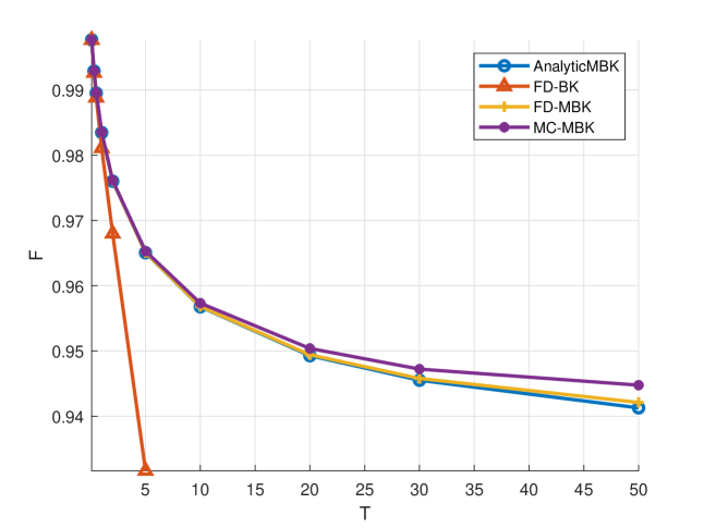
Figure 3: ZCB prices computed in the test by using Analytic, FD and Monte Carlo solutions.

Table 2: Relative error in bps between Analytic, FD and MC solutions in the test.

	T, years
Rel error	0.0833	0.3	0.5	1	2	5	10	20	30	50
Anal - FD	-0.0385	-0.0625	-0.0713	-0.0929	-0.2377	-0.2818	-0.5767	-1.4387	-2.8153	-8.7802
Anal - MC	-0.0844	-0.2447	-0.2803	-0.6167	-1.1802	-2.5238	-5.8173	-11.7015	-18.0272	-36.9372

The results obtained by all methods coincide with high accuracy. We compare the corresponding relative errors of those results in Table 2. Also, we compute the ZCB prices in the BK model for small $T$, so that $e^{z_{t}}\approx 1+z_{t}$. We choose $\bar{\theta}(t)_{BK}=\bar{\theta}(t)_{MBK}-1$. We show the result in Fig 3 as well. It can be seen that the BK ZCB prices agree with the corresponding MBK ZCB prices for $T<3$, which is due to the fact that $z$ is small.

As far as the performance of the methods is concerned, the elapsed time for computing all 10 ZCB bond prices by using the FD methods is 130 msec. For the analytics, since the only term under the integral in Eq. (3.3), which depends on $\tau$, is $e^{-(\omega^{2}+1/4)\tau}$, the other terms, including complex-valued Gamma and Whittaker functions, can be computed just once at the beginning of the script and then re-used. We calculate the integral by using the Simpson rule with 75 nodes; the elapsed time for getting all 10 ZCB prices is 55 msec. We note that internal Matlab implementation of the Whittaker functions is a bit slow as it relies on Simulink to compute them. In other programming languages, eg., C++ or python this is not an issue. Anyway, the performance of our method is on par with that of the forward FD solver, while the accuracy is higher. Moreover, we can further improve the accuracy of the integration by using higher-order quadratures while keeping the elapsed time similar. At the same time, for the FD method, this is problematic (but perhaps can be done by using Radial Basis Functions methods).

5 Conclusion

To summarize our findings, we have shown that in the current market environment, it is necessary to update the classical short-rate models. We introduced a useful extension of the popular BK model (the Verhulst model), which naturally produces prolonged periods of low rates and is more tractable. Finally, several complementary numerical and analytical methods to efficiently compute prices of the ZCB have been derived.

Appendix A Stylized facts about the BK model

The Black-Karasinski (BK) model was introduced in (Black and Karasinski, 1991), see also (Brigo and Mercurio, 2006) for a more detailed discussion. The BK is a one-factor short-rate model of the form

$$dz_{t} =k(t)[\theta(t)-z_{t}]dt+\sigma(t)dW_{t},\qquad r\in\mathbb{R},\ t\geq 0,$$ (A.1)

$$r_{t} =s(t)+Re^{z_{t}},\qquad r(t=0)=r_{0}.$$

Here $t$ is the time, $r_{t}$ is the short interest rate, $\kappa(t)>0$ is the constant speed of mean-reversion, $\theta(t)$ is the mean-reversion level, $\sigma(t)$ is the volatility, $R$ is some constant with the same dimensionality as $r_{t}$, eg., it can be 1/(1 year), $W_{t}$ is the standard Brownian motion. This model is similar to the Hull-White model but preserves the positivity of $r_{t}$ by exponentiating the OU random variable $z_{t}$. Frequently, practitioners add a deterministic function (shift) $s(t)$ to the definition of $r_{t}$ to address possible negative rates and be more flexible when calibrating the term-structure of the interest rates.

By the Itô’s lemma the short rate $\bar{r}_{t}=(r_{t}-s(t))/R$ in the BK model solves the following stochastic differential equation (SDE)

$$d\bar{r}_{t}=[k\theta(t)+\frac{1}{2}\sigma(t)^{2}-k\log\bar{r}_{t}]\bar{r}_{t}dt+\sigma(t)\bar{r}_{t}dW_{t}.$$ (A.2)

This SDE can be explicitly integrated. Let $0\leq s\leq t\leq T$, with $T$ being the maturity of a ZCB. Then $r_{t}$ can be represented as, (Brigo and Mercurio, 2006)

$$\bar{r}_{t}=\exp\left[e^{-k(t-s)}\log\bar{r}_{s}+k\int_{s}^{t}e^{-k(t-u)}\theta(u)du+\int_{s}^{t}\sigma(u)e^{-k(t-u)}dW_{u}\right],$$ (A.3)

and thus, conditionally on filtration $\mathcal{F}_{s}$ is lognormally distributed and always stays positive. The expectation ${\mathbb{E}}_{\mathbb{Q}}[r_{t}|\mathcal{F}_{s}]$ and variance $\mathrm{V}[r_{t}|\mathcal{F}_{s}]$ can be found analytically, (Brigo and Mercurio, 2006)

$${\mathbb{E}}_{\mathbb{Q}}[\bar{r}_{t}|\mathcal{F}_{s}] =\exp\left[e^{-k(t-s)}\log\bar{r}_{s}+k\int_{s}^{t}e^{-k(t-u)}\theta(u)du+\frac{1}{2}\int_{s}^{t}\sigma^{2}(u)e^{-2k(t-u)}du\right],$$ (A.4)

$$\mathrm{V}[\bar{r}_{t}|\mathcal{F}_{s}] =\exp\left[2e^{-k(t-s)}\log\bar{r}_{s}+2k\int_{s}^{t}e^{-k(t-u)}\theta(u)du\right]\left[e^{2\mathcal{I}(s,t)}-e^{\mathcal{I}(s,t)}\right].$$

However, in the BK model, the price $F(t,{\bar{r}})$ of a ZCB is not known in the closed form, since this model is not affine. Multiple good approximations have been developed in the literature using asymptotic expansions of various flavors; see, e.g., (Antonov and Spector, 2011; Capriotti and Stehlikova, 2014; Horvath et al., 2017), and also survey in (Turfus, 2020).

Appendix B An integral equation for the ZCB price in the BK model

It is known that, written in terms of $z$, the corresponding PDE for the ZCB price $F(t,z)$ reads, (Andersen and Piterbarg, 2010)

$$0 =\frac{\partial F}{\partial t}+\frac{\displaystyle 1}{\displaystyle 2}\sigma^{2}(t)\frac{\partial^{2}F}{\partial z^{2}}+\kappa(t)[\theta(t)-z]\frac{\partial F}{\partial z}-[s(t)+Re^{z}]V,$$ (B.1)

This equation should be solved subject to the terminal and boundary conditions, (Andersen and Piterbarg, 2010) (see also discussion in (Carr and Itkin, 2021))

$$F(T,z)=1,\qquad F(t,z)\Big{|}_{z\to\infty}=0.$$ (B.2)

Let us make the change of variables

$$x =a(t)z+b(t),\qquad\tau=\frac{1}{2}\int_{\nu}^{t}\sigma(m)^{2}e^{2\int_{\nu}^{m}\kappa(m)\,dm}\,dm,\qquad v(\tau,x)=e^{-\int_{\nu}^{t}s(t)\,dt}F(t,z),$$ (B.3)

$$a(t) =e^{\int_{\nu}^{t}\kappa(m)\,dm},\quad b(t)=-\int_{\nu}^{t}\theta(m)\kappa(m)e^{\int_{\nu}^{m}\kappa(m)\,dm}\,dm,.$$

where $\nu=const$. As is discussed below, this constant can be chosen to simplify the final expressions. With this change Eq. (B.1) can be transformed to

$$0 =\frac{\partial v}{\partial\tau}+\frac{\partial^{2}v}{\partial x^{2}}-\beta(t(\tau))e^{\bar{a}(t(\tau))x}v,$$ (B.4)

$$\beta(t) =\frac{2R}{\sigma(t)^{2}}e^{-2\int_{\nu}^{t}\kappa(m)\,dm-\frac{b(t)}{a(t)}},\quad\bar{a}(t)=\frac{1}{a(t)}$$

$$v(0,x) =1,\qquad\qquad\tau_{0}=\frac{1}{2}\int_{\nu}^{T}\sigma(m)^{2}e^{2\int_{\nu}^{m}\kappa(m)\,dm}\,dm.$$

Next, we apply the Fourier transform

$$w(\omega,\tau)=\int_{-\infty}^{\infty}v(\tau,x)e^{\mathrm{i}\mkern 1.0mu\omega x}dx,$$

to Eq. (B.4) to get the following problem

$$w_{\tau}-\omega^{2}w=\beta(\tau)\int_{-\infty}^{\infty}v(\tau,x)e^{\bar{a}(t)x}e^{\mathrm{i}\mkern 1.0mu\omega x}dx,\qquad w(\tau_{0},\omega)=2\pi\delta(\omega),$$ (B.5)

where $\delta(\omega)$ is the Dirac delta function. The solution of Eq. (B.5) reads

$$w=e^{\omega^{2}(\tau-\tau_{0})}w(\tau_{0},\omega)+\int_{\tau_{0}}^{\tau}e^{\omega^{2}(\tau-k)}\beta(k)\int_{-\infty}^{\infty}F(k,\zeta)e^{\bar{a}(k)\zeta-\int_{\nu(\tau)}^{t(\tau)}s(t)\,dt}e^{\mathrm{i}\mkern 1.0mu\omega\zeta}\,d\zeta\,dk.$$ (B.6)

Applying the inverse transform

$$v(\tau,x)=\frac{1}{2\pi}\int_{-\infty}^{\infty}w(\tau,\omega)e^{-\mathrm{i}\mkern 1.0mu\omega x}d\omega$$

yields

$$v(\tau,x) =1+\frac{1}{2\pi}\int_{-\infty}^{\infty}\int_{\tau_{0}}^{\tau}e^{\omega^{2}(\tau-k)}\beta(k)\int_{-\infty}^{\infty}v(k,\zeta)e^{\bar{a}(k)\zeta}e^{\mathrm{i}\mkern 1.0mu\omega(\zeta-x)}d\zeta\,dk\,d\omega$$

$$=1-\frac{1}{2\sqrt{\pi}}\int_{-\infty}^{\infty}\int_{\tau_{0}}^{\tau}\frac{\beta(k)e^{\zeta\bar{a}(k)}}{\sqrt{\tau-k}}e^{-\frac{(x-\zeta)^{2}}{4(\tau-k)}}v(k,\zeta)d\zeta dk,$$ (B.7)

where in the last line the change of variables $k\to-k,\ \tau\to-\tau$ was made.

Thus, the ZCB price solves the following two-dimensional Volterra integral equation of the second kind

$$v(\tau,x)=1-\frac{1}{2\sqrt{\pi}}\int_{-\infty}^{\infty}\int_{\tau_{0}}^{\tau}\frac{\beta(t(k))e^{\bar{a}(t(k))\zeta}}{\sqrt{\tau-k}}e^{-\frac{(x-\zeta)^{2}}{4(\tau-k)}}v(k,\zeta)d\zeta dk.$$ (B.8)

It can also be obtained by applying the Duhamel’s principle to Eq. (B.4).

Appendix C Methods for solving Eq. (B.8)

Eq. (B.8) is a two dimensional integral Volterra equation of the second kind. Various authors have proposed efficient numerical methods for solving this type of equations. These methods include the block-by-block method, collocation and iterated collocation methods, the differential transform method (DTM), Galerkin and spectral Galerkin methods, multi-step collocation methods, and several other, see (Torabi et al., 2019) and references therein. However, the complexity of the numerical methods (excluding the DTM) is at least $O(N^{3})$, where $N$ is the number of computational nodes. On the other hand, $N$ could be taken relatively small compared, e.g., with the corresponding finite-difference (FD) method, if the high order quadrature rules are used when approximating the integrals.

Also, when applying all the methods mentioned above, the infinite interval should be replaced with a finite one. Another change of variables can do this, e.g., $\zeta\mapsto\tanh(\zeta)$. Then another class of methods can be used where the unknown function $v(\tau,x)$ is expanded into series on some basis. This basis could be a set of orthogonal functions, or Taylor series, etc.

However, a quick estimation of the solution of Eq. (B.8) can be obtained along the lines of the reduced differential transform method (RDTM), (Abazari and Kilicman, 2013). The RDTM can be considered as an asymptotic solution of Eq. (B.8) around some time $t=t_{0}$. It can be constructed with arbitrary precision. It is worth mentioning that the RDTM can not be directly applied to Eq. (B.8) as the kernel in Eq. (B.8) depends on $\tau$ itself. Therefore, we propose a modification of the RDTM suitable to handle this situation as well.

Next, we briefly present basic definitions of the RDTM and some theorems from (Abazari and Kilicman, 2013) necessary to use this method for solving Eq. (B.8).

Consider a function of two variables $w(t,x)$, and suppose that it can be represented as a product of two single-variable functions $w(x,t)=f(x)g(t)$. The function $w(t,x)$ can be represented as

$$w(x,t)=\sum_{i=0}^{\infty}F(i)x^{i}\sum_{j=0}^{\infty}G(j)t^{j}=\sum_{i=0}^{\infty}\sum_{j=0}^{\infty}W_{j}(i)(i,j)x^{i}t^{j},$$ (C.1)

where $W(i,j)=F(i)G(j)$ is called the spectrum of $w(x,t)$.

To start with, we briefly present basic definitions of the RDTM and some theorems from (Abazari and Kilicman, 2013) necessary to use this method for solving Eq. (B.8).

Consider a function of two variables $w(t,x)$, and suppose that it can be represented as a product of two single-variable functions $w(x,t)=f(x)g(t)$. The function $w(t,x)$ can be represented as.

If the double sum in Eq. (C.1) is truncated to the $N$ terms in each variable, this expressions is the Poisson series of the input expression $w(x,t)$ with respect to the variables $(x,t)$ to order $N$ using the variable weights $W(i,j)$.

If $w(x,t)$ is an analytic function in the domain of interest, then the spectrum function

$$W_{k}(x)=\frac{1}{k!}\left[\frac{\partial^{k}}{\partial t^{k}}w(x,t)\right]_{t=t_{0}}$$ (C.2)

is called the reduced transformed function of $w(x,t)$. We use the notation where the lowercase $w(x,t)$ denotes the original function while the uppercase $W_{k}(x)$ stands for the reduced transformed function. The differential inverse transform of $W_{k}(x)$ is defined as

$$w(x,t)=\sum_{k=0}^{\infty}W_{k}(x)(t-t_{0})^{k}.$$ (C.3)

Combining Eq. (C.2) and Eq. (C.3) one can get

$$w(x,t)=\sum_{k=0}^{\infty}\frac{1}{k!}\left[\frac{\partial^{k}}{\partial t^{k}}w(x,t)\right]_{t=t_{0}}(t-t_{0})^{k}.$$ (C.4)

To proceed, we need the following fragment of Theorem 7 in (Abazari and Kilicman, 2013)

Theorem 1.

Assume that $U_{k}(x),H_{k}(x)$ and $W_{k}(x)$ are the reduced differential transforms of the functions $u(x,t),h(x,t)$ and $w(x,t)$, respectively. If

$$w(x,t)=\int_{t_{0}}^{t}\int_{x_{0}}^{x}h(y,z)u(y,z)dydz,$$ (C.5)

then

$$W_{k}(x)=\frac{1}{k}\int_{x_{0}}^{x}\left(\sum_{\nu=0}^{k-1}H_{\nu}(y)U_{k-\nu-1}(y)\right)dy,\qquad k=1,2,\ldots.$$ (C.6)

Proof.

See (Abazari and Kilicman, 2013). ∎

Now one can observe that Eq. (B.8) actually has the form of Eq. (C.5) with $x=\infty,x_{0}=-\infty,t_{0}=0$, and thus

$$u(k,\zeta) =-\beta(t(k))e^{\zeta\bar{a}(t(k))}\frac{1}{2\sqrt{\pi(\tau-k)}}e^{-\frac{(x-\zeta)^{2}}{4(\tau-k)}}.$$ (C.7)

Our modification of the RDTM consists in eliminating the definition in Eq. (C.2) for the function $u(k,\zeta)$. Then, based on the definition of the reduced differential transform in Eq. (C.2), we get

$$U_{0}(s,\zeta) =-\beta(t(s))e^{\zeta\bar{a}(t(s))}\frac{1}{2\sqrt{\pi(\tau-s)}}e^{-\frac{(x-\zeta)^{2}}{4(\tau-s)}},$$ (C.8)

$$U_{1}(s,\zeta) =-\int_{0}^{s}\beta(t(k))e^{\zeta\bar{a}(t(k))}\frac{1}{2\sqrt{\pi(s-k)}}e^{-\frac{(x-\zeta)^{2}}{4(s-k)}}dk,$$

and so on.

Let us denote the reduced differential transform of $v(\tau,x)$ as $W_{k}(x)$. From Eq. (B.8) it follows that $W_{0}(x)=1$, as the double integral vanishes at $\tau=0$, and the following properties of the RDT hold

$$w_{k}(x) =u_{k}(x)\pm v_{k}(x)\quad \longmapsto\quad W_{k}(x)=U_{k}(x)\pm V_{k}(x),$$

$$w(x,t) =A=const,\quad \longmapsto\quad W_{0}(x)=1,\quad W_{k}(x)=0,\ k>0,$$

Then from Eq. (C.6), and Eq. (C.8) we have

$$W_{1}(x)=\int_{0}^{\tau}\int_{-\infty}^{\infty}W_{0}(s,\zeta)U_{0}(s,\zeta)d\zeta ds=\int_{0}^{\tau}e^{{\bar{a}}(s)({\bar{a}}(s)(\tau-s)+x)}ds.$$ (C.9)

The next iteration reads

$$W_{2}(x) =\int_{0}^{\tau}\int_{-\infty}^{\infty}\left[W_{1}(\zeta)U_{0}(\zeta)+W_{0}(\zeta)U_{1}(\zeta)\right]d\zeta\,ds=I_{1}+I2,$$ (C.10)

$$I_{1} =\int_{0}^{\tau}\int_{0}^{s}\beta(k)\beta(s)e^{a(k)(2a(s)(\tau-s)+x)+a(k)^{2}(\tau-k)+a(s)(a(s)(\tau-s)+x)}dk\,ds,$$

$$I_{2} =-\int_{0}^{\tau}\int_{0}^{s}\beta(t(k))e^{\zeta\bar{a}(t(k))}\frac{1}{2\sqrt{\pi(s-k)}}e^{-\frac{(x-\zeta)^{2}}{4(s-k)}}dk\,ds,$$

etc.

Once all the terms $W_{k}(x),\ k=1,\ldots,N$ are found, the final representation of the solution follows from the inverse formula Eq. (C.3) changed according to our modification of the RDTM

$$v(\tau,x)=\sum_{k=0}^{N}W_{k}(x).$$ (C.11)

The time-integrals in Eq. (C.9), Eq. (C.10) can be computed either numerically, or analytically if functions ${\bar{a}}(\tau),\beta(\tau)$ could be expanded into series on $\tau$ around some $\tau_{0}$. In the latter case the method becomes almost identical to the original RDTM. When doing so, one has to remember that derivatives of $a(\tau),\beta(\tau)$ are the derivatives on $\tau$ while the definitions of these functions in Eq. (B.3) are given in terms of $t=t(\tau)$. The latter map is also given in Eq. (B.3).

C.1 Numerical example

To test the RDTM as applied to our problem, we solve Eq. (B.8) by using the modified RDTM described in Section C. Here we use the following explicit form for $\kappa(t),{\tilde{\theta}}(t),\sigma(t)$

$$\kappa(t)=\kappa_{0},\qquad{\tilde{\theta}}(t)={\tilde{\theta}}_{0}e^{\theta_{1}t},\qquad\sigma(t)=\sigma_{0}e^{-\sigma_{1}t},$$ (C.12)

where $\kappa_{0},\theta_{0},\sigma_{0},\theta_{1},\sigma_{1}$ are constants. We also assume $s(t)=0$, and $R=1$. With these definitions, we have

$$a(t) =e^{-k(t-\nu)},\quad b(t)=\left(e^{\theta_{1}\nu}-e^{t(\kappa_{0}+\theta_{1})-\kappa_{0}\nu}\right)\frac{\kappa_{0}\theta_{0}}{\kappa_{0}+\theta_{0}},$$ (C.13)

$$\beta(t) =\frac{2}{\sigma^{2}_{0}}\exp\left[\frac{2\theta_{0}}{\kappa_{0}+\theta_{1}}\left(e^{\theta_{1}t}-e^{\nu(\theta_{1}+\kappa_{0})-\kappa_{0}t}\right)+2t(\sigma_{1}-\kappa_{0})+2\kappa_{0}\nu\right],$$

$$t(\tau) =\frac{\log\left(e^{-2\sigma_{1}\nu}-\frac{2\tau(\kappa_{0}-2\sigma_{1})}{\sigma^{2}_{0}}\right)+\kappa_{0}\nu}{\kappa_{0}-2\sigma_{1}}.$$

Table 3: Parameters of the test.

$r_{0}$	$\kappa_{0}$	$\theta_{0}$	$\sigma_{0}$	$\theta_{1}$	$\sigma_{1}$
0.01	1.0	0.05	0.5	0.2	0.2

Table 4: Prices of ZCB bonds with different maturities computed by using the modified RDTM with 1 and 2 terms, and the FD difference method.

	ZCB price, $
T	0.0833	0.3	0.5	1.0	2.0	5.0
FD	0.9990	0.9938	0.9839	0.9216	0.6201	0.0444
RDTM-1	0.9990	0.9950	0.9887	0.9617	0.5857	0.2477
RDTM-2	0.9990	0.9949	0.9883	0.9587	0.6186	0.6087
	Difference with the FD method, %
T	0.0833	0.3	0.5	1.0	2.0	5.0
FD	0.0000	0.0000	0.0000	0.0000	0.0000	0.0000
RDTM-1	0.0047	0.1142	0.4907	4.3563	-5.5489	457.6831
RDTM-2	0.0042	0.1039	0.4494	4.0263	-0.2491	1270.3588

We present the model parameters for this test in Table 3. We run the test for a set of maturities $T\in[1/12,0.3,0.5,1,2,5]$. We show the corresponding ZCB prices in Table 4. As a benchmark, we use the solution of Eq. (B.1) obtained by using the FD method described above. The modified RDTM provides reasonable accuracy for small maturities (up to 2 years), while for $T>2$, one or two terms in the expansion are insufficient to get the correct price. Therefore, for larger $T$, the Eq. (B.8) has to either be solved numerically or more terms should be taken in the RDTM.

Note, that there are at least two choices for $\nu$ in Eq. (B.3): $\nu=0$ and $\nu=T$. We found that for small $T$ the choice $\nu=0$ provides slightly better results, while for $T>1$ it is better to use $\nu=T$.

Also, note that this method, in some sense, is similar to that in (Capriotti and Stehlikova, 2014). However, we solve an integral equation instead of a PDE in (Capriotti and Stehlikova, 2014). Besides, there is a difference in parametrization, since we assume that all the parameters are time-dependent. In contrast, in (Capriotti and Stehlikova, 2014), all model parameters are constant.

As far as the performance of the RDTM is concerned, we compared it with the performance of the FD method applied to the forward equation (the forward analog of Eq. (B.1). The elapsed time of getting the ZCB prices by solving such the equation is 40 msec while using the RDTM even with the numerical computation of all integrals in Eq. (C.10) takes 13 msec. Therefore, this method allows fast calculation of ZCB prices in the time-dependent BK model for $T<2$.

References

• Abazari and Kilicman (2013) R. Abazari and A. Kilicman. Numerical Study of Two-Dimensional Volterra Integral Equations by RDTM and Comparison with DTM. Abstract and Applied Analysis, (929478), 2013.
• Abramowitz and Stegun (1964) M. Abramowitz and I. Stegun. Handbook of Mathematical Functions. Dover Publications, Inc., 1964.
• Andersen and Piterbarg (2010) L.B.G. Andersen and V.V. Piterbarg. Interest Rate Modeling. Number v. 2 in Interest Rate Modeling. Atlantic Financial Press, 2010. ISBN 9780984422111.
• Antonov and Spector (2011) A. Antonov and M. Spector. General short-rate analytics. Risk, pages 66–71, 2011.
• Bacaer (2011) N. Bacaer. A short history of mathematical population dynamics, chapter 6, pages 35–39. Springer-Verlag, London, 2011. ISBN 978-0-85729-114-1.
• Black and Karasinski (1991) F. Black and P. Karasinski. Bond and option pricing when short rates are lognormal. Financial Analysts Journal, pages 52–59, 1991.
• Brigo and Mercurio (2006) D. Brigo and F. Mercurio. Interest Rate Models – Theory and Practice with Smile, Inflation and Credit. Springer Verlag, 2nd edition, 2006.
• Capriotti and Stehlikova (2014) L. Capriotti and B. Stehlikova. An Effective Approximation for Zero-Coupon Bonds and Arrow-Debreu Prices in the Black-Karasinski Model. International Journal of Theoretical and Applied Finance, 17(6):1650017, 2014.
• Carr and Itkin (2021) P. Carr and A. Itkin. Semi-closed form solutions for barrier and American options written on a time-dependent Ornstein Uhlenbeck process. Journal of Derivatives, Fall, 2021.
• Carr et al. (2020) P. Carr, A. Itkin, and D. Muravey. Semi-closed form prices of barrier options in the time-dependent cev and cir models. Journal of Derivatives, 28(1):26–50, 2020.
• Chen (2010) S. Chen. Decisions modeling the dynamics of commodity prices for investement decisions under uncertainty. PhD thesis, University of Waterloo, Ontario, Canada, 2010.
• Cohen Jr. (1940) A.C. Cohen Jr. The numerical computation of the product of conjugate imaginary gamma functions. Ann. Math. Statist., 11(2):213–218, 1940.
• Giet et al. (2015) J.S. Giet, P. Vallois, and S. Wantz-Mezieres. The logistic sde. Theory of Stochastic Processes, 20(36):28–62, 2015.
• Gradshtein and Ryzhik (2007) I.S. Gradshtein and I.M. Ryzhik. Table of Integrals, Series, and Products. Elsevier, 2007.
• Halperin and Feldshteyn (2018) I. Halperin and I. Feldshteyn. Market self-learning of signals, impact and optimal trading:invisible hand inference with free energy, May 2018. SSRN:3174498.
• Horvath et al. (2017) B Horvath, A. Jacquier, and C. Turfus. Analytic option prices for the black-karasinski short rate model, 2017. URL https://papers.ssrn.com/sol3/papers.cfm?abstract_id=3253833. SSRN: 3253833.
• Itkin (2017) A. Itkin. Pricing derivatives under Lévy models. Number 12 in Pseudo-Differential Operators. Birkhauser, Basel, 1 edition, 2017.
• Itkin and Muravey (2020) A. Itkin and D. Muravey. Semi-closed form prices of barrier options in the Hull-White model. Risk, December 2020.
• Lipton (2001) A. Lipton. Mathematical Methods For Foreign Exchange: A Financial Engineer’s Approach. World Scientific, 2001.
• Lipton and Kaushansky (2020) A. Lipton and V. Kaushansky. On three important problems in mathematical finance. The Journal of Derivatives. Special Issue, 2020.
• Londono and Sandoval (2015) J.A. Londono and J. Sandoval. A new logistic-type model for pricing european options. SpringerPlus, (4):762, December 2015.
• Rudebusch (2018) G.D. Rudebusch. A review of the fed’s unconventional monetary policy. FRBSF Economic Letter, (27), December 2018.
• Temme (1978) N.M. Temme. Uniform asymptotic expansions of confluent hypergeometric functions. J. Inst. Maths Applies, 22:215–223, 1978.
• Torabi et al. (2019) S.M. Torabi, A. Tari, and S. Shahmorad. Two-step collocation methods fortwo-dimensional volterra integral equationsof the second kind. Journal of Applied Analysis, 25(1):1–11, 2019.
• Turfus (2020) C. Turfus. Analytic swaption pricing in the black-karasinski model, February 2020. URL https://papers.ssrn.com/sol3/papers.cfm?abstract_id=3253866. SSRN: 3253866.
• Verhulst (1838) P.F. Verhulst. Notice sur la loi que la population suit dans son accroisseement. Correspondance mathematique et physique, 10:113–121, 1838.
\appendixpage