Exploiting Weight Redundancy in CNNs: Beyond Pruning and Quantization

Abstract.

Pruning and quantization are proven methods for improving the performance and storage efficiency of convolutional neural networks (CNNs). Pruning removes near-zero weights in tensors and masks weak connections between neurons in neighbouring layers. Quantization reduces the precision of weights by replacing them with numerically similar values that require less storage. In this paper we identify another form of redundancy in CNN weight tensors, in the form of repeated patterns of similar values. We observe that pruning and quantization both tend to drastically increase the number of repeated patterns in the weight tensors.

We investigate several compression schemes to take advantage of this structure in CNN weight data, including multiple forms of Huffman coding, and other approaches inspired by block sparse matrix formats. We evaluate our approach on several well-known CNNs and find that we can achieve compaction ratios of 1.4$\times$ to 3.1$\times$ in addition to the saving from pruning and quantization.

1. Introduction

Deep Neural Networks are hugely successful in artificial intelligence applications such as computer vision, natural language processing, and robotics. Deep networks with a large number of layers and many thousands of trainable parameters within in each layer can achieve remarkable inference accuracy. However, these networks require large amounts of computation, memory and energy (Han et al., 2015b) for inference. These heavy requirements are a major barrier to the deployment of deep learning, especially on resource-constrained mobile or embedded systems.

Although a large number of parameters can help to bring greater classification accuracy, researchers have found that, in practice, parameters have a great deal of redundancy.

In particular, many trained weights are close to zero, and it is often possible to prune these small weights (by setting them to zero) resulting in a sparse weight matrix (Iandola et al., 2016; Mao et al., 2017; Luo et al., 2017).

Weights which are not close to zero can still be quantized to a lower precision to reduce storage requirements. Quantization works by representing fewer digits of, or eliminating, the fractional part of each weight. A number of schemes have been proposed for both encoding and quantization of CNN weights (Judd et al., 2017; Gysel et al., 2016; Vanhoucke et al., 2011).

Pruning and quantization can be enormously successful in reducing the number and precision of weight parameters in DNNs. Researchers have found that pruning can reduce the number of weights by up to 90% (Han et al., 2015b).

Despite the success of pruning and quantization, there is still a need to reduce the size of weight tensors in DNNs. High-performance and efficient inference on edge devices is becoming crucial (Franklin, 2017) to make possible applications where response time is critical (e.g. detection of pedestrians or obstacles in an automotive context). However, edge devices are heavily constrained, particularly in terms of available memory for storing weight tensors.

By examining weight tensors from various DNNs, we observed a great deal of redundancy in the non-zero weights. We found that after pruning and quantization, similar patterns of weights arise again and again, in both the convolutional and fully connected layers of CNNs. This redundancy in convolutional layers is particularly important because pruning is much less effective in convolutional than fully-connected layers (Mao et al., 2017).

A typical approach to exploiting structural redundancy in data to reduce storage requirements is to use a compression scheme to store data in memory. Element-wise Huffman coding has previously been used to compress CNN weight data (Han et al., 2015a), but other compression approaches seem equally promising, particularly since the redundancy we observed in weight data appears at a range of granularities, from single elements to whole blocks of repeated weight data.

Contributions

We make the following contributions:

• We study the prevalence of repeated patterns in CNN weight tensors, and show that there is significant redundancy even after pruning and quantization.

• We evaluate both element-wise and block Huffman coding for weight compression.

• We propose and evaluate a novel model compaction scheme that exploits redundancy in weight tensors represented in a block sparse format.

• We evaluate our scheme and find that we achieve reductions of 1.4$\times$ to 3.1$\times$ in addition to the savings from pruning and quantization.

2. Related Work

DNN inference is often most useful in real-time (Han et al., 2015a) or resource-constrained (Ding et al., 2017; Yang et al., 2017a) contexts. However, the computational complexity and exceptionally large number of parameters in deep neural networks presents challenges around execution time, data movement, and memory capacity in these contexts (Denil et al., 2013). Pruning and quantization both aim to reduce the number of parameters in deep networks. Since the complexity of most network layers is a function of the number of parameters, a reduction in computation (typically stated as the number of multiply-accumulate or MAC operations) accompanies parameter reduction (Yu et al., 2017).

2.1. Pruning

Researchers have found that not all parameters make an equal contribution to the output of any one DNN layer. Similarly, some connections between layers have little impact on the output of the overall network. Removing (pruning) these unimportant connections can save significant storage and reduce execution time and has been widely advocated as an efficient method to reduce the number of parameters (Yang et al., 2017b; Anwar et al., 2017; Guo et al., 2016; Lin et al., 2017; He et al., 2017).

Much work on pruning focuses on identifying which weights can be pruned with least effect on the classification accuracy of the overall network. Various metrics, such as second-order derivative (Hassibi and Stork, 1992; LeCun et al., 1989), Average Percentage of Zeros (Hu et al., 2016), absolute values (Li et al., 2016; Han et al., 2015b), and output sensitivity (Engelbrecht, 2001), have been proposed to guide the pruning process.

Pruning results in a sparse weight matrix, which can be compacted by storing only the non-zero values (Kepner et al., 2017). Common sparse matrix representations (Saad, 2003) include coordinate (COO) format, where each non-zero value is stored with its row and column coordinate; and compressed sparse row (CSR) where non-zero values from the same row are grouped together, and only the column index is stored for each non-zero.

These fine-grain sparse matrix formats save space, but modern CPUs and GPUs provide vector SIMD/SIMT instructions that are much better suited to operating on dense matrix formats. Using a fine-grained sparse format typically reduces computational performance versus similarly sized dense matrices (Yu et al., 2017), making high-performance implementation of DNN layers more difficult.

To overcome this problem, alternative sparse matrix representations have been developed, where the smallest granularity is a small dense block of data rather than a single matrix element. The most widely-used of these formats is block sparse row (BSR) (Williams et al., 2007), which is similar to CSR but contains small dense blocks rather than indidual non-zeros.

2.2. Quantization

One way to reduce the storage required for non-zero values that remain after pruning is to use approximate values. Quantization is typically used for inference, since at this stage the weight values are frozen, and do not need to track updates in high precision, as they do during the network training process.

Rather than storing each value in the full precision that is used for training, such as 32-bit floating point, a smaller size such as 16-bits (Judd et al., 2017), 8-bits (Gysel et al., 2016; Vanhoucke et al., 2011), or 4-bits (Moons and Verhelst, 2016) can be used for inference.

To convert the full-precision trained weights to lower-precision values for inference, some quantization scheme is needed. Provided the quantization is not too severe, the loss in inference accuracy is typically small (Sze et al., 2017), but the saving in space is large. For example, quantizing from 32-bit floating point to 8-bit integer reduces the size of non-zero values by a factor of four.

2.3. Encoding

To further reduce the memory requirements for weight data, various encoding schemes can be used. For example, Han et al. (Han et al., 2015a) use Huffman coding to compress the weight data even further. Huffman coding works by building a dictionary of values in the input data, and replacing instances of each particular value with that value’s label from the dictionary. The most frequent values are assigned the shortest labels. Using this tactic, we can represent elements in the weight matrix using labels whose size is related to the number of unique values.

3. Redundant Patterns

When we examine the weights of a trained CNN, we observe many similar patterns. The training process seldom creates patterns that are identical to the last bit of precision in every weight. However, pruning and quantization both reduce the number of unique weight values appearing in the tensors. Two patterns that are very similar before pruning and quantization often become identical afterwards. The result is a large number of repeated patterns in the weight tensors.

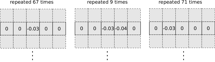
Figure 1. Repeated kernel-width vectors in the second convolutional layer of LeNet-5, after pruning and quantization

To illustrate this phenomenon, Figure 1 shows an example of the weight tensor of the second convolutional layer of LeNet-5 after pruning and quantization. In this convolutional layer the kernel size of is $5\times 5$, and for the purposes of illustration we show the kernel tensor as a 2D matrix of width 5. Thus, each row of the matrix is one row of a $5\times 5$ kernel. When viewed in this way, we can identify rows of the matrix that appear more than once. Figure 1 shows three rows that appear 67, 9, and 71 times respectively. These repeated rows offer opportunities for compacting the kernel tensor to reduce memory requirements.

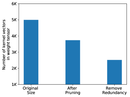
Figure 2. Parameter reduction in LeNet-5 by pruning followed by compression of redundant vectors.

In practice, the number of redundant vectors is large. Figure 2 shows the storage saving by keeping just a single copy of each repeated vector. The first bar in Figure 2 shows the overall number of kernel-width vectors in the second convolutional layer of LeNet-5. The second bar shows the number of vectors after kernel-wise pruning and quantization. Finally, the third bar shows the number of vectors remaining after removing repeated copies. As we can see in this example, eliminating repeated patterns can provide an additional saving of around 2$\times$ when compared with pruning and quantization alone.

An important question is why so much redundancy arises between vectors of trained weights. It can be difficult to fully understand why specific parameters within a CNN receive a particular value during training. However, a partial explanation is that CNNs learn to replicate aspects of classical machine vision techniques.

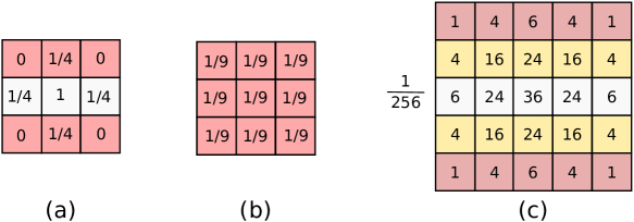
Figure 3. Kernels used for image processing (González and Woods, 2008): (a) Edge detection (b) Box blur (c) Gaussian blur. As highlighted by rows, kernel-vector redundancy exists within kernels.

Figure 3 shows three classical machine vision filters that have been designed by humans to perform edge detection and image blurring. It is notable that all three kernels are symmetric along one or more axes. The symmetry of these kernels introduces redundancies in a granularity of kernel-width. If we remove repeated horizontal vectors from the kernels in Figure 3, then the remaining values occupy just two-thirds, one-third, and three-fifths of the orginal size respectively.

The kernel values in a trained DNN are not designed by humans, but instead emerge from the training process. The CNN learns them iteratively by back propagation and stochastic gradient descent (SGD). However, many of the same kernel features that are designed by humans for classical machine vision are also likely to emerge from the training process. These regular features are likely to appear alongside other, more complex features that allow CNNs to exceed the accuracy of classical vision techniques. Thus, we expect to see symmetries emerge within trained kernels that can lead to repeated rows within the kernel. Further, the same sub-features may appear across multiple patterns leading to further redundancy. By keeping just one copy of these common sub-features and sharing that copy among multiple instances, significant space savings become possible. In the next section we explain how block sharing can reduce the size of CNN models using a method inspired by block sparse row (BSR) format for representing sparse matrices.

4. Model Compaction with Block Sharing

Our block sharing method builds upon existing methods of network pruning and quantization to further reduce the size of the model. Our method has four main steps, which are shown in Figure 4.

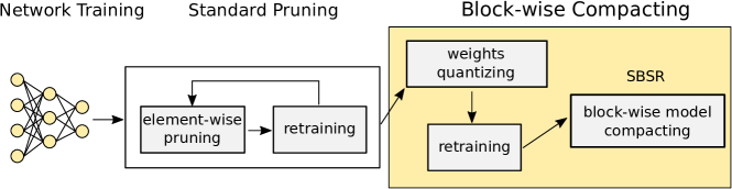
Figure 4. Flow of our DNN model compaction method

In the first step we prune the network to replace existing values with zero where possible. We use the Scapel (Yu et al., 2017) pruning method, which iteratively masks out values in the weight tensors and then retrains the network to recover accuracy. The retraining step is critical to the accuracy of the pruned model. We iteratively prune and retrain in a similar way to other state-of-the-art (Anwar et al., 2017; Li et al., 2016; Hu et al., 2016) pruning techniques.

In the second step, we quantize the remaining non-zero weights to reduce their precision, and thus the space required for storage. Our quantization factor is linked to the threshold value that is used in pruning, so that losses in precision are similar for both processes. After quantization, the network is again retrained to recover the accuracy lost by reducing the precision of the weights. Finally, we scan the weight tensors layer-by-layer to detect repeated weight blocks and replace them with references to a single shared copy of the block.

4.1. Network Pruning

Similar to the standard pruning methods, the network is first trained in full 32-bit floating point precision. The model is then iteratively pruned and retrained. In the pruning step, a theshold value is selected and all weights whose absolute value is below the threshold are tentatively masked to zero. The network is then retrained to improve accuracy. In the forward step, masked weights are treated as zeroes, but during back-propagation the original, non-zero value is updated. Thus, a value that is pruned in one iteration may recover in the next round of retraining.

One important question is the level of granularity at which pruning occurs. One approach is to prune at the level of individual weights within a tensor. Another method is to prune entire blocks of weights, or indeed entire kernels or channels. In general, finer-grain pruning eliminates large numbers of weights with little impact on the accuracy of the DNN, whereas a similar level of coarser-grain pruning tends to have a large impact on accuracy (Mao et al., 2017). We prune at a fine grain to maintain accuracy, but store the resulting tensors in a block-sparse row (BSR) format which offers greater opportunity for efficient implementation on modern CPUs and GPUs (Yu et al., 2017).

4.2. Quantization and precision reduction

The remaining non-zero weights are quantized and their precision is reduced. An assumption of our pruning approach is that values smaller than the threshold have only a minor impact on the result of the CNN and can be safely removed. Similarly, in our quantization step we may full-precision values to a nearby value that is representable in lower precision. In our experiments we use 32-bit precision for the original values, and 16-bit for the quantized values.

A question that is often ignored in discussions of quantization is the rounding of full-precision values that fall between two representable lower-precision values. The easiest strategy is to simply truncate the lower bits of such values, but rounding to the nearest representable value gives slightly better accuracy. The rounding strategy also has an impact on the patterns of values that appear in the weight tensors, and in the number of repeated patterns. We investigate this in more detail in Section 5.

Pruning and quantization are conceptually similar processes, in the sense that they replace an exact value with a nearby approximation. Just as we retrain after pruning, to maintain the accuracy of the CNN we must also retrain after quantization, as shown in Figure 4. This process tunes the quantized values and the bias to recover the accuracy of the model.

4.3. Block sharing

After pruning and quantization we represent the resulting matrix in block sparse row (BSR) format (see Figure 5). In contrast to fine-grain sparse formats, such as compressed sparse row (CSR) format, BSR uses dense blocks of values containing at least one non-zero rather than individual non-zeros. BSR has two main advantages: it allows faster CPU SIMD and GPU implementations, and by sharing the row and column coordinates between multiple separate values it allows more compact matrix representations (Mao et al., 2017).

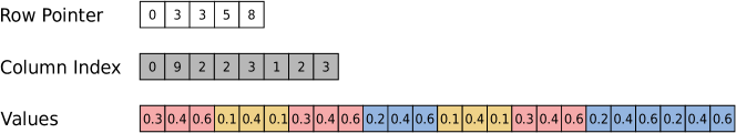
Figure 5. Classic BSR format

Although BSR can result in more compact sparse matrix representations, our results in this current paper show that it nonetheless contains a great deal of redundancy. As we show in Section 5 many instances of the same dense blocks occur many times in BSR format. We apply block-wise sharing to the matrix in BSR format to eliminate this redundancy. We propose a new matrix format which we call shared-block sparse row (SBSR) format, which allows repeated blocks to be shared between different entries in the sparse matrix.

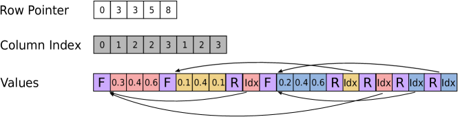
Figure 6. SBSR format (ours)

Figure 6 shows our SBSR format. For blocks that appear for the first time, the format is similar to BSR. The values of the block are stored in a block vector, which exists alongside the row pointers and column indices. However, when a block appears for a second or subsequent time, the values of the block are not represented. Instead, a reference is inserted into the block matrix, which refers back to the previous location where that block appeared. Thus, the values of a repeated block appear only in the first appearance of that block, and subsequent appearances are replaced with an reference to the shared block. Note that this format also requires a flag to indicate whether the block appears for the first time (F in Figure 6) or a repeat appearance (R). This flag can be represented as a single bit.

5. Experimental evaluation

To evaluate our method we modified the Scalpel (Yu et al., 2017) framework for pruning and retraining DNNs using an AMD Linux server with two Nvidia GTX 1080Ti GPUs. We set the pruning thresholds to achieve target levels of sparsity, and added a new quantization phase to reduce the precision of trained weights. Finally, we build the resulting matrices in block sparse row (BSR) and our own shared-block sparse row (SBSR) formats.

Figure 7 shows the factor reduction in size from sharing repeated blocks rather than representing them each time they appear. We explore three levels of sparsity: 40%, 60% and 80%. Mao et al. (Mao et al., 2017) found that pruning convolution kernels beyond 40%-60% sparsity typically results in large losses in accuracy. In contrast, fully connected layers can commonly be pruned to 80%-90% with negligible loss of accuracy.

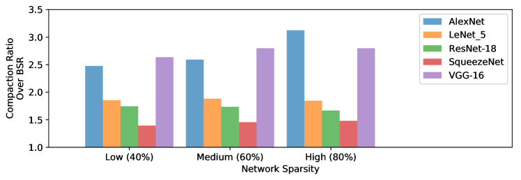
Figure 7. Improvement of SBSR over BSR on CNNs for 40%, 60% and 80% sparsity.

Figure 7 shows that significant savings in storage are possible using our shared-block strategy. For AlexNet, the saving is a factor of around 2.4, 2.6 and 3.2 (which corresponds to a reduction of around 58%, 62% and 69%) in the size of the represented matrix. The savings for other trained CNNs are smaller, but in all cases the savings are positive and significant.

(1) $$\small Size_{BSR}={BSR_{idx}+BSR_{blocks}}$$

(2) $$\small Size_{SBSR}={S_{flag}+S_{block\_pointer}+S_{idx}+S_{unique\_blocks}}$$

The memory requirement of BSR and SBSR formats are calculated according to Equations 1 and 2 respectively, where $B_{idx}$ and $S_{idx}$ represent the storage for the BSR format column and row indices, $BSR_{blocks}$ the storage for the all non-zero tensor blocks, $S_{flag}$ the memory for storing the flag that indicates if the following block is repeated or not, and $S_{unique\_blocks}$ is the size of all the unique blocks that are present in the sparse tensor.

Table 1. Breakdown of the compaction ratio by layer for AlexNet for 60% sparsity

Layer	Dense	Sparse Matrix	Sparse Matrix	Compaction
	Matrix	(After Compaction)	(over BSR)	Ratio
conv1	90.75kB	40.03kB	38.19kB	1.05x
conv2	1200kB	626.7kB	386.9kB	1.62x
conv3	2.53MB	1.38MB	0.80MB	1.73x
conv4	3.38MB	1.12MB	0.67MB	1.67x
conv5	2.25MB	0.68MB	0.41MB	1.66x
fc6	144.0MB	83.60MB	28.69MB	2.91x
fc7	64.00MB	36.98MB	16.12MB	2.29x
fc8	15.63MB	8.51MB	4.20MB	2.03x

Table 1 shows a more detailed breakdown of the compaction that is achieved in different layers of AlexNet. We see that the level of block sharing in the first layer, which is an $11\times 11$ convolution, is very small. However, the subsequent convolution layers, which use much smaller kernels, offer much great opportunity for sharing blocks. Note that for convolution layers, we use a block size that corresponds to one row of a convolution kernel (i.e. a vector of length 11 for an $11\times 11$ kernel). The savings from sharing in the fully-connected layers are even larger. Table 2 shows the same data for VGG16. There is a correlation between the size of the matrix, and thus the number of blocks, and the opportunities for sharing identical blocks.

Table 2. Breakdown of the compaction ratio by layer for VGG16 for 60% sparsity

Layer	Dense	Sparse	Sparse Matrix	Compaction Ratio
	Matrix	Matrix	(After Compaction)	(over BSR)
conv1_1	6.75kB	3.32kB	3.12kB	1.06x
conv1_2	144.0kB	71.93kB	50.10kB	1.44x
conv2_1	288.0kB	146.7kB	95.57kB	1.53x
conv2_2	576.0kB	203.5kB	179.5kB	1.13x
conv3_1	1.13MB	0.57MB	0.34MB	1.70x
conv3_2	2.25MB	1.17MB	0.68MB	1.74x
conv3_3	2.25MB	1.18MB	0.68MB	1.74x
conv4_1	4.50MB	2.43MB	1.37MB	1.77x
conv4_2	9.00MB	4.78MB	2.69MB	1.76x
conv4_3	9.00MB	4.48MB	2.53MB	1.77x
conv5_1	9.00MB	4.75MB	2.64MB	1.80x
conv5_2	9.00MB	4.68MB	2.58MB	1.81x
conv5_3	9.00MB	4.51MB	1.51MB	2.99x
fc6	392.0MB	225.7MB	72.51MB	3.11x
fc7	64.00MB	37.30MB	14.99MB	2.49x
fc8	15.63MB	8.73MB	4.65MB	1.88x

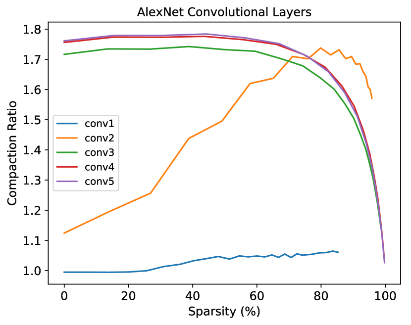
(a) Convolutional layers

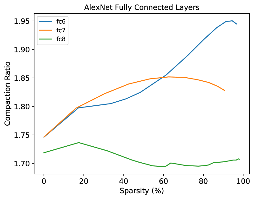
(b) Fully connected layers

Figure 8. Compaction per layer for AlexNet

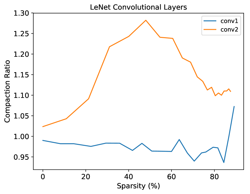
(a) Convolutional layers

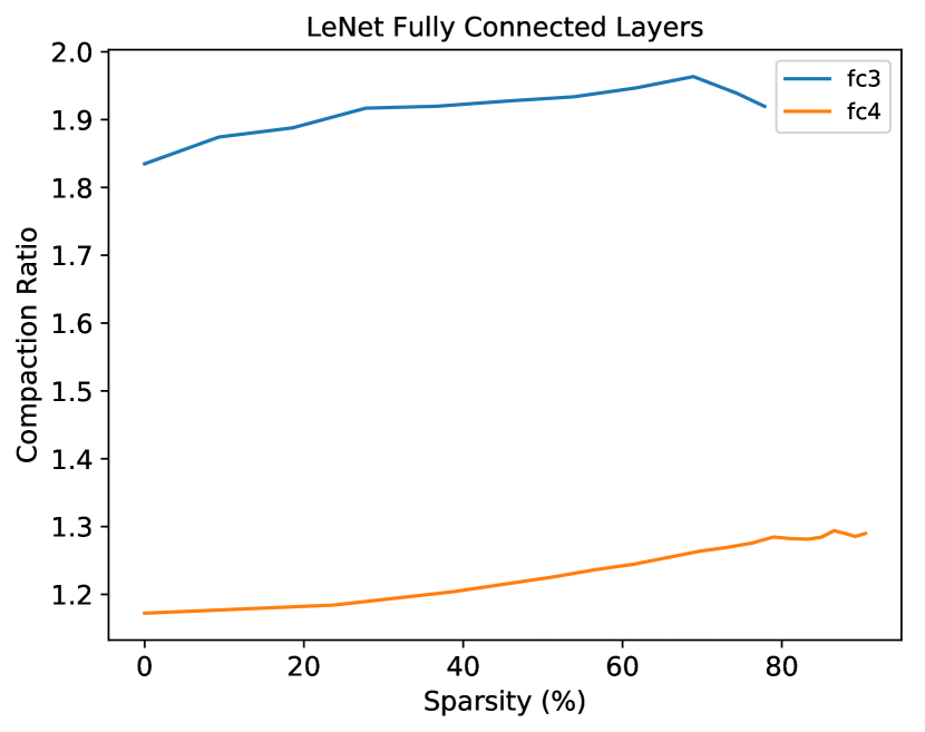
(b) Fully connected layers

Figure 9. Compaction per layer for LeNet

Figure 8 shows another view of the compaction ratio for different layers of AlexNet. Figure 8(a) shows the compaction ration for AlexNet’s five convolution layers. The rows of the $11\times 11$ kernels of the conv1 layer provide few opportunities for sharing. The rows are too long, the values are too diverse, and the number of the kernels too small for many repeated rows to appear. In contrast, the level of sharing increases rapidly as sparsity increases in the weights for layer conv2. As more small values are replaced with zero, small differences between blocks tend to disappear and more sharing becomes possible. In contrast, convolution layers 4, 5, and 6 have a great number of repeated blocks even without pruning. The compaction ratio for these layers falls with very high levels of sparsity simply because blocks that might otherwise be duplicates are eliminated entirely when all values are replaced with zeroes. The block sharing in the LeNet convolution layers (Figure 9(a)) follows a similar pattern to the first two layers of AlexNet.

The AlexNet fully-connected (FC) layers (Figure 8(b)) exhibit high levels of block sharing, which is consistent with the large size and large numbers of blocks in these layers. In LeNet, which has much smaller FC weight tensors, the level of sharing is much less consistent.

For convolutional layers, we select a block size that is equal to the size of one row of a kernel. This allows our method to benefit from repeated patterns across different kernels. However, for fully-connected layers, the appropriate block size is less clear. A small block size tends to result in a great many repeated blocks, which reduces the space needed to store the unique blocks. However, each non-zero block needs a column index for its location, and repeated blocks need an index that refers to the location of its shared block. Thus very small blocks can be quite space inefficient. Using a larger vector block size tends to result in less sharing of common blocks, but requires less space for indices.

Table 3. Optimal vector size for FC layers at 60% sparsity

Network	Layer	Block
		Size
AlexNet	fc6	8
AlexNet	fc7	8
AlexNet	fc8	4
VGG16	fc6	8
VGG16	fc7	4
VGG16	fc8	4
ResNet	fc	2
LeNet	fc3	4
LeNet	fc4	2

Figure 10 shows the trade-off between block storage and index storage for AlexNet layer fc6 and fc8. In both cases the best block size is a compromise between block and index storage, with a size of four for fc6 and eight for fc8. Table 3 shows the optimal block size for fully-connected layers across several different CNNs. In general it seems that FC layers with more parameters tend to benefit from larger block sizes.

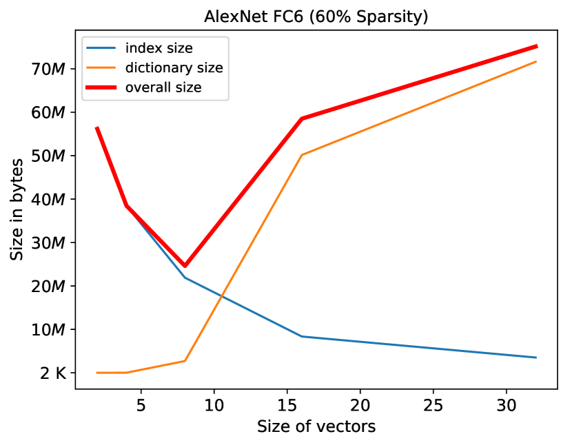
(a) AlexNet FC6

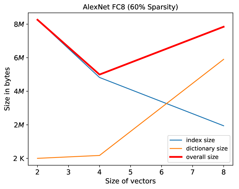
(b) AlexNet FC8

Figure 10. Impact of vector sizes on model compacting. The curves are the lower the better. Compaction ratio goes worse with the vector size increasing. However, the cost introduced by index decreasing. Table 3 shows the best recorded vector sizes.

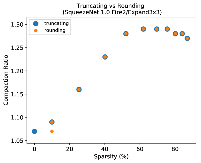
(a) ’squeeze’ layer from SqueezeNet 1.0

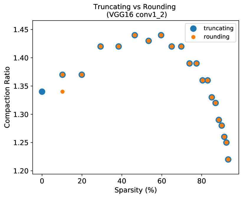
(b) Convolutional layer from VGG16

Figure 11. Comparison between the compaction ratio when using truncation and rounding

Finally, we investigated the effect of either quantizing the weights by rounding to the nearest representable value or by simple truncation. The results show that both approaches provide almost identical levels of block sharing. Given that rounding to the nearest value gives a slightly higher accuracy, this is the method that should be used.

6. Vector Sharing vs Element Sharing

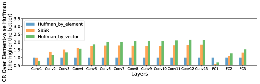
(a) Normalized size of memory consumption on VGG16

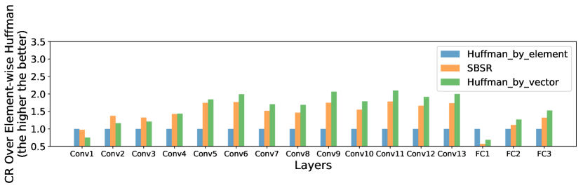
(b) Normalized size of memory consumption on VGG16, but 10-20% Sparser than 12(a)

Figure 12. Comparison between element-wise and vector-wise Huffman coding on VGG-16

For compression of the weight data after pruning, Huffman coding is a widely advocated method. However, existing work focuses on element-wise encoding, e.g. Deep Compression (Han et al., 2015a) which replaces every weight with a variable-length code to reduce the size of the sparse tensor. Though effective, element-wise Huffman coding works suboptimally in many cases because it ignores repeated patterns of values, leading to missed opportunities for compression.

While SBSR works conceptually like a linked list of blocks, the Huffman coding algorithm encodes symbols by building a binary tree according to their occurrence frequencies. All symbols are leaves of the tree while the path to a given leaf is its Huffman code. Rather than assigning every symbol a fixed length code, Huffman coding introduces a variable-length code which allocates fewer code bits to symbols that occur more often. The overall size of the memory requirement is therefore reduced by the use of shorter codes for higher frequency values.

It is straightforward to see how a block-sparse representation exploits patterns in nonzeroes to increase the efficiency of storage. Each index incurs some overhead, so when indices address blocks of data, rather than single elements, the overhead is amortized by the size of the blocks, at the expense of a slight increase in the number of stored zeroes in partial blocks.

In order to capture repeated patterns of values using Huffman coding, we propose vector-wise Huffman coding, which assigns a code to a vector of values, as opposed to individual matrix elements. To fully understand the advantage of vector-wise coding over element-wise coding, we do a breakdown analysis. We then compare the memory reduction from SBSR, vector-wise Huffman coding and element-wise Huffman coding.

The storage required by element-wise Huffman coding consists of three parts: indices, variable-length codes and the encoding dictionary. The memory requirement is calculated as shown in Equation 3.

(3) $$\small Huff\_Size=H_{Idx}+H_{dict}+\sum_{i=1}^{Size\_of\_Dict}{code\_length_{i}\times freq_{i}}$$

The indices $H_{Idx}$ represent the row and column index of the encoded data in the weight matrix. For element-wise Huffman coding, the value indexed is a single non-zero matrix element, while for vector-wise encoding, the value is a weight vector. $H_{Dict}$ is a lookup table with two columns, with one column listing Huffman codes and the other presenting the original value. It contains the necessary information for decoding the weights.

After replacing each element of the tensor with its Huffman code, the memory required to store the encoded values is the sum of the code size times its frequency. We use the formula $\sum_{i=1}^{Size\_of\_Dict}{code\_length\times freq}$ to denote this.

To compare vector- and element-wise encoding methods, we use element-wise Huffman coding (Han et al., 2015a) as our baseline. We use the Compaction Ratio (CR) on graphs as a metric to evaluate the comparison. The CR is read as the “improvement” in compression versus element-wise Huffman coding (so larger CR represents greater compression).

We calculate CR as shown in Equations 4 and 5.

(4) $$\small CR\_huffman=\frac{Size\_of\_Element\_Wise\_Huffman}{Size\_of\_Vector\_Wise\_Huffman}$$

(5) $$\small CR\_SBSR=\frac{Size\_of\_Element\_Wise\_Huffman}{Size\_of\_SBSR}$$

Figure 12 presents the result of vector-wise over element-wise compaction. Limited by the length requirement of the paper, we only present the experiment carried out on the VGG-16 network. Similar results have been found across other networks in fact. All of the 16 layers, including 13 convolutional layers (Conv) and 3 fully connected (FC) layers, have been examined in our experiment. Besides all layers, the network under two different sparsities is also examined. Though the sparsity varies across layers in practice, on average, each layer in Figure 12(a) is 10-20% sparser than in Figure 12(b).

As presented in Figure 12, in most cases, the vector-wise sharing works better than element-sharing. There are two exceptions, which are the layers Conv1 and FC1 in our experiment. The front layers usually come with low sparsities. In our experiment, the sparsity of the Conv1 is the lowest. Because the length of the vector-based dictionary is much larger than element-based one for a dense matrix, extra code bits and storage space are required accordingly. Therefore, the element-wise Huffman coding works better than the vector-wise implementation. However, as SBSR does not require encoding, it works equally well as the element-wise Huffman. For the FC1 layer, the reason that vector-sharing comes worse than element-sharing is that the vector size is too small. Here we select size 2 for all fully connected layers. The FC1 suffers a poor storage ratio while the other two layers experience enhanced compaction. Once given a larger vector, as we can see from the Figure 13 that enlarges the size to 4 elements, all FC layers with vector-wise sharing are better than element-wise Huffman. In general, vector-wise Huffman coding works better than SBSR which is far better than element-wise Huffman coding.

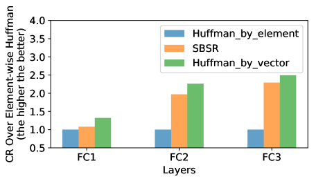
Figure 13. Using a larger vector to the fully connected layers. In this experiment, the size of vector is 4.

To further understand the memory consumption, we break down the equation 2 and 3 to examine the contribution of each component. Figure 14 shows the percentage of memory required by each item in the equations for element-wise Huffman coding, vector-wise Huffman coding, and the SBSR. As we can see in the Figure 14, in most of the cases, space spent on storing index dominates the whole memory usage. However, the memory gap between the index and others are larger for element-wise Huffman Coding, e.g. bars in Figure 14(a), than the vector-sharing methods, e.g. Figure 14(b) and Figure 14(c). Optimising the dominant component can effectively reduce the size of overall memory consumption.

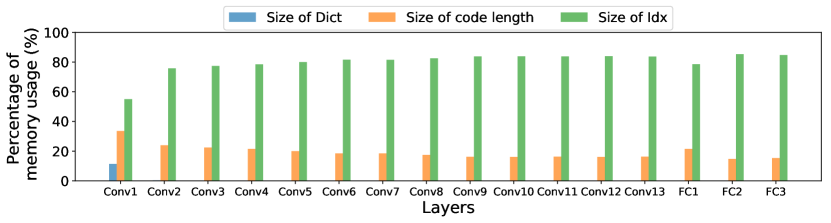
(a) Element-wise Huffman Size Breakdown

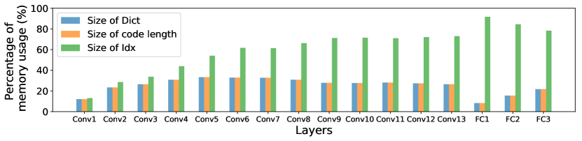
(b) Vector-wise Huffman Size Breakdown

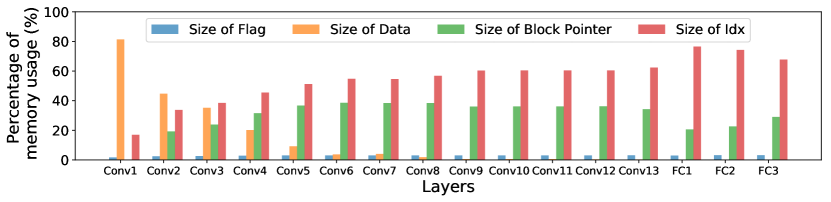
(c) SBSR Size Breakdown

Figure 14. Comparison between the element-wise and vector-wise sharing

6.1. Discussion Between SBSR and Huffman coding

Though both vector-wise Huffman coding and SBSR works better than element-wise sharing, these two methods proposed in this paper have some fundamental difference. As the Huffman coding builds a binary tree on the vectors according to their repeated frequency, its performance complexity is $O(nlogn)$. To the contrary, the SBSR does not require to sort the vector. It can be created by a single scan of the tensor; therefore, its computation complexity is $O(n)$. For extracting the value, both vector-wise Huffman coding and the SBSR has the complexity of $O(1)$. For Huffman coding, the indices are used to get the code first and then decode it by checking the dictionary. For the SBSR, the indices are used to get the block in the SBSR. By checking the flag, we can acquire the value directly or a pointer which leads us to the value.

Apart from the performance complexity, the SBSR are more flexible than the Huffman coding. For each time when the values changed, we have to rebuild the Huffman tree accordingly. However, the SBSR format can handle such issue easily. As it works as a link list, we can insert a new node or simply update the pointer once the vector changed.

In general, there is a compensation between the two implementations we provided in this paper. The vector-wise Huffman coding provides a better compaction ratio, while the SBSR has a higher performance and flexibility.

7. Conclusion

Network pruning and quantization are successful techniques that can efficiently reduce the size of trained CNN models. However, even after pruning and quantization there remains significant redundancy in the form of repeated patterns among the trained parameters. In this paper we propose a novel approach to compacting trained CNNs by exploiting this kind of redundancy. We build upon the existing block-sparse row format for sparse matrices, by sharing a single copy of duplicate blocks. Repeated blocks are replaced by a reference pointing to their first appearance. We evaluated our approach on several well-known CNNs and found that it results in compaction ratios of 1.4$\times$ to 3.1$\times$ in addition to the saving from network pruning and quantization.

We also evaluated element-wise Huffman coding to compress the weight matrices, and implemented an improved block Huffman coding scheme. Both our SBSR approach and block Huffman coding improve compression over element-wise Huffman coding on VGG-16 weight matrices, with an average improvement of $1.53\times$ (SBSR) and $1.67\times$ (block Huffman coding) across all weight tensors in the network.

References

- (1)
- Anwar et al. (2017) Sajid Anwar, Kyuyeon Hwang, and Wonyong Sung. 2017. Structured Pruning of Deep Convolutional Neural Networks. JETC 13, 3 (2017), 32:1–32:18.
- Denil et al. (2013) Misha Denil, Babak Shakibi, Laurent Dinh, Marc’Aurelio Ranzato, and Nando de Freitas. 2013. Predicting Parameters in Deep Learning. In NIPS. 2148–2156.
- Ding et al. (2017) Caiwen Ding, Siyu Liao, Yanzhi Wang, Zhe Li, Ning Liu, Youwei Zhuo, Chao Wang, Xuehai Qian, Yu Bai, Geng Yuan, Xiaolong Ma, Yipeng Zhang, Jian Tang, Qinru Qiu, Xue Lin, and Bo Yuan. 2017. CirCNN: accelerating and compressing deep neural networks using block-circulant weight matrices. In MICRO. ACM, 395–408.
- Engelbrecht (2001) Andries Engelbrecht. 2001. A new pruning heuristic based on variance analysis of sensitivity information. 12 (12 2001), 1386 – 1399.
- Franklin (2017) Dustin Franklin. 2017. NVIDIA Jetson TX2 Delivers Twice the Intelligence to the Edge. Retrieved from https://devblogs.nvidia.com/jetson-tx2-delivers-twice-intelligence-edge/
- González and Woods (2008) Rafael C. González and Richard E. Woods. 2008. Digital image processing, 3rd Edition. Pearson Education.
- Guo et al. (2016) Yiwen Guo, Anbang Yao, and Yurong Chen. 2016. Dynamic Network Surgery for Efficient DNNs. In NIPS. 1379–1387.
- Gysel et al. (2016) Philipp Gysel, Mohammad Motamedi, and Soheil Ghiasi. 2016. Hardware-oriented Approximation of Convolutional Neural Networks. CoRR abs/1604.03168 (2016).
- Han et al. (2015a) Song Han, Huizi Mao, and William J. Dally. 2015a. Deep Compression: Compressing Deep Neural Network with Pruning, Trained Quantization and Huffman Coding. CoRR abs/1510.00149 (2015).
- Han et al. (2015b) Song Han, Jeff Pool, John Tran, and William J. Dally. 2015b. Learning both Weights and Connections for Efficient Neural Network. In NIPS. 1135–1143.
- Hassibi and Stork (1992) Babak Hassibi and David G. Stork. 1992. Second Order Derivatives for Network Pruning: Optimal Brain Surgeon. In NIPS. Morgan Kaufmann, 164–171.
- He et al. (2017) Yihui He, Xiangyu Zhang, and Jian Sun. 2017. Channel Pruning for Accelerating Very Deep Neural Networks. In ICCV. IEEE Computer Society, 1398–1406.
- Hu et al. (2016) Hengyuan Hu, Rui Peng, Yu-Wing Tai, and Chi-Keung Tang. 2016. Network Trimming: A Data-Driven Neuron Pruning Approach towards Efficient Deep Architectures. CoRR abs/1607.03250 (2016).
- Iandola et al. (2016) Forrest N. Iandola, Matthew W. Moskewicz, Khalid Ashraf, Song Han, William J. Dally, and Kurt Keutzer. 2016. SqueezeNet: AlexNet-level accuracy with 50x fewer parameters and <1MB model size. CoRR abs/1602.07360 (2016).
- Judd et al. (2017) Patrick Judd, Jorge Albericio, and Andreas Moshovos. 2017. Stripes: Bit-Serial Deep Neural Network Computing. Computer Architecture Letters 16, 1 (2017), 80–83.
- Kepner et al. (2017) Jeremy Kepner, Manoj Kumar, José E. Moreira, Pratap Pattnaik, Mauricio J. Serrano, and Henry M. Tufo. 2017. Enabling Massive Deep Neural Networks with the GraphBLAS. CoRR abs/1708.02937 (2017).
- LeCun et al. (1989) Yann LeCun, John S. Denker, and Sara A. Solla. 1989. Optimal Brain Damage. In NIPS. Morgan Kaufmann, 598–605.
- Li et al. (2016) Hao Li, Asim Kadav, Igor Durdanovic, Hanan Samet, and Hans Peter Graf. 2016. Pruning Filters for Efficient ConvNets. CoRR abs/1608.08710 (2016).
- Lin et al. (2017) Ji Lin, Yongming Rao, Jiwen Lu, and Jie Zhou. 2017. Runtime Neural Pruning. In NIPS. 2178–2188.
- Luo et al. (2017) Jian-Hao Luo, Jianxin Wu, and Weiyao Lin. 2017. ThiNet: A Filter Level Pruning Method for Deep Neural Network Compression. In ICCV. IEEE Computer Society, 5068–5076.
- Mao et al. (2017) Huizi Mao, Song Han, Jeff Pool, Wenshuo Li, Xingyu Liu, Yu Wang, and William J. Dally. 2017. Exploring the Granularity of Sparsity in Convolutional Neural Networks. In CVPR Workshops. IEEE Computer Society, 1927–1934.
- Moons and Verhelst (2016) Bert Moons and Marian Verhelst. 2016. A 0.3-2.6 TOPS/W precision-scalable processor for real-time large-scale ConvNets. In VLSI Circuits. IEEE, 1–2.
- Saad (2003) Yousef Saad. 2003. Iterative methods for sparse linear systems. SIAM.
- Sze et al. (2017) Vivienne Sze, Yu-Hsin Chen, Tien-Ju Yang, and Joel S. Emer. 2017. Efficient Processing of Deep Neural Networks: A Tutorial and Survey. Proc. IEEE 105, 12 (2017), 2295–2329.
- Vanhoucke et al. (2011) Vincent Vanhoucke, Andrew Senior, and Mark Z. Mao. 2011. Improving the speed of neural networks on CPUs. In Deep Learning and Unsupervised Feature Learning Workshop, NIPS 2011.
- Williams et al. (2007) Samuel Williams, Leonid Oliker, Richard W. Vuduc, John Shalf, Katherine A. Yelick, and James Demmel. 2007. Optimization of sparse matrix-vector multiplication on emerging multicore platforms. In SC. ACM Press, 38.
- Yang et al. (2017b) Tien-Ju Yang, Yu-Hsin Chen, Joel S. Emer, and Vivienne Sze. 2017b. A method to estimate the energy consumption of deep neural networks. In ACSSC. IEEE, 1916–1920.
- Yang et al. (2017a) Tien-Ju Yang, Yu-Hsin Chen, and Vivienne Sze. 2017a. Designing Energy-Efficient Convolutional Neural Networks Using Energy-Aware Pruning. In CVPR. IEEE Computer Society, 6071–6079.
- Yu et al. (2017) Jiecao Yu, Andrew Lukefahr, David J. Palframan, Ganesh S. Dasika, Reetuparna Das, and Scott A. Mahlke. 2017. Scalpel: Customizing DNN Pruning to the Underlying Hardware Parallelism. In ISCA. ACM, 548–560.