How to Count Triangles, without Seeing the Whole Graph

Abstract.

Triangle counting is a fundamental problem in the analysis of large graphs. There is a rich body of work on this problem, in varying streaming and distributed models, yet all these algorithms require reading the whole input graph. In many scenarios, we do not have access to the whole graph, and can only sample a small portion of the graph (typically through crawling). In such a setting, how can we accurately estimate the triangle count of the graph?

We formally study triangle counting in the random walk access model introduced by Dasgupta et al (WWW ’14) and Chierichetti et al (WWW ’16). We have access to an arbitrary seed vertex of the graph, and can only perform random walks. This model is restrictive in access and captures the challenges of collecting real-world graphs. Even sampling a uniform random vertex is a hard task in this model.

Despite these challenges, we design a provable and practical algorithm, TETRIS, for triangle counting in this model. TETRIS is the first provably sublinear algorithm (for most natural parameter settings) that approximates the triangle count in the random walk model, for graphs with low mixing time. Our result builds on recent advances in the theory of sublinear algorithms. The final sample built by TETRIS is a careful mix of random walks and degree-biased sampling of neighborhoods. Empirically, TETRIS accurately counts triangles on a variety of large graphs, getting estimates within 5% relative error by looking at 3% of the number of edges.

1. Introduction

Triangle counting is a fundamental problem in the domain of network science. The triangle count (and variants thereof) appears in many classic parameters in social network analysis such as the clustering coefficient (Newman, 2003), transitivity ratio (Wasserman and Faust, 1994), local clustering coefficients (Watts and Strogatz, 1998). Some example applications of this problem are motifs discovery in complex biological networks (Milo et al., 2002), modeling large graphs (Seshadhri et al., 2012; III et al., 2012, 2014), indexing graph databases (Khan et al., 2011), and spam and fraud detection cyber security (Becchetti et al., 2008). Refer to the tutorial (Seshadhri and Tirthapura, 2019) for more applications.

Given full access to the input graph $G$, we can exactly count the number of triangles in $O(m^{3/2})$ time (Itai and Rodeh, 1978), where $m$ is the number of edges in $G$. Exploiting degree based ordering, the runtime can be improved to $O(m\alpha)$ (Chiba and Nishizeki, 1985), where $\alpha$ is the maximum core number (degeneracy) of $G$. In various streaming and distributed models, the triangle counting problem has a rich theory (Bar-Yossef et al., 2002; Jowhari and Ghodsi, 2005; Buriol et al., 2006; Cohen, 2009; Suri and Vassilvitskii, 2011; Kolda et al., 2014; McGregor et al., 2016; Bera and Chakrabarti, 2017; Bera and Seshadhri, 2020), and widely used practical algorithm (Becchetti et al., 2008; Jha et al., 2013; Pavan et al., 2013; Tangwongsan et al., 2013; Ahmed et al., 2014a; Chen et al., 2016; Stefani et al., 2017; Türkoglu and Turk, 2017; Turk and Turkoglu, 2019).

Yet the majority of these algorithms, at some point, read the entire graph. (The only exceptions are the MCMC based algorithms (Rahman and Hasan, 2014; Chen et al., 2016), but they require global parameters for appropriate normalization. We explain in detail later.) In many practical scenarios, the entire graph is not known. Even basic graph parameters such as the total number of vertices and the number of edges are unknown. Typically, a sample of the graph is obtained by crawling the graph, from which properties of the true graph must be inferred. In common network analysis settings, practitioners crawl some portion of the (say) coauthor, web, Facebook, Twitter, etc. network. They perform experiments on this sample, in the hope of inferring the “true” properties of the original graph. This sampled graph may be an order of magnitude smaller than the true graph.

There is a rich literature on graph sampling, but arguably, Dasgupta et al. (Dasgupta et al., 2014) gave the first formalization of this sampling through the random walk access model. In this model, we have access to some arbitrary seed vertex. We can discover portions of the graph by performing random walks/crawls starting at this vertex. At any vertex, we can retrieve two basic pieces of information — its degree and a uniform random neighbor. Rudimentary graph mining tasks such as sampling a uniform random node is non-trivial in this model. Dasgupta et al. (Dasgupta et al., 2014) showed how to find the average degree of the graph in this model. Chierichetti et al. (Chierichetti et al., 2016) gave an elegant algorithm for sampling a uniform random vertex. Can we estimate more involved graph properties efficiently in this model? This leads to the main research question behind this work.

How can we accurately estimate the triangle count of the graph by observing only a tiny fraction of it in the random walk access model?

There is a rich literature of sampling-based triangle counting algorithms (Schank and Wagner, 2005; Buriol et al., 2006; Tsourakakis et al., 2009; Jha et al., 2013; Pavan et al., 2013; Seshadhri et al., 2014; Ahmed et al., 2014a; Türkoglu and Turk, 2017; Turk and Turkoglu, 2019). However, all of these algorithms heavily relies on uniform random edge samples or uniform random vertex samples. Such samples are computationally expensive to generate in the random walk access model. To make matters worse, we do not know the number of vertices or edges in the graph. Most sampling algorithms require these quantities to compute their final estimate.

1.1. Problem description

In this paper, we study the triangle estimation problem. Given limited access to an input graph $G=(V,E)$, our goal is to design an $(\varepsilon,\delta)$-estimator for the triangle count.

Definition 1.1.

Let $\varepsilon,\delta\in[0,1]$ be two parameters and $T$ denote the triangle counting. A randomized algorithm is an $(\varepsilon,\delta)$-estimator for the triangle counting problem if: the algorithm outputs estimate $\overline{T}$ such that with probability (over the randomness of the algorithm) at least $1-\delta$, $(1-\varepsilon)T\leqslant\overline{T}\leqslant(1+\varepsilon)T$. (We stress that there is no stochastic assumption on the input itself.)

The random walk access model: In designing an algorithm, we aim to minimize access to the input graph. To formalize, we required a query model and follow models given in Dasgupta et al. (Dasgupta et al., 2014) and Chierichetti et al. (Chierichetti et al., 2016).

The algorithm initially has access to a single, arbitrary seed vertex $s$. The algorithm can make three types of queries:

• Random Neighbor Query: Given a vertex $v\in V$, acquire a uniform random neighbor of $v$.

• Degree Query: Given a vertex $v\in V$, acquire the degree of $v$.

• Edge Query: Given two vertices $u,v\in V$, acquire whether the edge $\{u,v\}$ is present in the graph.

Starting from $s$, the algorithm makes queries to discover more vertices, makes queries from these newly discovered vertices to see more of the graph, so on and so forth. An algorithm in this model does not have free access to the set of vertices. It can only make degree queries and edge queries on the vertices that have been observed during the random walk. We emphasize that the random walk does not start from an uniform random vertex; the seed vertex is arbitrary. In fact, generating a uniform vertex in this model is a non-trivial task and explicitly studied by Chierichetti et al. (Chierichetti et al., 2016) We note a technical difference between the above model and those studied in (Dasgupta et al., 2014; Chierichetti et al., 2016). Some of these results assume all neighbors can be obtained with a single query, while we assume a query gives a random neighbor. As a first step towards sublinear algorithms, we feel that the latter is more appropriate to understand how much of graph needs to be sampled to estimate the triangle counting. But it would be equally interesting to study different query models.

We do not assume prior knowledge on the number of vertices or edges in the graph. This is consistent with many practical scenarios, such as API based online networks, where estimating $|E|$ itself is a challenging task. The model as defined is extremely restrictive, making it challenging to design provably accurate algorithms in this model.

On uniform vertex/edge samples: There is a large body of theoretical and practical work efficient on efficient triangle counting assuming uniform random vertex or edge samples (the latter is often simulated by streaming algorithms) (Bar-Yossef et al., 2002; Jowhari and Ghodsi, 2005; Schank and Wagner, 2005; Buriol et al., 2006; Tsourakakis et al., 2009; Kolountzakis et al., 2012; Wu et al., 2016; McGregor et al., 2016; Bera and Chakrabarti, 2017; Bera and Seshadhri, 2020). However, when uniform random vertex or edge samples are not available, as is the case in our model, the existing literature is surprisingly quiet.

Complexity measure: While designing an $(\varepsilon,\delta)$-estimator in the random walk model, our goal is to minimize the number of queries made. We do not deal with running time (though our final algorithm is also time-efficient). For empirical results, we express queries as a fraction of $m$, the total number of edges. In mathematical statements, we sometimes use the $\widetilde{O}$ notation to hide dependencies on $\varepsilon,\delta,\log n$.

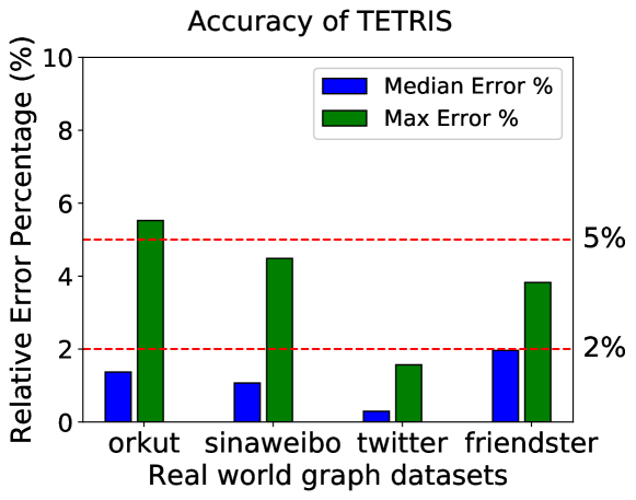
Figure 1. Accuracy of TETRIS on real datasets: soc-orkut (3M vertices, 213M edges), soc-siaweibo (59M vertices, 523M edges), soc-twitter(42M vertices, 2.4B edges), soc-friendster(66M vertices, 3.6B edges). We run TETRIS with exact same set of parameters for all the datasets and observes only 3% of the edges. We repeat the experiments for 100 times. Remarkably for 100 independent runs, TETRIS achieves worst case relative error of about 5% (the green bar in the plot) and median relative error of 2% (the blue bar in the plot).

1.2. Our contributions

In this work, we present a novel algorithm, Triangle Estimation Through Random Incidence Sampling, or TETRIS, that solves the triangle counting problem efficiently in the random walk access model. TETRIS provably outputs an $(\varepsilon,\delta)$-estimator for the triangle counting problem. Under common assumptions on the input graph $G$, TETRIS is provably sublinear. In practice, TETRIS is highly accurate and robust. Applying to real datasets, we demonstrate that, it only needs to observe a tiny fraction of the graph to make an accurate estimation of the triangle count (see  Figure 1).

First provably sublinear triangle counting algorithm in the random walk access model.  Our algorithm TETRIS builds on recent theoretical results in sublinear algorithms for clique counting (Eden et al., 2015, 2020). Our central idea is to sample edges proportional to a somewhat non-intuitive quantity: the degree of the lower degree endpoint of the edge. In general, such weighted sampling is impossible to achieve in the random walk access model. However, borrowing techniques from Eden et al. (Eden et al., 2020), we approximately simulate such a sample in this model. By a careful analysis of various components, we prove that TETRIS is an $(\varepsilon,\delta)$-estimator.

Accurate and robust empirical behavior.  We run TETRIS on a collection of massive datasets, each with more than 100 million edges. For all instances, TETRIS achieves less than 3% median relative error while observing less than 3% of the graph. Results are shown in Figure 1. Even over a hundred runs (on each dataset), TETRIS has a maximum error of at most 5%. We also empirically demonstrate the robustness of our algorithm against various choices for the seed vertex.

Comparison with existing sampling based methods.  While the vast majority of triangle counting algorithm read the whole graph, the MCMC algorithms of Rahman et al. (Rahman and Hasan, 2014) and Chen et al. (Chen et al., 2016) can be directly adapted to the random walk access model. We also note that the sparsification algorithm of Tsourakakis et al. (Tsourakakis et al., 2009) and the sampling method of Wu et al. (Wu et al., 2016) can be implemented (with some changes) in the random walk model. We perform head to head comparisons of TETRIS with these algorithms. We observe that TETRIS is the only algorithm that consistently has a low error in all instances. The Subgraph Random walk of Chen et al. (Chen et al., 2016) has a reasonable performance across all instances, though its error is typically double of TETRIS. All other algorithms have an extremely high error on some input. These findings are consistent with our theoretical analysis of TETRIS, which proves sublinear query complexity (under certain conditions on graph parameters).

1.3. Main Theorem

Our main theoretical contribution is to prove that Triangle Estimation Through Random Incidence Sampling, or TETRIS is an $(\varepsilon,\delta)$-estimator for the triangle counting problem. Let $G$ be the input graph with $m$ edges and maximum core number (degeneracy) $\alpha$. We use $t_{e}$ to denote the number of triangles incident on an edge $e$. Define the maximum value of $t_{e}$ as $t_{\operatorname{max}}:=\max_{e\in E}t_{e}$. Assume the total number of triangles is $T$. We denote the mixing time of the input graph as $\operatorname{\ell_{mix}}$.

Theorem 1.2.

Let $\varepsilon,\delta\in[0,1]$ be some parameters and $G$ be an arbitrary input graph. Then TETRIS produces an $(\varepsilon,\delta)$-estimate for the triangle count in the random walk access model. Moreover, the number of queries made by TETRIS is at most

$$O\left(\log\left(\frac{1}{\delta}\right)\frac{\log n}{\varepsilon^{2}}\left(\frac{m\operatorname{\ell_{mix}}t_{\operatorname{max}}}{T}+\frac{m\alpha}{T}+\sqrt{m}\operatorname{\ell_{mix}}\right)\right)\,.$$

The runtime and the space requirement of TETRIS is bounded by the same quantity as well.

The quantities $\alpha$ and $\operatorname{\ell_{mix}}$ are considered small in social networks. Moreover, $t_{\operatorname{max}}$ is much smaller than the total triangle count $T$. Thus, the bound above is strictly sublinear for social networks. Moreover, it is known that lower bound of $\operatorname{\ell_{mix}}$ is necessary even for the simpler problem of sampling vertices (Chierichetti and Haddadan, 2018).

1.4. Main Ideas and Challenges

Sampling based triangle counting algorithms typically work as follows. One associates some quantity (like the triangle count of an edge) to each edge, and estimates the sum of this quantity by randomly sampling edges. If uniform random edges are present, then one can use standard scaling to estimate the sum ((Tsourakakis et al., 2009; Kolountzakis et al., 2012; Wu et al., 2016)). Other methods set up a highly non-uniform distribution, typically biasing more heavily to higher degree vertices, in the hope of catching triangles with fewer samples (the classic method being wedge sampling (Schank and Wagner, 2005; Seshadhri et al., 2014; Rahman and Hasan, 2014; Türkoglu and Turk, 2017)). This is more efficient in terms of samples, but requires more complex sampling and needs non-trivial normalization factors, such as total wedge counts. All of these techniques face problems in the random walk access model. Even if the mixing time $\operatorname{\ell_{mix}}$ is low, one needs $k\operatorname{\ell_{mix}}$ queries to get $k$ truly independent uniform edges. And it could potentially require even more samples to get non-uniform wedge based distributions. Indeed, our experiments show that this overhead leads to inefficient algorithms in the random walk access model.

To get around this problem, we use the key idea of ordering vertices by degree, a common method in triangle counting. Inspired by a very recent sublinear clique counting algorithms of Eden et al. (Eden et al., 2020), we wish to sample edges proportional to the degree of the smaller degree endpoint. Such ideas have been used to speed up wedge sampling (Türkoglu and Turk, 2017; Turk and Turkoglu, 2019). Such a sampling biases away from extremely high degree vertices, which is beneficial in the random walk model.

But how to sample according to this (strange) distribution? Our algorithm is rather naive: simply take a long random walk, and just perform this sampling among the edges of the random walk. Rather surprisingly, this method provably works. The proof requires a number of ideas introduced in (Eden et al., 2020). The latter result requires access to uniform random vertices, but we are able to adapt the proof strategy to the random walk model.

The final algorithm is a direct implementation of the above ideas, though there is some technicality about the unique assignment of triangles to edges. The proof, on the other hand, is quite non-trivial and has many moving parts. We need to show that sampling according to the biased distribution among the edges of the random walk has similar statistical properties to sampling from all edges. This requires careful use of concentration bounds to show that various statistics of the entire set of edges are approximately preserved in the set of random walk edges. Remarkably, the implementation follows the theoretical algorithm exactly. We require no extra heuristics to make the algorithm practical.

We mention some benefits of our approach, in the context of practical sublinear algorithms. We do not need non-trivial scaling factors, like total wedge counts (required for any wedge sampling approach). Also, a number of practical MCMC methods perform random walks on “higher order” Markov Chains where states are small subgraphs of $G$. Any theoretical analysis requires mixing time bounds on these Markov Chains, and it is not clear how to relate these bounds to the properties of $G$. Our theoretical analysis relies only on the mixing time of $G$, and thus leads to a cleaner main theorem. Moreover, a linear dependence of the mixing time is likely necessary, as shown by recent lower bounds (Chierichetti and Haddadan, 2018).

2. Related Work

There is an immense body of literature on the triangle counting problem, and we only focus on work that is directly relevant. For a detailed list of citations, we refer the reader to the tutorial (Seshadhri and Tirthapura, 2019).

There are a number of exact triangle counting algorithms, often based on the classic work of Chiba-Nishizeki (Chiba and Nishizeki, 1985). Many of these algorithms have been improved by using clever heuristics, parallelism, or implementations that reduce disk I/O (Schank and Wagner, 2005; Hu et al., 2014; Green et al., 2014; Azad et al., 2015; Kim et al., 2016).

Approximate triangle counting algorithms are significantly faster and more widely studied in both theory and practice. Many techniques have been explored to solve this problem efficiently in the streaming model, the map-reduce model, and the general static model (or RAM model). There are plethora of practical streaming algorithms (Becchetti et al., 2008; Jha et al., 2013; Pavan et al., 2013; Tangwongsan et al., 2013; Ahmed et al., 2014a; Jha et al., 2015; Stefani et al., 2017), MapReduce algorithms (Cohen, 2009; Suri and Vassilvitskii, 2011; Kolda et al., 2014), and other distributed models (Kolountzakis et al., 2012; Arifuzzaman et al., 2013) as well. Even in the static settings, sampling based approaches have been proven quite efficient  (Tsourakakis et al., 2009; Seshadhri et al., 2014; Etemadi et al., 2016; Türkoglu and Turk, 2017; Turk and Turkoglu, 2019) for this problem.

All of these algorithms read the entire input, with the notable exception of MCMC based algorithms (Rahman and Hasan, 2014; Chen et al., 2016). These algorithms perform a random walk in a “higher” order graph, that can be locally constructed by looking at the neighborhoods of a vertex. We can implement these algorithms in the random walk access model, and indeed, consider these to be the state-of-the-art triangle counting algorithms for this model. We note that these results are not provably sublinear (nor do they claim to be so). Nonetheless, we find they perform quite well in terms of making few queries to get accurate estimates for the triangle count. Notably, the Subgraph Random Walk algorithm of (Chen et al., 2016) is the only other algorithm that gets reasonable performance in all instances, and the VertexMCMC algorithm of (Rahman and Hasan, 2014) is the only algorithm that ever outperforms TETRIS (though in other instances, it does not seem to converge).

We note that the Doulion algorithm of Tsourakakis et al. (Tsourakakis et al., 2009) and the sampling method of Wu et al. (Wu et al., 2016) can also be implemented in the random walk access model. Essentially, we can replace their set of uniform random edges with the set of edges produced by a random walk (with the hope that after the mixing time, the set “behaves” uniform). We observe that these methods do not perform too well.

From a purely theoretical standpoint, there have been recent sublinear algorithms for triangle counting by Eden et al. (Eden et al., 2015, 2020). These algorithms require access to uniform random samples and cannot be implemented directly in the random walk model. Nonetheless, the techniques from these results are highly relevant for TETRIS. In particular, we borrow the two-phase sampling idea from (Eden et al., 2015, 2017) to simulate the generation of edge samples according to edge based degree distribution.

The random walk access model is formalized by Dasgupta et al. (Dasgupta et al., 2014) in the context of the average degree estimation problem. Prior to that, there have been several works on estimating basic statistics of a massive network through crawling. Katzir et al. (Katzir et al., 2011), Hardiman et al. (Hardiman et al., 2009), and Hardiman and Katzir (Katzir and Hardiman, 2015) used collisions to estimate graph sizes and clustering coefficients of individual vertices. Cooper et al. (Cooper et al., 2014) used random walks for estimating various network parameters, however, their sample complexity is still is at least that of collision based approaches. Chierichetti et al. (Chierichetti et al., 2016) studied the problem of uniformly sampling a node in the random walk access model. Many triangle counting estimators are built on uniform random node samples. However, using the uniform node sampler of Chierichetti et al. (Chierichetti et al., 2016) leads to an expensive triangle estimator, because of the overhead of generating vertex samples.

There are quite a few sampling methods based on random crawling: forest-fire (Leskovec and Faloutsos, 2006), snowball sampling (Maiya and Berger-Wolf, 2011), and expansion sampling (Leskovec and Faloutsos, 2006). However, they do not lead to unbiased estimators for the triangle counting problem. It is not clear whether such sampling methods can generate provably accurate estimator for this problem. For a more detailed survey of various sampling methods for graph parameter estimation, we refer to the works of Leskovec and Faloutsos (Leskovec and Faloutsos, 2006), Maiya and Berger-Wolf (Maiya and Berger-Wolf, 2011), and Ahmed, Neville, and Kompella (Ahmed et al., 2014b).

3. Preliminaries

In this paper, graphs are undirected and unweighted. We denote the input graph by $G=(V,E)$, and put $|V|=n$ and $|E|=m$. We denote the number of triangles in the input graph by $T$. For an integer $k$, we denote the set $\{1,2,,\ldots k\}$ by $[k]$. All the logarithms are base $2$.

For a vertex $v\in V$, we denote its neighborhood as $N(v):=\{u:\{u,v\}\in E\}$, and degree as $d(v):=|N(v)|$. For an edge $e=\{u,v\}\in E$, we define degree of $e$ as the minimum degree of its endpoint: $d(e):=\min\{d(u),d(v)\}$. Similarly, we define the neighborhood of $e$: $N(e)=N(u)$ if $d(u)<d(v)$, $N(e)=N(v)$ otherwise.

We consider a degree based ordering of the vertices $\prec_{\deg}$: for two vertices $u,v\in V$, $u\prec_{\deg}v$ iff $d(u)<d(v)$ or $d(u)=d(v)$ and $u$ precedes $v$ according some fixed ordering, say lexicographic ordering. Every triangle is uniquely assigned to an edge as follows. For a triangle $\{v_{1},v_{2},v_{3}\}$ such that $v_{1}\prec_{\deg}v_{2}\prec_{\deg}v_{3}$, we assign it to the edge $(v_{1},v_{2})$. We denote the number of triangles associated with an edge $e$ by $t_{e}$. Clearly, $\sum_{e\in E}t_{e}=T$. We denote by $t_{\max}$ the maximum number of triangles associated with any edge: $t_{\max}=\max_{e\in E}t_{e}$.

We extend the notion of $d_{e}$ and $t_{e}$ to a collection of edges $R$ naturally: $d_{R}=\sum_{e\in R}d_{e}$ and $t_{R}=\sum_{e\in R}t_{e}$. Note that if $R$ is a multi-set, then we treat every occurrences of an edge $e$ as a distinct member of $R$, and the quantities $d_{R}$ and $t_{R}$ reflect these.

We denote the degeneracy (or the maximum core number) of the input graph by $\alpha$. Degeneracy, or the maximum core number, is the smallest integer $k$, such that for every subgraph in the input graph, there is a vertex of degree at most $k$. Chiba and Nishizeki proved the following connection between $\alpha$ and $d_{E}$.

Lemma 3.1 (Chiba and Nishizeki (Chiba and Nishizeki, 1985)).

$d_{E}=\sum_{e\in E}d_{e}=O(m\alpha$).

We revisit a few basic notions about the random walk on a connected, undirected, non-bipartite graph. For every graph, $\pi(v)=\frac{d(v)}{2m}$ is the stationary distribution. We denote the mixing time of the input graph by $\operatorname{\ell_{mix}}$.

We use the following concentration bounds for analyzing our algorithms. In general, we use the shorthand $A\in(1\pm\varepsilon)B$ for $A\in[(1-\varepsilon)B,(1+\varepsilon)B]$.

Theorem 3.2.

• Let $X_{1},X_{2},\ldots,X_{r}$ be mutually independent indicator random variables with expectation $\mu$. Then, for every $\varepsilon$ with $0<\varepsilon<1$, $\Pr\left[\sum_{i=1}^{r}X_{i}/r\notin(1\pm\varepsilon)\mu\right]\leqslant 2\exp\left(-\varepsilon^{2}r\mu/3\right)$.

• Let $X$ be a random variable with expectation $\mu$ and variance $\hbox{\bf Var}[X]$. Then, for every $\varepsilon>0$, $\Pr\left[X\notin(1\pm\varepsilon)\mu\right]\leqslant\frac{\hbox{\bf Var}[X]}{\varepsilon^{2}\mu^{2}}$.

4. The Main Result and TETRIS

We begin with the description of our triangle counting algorithm, TETRIS ( Algorithm 1).

It takes three input parameters: the length of the random walk $r$, the number of subsamples (explained below) $\ell$, and an estimate $\widehat{\operatorname{\ell_{mix}}}$ of the mixing time. TETRIS starts with an arbitrary vertex of the graph provided by the model. Then it performs a random walk of length $r$ and collects the edges in a ordered multi-set $R$. For each edge $e=\{u,v\}\in R$, it computes the degree $d_{e}$. Recall the definition of degree of an edge: $d_{e}=\min\{d_{u},d_{v}\}$. Then, TETRIS samples $\ell$ edges from $R$, where edge $e$ is sampled with probability proportional to $d_{e}$.

For an edge $e$ sampled in the above step, TETRIS samples a uniform random neighbor $w$ from $N(e)$; recall $N(e)$ denote the neighbors of the lower degree end point. Finally, using edge queries, TETRIS checks whether a triangle is formed by $\{e,w\}$. If it forms a triangle, TETRIS checks if the triangle is uniquely assigned to the edge $e$ by querying the degrees of the constituent vertices (see Section 3 for the assignment rule).

To compute the final estimate for triangles, TETRIS requires an estimate for the number of edges. To accomplish this task, we design a collision based edge estimator in Algorithm 2, based on a result of Ron and Tsur (Ron and Tsur, 2016).

Algorithm 1 TETRIS— Triangle Counting Estimator

1:procedure TETRIS(integer $r$, integer $\ell$, integer $\widehat{\operatorname{\ell_{mix}}}$)

2:     Let $s$ be some arbitrary vertex provided by the model.

3:     Let $R$ be the multiset of edges on a $r$-length random walk from $s$.

4:     for $i=1$ to $\ell$ do

5:         Sample an edge $e\in R$ independently with prob. $d_{e}/d_{R}$.

6:         Query a uniform random neighbor $w$ from $N(e)$.

7:         Using edge query, check if $\{e,w\}$ forms a triangle.

8:         If $\{e,w\}$ forms a triangle $\tau$: query for degrees of all vertices in $\tau$ and determine if $\tau$ is associated to $e$.

9:         If $\tau$ is associated to $e$, set $Y_{i}=1$; else set $Y_{i}=0$.      

10:     Set $Y=\frac{1}{\ell}\sum_{i=1}^{\ell}Y_{i}$.

11:     Let $\overline{m}$ = EdgeCountEstimator$~{}(R,\widehat{\operatorname{\ell_{mix}}})$

12:     Set $X=\frac{\overline{m}}{r}\cdot d_{R}\cdot Y$.

13:     return $X$.

Algorithm 2 Edge Count Estimator

1:procedure EdgeCountEstimator(edge set $R$, integer $\widehat{\operatorname{\ell_{mix}}}$)

2:     for $i=1$ to $\widehat{\operatorname{\ell_{mix}}}$ do

3:         Let $R_{i}=(e_{i},e_{i+\widehat{\operatorname{\ell_{mix}}}},e_{i+2\widehat{\operatorname{\ell_{mix}}}},\ldots)$.

4:         Set $c_{i}=$number of pairwise collision in $R_{i}$.

5:         Set $Y_{i}=\binom{|R_{i}|}{2}/c_{i}$.      

6:     Set $Y=\frac{1}{\widehat{\operatorname{\ell_{mix}}}}\sum_{i}Y_{i}$.

7:     return $Y$.

We state the guarantees of EdgeCountEstimator. It is a direct consequence of results of Ron and Tsur (Ron and Tsur, 2016), and we defer the formal proof to the Appendix A.

Theorem 4.1.

Let $\varepsilon>0$ be some constant, $\widehat{\operatorname{\ell_{mix}}}\geqslant\operatorname{\ell_{mix}}$, and $|R|\geqslant\frac{\log n}{\varepsilon^{2}}\cdot\operatorname{\ell_{mix}}\cdot\sqrt{m}$. Then, EdgeCountEstimator outputs $\overline{m}\in(1\pm\varepsilon)m$ with probability at least $1-o(1/n)$.

4.1. Theoretical Analysis of TETRIS

We provide a theoretical analysis of TETRIS and prove  Theorem 1.2. We first show that if the collection of edges $R$ exhibits some “nice” properties, then we have an accurate estimator. Then we prove that the collection of edges $R$ produced by the random walk has these desired properties. Our goal is to prove that the output of TETRIS, $X$, is an $(\varepsilon,\delta)$-estimator for the triangle counts. For ease of exposition, in setting parameter values of $r$ and $\ell$, we hide the dependency on the error probability $\delta$. A precise calculation would set the dependency to be $\log(1/\delta)$, as standard in the literature.

We first show that the random variable $Y$ ( 10) roughly captures the ratio $T/d_{E}$. To show this, we first fix an arbitrary collection of edges $R$, and simulate TETRIS on it. We show that, in expectation, $Y$ is going to $t_{R}/d_{R}$. For the sake of clear presentation, we denote the value of the random variable $Y$, when run with the edge collection $R$, to be $Y_{R}$. Note that, $Y_{R}$ is a random variable nevertheless; the source of the randomness lies in the $\ell$ many random experiments that TETRIS does in each iteration of the for loop at  4 of  Algorithm 1

Lemma 4.2.

Let $R$ be a fixed collection of edges, and $Y_{R}$ denote the value of the random variable $Y$ on the fixed set $R$ ( 10 of  Algorithm 1). Then,

1. $\hbox{\bf E}[Y_{R}]=\frac{t_{R}}{d_{R}}$,

2. $\Pr\left[~{}|Y_{R}-\hbox{\bf E}[Y_{R}]|\geqslant\varepsilon\hbox{\bf E}[Y_{R}]~{}\right]\leqslant\exp\left(-\ell\cdot\frac{\varepsilon^{2}}{3}\cdot\frac{t_{R}}{d_{R}}\right)$.

Proof.

We first prove the expectation statement. Let $e_{i}$ be the random variable that denotes the edge sampled in the $i$-th iteration of the for loop ( 4). Consider the random variable $Y_{i}$. We have

$$\Pr[Y_{i}=1] =\sum_{e\in R}\Pr[e_{i}=e]\Pr[Y_{i}=1|e_{i}=e]\,,$$

$$=\sum_{e\in R}\frac{d_{e}}{d_{R}}\Pr[Y_{i}=1|e_{i}=e]=\sum_{e\in R}\frac{t_{e}}{d_{R}}=\frac{t_{R}}{d_{R}}\,.$$

Where the second last equality follows as for a fixed edge $e$, the probability that $Y_{i}=1$ is exactly $t_{e}/d_{e}$. Since $Y=(1/\ell)\sum_{i=1}^{\ell}Y_{i}$, by linearity of expectation, we have the item (1) of the lemma.

For the second item, we apply the Chernoff bound in Theorem 3.2. ∎

Clearly, for any arbitrary set $R$, we may not have the desired behavior of $Y$ that it concentrates around $T/d_{E}$. To this end, we first define the desired properties of $R$ and then show TETRIS produces such an edge collection $R$ with high probability.

Definition 4.3 (A good collection of edges).

We call an edge collection $R$ good, if it satisfies the following two properties:

(1) $$\frac{t_{R}}{d_{R}}\geqslant(1-\varepsilon)\cdot\frac{\varepsilon}{\log n}\cdot\frac{T}{d_{E}}$$

(2) $$t_{R}\in\left[(1-\varepsilon)|R|\cdot\frac{T}{m}~{}~{},~{}~{}(1+\varepsilon)|R|\cdot\frac{T}{m}\right]$$

For now we assume the edge collection $R$ produced by TETRIS is good. Observe that, under this assumption, the expected value of $Y_{R}$ is $t_{R}/d_{R}\geqslant\widetilde{O}(T/d_{E})$. In the next lemma, we show that for the setting of $\ell=\widetilde{O}(d_{E}/T)$, $Y_{R}$ concentrates tightly around its mean.

Lemma 4.4.

Let $0<\varepsilon<1/2$ and $c>6$ be some constants, and $\ell=\frac{c\log^{2}n}{\varepsilon^{3}}\cdot\frac{d_{E}}{T}$. Conditioned on $R$ being good, with probability at least $1-o(1/n)$, $|Y_{R}-\hbox{\bf E}[Y_{R}]|\leqslant\varepsilon\hbox{\bf E}[Y_{R}]$.

Proof.

Since $R$ is good, by the first property ( eq. 1), we have $\frac{t_{R}}{d_{R}}\geqslant(1-\varepsilon)\cdot\frac{\varepsilon}{\log n}\cdot\frac{T}{d_{E}}$. Then, by item (2) in Lemma 4.2, we have

$$\Pr\left[~{}|Y_{R}-\hbox{\bf E}[Y_{R}]|\geqslant\varepsilon\hbox{\bf E}[Y_{R}]~{}\right]$$

$$\leqslant\exp\left(-\frac{c\log^{2}n}{\varepsilon^{3}}\cdot\frac{d_{E}}{t}\cdot\frac{\varepsilon^{2}}{3}\cdot(1-\varepsilon)\cdot\frac{\varepsilon}{\log n}\cdot\frac{t}{d_{E}}\right)=\frac{1}{n^{\frac{c(1-\varepsilon)}{3}}}\,,$$

where the second inequality follows by plugging in the value of $\ell$. The lemma follows by the constraints on the values of $c$ and $\varepsilon$. ∎

We now show that, conditioned on $R$ being good, the final estimate $X$ is accurate.

Lemma 4.5.

Condition on the event that $R$ is good. Then, with probability at least $1-o(1/n)$, $X_{R}\in(1\pm 4\varepsilon)T$.

Proof.

Recall that $\mathbb{E}[Y_{R}]=t_{R}/d_{R}$. Conditioned on the event of $R$ being good, with probability at least $1-o(1/n)$, $Y_{R}$ is closely concentrated around its expected value ( Lemma 4.4). Hence, we have $Y_{R}\in(1\pm\varepsilon)t_{R}/d_{R}$. Now consider the final estimate $X$. For a fixed set $R$, denote the value of the random variable $X$ to be $X_{R}$. Note that, $X_{R}$ itself is a random variable where the source of the randomness is same as that of $Y_{R}$. More importantly, $X_{R}$ is a just a scaling of the random variable $Y_{R}$: $X_{R}=(\overline{m}/r)\cdot d_{R}\cdot Y_{R}$. Then, with high probability $X_{R}\in(1\pm\varepsilon)\frac{\overline{m}}{r}\cdot d_{R}\cdot\frac{t_{R}}{d_{R}}$.

Simplifying we get, with high probability, $X_{R}\in(1\pm\varepsilon)\frac{\overline{m}}{r}\cdot{t_{R}}$. Since $R$ is good, by using the second property ( eq. 2), and setting $|R|=r$, $X_{R}\in(1\pm 2\varepsilon)\frac{\overline{m}}{m}\cdot{T}$. By Theorem 4.1, with probability at least $1-o(1/n)$, $\overline{m}\in[(1-\varepsilon)m~{}~{},~{}~{}(1+\varepsilon)m]$. Hence, with probability at least $1-o(1/n)$, $X_{R}\in\left[(1-4\varepsilon)T,(1+4\varepsilon)T\right]$. ∎

We now show that with probability at least $1-1/4\log n$, the edge collection produced by TETRIS is good. Towards this goal, we analyze the properties of the edge (multi)set $R$ collected by a random walk. For our theoretical analysis, we first ignore the first $\operatorname{\ell_{mix}}$ many steps in $R$. Abusing notation, we reuse $R$ to denote the remaining edges. We denote sum of degrees of the edges in $R$ by $d_{R}=\sum_{e\in R}d_{e}$. In a similar vein, we denote by $t_{R}$ the sum of the triangle count of the edges in $R$: $t_{R}=\sum_{e\in R}t_{e}$. Note that, the stationary distribution over the edges is the uniform distribution: $\pi(e)=1/m$. Hence, a fixed edge $e$ is part of $R$ with probability $1/m$. In the next lemma, we prove that the random variables $d_{R}$ and $t_{R}$ are tightly concentrated around their mean.

Lemma 4.6 (Analysis of $R$).

Let $\varepsilon>0$ and $c>6$ be some constants, and $r=\frac{\log n}{\varepsilon^{2}}\cdot\frac{m\operatorname{\ell_{mix}}t_{\operatorname{max}}}{T}$. Let $R$, $d_{R}$, and $t_{R}$ be as defined above. Then,

1. $\hbox{\bf E}[d_{R}]=|R|\cdot\frac{d_{E}}{m}$ and $\hbox{\bf E}[{T}_{R}]=|R|\cdot\frac{T}{m}$.

2. With probability at least $1-\frac{\varepsilon}{\log n}$, $d_{R}\leqslant\hbox{\bf E}\left[d_{R}\right]\cdot\frac{\log n}{\varepsilon}$.

3. With probability at least $1-\frac{1}{c\log n}$, $|t_{R}-\hbox{\bf E}[t_{R}]|\leqslant\varepsilon\hbox{\bf E}[t_{R}]$.

Proof.

We first compute the expected value of $d_{R}$ and $t_{R}$. For each index $i\in[|R|]$ in the set $R$, we define two random variables $Y_{i}^{d}$ and $Y_{i}^{T}$: $Y_{i}^{d}=d_{e_{i}}$, and $Y_{i}^{T}=t_{e_{i}}$, where $e_{i}$ is the $i$-th edge in $R$. Then, $d_{R}=\sum_{i=1}^{r}Y_{i}^{d}$ and $t_{R}=\sum_{i=1}^{r}Y_{i}^{T}$. We have

$$\hbox{\bf E}\left[Y_{i}^{d}\right] =\sum_{e\in E}\Pr[e_{i}=e]\cdot\hbox{\bf E}\left[Y_{i}^{d}|e_{i}=e\right]=\frac{1}{m}\sum_{e\in E}d_{e}=\frac{d_{E}}{m}\,.$$

By linearity of expectation, $\hbox{\bf E}[d_{R}]=|R|\cdot{d_{E}}/{m}$. Analogously, using the fact that $\sum_{e\in E}t_{e}=T$, we get $\hbox{\bf E}[t_{R}]=|R|\cdot T/m$.

We now turn our focus on the concentration of $d_{R}$. This is achieved by a simple application of Markov inequality.

$$\Pr\left[d_{R}\geqslant\hbox{\bf E}\left[d_{R}\right]\cdot\frac{\log n}{\varepsilon}\right]\leqslant\frac{\varepsilon}{\log n}\,.$$

Hence, the second item in the lemma statement follows.

We now prove the third item. To prove a concentration bound on $t_{R}$, we fist bound the variance of $t_{R}$ and then apply Chebyshev inequality ( Theorem 3.2). Note that not all the edges in $R$ are independent — however, the edges that are at least $\operatorname{\ell_{mix}}$ many steps apart in the set $R$ are independent. We bound the variance as follows.

$$\hbox{\bf Var}[t_{R}]=\mathbb{E}[t_{R}^{2}]-\left(\mathbb{E}[t_{R}]\right)^{2}$$

$$=\sum_{|i-j|>\operatorname{\ell_{mix}}}\mathbb{E}[Y_{i}^{T}]\cdot\mathbb{E}[Y_{j}^{T}]+\sum_{|i-j|\leqslant\operatorname{\ell_{mix}}}\mathbb{E}[Y_{i}^{T}\cdot Y_{j}^{T}]-\left(\mathbb{E}[t_{R}]\right)^{2}$$

$$\leqslant\left(\mathbb{E}[t_{R}]\right)^{2}+\sum_{i\in[|R|]}\operatorname{\ell_{mix}}t_{\operatorname{max}}\mathbb{E}[Y_{i}^{T}]-\left(\mathbb{E}[t_{R}]\right)^{2}$$

$$\leqslant\operatorname{\ell_{mix}}t_{\operatorname{max}}|R|\frac{T}{m}\,.$$

By Chebyshev’s inequality, we can upper bound $\Pr[t_{R}\notin(1\pm\varepsilon)\hbox{\bf E}[t_{R}]]$ by

$$\frac{\hbox{\bf Var}[t_{R}]}{\varepsilon^{2}\hbox{\bf E}[t_{R}]^{2}} =\frac{1}{\varepsilon^{2}}\cdot\frac{\operatorname{\ell_{mix}}\cdot t_{\operatorname{max}}\cdot|R|\cdot T}{m}\cdot\frac{m^{2}}{|R|^{2}T^{2}}$$

$$=\frac{1}{|R|}\cdot\frac{m\cdot\operatorname{\ell_{mix}}\cdot t_{\operatorname{max}}}{\varepsilon^{2}T}\leqslant\frac{1}{c\log n}\,.$$

The last inequality follows because $|R|=r=\frac{\log n}{\varepsilon^{2}}\cdot\frac{m\operatorname{\ell_{mix}}t_{\operatorname{max}}}{T}$. ∎

Now, we complete the analysis.

Proof of Theorem 1.2.

Lemma 4.6 implies, with probability at least $1-1/4\log n$, we have $t_{R}\geqslant(1-\varepsilon)\cdot|R|\cdot\frac{T}{m}$ and $d_{R}\leqslant\frac{\log n}{\varepsilon}\cdot|R|\cdot\frac{d_{E}}{m}$. Hence, $\frac{t_{R}}{d_{R}}\geqslant(1-\varepsilon)\cdot\frac{\varepsilon}{\log n}\cdot\frac{T}{d_{E}}$. This is the first property ( eq. 1) for $R$ to to be good. The second property ( eq. 2) is true by the item (3) of  Lemma 4.6. Hence, $R$ is good with probability at least $1-1/4\log n$. Hence, we remove the condition on Lemma 4.5, and derive that with probability at least $1-1/3\log n$, $X\in\left[(1-4\varepsilon)T,(1+4\varepsilon)T\right]$. Re-scaling the parameter $\varepsilon$ appropriately, the accuracy of TETRIS follows. The number of queries is bounded by $O(r+\ell)$. The space complexity and the running time of TETRIS are both bounded by $\widetilde{O}(r+\ell)$. Note that $r$ is $\widetilde{O}(m\operatorname{\ell_{mix}}t_{\operatorname{max}}/NT+\sqrt{m}\operatorname{\ell_{mix}})$ (Lemma 4.6 and Theorem 4.1) and $\ell=c\log^{2}n\cdot d_{E}/\varepsilon^{3}T$ (Lemma 4.4). Lemma 3.1 asserts that $d_{E}=O(m\alpha)$.

∎

5. Experimental Evaluation

In this section, we present extensive empirical evaluations of TETRIS. We implement all algorithms in C++ and run our experiments on a Cluster with 128 GB DDR4 DRAM memory capacity and Intel Xeon E5-2650v4 processor running CentOS 7 operating system. For evaluation, we use a collection of very large graphs taken from the Network Repository (Rossi and Ahmed, 2013). Our main focus is on massive graphs — we mainly consider graphs with more than 100 million edges in our collection. The details of the graphs are given in Table 1. We make all graphs simple by removing duplicate edges and self-loops.

Table 1. Description of our dataset with the key parameters, #vertices($n$), #edges($m$), #triangles($T$), #sum-edge-degrees($d_{E}$).

Graph name	$n$	$m$	$T$	$d_{E}$
soc-orkut	3M	213M	525M	27B
soc-sinaweibo	59M	523M	213M	41B
soc-twitter-konect	42M	2.4B	34.8B	1325B
soc-friendster	66M	3.6B	4.2B	737B

Key Findings.  Based on our experiments, we report four key findings. (1) TETRIS achieves high accuracy for all the datasets with minimal parameterization. This is remarkable considering that the key structural properties of the various graphs are quite different. In all cases, with less than $0.02m$ queries, TETRIS consistently has a median error of less than 2% and a maximum error (over 100 runs) of less than 5%. (2) The variance of the estimation of TETRIS is quite small, and it converges as we increase the length of the random walk $r$. (3) TETRIS consistently outperforms other baseline algorithms on most of the datasets. In fact, TETRIS exhibits remarkable accuracy while observing only a tiny fraction of the graph — some of the baseline algorithms are far from converging at that point. (4) The choice of seed vertex does not affect the accuracy of TETRIS. It exhibits almost identical accuracy irrespective of whether it starts from a high degree vertex or a low degree vertex.

5.1. Implementation Details

Our algorithm takes $3$ input parameters: the length of the random walk $r$, the number of sub-samples $\ell$, and an estimate $\widehat{\operatorname{\ell_{mix}}}$ of the mixing time. In all experiments, we fix $\widehat{\operatorname{\ell_{mix}}}$ to be $25$, and set $\ell=0.05r$. We vary $r$ to get runs for different sample sizes. For any particular setting of $r$, $\ell$, $\widehat{\operatorname{\ell_{mix}}}$, and the seed vertex $s$, we repeat TETRIS 100 times to determine its accuracy. We measure accuracy in terms of relative error percentage: $|T-\textsc{estimate}|\times 100/T$.

For comparison against baselines, we study the query complexity of each algorithm. Since we wish to understand how much of a graph needs to be seen, we explicitly count two types of queries: random neighbor query and edge query. We stress that all algorithms (TETRIS and other baselines) query the degree of every vertex that is seen, typically for various normalizations. Therefore, degree queries are not useful for distinguishing different algorithms. We note that the number of queries of TETRIS made is $r+2\ell$. (For every subsampled edge, TETRIS makes a random neighbor and edge query.) In all our results, we present in terms of the number of queries made. We measure the total number of queries made as a fraction of sum the degrees: $(\textsc{\#queries}*100/2m)\%$.

5.2. Evaluation of TETRIS

We evaluate TETRIS on three parameters: accuracy, convergence, and robustness against the choice of initial seed vertex. To demonstrate convergence and robustness to the seed vertex, in the main paper, we choose a subset of the datasets. Results are consistent across all datasets.

Accuracy.  TETRIS is remarkably accurate across all the graphs, even when it queries 2%-3% of the entire graph. In Figure 1, we plot the median and the max relative error of TETRIS over 100 runs for each dataset. In all these runs, we set $\ell<0.03m$, and the total number of queries is at most $0.03m$. TETRIS has a maximum relative error of only 5%, and the median relative error lies below 2%. Remarkably, for all the datasets we use the same parameter settings.

We present further evidence of the excellent performance of TETRIS. In Figure 2(a), we plot the median relative error percentage of TETRIS across the four datasets for a fixed setting of parameters — we restrict TETRIS to visit only 3% of the edges. We show the variance of the error in the estimation. Observe that the variance of the estimation is remarkably small.

Finally, in Figure 2(b), we plot the median relative error percentage of TETRIS while increasing the length of the random walk, $r$. The behavior of TETRIS is stable across all datasets. Observe that, for larger datasets, TETRIS achieves about almost 2% accuracy even when it sees only 2% of the edges.

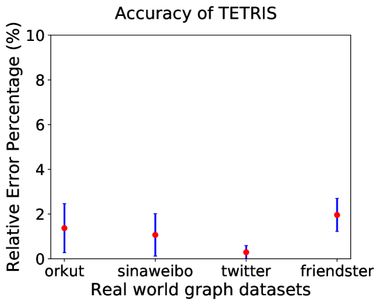
(a) We plot median relative error estimates for TETRIS on various datasets for 100 runs with fixed set of parameters. We also show the variance in the error percentage. We restrict TETRIS to visit at most 3% of the edges.

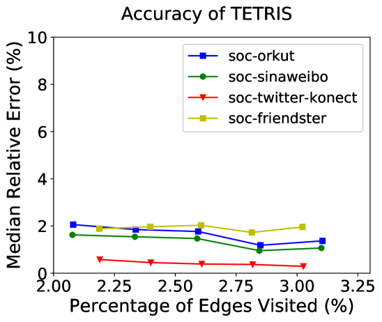
(b) we show the effect of varying the random walk length, $r$. On y-axis, we have median relative error percentage, and on x-axis we have percentage of the edges visited.

Figure 2. Accuracy of TETRIS.

Convergence.  The convergence for the orkut, weibo and twitter datasets are demonstrated in  Figure 3. We plot the final triangle estimation of TETRIS for 100 iterations for fixed choices of $s$, $r$, $\ell$, and $\operatorname{\ell_{mix}}$ (see section 5.1 for details). We increase $r$ gradually and show that the mean estimation tightly concentrates around the true triangle count. Observe that the spread of our estimator is less than 5% around the true triangle count even when we explore just 3% of the graph.

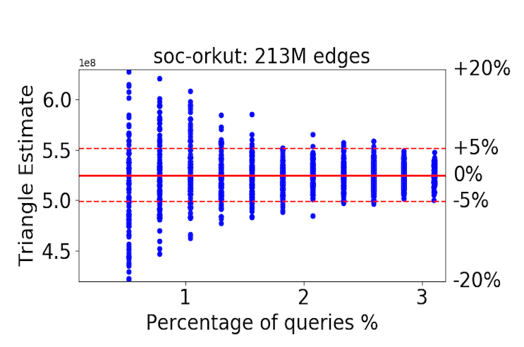
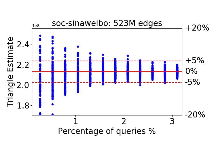
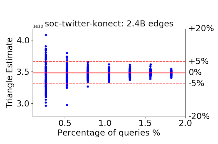
Figure 3. Convergence of TETRIS. We plot on the y-axis, the final output of TETRIS for each of the 100 runs corresponding to fixed value of $r$. On x-axis, we show the percentage of the queries made by TETRIS during its execution by increasing $r$. The maximum observed edge percentage corresponding to largest setting of $r$ is 3%.

Robustness against the choice of seed vertex.  In the previous set of experiments, we selected a fixed uniform random vertex as $s$. Surprisingly, we show that TETRIS performs almost identically regardless of the choice of seed vertex. We partition the vertices into multiple buckets according to their degree: the $i$-th group contains vertices with degree between $10^{i}$ and $10^{i+1}$. Then, from each bucket, we select $4$ vertices uniformly at random, and repeat TETRIS $100$ times for a fixed choice of $r$.

In  Figure 4, we plot the results for the orkut and the twitter datasets. On the x-axis, we consider $4$ vertices from each degree based vertex bucket for a total of $16$ vertices. On the y-axis, we plot the relative median error percentage of TETRIS for 100 independent runs starting with the corresponding vertex on the x-axis as the seed vertex $s$. The choice of $r$ leads to observing 3% of the graph. As we observe, the errors are consistently small irrespective of whether TETRIS starts its random walk from a low degree vertex or a high degree vertex. The same behavior persists across datasets for varying $r$.

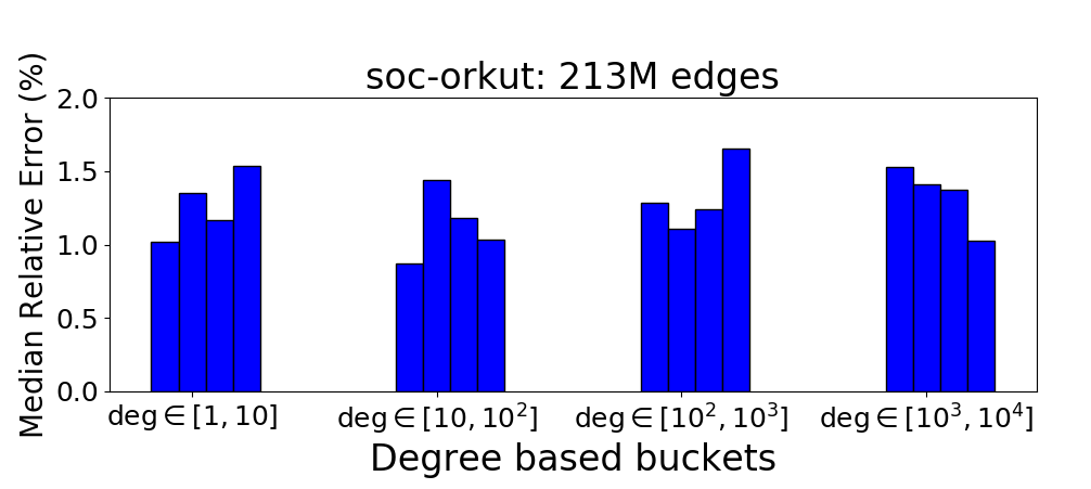
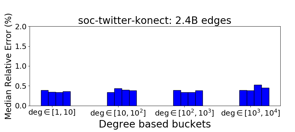
Figure 4. Robustness of TETRIS. We select 4 vertices uniformly randomly from each degree based vertex bucket. On y-axis, we show the median relative error for 100 runs of TETRIS with corresponding vertex as the seed vertex. The parameters $r$ and $\ell$ are fixed, and results in 3% of the edges being visited.

5.3. Comparison against Previous Works

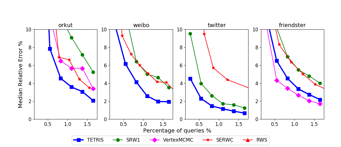
Figure 5. Comparison against baseline. For each dataset and for each parameter setting, we run all the algorithms 100 times using the same randomly chosen seed vertex. We compare the median relative error in estimation vs the percentage of queries made. The median error of RWS does not drop below 10% for any of the datasets.

We compare TETRIS against the following four benchmark algorithms. The first two algorithms are state-of-the-art in the random walk access model. The other two algorithms are simulations of widely popular uniform random edge sampling based algorithms in our model (recall that uniform random edge samples are unavailable in our model).

1. VertexMCMC ((Rahman and Hasan, 2014)): Rahman et al. in  (Rahman and Hasan, 2014) proposed multiple Metropolis-Hastings algorithms, and VertexMCMC is the best amongst them for counting triangles. In this procedure, at each step of the random walk, two neighbors of the current vertex are sampled uniformly at random and tested for the existence of a triangle. A final count is derived by scaling by the empirical success probability of finding a triangle.

2. Subgraph Random Walk (SRW (Chen et al., 2016)): Chen et al. in  (Chen et al., 2016) proposed SRW1CSS in which every three consecutive vertices on the random walk is tested for the existence of a triangle.

3. Random Walk Sparsifier (RWS): This algorithm is based on the graph sparsification strategy of  (Tsourakakis et al., 2009). It performs a random walk and counts the number of triangles in the multi-graph induced by the edges collected during the walk (with appropriate normalization).

4. Sample Edge by Random Walk and Count (SERWC): This algorithm is similar in spirit to that of (Wu et al., 2016). It counts the number of triangles incident on each edge of the random walk and outputs a scaled average as the final estimate. We note that SERWC relies on counting the number of triangles incident on an edge — a non-trivial task in our model. To make a fair comparison, we allow it to make neighbor queries: given $v\in V$ and an integer $i$, return the $i$-th neighbor of $v$, if available, else return $\emptyset$. These queries are counted towards final accounting.

We plot our comparison in Figure 5 for each of the four datasets. TETRIS is consistently accurate over all the datasets. VertexMCMC has better accuracy on the friendster dataset, however on weibo and twitter it has more than 10% error even with 1.5% queries. In contrast, TETRIS converges to an error of less than 2% with the same amount of queries. We also observe that RWS does not converge at all, and its error is more than 10%. (Essentially, the edges collected by the random walk are too correlated for standard estimators to work.) We note that SRW is also consistent across all datasets, though TETRIS significantly outperforms it on all datasets.

Normalization Factor.  Other than VertexMCMC, all the remaining algorithms require an estimate for the number of edges in the graph. VertexMCMC requires the wedge count $\sum_{v\in V}\binom{d_{v}}{2}$. While such estimates are readily available in various models, the random walk access model does not reveal this information easily. We use the EdgeCountEstimator algorithm with collected edge samples to estimate $m$ for each algorithm that requires an estimate for $m$. To estimate wedge count, we build a simple unbiased estimator (recall that the degree of each of the vertices explored by VertexMCMC is available for free).

Appendix A Proof of Theorem 4.1

The proof of the Theorem 4.1 follows directly from the Theorem 3.1 of (Ron and Tsur, 2016). For the sake of completeness, we include the proof here.

Proof of Theorem 4.1.

We begin with the estimation of $\hbox{\bf E}[c_{i}]$ and $\hbox{\bf Var}[c_{i}]$. Assume for each $1\leqslant j<k\leqslant|R_{i}|$, $c_{j,k}$ be the indicator random variable that is set to $1$ if the $j$-th and $k$-th element in $R_{i}$ are same. Then,

$$\hbox{\bf E}[c_{i}]=\sum_{(j,k):i\neq j}\hbox{\bf E}[c_{j,k}]=\frac{1}{m}\cdot\binom{|R_{i}|}{2}\,.$$

Now we turn to variance estimation. Note that each edge in the set $R_{i}$ is $\widehat{\operatorname{\ell_{mix}}}\geqslant\operatorname{\ell_{mix}}$ many steps apart in the set $R$, and hence are independent. We have, $\hbox{\bf Var}[c_{i}]=\hbox{\bf E}[c_{i}^{2}]-(\hbox{\bf E}[c_{i}])^{2}$. Now, $\hbox{\bf E}[c_{i}^{2}]=\sum_{i<j,k<l}\hbox{\bf E}[c_{ij}c_{kl}]$. Expanding the summations, we get three types of random variables: (1) $c_{ij}^{2}$ (2) $c_{ij}\cdot c_{kl}$ with exactly three distinct indices among $i,j,k,l$, and (3) $c_{ij}\cdot c_{kl}$ with all four distinct indices $i,j,k,l$. For the first type, $\hbox{\bf E}[c_{ij}^{2}]=1/m$. For the remaining two type, $\hbox{\bf E}[c_{ij}\cdot c_{kl}]=1/m^{2}$. Plugging in these terms, we get

$$\hbox{\bf Var}[c_{i}] =O\left(\frac{|R_{i}|^{2}}{m}+\frac{|R_{i}|^{3}}{m^{2}}\right)\,.$$

Then, we apply the Chebyshev Inequality in Theorem 3.2 and get

$$\Pr[c_{i}\notin(1\pm\varepsilon)\hbox{\bf E}[c_{i}]]\leqslant O\left(\frac{1}{\varepsilon^{2}}\left(\frac{m}{|R_{i}|^{2}}+\frac{1}{|R_{i}|}\right)\right)\,.$$

Plugging the the value of $|R_{i}|$, we get $Y_{i}\in(1\pm\varepsilon)m$ with constant probability. We boost the success probability with repetitions. ∎