Limit theorems for toral translations

1. Introduction

One of the surprising discoveries of dynamical systems theory is that many deterministic systems with non-zero Lyapunov exponents satisfy the same limit theorems as the sums of independent random variables. Much less is known for the zero exponent case where only a few examples have been analyzed. In this survey we consider the extreme case of toral translations where each map not only has zero exponents but is actually an isometry. These systems were studied extensively due to their relations to number theory, to the theory of integrable systems and to geometry. Surprisingly many natural questions are still open. We review known results as well as the methods to obtain them and present a list of open problems. Given a vast amount of work on this subject, it is impossible to provide a comprehensive treatment in this short survey. Therefore we treat the topics closest to our research interests in more detail while some other subjects are mentioned only briefly. Still we hope to provide the reader with the flavor of the subject and introduce some tools useful in the study of toral translations, most notably, various renormalization techniques.

Let $X={\mathbb{T}}^{d},$ $\mu$ be the Haar measure on $X$ and $T_{\alpha}(x)=x+\alpha.$

The most basic question in smooth ergodic theory is the behavior of ergodic sums. Given a map $T$ and a zero mean observable $A(\cdot)$ let

(1) $$A_{N}(x)=\sum_{n=0}^{N-1}A(T^{n}x)$$

If there is no ambiguity, we may write $A_{N}$ for $A_{N}(x)$. Conversely we may use the notation $A_{N}(\alpha,x)$ to indicate that the underlying map is the translation of vector $\alpha$. The uniform distribution of the orbit of $x$ by $T$ is characterized by the convergence to $0$ of $A_{N}(x)/N$. In the case of toral translations $T_{\alpha}$ with irrational frequency vector $\alpha$ the uniform distribution holds for all points $x.$ The study of the ergodic sums is then useful to quantify the rate of uniform distribution of the Kronecker sequence $n\alpha$ mod 1 as we will see in Section 3 where discrepancy functions are discussed. The question about the distribution of ergodic sums is analogous to the the Central Limit Theorem in probability theory. One can also consider analogues of other classical probabilistic results. In this survey we treat two such questions. In Section 4 we consider so called Poisson regime where (1) is replaced by $\sum_{n=0}^{N-1}\chi_{{\mathcal{C}}_{N}}(T_{\alpha}^{n}x)$ and the sets ${\mathcal{C}}_{N}$ are scaled in such a way that only finite number of terms are non-zero for typical $x.$ Such sums appear in several questions in mathematical physics, including quantum chaos [91] and Boltzmann-Grad limit of several mechanical systems [93]. They also describe the resonances in the study of ergodic sums for toral translations as we will see in Section 5. In Section 6 we consider Borel-Cantelli type questions where one takes a sequence of shrinking sets and studies a number of times a typical orbit hits whose sets. These questions are intimately related to some classical problems in the theory of Diophantine approximations.

The ergodic sums above toral translations also appear in natural dynamical systems such as skew products, cylindrical cascades and special flows. Discrete time systems related to ergodic sums over translations are treated in Section 7 while flows are treated in Section 8. These systems give additional motivation to study the ergodic sums (1) for smooth functions having singularities of various types: power, fractional power, logarithmic… Ergodic sums for functions with singularities are discussed in Section 2. Finally in Section 9 we present the results related to action of several translations at the same time.

Notations.

We say that a vector $\alpha=(\alpha_{1},\ldots,\alpha_{d})\in\mathbb{R}^{d}$ is irrational if $\{1,\alpha_{1},\ldots,\alpha_{d}\}$ are linearly independent over $\mathbb{Q}$.

For $x\in\mathbb{R}^{d}$, we use the notation $\{x\}:=(x_{1},\ldots,x_{d})\text{ mod }(1)$. We denote by $\|x\|$ the closest signed distance of some $x\in\mathbb{R}$ to the integers.

Assuming that $d\in\mathbb{N}$ is fixed, for $\sigma>0$ we denote by ${\mathcal{D}}(\sigma)\subset\mathbb{R}^{d}$ the set of Diophantine vectors with exponent $\sigma$, that is

(2) $${\mathcal{D}}(\sigma)=\{\alpha:\exists C\;\;\forall k\in{\mathbb{Z}}^{d}-0,m\in{\mathbb{Z}}\quad|(k,\alpha)-m|\geq C|k|^{-d-\sigma}\}$$

Let us recall that ${\mathcal{D}}(\sigma)$ has a full measure if $\sigma>0$, while ${\mathcal{D}}(0)$ is an uncountable set of zero measure and ${\mathcal{D}}(\sigma)$ is empty for $\sigma<0$. The set ${\mathcal{D}}(0)$ is called the set of constant type vector or badly approximable vectors. An irrational vector $\alpha$ that is not Diophantine for any $\sigma>0$ is called Liouville.

We denote by ${\mathfrak{C}}$ the standard Cauchy random variable with density $\frac{1}{\pi(1+x^{2})}.$ The normal random variable with zero mean and variance $D^{2}$ will be denoted by ${\mathfrak{N}}(D^{2}).$ Thus ${\mathfrak{N}}(D^{2})$ has density $\frac{1}{2\pi D}e^{-x^{2}/2D^{2}}.$ We will write simply ${\mathfrak{N}}$ for ${\mathfrak{N}}(1).$ Next, ${\mathfrak{P}}(X,\mu)$ will denote the Poisson process on $X$ with measure $\mu$ (we refer the reader to Section 5.1 for the definition and basic properties of Poisson processes).

2. Ergodic sums of smooth functions with singularities

2.1. Smooth observables

For toral translations, the ergodic sums of smooth observables are well understood. Namely if $A$ is sufficiently smooth with zero mean then for almost all $\alpha,$ $A$ is a coboundary, that is, there exists $B(\alpha,x)$ such that

(3) $$A(x)=B(x+\alpha,\alpha)-B(x,\alpha).$$

Namely if $A(x)=\sum_{k\neq 0}a_{k}e^{2\pi i(k,x)}$ then

$$B(\alpha,x)=\sum_{k\neq 0}b_{k}e^{2\pi i(k,x)}\text{ where }b_{k}=\frac{a_{k}}{e^{i2\pi(k,\alpha)}-1}.$$

The above series converges in $L^{2}$ provided $\alpha\in{\mathcal{D}}(\sigma)$ and $A\in{\mathcal{H}}^{\sigma}=\{A:\sum_{k}|a_{k}|k|^{(\sigma+d)}|^{2}<\infty\}.$ Note that (3) implies that

$$A_{N}(x,\alpha)=B(x+N\alpha,\alpha)-B(x,\alpha)$$

giving a complete description of the behavior of ergodic sums for almost all $\alpha.$ In particular we have

Corollary 1.

If $\alpha$ is uniformly distributed on ${\mathbb{T}}^{d}$ then $A_{N}(x)$ has a limiting distribution as $N\to\infty,$ namely

$$A_{N}\Rightarrow B(y,\alpha)-B(x,\alpha)$$

where $(y,\alpha)$ is uniformly distributed on ${\mathbb{T}}^{d}\times{\mathbb{T}}^{d}.$

Proof.

We need to show that as $N\to\infty$ the random vector $(\alpha,N\alpha)$ converge to a vector with coordinates independent random variables uniformly distributed on ${\mathbb{T}}^{d}\times{\mathbb{T}}^{d}.$ To this end it suffices to check that if $\phi(x,y)$ is a smooth function on ${\mathbb{T}}^{d}\times{\mathbb{T}}^{d}$ then

$$\lim_{N\to\infty}\int_{{\mathbb{T}}^{d}}\phi(\alpha,N\alpha)d\alpha=\int_{{\mathbb{T}}^{d}\times{\mathbb{T}}^{d}}\phi(\alpha,\beta)d\alpha d\beta$$

but this is easily established by considering the Fourier series of $\phi.$ ∎

We will see in Section 8 how our understanding of ergodic sums for smooth functions can be used to derive ergodic properties of area preserving flows on $\mathbb{T}^{2}$ without fixed points.

On the other hand there are many open questions related to the case when the observable $A$ is not smooth enough for (3) to hold. Below we mention several classes of interesting observables.

2.2. Observables with singularities

Special flows above circle rotations and under ceiling functions that are smooth except for some singularities naturally appear in the study of conservative flows on surfaces with fixed points.

Another motivation for studying ergodic sums for functions with singularities is the case of meromorphic functions, whose sums appear in questions related to both number theory [48] and ergodic theory [106].

2.2.1. Observables with logarithmic singularities.

In the study of conservative flows on surfaces, non degenerate saddle singularities are responsible for logarithmic singularities of the ceiling function.

Ceiling functions with logarithmic singularities also appear in the study of multi-valued Hamiltonians on the two torus. In [3], Arnold investigated such flows and showed that the torus decomposes into cells that are filled up by periodic orbits and one open ergodic component. On this component, the flow can be represented as a special flow over an interval exchange map of the circle and under a ceiling function that is smooth except for some logarithmic singularities. The singularities can be asymmetric since the coefficient in front of the logarithm is twice as big on one side of the singularity as the one on the other side, due to the existence of homoclinic loops (see Figure 1).

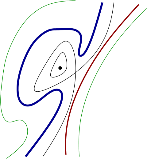
Figure 1. Multivalued Hamiltonian flow. Note that the orbits passing to the left of the saddle spend approximately twice longer time comparing to the orbits passing to the right of the saddle and starting at the same distance from the separatrix since they pass near the saddle twice.

More motivations for studying function with logarithmic singularities as well as some numerical results for rotation numbers of bounded type are presented in [69].

A natural question is to understand the fluctuations of the ergodic sums for these functions as the frequency $\alpha$ of the underlying rotation is random as well as the base point $x$. Since Fourier coefficients of the symmetric logarithm function have the asymptotics similar to that of the indicator function of an interval one may expect that the results about the latter that we will discuss in Section 3 can be extended to the former.

Question 1.

Suppose that $A$ is smooth away from a finite set of points $x_{1},x_{2}\dots x_{k}$ and near $x_{j},$ $A(x)=a_{j}^{\pm}\ln|x-x_{j}|+r_{j}(x)$ where $-$ sign is taken if $x<x_{j},$ $+$ sign is taken if $x>x_{j}$ and $r_{j}$ are smooth functions. What can be said about the distribution of $A_{N}(\alpha,x)/\ln N$ as $x$ and $\alpha$ are random?

2.2.2. Observables with power like singularities.

When considering conservative flows on surfaces with degenerate saddles one is led to study the ergodic sums of observables with integrable power like singularities (more discussion of these flows will be given in Section 8). Special flows above irrational rotations of the circle under such ceiling functions are called Kocergin flows.

The study of ergodic sums for smooth ergodic flows with nondegenerate hyperbolic singular points on surfaces of genus $p\geq 2$ shows that these flows are in general not mixing (see Section 8). A contrario Kocergin showed that special flows above irrational rotations and under ceiling functions with integrable power like singularities are always mixing. This is due to the important deceleration next to the singularity that is responsible for a shear along orbits that separates the points sufficiently to produce mixing. In other words, the mixing is due to large oscillations of the ergodic sums. In this note we will be frequently interested in the distribution properties of these sums.

One may also consider the case of non-integrable power singularities since they naturally appear in problems of ergodic theory and number theory. The following result answers a question of [48].

Theorem 2.

([120]) If $A$ has one simple pole on ${\mathbb{T}}^{1}$ and $(\alpha,x)$ is uniformly distributed on ${\mathbb{T}}^{2}$ then $\frac{A_{N}}{N}$ has a limiting distribution as $N\to\infty.$

The function $A$ in Theorem 2 has a symmetric singularity of the form $1/x$ that is the source of cancellations in the ergodic sums.

Question 2.

What happens for an asymmetric singularity of the type $1/|x|$?

Question 3.

What happens in the quenched setting where $\alpha$ is fixed?

We now present several generalizations of Theorem 2.

Theorem 3.

Let $A=\tilde{A}(x)+\frac{c_{-}\chi_{x<x_{0}}+c^{+}\chi_{x>x_{0}}}{|x-x_{0}|^{a}}$ where $\tilde{A}$ is smooth and $a>1.$

(a) If $(\alpha,x)$ is uniformly distributed on ${\mathbb{T}}^{2}$ then $\dfrac{A_{N}}{N^{a}}$ converges in distribution.

(b) For almost every $x$ fixed, if $\alpha$ is uniformly distributed on ${\mathbb{T}}$ then $\dfrac{A_{N}(\alpha,x)}{N^{a}}$ converge to the same limit as in part (a).

Theorem 4.

[87] If $A$ has zero mean and is smooth except for a singularity at $0$ of type $|x|^{-a}$, $a\in(0,1)$ then $A_{N}/N^{a}$ converges in distribution.

The proof of Theorem 4 is inspired by the proof of Theorem 10 of Section 3 which will be presented in Section 5.5.

Marklof proved in [92] that if $\alpha\in{\mathcal{D}}(\sigma)$ with $\sigma<(1-a)/a$, then for $A$ as in Theorem 4 $A_{N}(\alpha,\alpha)/N\to 0$.

Question 4.

What happens for other angles $\alpha$ and other type of singularities, including the non integrable ones for which the ergodic theorem does not necessarily hold?

Another natural generalization of Theorem 2 is to consider meromorphic functions. Let $A$ be such a function with highest pole of order $m.$ Thus $A$ can be written as

$$A(x)=\sum_{j=1}^{r}\frac{c_{j}}{(x-x_{j})^{m}}+{\tilde{A}}(x)$$

where the highest pole of ${\tilde{A}}$ has order at most $m-1.$

Theorem 5.

(a) Let $A$ be fixed and let $\alpha$ be distributed according to a smooth density on $\mathbb{T}.$ Then for any $x\in\mathbb{T}$, $\dfrac{A_{N}(\alpha,x)}{N^{m}}$ has a limiting distribution as $N\to\infty.$

(b) Let ${\tilde{A}},c_{1},\dots c_{r}$ be fixed while $(\alpha,x,x_{1}\dots x_{r})$ are distributed according to a smooth density on on ${\mathbb{T}}^{r+2}$ then $\dfrac{A_{N}(\alpha,x)}{N^{m}}$ has a limiting distribution as $N\to\infty.$

(c) If $(x_{1},x_{2}\dots x_{r})$ is a fixed irrational vector then for almost every $x\in\mathbb{T}$ the limit distribution in part (a) is the same as the limit distribution in part (b).

Proofs of Theorems 3 and 5 are sketched in Section 5.

It will be apparent from the proof of Theorem 5 that the limit distribution in part (a) is not the same for all $x_{1},x_{2}\dots x_{j}.$ For example if $x_{j}=jx_{1}$ we get an exceptional distribution since a close approach to $x_{1}$ and $x_{2}$ by the orbit of $x$ should be followed by a close approach to $x_{j}$ for $j\geq 3.$ We will see that this phenomenon appears in many limit theorems (see e.g Theorem 9, Theorem 25 and Question 52, Theorem 38 and Question 38, as well as [93]).

Question 5.

What can be said about more general meromorphic functions such as $\sin 2\pi x/(\sin 2\pi x+3\cos 2\pi y)$ on $\mathbb{T}^{d}$ with $d>1?$

3. Ergodic sums of characteristic functions. Discrepancies

The case where $A=\chi_{\Omega}$ is a classical subject in number theory. Define the discrepancy function

$$D_{N}(\Omega,\alpha,x)=\sum_{n=0}^{N-1}\chi_{\Omega}(x+n\alpha)-N\frac{\text{Vol}(\Omega)}{\text{Vol}({\mathbb{T}}^{d})}.$$

Uniform distribution of the sequence $x+k\alpha$ on $\mathbb{T}^{d}$ is equivalent to the fact that, for regular sets $\Omega,$ $D_{N}(\Omega,\alpha,x)/N\to 0$ as $N\to\infty$. A step further in the description of the uniform distribution is the study of the rate of convergence to $0$ of $D_{N}(\Omega,\alpha,x)/N$.

In $d=1$ it is known that if $\alpha\in\mathbb{T}-\mathbb{Q}$ is fixed, the discrepancy $D_{N}(\Omega,\alpha,x)/N$ displays an oscillatory behavior according to the position of $N$ with respect to the denominators of the best rational approximations of $\alpha$. A great deal of work in Diophantine approximation has been done on estimating the discrepancy function in relation with the arithmetic properties of $\alpha\in\mathbb{T}$, and more generally for $\alpha\in\mathbb{T}^{d}$.

3.1. The maximal discrepancy

Let

(4) $$\overline{D}_{N}(\alpha)=\sup_{\Omega\in\mathbb{B}}D_{N}(\Omega,\alpha,0)$$

where the supremum is taken over all sets $\Omega$ in some natural class of sets $\mathbb{B}$, for example balls or boxes (product of intervals).

The case of (straight) boxes was extensively studied, and growth properties of the sequence $\overline{D}_{N}(\alpha)$ were obtained with a special emphasis on their relations with the Diophantine approximation properties of $\alpha.$ In particular, following earlier advances of [75, 48, 99, 64, 117] and others, [8] proves

Theorem 6.

Let

$$\overline{D}_{N}(\alpha)=\sup_{\Omega-\text{box}}D_{N}(\Omega,\alpha,0)$$

Then for any positive increasing function $\phi$ we have

(5) $$\hskip 11.38092pt\sum_{n}\phi(n)^{-1}<\infty\iff\frac{\overline{D}_{N}(\alpha)}{(\ln N)^{d}\phi(\ln\ln N)}\begin{array}[]{l}\text{ is bounded for}\\ \text{ almost every }\alpha\in\mathbb{T}^{d}.\end{array}$$

In dimension $d=1$, this result is the content of Khinchine theorems obtained in the early 1920’s [64], and it follows easily from well-known results from the metrical theory of continued fractions (see for example the introduction of [8]). The higher dimensional case is significantly more difficult and the cited bound was only obtained in the 1990s.

The bound in (5) focuses on how bad can the discrepancy become along a subsequence of $N$, for a fixed $\alpha$ in a full measure set. In a sense, it deals with the worst case scenario and does not capture the oscillations of the discrepancy. On the other hand, the restriction on $\alpha$ is necessary, since given any ${\varepsilon}_{n}\to 0$ it is easy to see that for $\alpha\in\mathbb{T}$ sufficiently Liouville, the discrepancy (relative to intervals) can be as bad as $N_{n}{\varepsilon}_{n}$ along a suitable sequence $N_{n}$ (large multiples of Liouville denominators).

For $d=1$, it is not hard to see, using continued fractions, that for any $\alpha$ : $\limsup\frac{\overline{D}_{N}(\alpha)}{\ln N}>0$, $\liminf\overline{D}_{N}(\alpha)\leq C$; and for $\alpha\in\mathcal{D}(0)$ $\limsup\frac{\overline{D}_{N}(\alpha)}{\ln N}<+\infty$. The study of higher dimensional counterparts to these results raises several interesting questions.

Question 6.

Is it true that $\limsup\frac{\overline{D}_{N}(\alpha)}{\ln^{d}N}>0$ for all $\alpha\in{\mathbb{T}}^{d}$?

Question 7.

Is it true that there exists $\alpha$ such that $\limsup\frac{\overline{D}_{N}(\alpha)}{\ln^{d}N}<+\infty$?

Question 8.

What can one say about $\liminf\frac{\overline{D}_{N}(\alpha)}{a_{N}}$ for a.e. $\alpha$, where $a_{N}$ is an adequately chosen normalization? for every $\alpha$?

Question 9.

Same questions as Questions 6–8 when boxes are replaced by balls.

Question 10.

Same questions as Questions 6–8 for the isotropic discrepancy, when boxes are replaced by the class of all convex sets [79].

3.2. Limit laws for the discrepancy as $\alpha$ is random

In this survey, we will mostly concentrate on the distribution of the discrepancy function as $\alpha$ is random. The above discussion naturally raises the following question.

Question 11.

Let $\alpha$ be uniformly distributed on $\mathbb{T}^{d}.$ Is it true that $\frac{\overline{D}_{N}(\alpha)}{\ln^{d}N}$ converges in distribution as $N\to\infty$?

Why do we need to take $\alpha$ random? The answer is that for fixed $\alpha$ the discrepancy does not have a limit distribution, no water which normalization is chosen.

For example for $d=1$ the Denjoy-Koksma inequality says that

$$|A_{q_{n}}-q_{n}\int A(x)dx|\leq 2V$$

where $q_{n}$ is the $n$-th partial convergent to $\alpha$ and $V$ denotes the total variation of $A.$ In particular $D_{q_{n}}(I,\alpha,x)$ can take at most 3 values.

In higher dimensions one can show that if $\Omega$ is either a box or any other strictly convex set then for almost all $\alpha$ and almost all tori, when $x$ is random the variable

$$\frac{D_{N}(\Omega,{\mathbb{R}}^{d}/L,\alpha,\cdot)}{a_{N}}$$

does not converge to a non-trivial limiting distribution for any choice of $a_{N}=a_{N}(\alpha,L)$ (see discussion in the introduction of [29]).

Question 12.

Is this true for all $\alpha,L$?

Question 13.

Study the distributions which can appear as weak limits of $\dfrac{D_{N}(\Omega,\alpha,\cdot)}{a_{N}}$, in particular their relation with number theoretic properties of $\alpha.$

Let us consider the case $d=1$ (so the sets of interest are intervals and we will write $I$ instead of $\Omega$.) It is easy to see that all limit distributions are atomic for all $I$ iff $\alpha\in{\mathbb{Q}}.$

Question 14.

Is it true that all limit distributions are either atomic or Gaussian for almost all $I$ iff $\alpha$ is of bounded type?

Evidence for the affirmative answer is contained in the following results.

Theorem 7.

([55]) If $\alpha\not\in{\mathbb{Q}}$ and $I=[0,1/2]$ then there is a sequence $N_{j}$ such that $\dfrac{D_{N_{j}}(I,\alpha,\cdot)}{j}$ converges to ${\mathfrak{N}}.$

Instead of considering subsequences, it is possible to randomize $N.$

Theorem 8.

Let $\alpha$ be a quadratic surd.

(a) ([10]) If $(x,a,l)$ is uniformly distributed on ${\mathbb{T}}^{3}$ then $\dfrac{D_{[aN]}([0,l],\alpha,x)}{\sqrt{\ln N}}$ converges to ${\mathfrak{N}}(\sigma^{2})$ for some $\sigma^{2}\neq 0.$

(b) ([11]) If $M$ is uniformly distributed on $[1,N]$ and $l$ is rational then there are constants $C(\alpha,l),\sigma(\alpha,l)$ such that $\dfrac{D_{M}([0,l],\alpha,0)-C(\alpha,l)\ln N}{\sqrt{\ln N}}$ converges to ${\mathfrak{N}}(\sigma^{2}(\alpha,l)).$

Note that even though we have normalized the discrepancy by subtracting the expected value an additional normalization is required in Theorem 8(b). The reason for this is explained at the end of Section 8.5.

So if one wants to have a unique limit distribution for all $N$ one needs to allow random $\alpha.$

The case when $d=1$ was studied by Kesten. Define

$$V(u,v,w)=\sum_{k=1}^{\infty}\frac{\sin(2\pi u)\sin(2\pi v)\sin(2\pi w)}{k^{2}}.$$

If $(r,q)$ are positive integers let

$$\theta(r,q)=\frac{{\mathrm{Card}}(j:0\leq j\leq q-1:gcd(j,r,q)=1)}{{\mathrm{Card}}(j,k:0\leq j,k\leq q-1:gcd(j,k,q)=1)}.$$

Finally let

$$c(r)=\begin{cases}\frac{\pi^{3}}{12}\left[\sum_{r=0}^{q-1}\theta(p,q)\int_{0}^{1}\int_{0}^{1}V(u,\frac{rp}{q},v)dudv\right]^{-1}&\text{if }r=\frac{p}{q}\text{ and }gcd(p,q)=1\\ \frac{\pi^{3}}{12}\left[\int_{0}^{1}\int_{0}^{1}\int_{0}^{1}V(u,r,v)dudrdv\right]^{-1}&\text{if }r\text{ is irrational.}\end{cases}$$

Theorem 9.

([61, 62]) If $(\alpha,x)$ is uniformly distributed on ${\mathbb{T}}^{2}$ then $\frac{D_{N}([0,l],\alpha,x)}{c(l)\ln N}$ converges to the Cauchy distribution ${\mathfrak{C}}.$

Note that the normalizing factor is discontinuous as a function of the length of the interval at rational values.

A natural question is to extend Theorem 9 to higher dimensions. The first issue is to decide which sets $\Omega$ to consider instead of intervals. It appears that a quite flexible assumption is that $\Omega$ is semialgebraic, that is, it is defined by a finite number of algebraic inequalities.

Question 15.

Suppose that $\Omega$ is semialgebraic then there is a sequence $a_{N}=a_{N}(\Omega)$ such that for a random translation of a random torus $\dfrac{D_{N}(\Omega,{\mathbb{R}}^{d}/L,\alpha,x)}{a_{N}}$ converges in distribution as $N\to\infty.$

By random translation of a random torus, we mean a translation of random angle $\alpha$ on a torus ${\mathbb{R}}^{d}/L$ where $L=A{\mathbb{Z}}^{d}$ and the triple $(\alpha,x,A)$ has a smooth density on ${\mathbb{T}}^{d}\times{\mathbb{T}}^{d}\times\text{GL}(\mathbb{R},d)$. Notice that comparing to Kesten’s result of Theorem 9, Question 15 allows for additional randomness, namely, the torus is random. In particular, for $d=1$, the study of the discrepancy of visits to $[0,l]$ on the torus ${\mathbb{R}}/{\mathbb{Z}}$ is equivalent to the study of the discrepancy of visits to $[0,1]$ on the torus ${\mathbb{R}}/(l^{-1}{\mathbb{Z}}).$ Thus the purpose of the extra randomness is to avoid the irregular dependence on parameters observed in Theorem 9 (cf. also [109, 110]).

So far Question 15 has been answered for two classes of sets which are natural counterparts to intervals in higher dimensions : strictly convex sets and (tilted) boxes.

Given a convex body $\Omega$, we consider the family $\Omega_{r}$ of bodies obtained from $\Omega$ by rescaling it with a ratio $r>0$ (we apply to $\Omega$ the homothety centered at the origin with scale $r$). We suppose $r<r_{0}$ so that the rescaled bodies can fit inside the unit cube of $\mathbb{R}^{d}$. We define

(6) $$D_{N}(\Omega,r,\alpha,x)=\sum_{n=0}^{N-1}\chi_{\Omega_{r}}(x+n\alpha)-N{\rm Vol}({\Omega_{r}})$$

Theorem 10.

([28]) If $(r,\alpha,x)$ is uniformly distributed on $X=[a,b]\times\mathbb{T}^{d}\times\mathbb{T}^{d}$ then $\frac{D_{N}(\Omega,r,\alpha,x)}{r^{(d-1)/2}N^{(d-1)/2d}}$ has a limit distribution as $N\to\infty.$

The form of the limiting distribution is given in Theorem 18 in Section 5.

In the case of boxes we recover the same limit distribution as in Kesten but with a higher power of the logarithm in the normalization.

Theorem 11.

([29]) In the context of Question 15, if $\Omega$ is a box, then $\dfrac{D_{N}}{c\ln^{d}N}$ converges to ${\mathfrak{C}}$ as $N\to\infty.$

Alternatively, one can consider gilded boxes, namely: for $u=(u_{1},\ldots,u_{d})$ with $0<u_{i}<1/2$ for every $i$, we define a cube on the $d$-torus by $C_{u}=[-u_{1},u_{1}]\times\ldots[-u_{d},u_{d}]$. Let $\eta>0$ and $MC_{u}$ be the image of $C_{u}$ by a matrix $M\in{\rm SL}(d,\mathbb{R})$ such that

$$M=(a_{ij})\in G_{\eta}=\{|a_{i,i}-1|<\eta,\text{ for every }i\text{ and }|a_{i,j}|<\eta\text{ for every }j\neq i\}.$$

For a point $x\in\mathbb{T}^{d}$ and a translation frequency vector $\alpha\in\mathbb{T}^{d}$ we denote $\xi=(u,M,\alpha,x)$ and define the following discrepancy function

$$D_{N}(\xi)=\#\{1\leq m\leq N:(x+m\alpha){\rm\ mod\ }1\in MC_{u}\}-2^{d}\left(\Pi_{i}u_{i}\right)N.$$

Fix $d$ segments $[v_{i},w_{i}]$ such that $0<v_{i}<w_{i}<1/2\forall i=1,\ldots,d$. Let

(7) $$X=(u,\alpha,x,(a_{i,j}))\in[v_{1},w_{1}]\times\dots[v_{d},w_{d}]\times\mathbb{T}^{2d}\times G_{\eta}$$

We denote by ${\mathbb{P}}$ the normalized restriction of the Lebesgue $\times$ Haar measure on $X$. Then, the precise statement of Theorem 11 is

Theorem 12.

([29]) Let $\rho=\frac{1}{d!}\left(\frac{2}{\pi}\right)^{2d+2}.$ If $\xi$ is distributed according to $\lambda$ then $\frac{D_{N}(\xi)}{\rho(\ln N)^{d}}$ converges to ${\mathfrak{C}}$ as $N\to\infty.$

Question 16.

Are Theorems 10–12 valid if

(a) The lattice $L$ is fixed; (b) $x$ is fixed?

Question 17.

Describe large deviations for $D_{N}.$ That is, given $b_{N}\gg a_{N}$ where $a_{N}$ is the same as in Question 15, study the asymptotics of ${\mathbb{P}}(D_{N}\geq b_{N}).$ One can study this question in the annealed setting when all variables are random or in the quenched setting where some of them are fixed.

Question 18.

Does a local limit theorem hold? That is, is it true that given a finite interval $J$ we have

$$\lim_{N\to\infty}a_{N}{\mathbb{P}}(D_{N}\in J)=c|J|?$$

4. Poisson regime

The results presented in the last section deal with the so called CLT regime. This is the regime when, since the target set $\Omega$ is macroscopic (having volume of order $1$), if $T$ was sufficiently mixing, one would get the Central Limit Theorem for the ergodic sums of $\chi_{\Omega}$. In this section we discuss Poisson (microscopic) regime, that is, we let $\Omega=\Omega_{N}$ shrink so that ${\mathbb{E}}(D_{N}(\Omega_{N},\alpha,x))$ is constant. In this case, the sum in the discrepancy consists of a large number of terms each one of which vanishes with probability close to 1 so that typically only finitely many terms are non-zero.

Theorem 13.

([88]) Suppose that $\Omega$ is a bounded set whose boundary has zero measure.

If $(\alpha,x)$ is uniformly distributed on ${\mathbb{T}}^{d}\times{\mathbb{T}}^{d}$ then both $D_{N}(N^{-1/d}\Omega,\alpha,x)$ and $D_{N}(N^{-1/d}\Omega,\alpha,0)$ converge in distribution.

Note that in this case the result is less sensitive to the shape of $\Omega$ than in the case of sets of unit size.

We will see later (Theorem 16 in Section 5) that one can also handle several sets at the same time.

Corollary 14.

If $(\alpha,x)$ is uniformly distributed on ${\mathbb{T}}^{d}\times{\mathbb{T}}^{d}$ then the following random variables have limit distributions

(a) $\displaystyle N^{1/d}\min_{0\leq n<N}d(x+n\alpha,\bar{x})$ where $\bar{x}$ is a given point in $\mathbb{T}^{d};$

(b) $\displaystyle N^{2/d}\min_{0\leq n<N}[A(x+n\alpha)-A(\bar{x})]$ where $A$ is a Morse function with minimum at $\bar{x}.$

Proof.

To prove (a) note that $\displaystyle N^{1/d}\min_{0\leq n<N}d(x+n\alpha,\bar{x})\leq s$ iff the number of points of the orbit of $x$ of length $N$ inside $B(\bar{x},sN^{-1/d})$ is zero.

To prove (b) note that if $A$ is a Morse function and x is close to $\bar{x}$ then $A(x)\approx A(\bar{x})+(D^{2}A)(\bar{x})(x-\bar{x},x-\bar{x}).$ ∎

There are two natural ways to extend this result.

Question 19.

If $S\subset\mathbb{T}^{d}$ is an analytic submanifold of codimension $q$ find the limit distribution of $\displaystyle N^{1/q}\min_{0\leq n<N}d(x+n\alpha,S).$

Question 20.

Given a typical analytic function $A$ find a limit distribution of $\displaystyle N^{\frac{1}{d}}\min_{0\leq n<N}|A(x+n\alpha)|.$

As we shall see in Section 5.4 this question is closely related to Question 5.

5. Outlines of proofs

5.1. Poisson processes

In this section we recall some facts about the Poisson processes referring the reader to [93, Section 11] or [65] for more details. The next section contains preliminaries from homogenous dynamics.

Recall that a random variable $N$ has Poisson distribution with parameter $\lambda$ if ${\mathbb{P}}(N=k)=e^{-\lambda}\frac{\lambda_{k}}{k!}.$ Now an easy combinatorics shows the following facts

(I) If $N_{1},N_{2}\dots N_{m}$ are independent random variables and $N_{j}$ have Poisson distribution with parameters $\lambda_{j}$, then $N=\sum_{j=1}^{m}N_{j}$ has Poisson distribution with parameter $\sum_{j=1}^{m}\lambda_{j}.$

(II) Conversely, take $N$ points distributed according to a Poisson distribution with parameter $\lambda$ and color each point independently with one of $m$ colors where color $j$ is chosen with probability $p_{j}.$ Let $N_{j}$ be the number of points of color $j.$ Then $N_{j}$ are independent and $N_{j}$ has Poisson distribution with parameter $\lambda_{j}=p_{j}\lambda.$

Now let $(\Omega,\mu)$ be a measure space. By a Poisson process on this space we mean a random point process on $X$ such that if $\Omega_{1},\Omega_{2}\dots\Omega_{m}$ are disjoint sets and $N_{j}$ is the number of points in $\Omega_{j}$ then $N_{j}$ are independent Poisson random variables with parameters $\mu(\Omega_{j})$ (note that this definition is consistent due to (I)). We will write $\{x_{j}\}\sim{\mathfrak{P}}((X,\mu))$ to indicate that $\{x_{j}\}$ is a Poisson process with parameters $(X,\mu).$ If $(X,\mu)=(\mathbb{R},c{\mathrm{Leb}})$ we shall say that $X$ is a Poisson process with intensity $c.$ The following properties of the Poisson process are straightforward consequences of (I) and (II) above.

Proposition 1.

(a) If $\{x_{j}^{\prime}\}\sim{\mathfrak{P}}(X,\mu^{\prime})$ and $\{x_{j}^{\prime\prime}\}\sim{\mathfrak{P}}(X,\mu^{\prime\prime})$ are independent then $\{x_{j}^{\prime}\}\cup\{x_{j}^{\prime\prime}\}\sim{\mathfrak{P}}(X,\mu^{\prime}+\mu^{\prime\prime}).$

(b) If $\{x_{j}\}\sim{\mathfrak{P}}(X,\mu)$ and $f:X\to Y$ is a measurable map then $\{f(x_{j})\}\sim{\mathfrak{P}}(Y,f^{-1}\mu).$

(c) Let $X=Y\times Z,$ $\mu=\nu\times\lambda$ where $\lambda$ is a probability measure on $Z.$ Then $\{(y_{j},z_{j})\}\sim{\mathfrak{P}}(X,\mu)$ iff $\{y_{j}\}\sim{\mathfrak{P}}(Y,\nu)$ and $z_{j}$ are random variables independent from $\{y_{j}\}$ and each other and distributed according to $\lambda.$

Next recall [40, Chapter XVII] that the Cauchy distribution is unique (up to scaling) symmetric distribution such that if $Z,Z^{\prime}$ and $Z^{\prime\prime}$ are independent random variables with that distribution then $Z^{\prime}+Z^{\prime\prime}$ has the same distribution as $2Z.$ We have the following representation of the Cauchy distribution.

Proposition 2.

(a) If $\{x_{j}\}$ is a Poisson process with constant intensity then $\sum_{j}\frac{1}{x_{j}}$ has Cauchy distribution. (the sum is understood in the sense of principle value).

(b) If $\{x_{j}\}$ is a Poisson distribution with constant intensity and $\xi_{j}$ are random variables with finite expectation independent from $\{x_{j}\}$ and from each other then

(8) $$\sum_{j}\frac{\xi_{j}}{x_{j}}$$

has Cauchy distribution.

To see part (a) let $\{x_{j}^{\prime}\},\{x_{j}^{\prime\prime}\}$ and $\{x_{j}\}$ are independent Poisson processes with intensity $c.$ Then

$$\sum\frac{1}{x_{j}^{\prime}}+\sum\frac{1}{x_{j}^{\prime\prime}}=\sum_{y\in\{x_{j}^{\prime}\}\cup\{x_{j}^{\prime\prime}\}}\frac{1}{y}$$

and by Proposition 1 (a) and (b) both $\{x_{j}^{\prime}\}\cup\{x_{j}^{\prime\prime}\}$ and $\{\frac{x_{j}}{2}\}$ are Poisson processes with intensity $2c.$

To see part (b) note that by Proposition 1(b) and (c), $\{\frac{x_{j}}{\xi_{j}}\}$ is a Poisson process with constant intensity.

5.2. Uniform distribution on the space of lattices

In order to describe ideas of the proofs from Sections 2, 3, and 4 we will first go over some preliminaries. By a random $d$-dimensional lattice (centered at 0) we mean a lattice $L=Q\mathbb{Z}^{d}$ where $Q$ is distributed according to Haar measure on $G=SL_{d}(\mathbb{R})/SL_{d}(\mathbb{Z}).$

By a random $d$-dimensional affine lattice we mean an affine lattice $L=Q\mathbb{Z}^{d}+b$ where $(Q,b)$ is distributed according to a Haar measure on $\bar{G}=(SL_{d}(\mathbb{R})\ltimes\mathbb{R}^{d})/(SL_{d}(\mathbb{Z})\ltimes\mathbb{Z}^{d}).$ Here $\bar{G}$ is equipped with the multiplication rule $(A,a)(B,b)=(AB,a+Ab)$.

We denote by $g_{t}$ the diagonal action on $G$ given by

$$g^{t}=\left(\begin{array}[]{llll}e^{t/d}&\dots&0&0\\ &&&\\ 0&\dots&e^{t/d}&0\\ 0&\dots&0&e^{-t}\end{array}\right)$$

and for $\alpha\in\mathbb{R}^{d-1}$ we denote by $\Lambda_{\alpha}$ the horocyclic action

(9) $$\Lambda_{\alpha}=\left(\begin{array}[]{llll}1&\dots&0&\alpha_{1}\\ &&&\\ 0&\dots&1&\alpha_{d-1}\\ 0&\dots&0&1\end{array}\right).$$

The action of $g^{t}$ on the space of affine lattices $G$ is partially hyperbolic and unstable manifolds are orbits of $\Lambda_{\alpha}$ where $\alpha\in\mathbb{R}^{d-1}$.

Similarly the action by ${g}_{t}:=(g_{t},0)$, defined on the space of affine lattices is partially hyperbolic and unstable manifolds are orbits of $(\Lambda_{\alpha},\bar{x})$ where $(\alpha,x)\in(\mathbb{R}^{d-1})^{2}$ and

$$\bar{x}=\left(\begin{array}[]{l}x_{1}\\ {}\\ x_{d-1}\\ 0\end{array}\right).$$

For convenience, here and below we will use the notation $\bar{x}=(x_{1},\ldots,x_{d-1},0)$ for the column vector $x\in{\mathbb{R}}^{d-1}$.

We can also equip $SL_{d}(\mathbb{R})\ltimes(\mathbb{R}^{d})^{r}$ with the multiplication rule

(10) $$(A,a_{1},\dots,a_{r})(B,b_{1},\dots,b_{r})=(AB,a_{1}+Ab_{1},\dots,a_{r}+Ab_{r}),$$

and consider the space of periodic configurations in $d$-dimensional space $\hat{G}=SL_{d}(\mathbb{R})\ltimes(\mathbb{R}^{d})^{r}/SL_{d}(\mathbb{Z})\ltimes(\mathbb{Z}^{d})^{r}$.

The action of $g_{t}:=(g^{t},0,\ldots,0)$ on $\hat{G}$ is partially hyperbolic and unstable manifolds are orbits of $(\Lambda_{\alpha},\bar{x}_{1},\ldots,\bar{x}_{r})$ where $\alpha,\bar{x}_{j}\in\mathbb{R}^{d-1}$.

We will denote these unstable manifolds by $n_{+}(\alpha)$ or $n_{+}(\alpha,\bar{x})$ or $n_{+}(\alpha,\bar{x}_{1},\ldots,\bar{x}_{r})$. Note also that $n_{+}(\alpha,\bar{x})$ or $n_{+}(\alpha,\bar{x}_{1},\ldots,\bar{x}_{r})$ for fixed $\bar{x},\bar{x}_{1},\ldots,\bar{x}_{r}$ form positive codimension manifolds inside the full unstable leaves of the action of $g_{t}$.

We will often use the uniform distribution of the images of unstable manifolds for partially hyperbolic flows (see e.g. [33]) to assert that $g_{t}(\Lambda_{\alpha})$ or $g_{t}(\Lambda_{\alpha},\bar{x})$ or $g_{t}(\Lambda_{\alpha},\bar{x}_{1},\ldots,\bar{x}_{r})$ becomes uniformly distributed in the corresponding lattice spaces according to their Haar measures as $\alpha,\bar{x},\bar{x}_{1},\ldots,\bar{x}_{r}$ are independent and distributed according to any absolutely continuous measure on $\mathbb{R}^{d-1}$. In fact, if the original measure has smooth density, then one has exponential estimate for the rate of equidistribution (cf. [66]). The explicit decay estimates play an important role in proving limit theorems by martingale methods. For example, such estimates are helpful in proving Theorem 9 in Section 3 and Theorems 26, 27 in Section 6.

Below we shall also encounter a more delicate situation when all or some of $\bar{x},\bar{x}_{j}$ are fixed so we have to deal with positive codimension manifolds inside the full unstable horocycles. In this case one has to use Ratner classification theory for unipotent actions. Examples of unipotent actions are $n_{+}(\cdot)$ or $n_{+}(\cdot,\bar{x})$ or $n_{+}(\alpha,\cdot)$. The computations of the limiting distribution of the translates of unipotent orbits proceeds in two steps (cf. [93]). For several results described in the previous sections we need the limit distribution of $g_{t}\Lambda_{\alpha}w$ inside $X={\mathbf{G}}/{\boldsymbol{\Gamma}}$ where $X$ can be any of the sets $G,\bar{G},\hat{G}$ described above and $w\in{\mathbf{G}}.$ In fact, the identity $g_{t}\Lambda_{\alpha}w=w(w^{-1}g_{t}\Lambda_{\alpha}w)$ allows us to assume that $w=id$ at the cost of replacing the action of $SL_{d}(\mathbb{R})$ by right multiplication by a twisted action $\phi_{w}(M)u=w^{-1}Mwu.$ So we are interested in $\phi_{w}(g_{t}\Lambda_{\alpha})\text{Id}$ for some fixed $w\in X$. The first step in the analysis is to use Ratner Orbit Closure Theorem [112] to find a closed connected subgroup, that depends on $w$, ${\mathbf{H}}\subset{\mathbf{G}}$ such that $\overline{\phi_{w}(SL_{d}(\mathbb{R}))\Gamma}={\mathbf{H}}\Gamma$ and ${\mathbf{H}}\cap\Gamma$ is a lattice in ${\mathbf{H}}.$ The second step is to use Ratner Measure Classification Theorem [111] to conclude that the sets in question are uniformly distributed in ${\mathbf{H}}\Gamma/\Gamma.$ Namely, we have the following result (see [118, Theorem 1.4] or [93, Theorem 18.1]).

Theorem 15.

(a) For any bounded piecewise continuous functions $f:X\to\mathbb{R}$ and $h:\mathbb{R}^{d-1}\to\mathbb{R}$ the following holds

(11) $$\lim_{t\to\infty}\int_{\mathbb{R}^{d-1}}f\left(\varphi_{w}(g_{t}\Lambda_{\alpha})\right)h(\alpha)d\alpha=\int_{X}fd\mu_{{\mathbf{H}}}\mathbb{\int}_{\mathbb{R}^{d-1}}h(\alpha)d\alpha$$

where $\mu_{\mathbf{H}}$ denotes the Haar measure on ${\mathbf{H}}\Gamma/\Gamma.$

(b) In particular, if $\phi(SL_{d}(\mathbb{R}))\Gamma$ is dense in $X$ then

$$\lim_{t\to\infty}\int_{\mathbb{R}^{d-1}}f\left(\varphi_{w}(g_{t}\Lambda_{\alpha})\right)h(\alpha)d\alpha=\int_{X}fd\mu_{{\mathbf{G}}}\mathbb{\int}_{\mathbb{R}^{d-1}}h(\alpha)d\alpha$$

where $\mu_{\mathbf{G}}$ denotes the Haar measure on $X.$

To apply this Theorem one needs to compute ${\mathbf{H}}={\mathbf{H}}(w).$ Here we provide an example of such computation based on [93, Sections 17-19], [89, Theorem 5.7], [95, Sections 2 and 4] and [32, Section 3].

Proposition 3.

Suppose that $d=2$ and $w=\Lambda(I,\bar{x}_{1}\dots\bar{x}_{r}).$

(a) If the vector $(x_{1},\dots,x_{r})$ is irrational then ${\mathbf{H}}(w)=SL_{2}(\mathbb{R})\ltimes(\mathbb{R}^{2})^{r}.$

(b) If the vector $(x_{1},\dots,x_{k})$ is irrational and for $j>k$

$$x_{j}=q_{j}+\sum_{i=1}^{k}q_{ij}x_{j}$$

where $q_{j}$ and $q_{ij}$ are rational numbers then ${\mathbf{H}}(w)$ is isomorphic to $SL_{2}(\mathbb{R})\ltimes(\mathbb{R}^{2})^{k}.$

Proof.

(a) Denote

$$(M,0)=\left(M,\left(\begin{array}[]{l}0\\ 0\end{array}\right),\ldots,\left(\begin{array}[]{l}0\\ 0\end{array}\right)\right),\quad U_{x}=(I,\bar{x})=\left(\left(\begin{array}[]{ll}1&0\\ 0&1\end{array}\right),\bar{x}_{1},\ldots,\bar{x}_{r}\right).$$

We need to show that $U_{x}^{-1}(M,0)U_{x}(\gamma,n)$ is dense in $SL_{d}(\mathbb{R})\ltimes(\mathbb{R}^{2})^{r}$ as $M$, $\gamma,$ $n=(n_{1},\ldots,n_{r})$ vary in ${\rm SL}(2,\mathbb{R})$, ${\rm SL}(2,\mathbb{Z})$, and $(\mathbb{Z}^{2})^{r}$ respectively. It is of course sufficient to prove the density of

$$(M,0)U_{x}(\gamma,n)=(M\gamma,M\bar{x}_{1}+Mn_{1},\ldots,M\bar{x}_{r}+Mn_{r})$$

which in turn follows from the density in $(\mathbb{R}^{2})^{r}$ of

$$\left(\gamma^{-1}(\bar{x}_{1}+n_{1}),\ldots,\gamma^{-1}(\bar{x}_{r}+n_{r})\right).$$

To prove this last claim fix $\epsilon>0$ and any $v\in(\mathbb{R}^{2})^{r}.$ Let $z=(x_{1},\ldots,x_{r})$. Since $\{1,x_{1}\dots x_{r}\}$ are linearly independent over $\mathbb{Q}$, the $T_{z}$ orbit of $0$ is dense in $\mathbb{T}^{r}$ and hence there exists $a\in\mathbb{N}$ and a vector $m_{1}\in\mathbb{Z}^{r}$ such that

$$|ax_{i}-v_{i,1}-m_{i,1}|<\epsilon.$$

Since the $T_{az}$ orbit of $z$ is dense in $\mathbb{T}^{r}$ there exists $c\in\mathbb{N}$ such that

$$c\equiv 1\text{ mod }a\text{ and }|cx_{i}-v_{i,2}-m_{i,2}|<\epsilon.$$

Since $a\wedge c=1$ we can find $b,d\in\mathbb{Z}$ such that $ad-bc=1.$ Let $\gamma^{-1}=\left(\begin{array}[]{ll}a&b\\ c&d\end{array}\right)$ and $n_{i}=-\gamma m_{i}$ so that $\left|\left(\gamma^{-1}(\bar{x}_{i}+n_{i})\right)_{j}-v_{i,j}\right|<{\varepsilon}$ for every $i=1,\ldots,r$ and $j=1,2$. This finishes the proof of density completing the proof of part (a).

(b) Suppose first that $q_{j}$ and $q_{ij}$ are integers. In this case a direct inspection shows that $\phi(SL_{2}(\mathbb{R}))$ is contained in the orbit of $H=SL_{2}(\mathbb{R})\times V$ where

$$V=\{(z_{1},z_{2},\dots,z_{r}):z_{j}=q_{j}+\sum_{i}q_{ij}z_{i}\}$$

and that the orbit of $H$ is closed. Hence ${\mathbf{H}}(w)\subset H.$ To prove the opposite inclusion it suffices to show that $\dim(H)=\dim({\mathbf{H}}).$ To this end we note that since the action of $SL_{2}(\mathbb{R})$ is a skew product, ${\mathbf{H}}$ projects to $SL_{2}(\mathbb{R}).$ On the other hand the argument of part (a) shows that the closure of $\phi(SL_{2}(\mathbb{R}))$ contains the elements of the form $(Id,v)$ with $v\in V.$ This proves the result in case $q_{i}$ and $q_{ij}$ are integers.

In the general case where $q_{j}=\frac{p_{j}}{Q}$ and $q_{ij}=\frac{p_{ij}}{Q}$ where $Q,p_{j}$ and $p_{ij}$ are integers, the foregoing argument shows that

$$\overline{\phi_{w}(SL_{2}(\mathbb{R}))(SL_{2}(\mathbb{Z})\ltimes(\mathbb{Z}/Q)^{2r})}=H(SL_{2}(\mathbb{Z})\ltimes(\mathbb{Z}/Q)^{2r}).$$

Accordingly, the orbit of $Id$ is contained in a finite union of $H$-orbits and intersects one of these orbits by the set of measure at least $(1/Q)^{r}.$ Again the dimensional considerations imply that ${\mathbf{H}}(w)=H.$ ∎

We are now ready to explain some of the ideas behind the proofs of the Theorems of Sections 2, 3 and 4 following [28, 29]. Applications to similar techniques to the related problems could be found for example in [12, 32, 33, 66, 67, 91, 92]. We shall see later that the same approach can be used to prove several other limit theorems.

5.3. The Poisson regime

Theorem 13 is a consequence of the following more general result.

Theorem 16.

([88, 94]) (a) If $(\alpha,x)$ is uniformly distributed on ${\mathbb{T}}^{d}\times{\mathbb{T}}^{d}$ then $N^{1/d}\{x+n\alpha\}$ converges in distribution to

$$\{X\in\mathbb{R}^{d}\text{ such that for some }Y\in[0,1]\text{ the point }(X,Y)\in L\}$$

where $L\in{\mathbb{R}}^{d+1}$ is a random affine lattice.

(b) The same result holds if $x$ is a fixed irrational vector and $\alpha$ is uniformly distributed on ${\mathbb{T}}^{d}.$

(c) If $\alpha$ is uniformly distributed on ${\mathbb{T}}^{d}$ then $N^{1/d}\{n\alpha\}$ converges in distribution to

$$\{X\in\mathbb{R}^{d}\text{ such that for some }Y\in[0,1]\text{ the point }(X,Y)\in L\}$$

where $L\in{\mathbb{R}}^{d+1}$ is a random lattice centered at 0.

Here the convergence in, say part (a), means the following. Take a collection of sets $\Omega_{1},\Omega_{2}\dots\Omega_{r}\subset\mathbb{R}^{d}$ whose boundary has zero measure and let ${\mathcal{N}}_{j}(\alpha,x,N)={\mathrm{Card}}(0\leq n\leq N-1:N^{1/d}\{x+n\alpha\}\in\Omega_{j}.$ Then for each $l_{1}\dots l_{m}$

(12) $$\lim_{N\to\infty}{\mathbb{P}}({\mathcal{N}}_{1}(\alpha,x,N)=l_{1},\dots,{\mathcal{N}}_{r}(\alpha,x,N)=l_{r})=$$

$$\mu_{G}(L:{\mathrm{Card}}(L\cap(\Omega_{1}\times[0,1]))=l_{1},\dots,{\mathrm{Card}}(L\cap(\Omega_{r}\times[0,1]))=l_{r})$$

where $\mu_{G}$ is the Haar measure on $G=SL_{d}(\mathbb{R})$, or $G=SL_{d}(\mathbb{R})\ltimes\mathbb{R}^{d}$ respectively.

The sets appearing in Theorem 16 are called cut-and-project sets. We refer the reader to Section 9.2 of the present paper as well as to [93, Section 16] for more discussion of these objects.

Remark.

Random (quasi)-lattices provide important examples of random point processes in the Euclidean space having a large symmetry group. This high symmetry explains why they appear as limit processes in several limit theorems (see discussion in [93, Section 20]). Another point process with large symmetry group is a Poisson process discussed in Section 5.1. Poisson processes will appear in Theorem 19 below.

A variation on Theorem 16 is the following.

Let $G=SL_{2}(\mathbb{R})\ltimes(\mathbb{R}^{2})^{r}$ equipped with the multiplication rule defined in Section 5.2 and consider $X=G/\Gamma$, $\Gamma=SL_{2}(\mathbb{Z})\ltimes(\mathbb{Z}^{2})^{r}$.

Theorem 17.

Assume $(\alpha,z_{1}\dots z_{r})\in[0,1]^{r+1}$. For any collection of sets $\Omega_{i,j}\subset\mathbb{R}$, $i=1,\ldots,r$ and $j=1,\ldots,M$ whose boundary has zero measure let

$${\mathcal{N}}_{i,j}(\alpha,N)={\mathrm{Card}}\left(0\leq n\leq N-1:N\{z_{i}+n\alpha\}\in\Omega_{i,j}\right).$$

(a) If $(\alpha,z_{1}\dots z_{r})$ are uniformly distributed on $[0,1]^{r+1}$ or if $\alpha$ is uniformly distributed on $[0,1]$ and $(z_{1},\ldots,z_{r})$ is a fixed irrational vector then for each $l_{i,j}$

(13) $$\lim_{N\to\infty}{\mathbb{P}}\left({\mathcal{N}}_{i,j}(\alpha,N)=l_{i,j},\forall i,j\right)\\ =\mu_{G}\left((L,a_{1},\ldots,a_{r})\in G:{\mathrm{Card}}(L+a_{i}\cap(\Omega_{i,j}\times[0,1]))=l_{i,j},\forall i,j\right)$$

where we use the notation ${\mathbb{P}}$ for Haar measure on $\mathbb{T}$ (in the case of fixed vector $(z_{1},\ldots,z_{r})$) as well as on $\mathbb{T}^{r+1}$ (in the case of random vector $(z_{1},\ldots,z_{r})$), and $\mu_{G}$ is the Haar measure on $G$.

(b) For arbitrary $(z_{1},\dots,z_{r})$ there is a subgroup ${\mathbf{H}}\subset G$ such that for each $l_{i,j}$

(14) $$\lim_{N\to\infty}{\mathbb{P}}\left({\mathcal{N}}_{i,j}(\alpha,N)=l_{i,j},\forall i,j\right)\\ =\mu_{\mathbf{H}}\left((L,a_{1},\ldots,a_{r})\in G:{\mathrm{Card}}(L+a_{i}\cap(\Omega_{i,j}\times[0,1]))=l_{i,j},\forall i,j\right)$$

where $\mu_{\mathbf{H}}$ denotes the Haar measure on the orbit of ${\mathbf{H}}.$

Proof of Theorem 16.

(a) We provide a sketch of proof referring the reader to [93, Section 13] for more details.

Fix a collection of sets $\Omega_{1},\Omega_{2}\dots\Omega_{r}\subset\mathbb{R}^{d}$ and $l_{1},\ldots,l_{r}\in\mathbb{N}$. We want to prove (12).

Consider the following functions on the space of affine lattices $\bar{G}=(SL_{d+1}(\mathbb{R})\ltimes\mathbb{R}^{d+1})/(SL_{d+1}(\mathbb{Z})\ltimes\mathbb{Z}^{d+1})$

$$f_{j}(L)=\sum_{e\in L}\chi_{\Omega_{j}\times[0,1]}(e)$$

and let ${\mathcal{A}}=\{L:f_{j}(L)=l_{j}\}.$ By definition, the right hand side of (12) is $\mu_{\bar{G}}(L:L\in{\mathcal{A}})$.

On the other hand, the Dani correspondence principle states that

(15) $${\mathcal{N}}_{1}(\alpha,x,N)=l_{1},\dots,{\mathcal{N}}_{r}(\alpha,x,N)=l_{r}\text{ iff }g^{\ln N}(\Lambda_{\alpha}\mathbb{Z}^{d+1}+\bar{x})\in{\mathcal{A}}$$

where $g_{t}$ is the diagonal action $(e^{t/d},\ldots,e^{t/d},e^{-t})$ and $\bar{x}=(x_{1},\ldots,x_{d},0)$ are defined as in Section 5.2. To see this, fix $j$ and suppose that $\{x+n\alpha\}\in N^{-1/d}\Omega_{j}$ for some $n\in[0,N]$. Then

$$\{x+n\alpha\}=(x_{1}+n\alpha_{1}+m_{1}(n),\dots,x_{d}+n\alpha_{d}+m_{d}(n))$$

with $m_{i}(n)$ uniquely defined so that $x_{i}+n\alpha_{i}+m_{i}\in(-1/2,1/2]$, and the vector $v=(m_{1}(n),\ldots,m_{d}(n),n)$ is such that

$$\chi_{\Omega_{j}\times[0,1]}\left(g^{\ln N}(\Lambda_{\alpha}\mathbb{Z}^{d+1}+\bar{x})v\right)=1.$$

The converse is similarly true, namely that any vector that counts in the right hand side of (15) corresponds uniquely to an $n$ that counts in the left hand side visits.

Now (15), and thus (12), follow if we prove that

(16) $$\lim_{N\to\infty}{\mathbb{P}}\left((\alpha,x)\in\mathbb{T}^{d}\times\mathbb{T}^{d}:g^{\ln N}(\Lambda_{\alpha}\mathbb{Z}^{d+1}+\bar{x})\in{\mathcal{A}}\right)=\\ \mu_{G}(L\in\bar{G}:L\in{\mathcal{A}})$$

Finally, (16) holds due to the uniform distribution of the images of unstable manifolds $n_{+}(\alpha,x)$ for partially hyperbolic flows.

(b) Following the same arguments as above, we see that in order to prove Theorem 16(b) we need to show that $(g^{\ln N},0).(\Lambda_{\alpha},\bar{x})$ becomes equidisitributed with respect to Haar measure on

$$G=(SL_{d+1}(\mathbb{R})\ltimes\mathbb{R}^{d+1})/(SL_{d+1}(\mathbb{Z})\ltimes\mathbb{Z}^{d+1})$$

if $\alpha$ is random and $x$ is a fixed irrational vector. This can be derived from Theorem 15(b) using a generalization of Proposition 3(a).

The argument for part (c) is the same as in part (a) but we use the space of lattices rather than the space of affine lattices. ∎

Proof of Theorem 17.

As in the proof of Theorem 16 we use Dani’s correspondence principle to identify the left hand side in (13) with

$${\mathbb{P}}\left({\mathrm{Card}}((g_{\ln N}\Lambda_{\alpha}+g_{\ln N}\bar{z}_{i})\cap(\Omega_{i,j}\times[0,1]))=l_{i,j},\forall i,j\right)$$

where $\bar{z}_{i}=\left(\begin{array}[]{l}z_{i}\\ 0\end{array}\right)$.

Now (13) follows if we have that $(g_{\ln N},0).(\Lambda_{\alpha},\bar{z}_{1},\ldots,\bar{z}_{r}))$ is distributed according to the Haar measure in $X=G/\Gamma$ with $G=SL_{2}(\mathbb{R})\ltimes(\mathbb{R}^{2})^{r}$ and $\Gamma=SL_{2}(\mathbb{Z})\ltimes(\mathbb{Z}^{2})^{r}$. But this last statement follows from Theorem 15(b) and Proposition 3(a).

Likewise (14) follows from Theorem 15(a). ∎

5.4. Application of the Poisson regime theorems to the ergodic sums of smooth functions with singularities

The microscopic or Poisson regime theorems are useful to treat the ergodic sums of smooth functions with singularities since the main contribution to these sums come from the visits to small neighborhoods of the singularity.

Proof of Theorem 3.

Due to Corollary 1 we may assume that $\tilde{A}=0.$

Let $R$ be a large number and denote by $S_{N}^{\prime}$ the sum of terms with $|x+n\alpha-x_{0}|>R/N$ and by $S_{N}^{\prime\prime}$ the sum of terms with $|x+n\alpha-x_{0}|<R/N.$ Then

$${\mathbb{E}}(|S_{N}^{\prime}/N^{a}|)\leq\frac{C}{N^{a}}{\mathbb{E}}(|\xi|^{-a}\chi_{|\xi|>R/N})=O(R^{1-a}).$$

On the other hand, by Theorem 16(a) if $(\alpha,x)$ is random $\dfrac{S_{N}^{\prime\prime}}{N^{a}}$ converges as $N\to\infty$ to

$$\sum_{(X,Y)\in L:Y\in[0,1],|X|<R}\frac{c_{-}\chi_{X<0}+c_{+}\chi_{X>0}}{|X|^{a}},$$

where $L$ is a random affine lattice in $\mathbb{R}^{2}$. Letting $R\to\infty$ we get

$$\frac{S_{N}}{N^{a}}\Rightarrow\sum_{(X,Y)\in L:Y\in[0,1]}\frac{c_{-}\chi_{X<0}+c_{+}\chi_{X>0}}{|X|^{a}}.$$

The case of fixed irrational $x$ is dealt with similarly using Theorem 16(b). ∎

Sketch of proof of Theorem 5.

Consider first the case when the highest pole has order $m>1.$ Then the argument given in the proof of Theorem 3 shows that for large $R,$ $A_{N}/N^{m}$ can be well approximated by

(17) $$\frac{A_{N}}{N^{m}}\sim\sum_{j=1}^{r}\sum_{|x+n\alpha-x_{j}|<R/N}\frac{c_{j}}{(N(x+n\alpha-x_{j}))^{m}}$$

where $x_{1}\dots x_{r}$ are all poles of order $m$ and $c_{1}\dots c_{r}$ are the corresponding Laurent coefficients.

We use Theorem 17 to analyze this sum. Namely, let $G=SL_{2}(\mathbb{R})\ltimes(\mathbb{R}^{2})^{r}$ with the multiplication rule defined in Section 5.2 and consider $X=G/\Gamma$, $\Gamma=SL_{2}(\mathbb{Z})\ltimes(\mathbb{Z}^{2})^{r}$. Consider the functions $\Phi:G/\Gamma\to\mathbb{R}$ given by

(18) $$\Phi_{R}(A,a_{1},\dots a_{r})=\sum_{j=1}^{r}\sum_{e\in A\mathbb{Z}^{2}+a_{j}}\frac{c_{j}}{x(e)^{m}}\chi_{[-R,R]\times[0,1]}(e)$$

which as $R\to\infty$ will be distributed as

(19) $$\Phi(A,a_{1}\dots a_{r})=\sum_{j=1}^{r}\sum_{e\in A\mathbb{Z}^{2}+a_{j}}\frac{c_{j}}{x(e)^{m}}\chi_{[0,1]}(y(e)).$$

Now Theorem 5 follows from Theorem 17. Namely part (a) of Theorem 5 follows from Theorem 17(a). To get part (c) we let $z_{j}=x-x_{j}$, we observe that for almost every $x$ the vector $(z_{1},\ldots,z_{r})$ is irrational. Hence Theorem 17 applies and gives us that (17) when $\alpha\in\mathbb{T}$ is random has the same distribution as (18) as $(A,a_{1}\dots a_{r})$ is random in $G$. Finally Theorem 5(b) follows from Theorem 17 (b).

The proof in case when all poles are simple is the same except that the proof that $A_{N}/N$ is well approximated by (17) is more involved since one cannot use $L^{1}$ bounds. We refer to [120] for more details. ∎

5.5. Limit laws for discrepancies.

The proofs of Theorems 10–12 use a similar strategy as Theorems 3 and 5 of first localizing the important terms and then reducing their contribution to lattice counting problems. However the analysis in that case is more complicated, in particular, because the argument is carried over in the set of frequencies of the Fourier series of the discrepancy rather than in the phase space.

Let us describe the main steps in the proof of Theorem 10. Consider first the case where $\Omega$ is centrally symmetric. We start with Fourier series of the discrepancy

$$D_{N}(\Omega,\alpha,x)=\\ r^{(d-1)/2}\sum_{k\in\mathbb{Z}^{d}-0}c_{k}(r)\frac{\cos(2\pi(k,x)+\pi(N-1)(k,\alpha))\sin(\pi N(k,\alpha))}{\sin(\pi(k,\alpha))}$$

where $r^{(d-1)/2}c_{k}(r)$ are Fourier coefficients of $\chi_{r\Omega}$ which have the following asymptotics for large $k$ (see [50])

$$c_{k}(r)\approx\frac{1}{\pi|k|^{(d+1)/2}}K^{-1/2}(k/|k|)\sin\left(2\pi\left(rP(k)-\frac{d-1}{8}\right)\right).$$

Here $K(\xi)$ is the Gaussian curvature of $\partial\Omega$ at the point where the normal to $\partial\Omega$ is equal to $\xi$ and $P(t)=\sup_{x\in\Omega}(x,t).$

The proof consists of three steps. First, using elementary manipulations with Fourier series one shows that the main contribution to the discrepancy comes from $k$ satisfying

(20) $${\varepsilon}N^{1/d}<|k|<{\varepsilon}^{-1}N^{1/d}$$

(21) $$k^{(d+1)/2}|\{(k,\alpha)\}|<\frac{1}{{\varepsilon}N^{(d-1)/2d}}.$$

To understand the above conditions note that (20) and (21) imply that $\{(k,\alpha)\}$ is of order $1/N$ so the sum $\sum_{n=0}^{N-1}e^{i2\pi(k,(x+n\alpha))}$ is of order $N,$ that is, it is as large as possible. Next the number of terms with $|k|\ll N^{1/d}$ is too small (much smaller than $N$) so for typical $\alpha$, we have that $|\{k,\alpha)\}|\gg 1/N$ for such $k$ ensuring the cancelations in ergodic sums. For the higher modes $k\gg N^{1/d}$, using $L^{2}$ norms and the decay of $c_{k}$ one sees that their contribution is negligible

The second step consists in showing using the same argument as in the proof of Theorem 16 that if $(\alpha,x)$ is uniformly distributed on $\mathbb{T}^{d}\times\mathbb{T}^{d}$ then the distribution of

$$\left(\frac{k}{N^{1/d}},(k,\alpha)|k|^{(d+1)/2}N^{(d-1)/2d}\right)$$

converges as $N\to\infty$ to the distribution of

$$(X(e),Z(e)|X(e)|^{(d+1)/2})_{e\in L}$$

where $L$ is a random lattice in $\mathbb{R}^{d+1}$ centered at $0.$

Finally the last step in the proof of Theorem 10 is to show that if we take prime $k$ satisfying (20) and (21) then the phases $(k,x),$ $N(k,\alpha)$ and $rP(k)$ are asymptotically independent of each other and of the numerators. For $(k,x)$ and $rP(k)$ the independence comes from the fact that (20) and (21) do not involve $x$ or $r$, while $N(k,\alpha)$ has wide oscillation due to the large prefactor $N.$

The argument for non-symmetric bodies is similar except that the asymptotics of their Fourier coefficients is slightly more complicated.

The foregoing discussion explains the form of the limit distribution which we now present. Let ${\mathcal{M}}_{2,d}$ be the space of quadruples $(L,\theta,b,b^{\prime})$ where $L\in X$, the space of lattices in $\mathbb{R}^{d+1}$, and $(\theta,b,b^{\prime})$ are elements of $\mathbb{T}^{X}$ satisfying the conditions

$$\theta_{e_{1}+e_{2}}=\theta_{e_{1}}+\theta_{e_{2}},\quad b_{me}=mb_{e}\text{ and }b^{\prime}_{me}=mb^{\prime}_{e}.$$

Let ${\mathcal{M}}_{d}$ be the subset of $M_{2,d}$ defined by the condition $b=b^{\prime}.$ Consider the following function on ${\mathcal{M}}_{2,d}$

(22) $${\mathcal{L}}_{\Omega}(L,\theta,b,b^{\prime})=\frac{1}{\pi^{2}}\sum_{e\in L}\kappa(e,\theta,b,b^{\prime})\frac{\sin(\pi Z(e))}{|X(e)|^{\frac{d+1}{2}}Z(e)}$$

with

(23) $$\kappa(e,\theta,b,b^{\prime})=K^{-\frac{1}{2}}(X(e)/|X(e)|)\sin(2\pi(b_{e}+\theta_{e}-(d-1)/8))\\ +K^{-\frac{1}{2}}(-X(e)/|X(e)|)\sin(2\pi(b^{\prime}_{e}-\theta_{e}-(d-1)/8)).$$

It is shown in [28] that this sum converges almost everywhere on ${\mathcal{M}}_{2,d}$ and ${\mathcal{M}}_{d}.$ Now the limit distribution in Theorem 10 can be described as follows

Theorem 18.

(a) If $\Omega$ is symmetric then $\dfrac{D_{N}(\Omega,r,\alpha,x)}{N^{(d-1)/2d}r^{(d-1)/2}}$ converges to ${\mathcal{L}}_{\Omega}(L,\theta,b,b^{\prime})$ where $(L,\theta,b,b^{\prime})$ is uniformly distributed on ${\mathcal{M}}_{d}.$

(b) If $\Omega$ is non-symmetric then $\dfrac{D_{N}(\Omega,r,\alpha,x)}{N^{(d-1)/2d}r^{(d-1)/2}}$ converges to ${\mathcal{L}}_{\Omega}(L,\theta,b,b^{\prime})$ where $(L,\theta,b,b^{\prime})$ is uniformly distributed on ${\mathcal{M}}_{2,d}.$

Question 21.

Study the properties of the limiting distribution in Theorem 18, in particular its tail behavior.

The next question is inspired by Theorem 49 from Section 9.

Question 22.

Consider the case where $\Omega$ is the standard ball. Thus in (23) $K\equiv 1.$ Study the limit distribution of ${\mathcal{L}}$ when the dimension of the torus $d\to\infty.$

Next we describe the idea of the proof of Theorem 12. Note that (8) looks similar to (22). The main ingredient in the proof of Theorem 12 involves a result on the distribution of small divisors of multiplicative form $\Pi|k_{i}|\|(k,\alpha)\|$. Namely, a harmonic analysis of the discrepancy’s Fourier series related to boxes allows to bound the frequencies that have essential contributions to the discrepancy and show that they must be resonant with $\alpha.$ The main step is then to establish a Poisson limit theorem for the distribution of small denominators and the corresponding numerators. With the notation introduced before the statement of Theorem 12 let $\bar{k}_{i}=a_{i,1}k_{1}+\dots+a_{i,d}k_{d}.$ Then we have

Theorem 19.

([29]) Let $\xi\in X$ be distributed according to the normalized Lebesgue measure $\lambda.$ Then as $N\to\infty$ the point process

$$\left\{\left((\ln N)^{d}\Pi_{i}\bar{k}_{i}\|(k,\alpha)\|,N(k,\alpha){\rm mod}(2),\{\bar{k}_{1}u_{1}\},\dots\{\bar{k}_{d}u_{d}\},\right)\right\}_{k\in Z(\xi,N)}$$

where

$$Z(\xi,N)=\left\{k\in\mathbb{Z}^{d}:|\bar{k}_{i}|\geq 1,|\Pi_{i}\bar{k}_{i}|<N,\bar{k}_{1}>0,\right.\\ \left.|\Pi_{i}\bar{k}_{i}|\|(k,\alpha)\|\leq\frac{1}{{\varepsilon}(\ln N)^{d}},\right.\\ \left.\exists m\in\mathbb{Z}{\rm\ such\ that\ }k_{1}\wedge\ldots\wedge k_{d}\wedge m=1{\ and\ }\|(k,\alpha)\|=(k,\alpha)+m\right\}$$

converges to a Poisson process on $\mathbb{R}\times\mathbb{R}/(2\mathbb{Z})\times(\mathbb{R}/\mathbb{Z})^{d}$ with intensity $2^{d-1}{\mathbf{c}}_{1}/d!.$

Comparing this result with the proof of Theorem 10 discussed above we see that Theorem 19 comprises analogies of both step 2 and 3 in the former proof. Namely, it shows both that the small denominators contributing most to the discrepancy have asymptotically Poisson distribution and that the numerators are asymptotically independent of the denominators (cf. Proposition 1(c)).

We note that Theorem 19 is interesting in its own right since it describes the number of solutions to Diophantine inequalities

$$\Pi_{i}|\bar{k}_{i}|\|(k,\alpha)\|<\frac{c}{\ln^{d}N},\quad|\bar{k}_{i}|>1,\quad\prod_{i}|\bar{k}_{i}|<N.$$

Question 23.

What happens if in Theorem 19 $\ln^{d}N$ is replaced by $\ln^{a}N$ with $a\in(0,d)$?

Question 24.

Is Theorem 19 still valid if the distribution of $\xi$ is concentrated on a submanifold of $X?$ For example, one can take $\alpha=(s,s^{2}).$

A special case of Question 24 is when the matrix $(a_{i,j})$ is fixed equal to Identity. This case is directly related to Question 16(a).

The proof of Theorem 19 proceeds by martingale approach (see [26, 27]) which requires good mixing properties in the future conditioned to the past. In the present setting, to apply this method it suffices to prove that most orbits of certain unipotent subgroups are equidisitributed at a polynomial rate. Under the conditions of Theorem 19 one can assume (after an easy reduction) that the initial point has smooth density with respect to Haar measure. Then the required equidistribution follows easily form polynomial mixing of the unipotent flows. In the setting of Question 24 (as well as Question 53 in Section 9) the initial point is chosen from a positive codimension submanifold so one cannot use the mixing argument. The problem of estimating the rate of equidistribution for unipotent orbits starting from submanifolds interpolates between the problem of taking a random initial condition with smooth density which is solved and the problem of taking fixed initial condition which seems very hard.

6. Shrinking targets

Another classical result in probability theory is the Borel-Cantelli Lemma which says that if $A_{j}$ are independent sets and $\sum_{j}{\mathbb{P}}(A_{j})=\infty$ then ${\mathbb{P}}$-almost every point belongs to infinitely many sets. A yet stronger conclusion is given by the strong Borel-Cantell Lemma claiming that the number of $A_{j}$ which happen up to time $N$ is asymptotic to $\sum_{j=1}^{N}{\mathbb{P}}(A_{j}).$ In the context of ergodic dynamical systems $(T,X,\mu)$, the law of large numbers is reflected in the Birkhoff theorem of almost sure converge in average of the ergodic means associated to a measurable observable, for example the characteristic function of a measurable set $A\subset X$. In a similar fashion one can study the so called dynamical Borel-Cantelli properties of the system $(X,T,\mu)$ by considering instead of a fixed stet $A$ a sequence of ”target” sets $A_{j}\in X$ such that $\sum\mu(A_{j})=\infty$. We then say that the dynamical Borel-Cantelli property is satisfied by $\{A_{j}\}$ if for almost every $x$, $T^{j}(x)$ belongs to $A_{j}$ for infinitely many $j$.

In the context of a dynamical system $(T,X,\mu)$ on a metric space $X$ it is natural to assume that the sets in question have nice geometric structure, since it is always possible for any dynamical system (with a non atomic invariant measure) to construct sets with divergent sum of measures that are missed after a certain iterate by the orbits of almost every point [21, Proposition 1.6]. The simplest assumption is that the sets be balls. The dynamical Borel-Cantelli property for balls is a common feature for deterministic systems displaying hyperbolicity features (see [51, 108, 27] and references therein).

Due to strong correlations among iterates of a toral translation the dynamical Borel-Cantelli properties are more delicate in the quasi-periodic context.

6.1. Dynamical Borel-Cantelli lemmas for translations.

For toral translations one needs also to assume that the sets are nested since otherwise one can take $A_{j}\subset(A_{0}+j\alpha)$ for some fixed set $A_{0}$ ensuring that the points from the compliment of $A_{0}$ do not visit any $A_{j}$ at time $j$. This motivates the following definition (see [51, 21, 38]).

Given $T:(X,\mu)\to(X,\mu)$ let $V_{N}(x,y)=\sum_{n=1}^{N}\chi_{B(y,r_{n})}(T^{n}x).$ We say that $T$ has the shrinking target property (STP) if for any $y,$ $\{r_{n}\}$ such that $\sum_{n}\mu(B(y,r_{n}))=\infty$, it holds that $V_{N}(x,y)\to\infty$ for almost all $x,$ i.e. the targets sequence $(B(y,r_{n}))$ satisfies the Borel-Cantelli property for $T$. We say that $T$ has the monotone shrinking target property (MSTP) if for any $y,\{r_{n}\}$ such that $\sum_{n}\mu(B(r_{n}))=\infty$ and $r_{n}$ is non-increasing $V_{N}(x,y)\to\infty$ for almost all $x.$

In the case of translations, we can always assume without loss of generality that $y=0$ (replace $x$ by $x-y$). We then use the notation $V_{N}(x)$ for $V_{N}(x,y)$. We also use the notation $B(r)$ for the ball $B(0,r)$. Another interesting choice is to take $y=x$ in which case we study the rate of return rather than the rate of approach to $0.$ Note that if $V_{N}(x,x)$ does not depend on $x$ and so the number of close returns depends only on $\alpha.$ We shall write $U_{N}(\alpha)=\sum_{n=0}^{N-1}\chi_{B(r_{n})}(T^{n}0).$

The following is a straightforward consequence of the fact that toral translations are isometries.

Theorem 20.

([38]) Toral translations do not have STP.

It turns out that the following Diophantine condition is relevant to this problem. Let

(24) $${\mathcal{D}}^{*}(\sigma)=\{\alpha:\forall k\in{\mathbb{Z}}-0,\max_{i\in[1,d]}\|k\alpha_{i}\|\geq C|k|^{-(1+\sigma)/d}\}.$$

Theorem 21.

([80]) A toral translation $T_{\alpha}$ has the MSTP iff $\alpha\in{\mathcal{D}}^{*}(0).$

A simple proof of Theorem 21 can be found in [38]. Recall that ${\mathcal{D}}^{*}(0)$ has zero Lebesgue measure. Hence, the latter result shows that one has to further restrict the targets if one wants that typical translations display the dynamical Borel-Cantelli property relative to these targets.

One possible restriction on the targets is to impose a certain growth rate on the sum of their volumes. This actually allows to further distinguish among distinct Diophantine classes as it is shown in the following result. We say that $T$ has s-(M)STP if for any $\{r_{n}\}$ such that $\sum_{n}r_{n}^{ds}=\infty$ (and $r_{n}$ is non-increasing) $V_{N}(x)\to\infty$ for almost all $x.$ We then have the following.

Theorem 22.

([124])

a) If $\alpha\not\in{\mathcal{D}}^{*}(sd-d)$, then the toral translation $T_{\alpha}$ does not have the s-MSTP.

b) A circle rotation $T_{\alpha}$ has the s-MSTP iff $\alpha\in{\mathcal{D}}^{*}(s-1).$

Question 25.

Is this true that the toral translation $T_{\alpha}$ has the s-MSTP iff $\alpha\in{\mathcal{D}}^{*}(sd-d)?$

Another possible direction is to study specific sequences, asking for example that $r_{n}=cn^{-\gamma},$ or that $nr_{n}^{d}$ be decreasing, in which case the sequence $r_{n}$ is coined a Khinchin sequence. The case $r_{n}=cn^{-1/d}$ in dimension $d$ is very particular, but important. Indeed a vector $\alpha\in\mathbb{T}^{d}$ is said to be badly approximable if for some $c>0$, the sequence $\lim_{N\to\infty}U_{N}(\alpha,\{cn^{-1/d}\})<\infty.$ It is known that the set of badly approximable vectors has zero measure. By contrast, vectors $\alpha$ such that $\lim_{N\to\infty}U_{N}(\alpha,\{cn^{-(1/d+{\varepsilon})}\})=\infty$ for some ${\varepsilon}>0$ are called very well approximated, or VWA. The obvious direction of the Borel-Cantelli lemma implies that almost every $\alpha\in\mathbb{T}^{d}$ is not very well approximated (cf. [19, Chap. VII]). The latter facts are particular cases of a more general result, the Khintchine–Groshev theorem on Diophantine approximation which gives a very detailed description of the sequences such that $U_{N}(x,\{r_{n}\})$ diverges for almost all $\alpha.$ We refer the reader to [13] for a nice discussion of that theorem and its extensions, and to Section 9.1 below.

Khinchin sequences also display BC property much more likely than general sequences. For example, compare Theorem 23(b) below with Theorem 21 which shows that the set of vectors having mSTP has zero measure.

If a shrinking target property holds it is natural to investigate the asymptotics of the number of target hits. This makes the following definition natural. We say that a given sequence of targets $\{A_{n}\}$ is sBC or strong Borel-Cantelli for $(T,X,\mu)$ if for almost every $x$

$$\lim_{N\to\infty}\frac{\sum_{n=1}^{N}\chi_{A_{n}}(T^{n}x)}{\sum_{n=1}^{N}\mu(A_{n})}=1.$$

Theorem 23.

[20] (a) For every $\alpha\in\mathbb{T}$ such that its convergents satisfy $a_{n}\leq Cn^{\frac{7}{6}}$ the sequence $\{B({\frac{c}{n}})\}$ is sBC for $T_{\alpha}.$

(b) For almost every $\alpha\in\mathbb{T},$ any Khinchin sequence is sBC for $T_{\alpha}.$

(c) For any $\alpha\in{\mathcal{D}}(1)$, and any decreasing sequence $\{r_{n}\}$ such that $\sum r_{n}=\infty,$ $\{B(r_{n})\}$ is sBC for $T_{\alpha}$.

Observe that the condition in (a) has full measure. On the other hand, it is not hard to see that if $a_{n}(\alpha)\sim n^{2+{\varepsilon}}$ for every $n$ then the sequence $(B({\frac{1}{n}}))$ does not have the sBC for $T_{\alpha}$. Indeed, if

$$x\in\left[\frac{k}{q_{n}}-\frac{1}{2nq_{n}},\frac{k}{q_{n}}+\frac{1}{2nq_{n}}\right]$$

then since $\|q_{n}\alpha\|\leq\frac{1}{q_{n+1}}\leq\frac{2}{n^{2+{\varepsilon}}q_{n}}$ and $\ln q_{n}\leq Cn\ln n$

$$\sum_{l=q_{n}}^{n^{1+{\varepsilon}/2}q_{n}}\chi_{B(\frac{1}{n})}(x+l\alpha)\geq n^{1+{\varepsilon}/2}\gg\sum_{l=1}^{n^{1+{\varepsilon}/2}q_{n}}\frac{1}{n}.$$

But it is easy to see that a.e. $x$ belongs to infinitely many intervals of the form $[\frac{k}{q_{n}}-\frac{1}{2nq_{n}},\frac{k}{q_{n}}+\frac{1}{2nq_{n}}]$.

In higher dimensions, it was proved in [117] that

Theorem 24.

If $\sum_{n}r_{n}^{d}=\infty$ then for almost every vector $\alpha\in\mathbb{T}^{d}$, the sequence $(B({r_{n}}))$ is sBC for the translation $T_{\alpha}.$

6.2. On the distribution of hits.

Theorems 23 and 24 motivate the study of the error terms

$$\Delta_{N}(c,\alpha,x)=V_{N}(\alpha,x)-\sum_{n=1}^{N}{\mathrm{Vol}}(B_{r_{n}})\text{ and }{\bar{\Delta}}_{N}(c,\alpha)=U_{N}(\alpha)-\sum_{n=1}^{N}{\mathrm{Vol}}(B_{r_{n}}).$$

One can for example try to give lower and upper asymptotic bounds on the growth of $\Delta_{N}$ as a function of the arithmetic properties of $\alpha$ in the spirit of Kintchine-Beck Theorem 6 and Questions 6–8. Here we will be interested in the distribution of $\Delta_{N}(c,\alpha,x)$ after adequate normalization when $\alpha$ or $x$ or $(\alpha,x)$ are random.

Theorem 25.

([9, 90]) Let $r_{n}=cn^{-1/d}.$ Suppose that $x$ is uniformly distributed on $\mathbb{T}^{d}.$ For any $c>0$, if $\alpha\in{\mathcal{D}}^{*}(0)$, there is a constant $K$ such that all limit points of $\dfrac{\Delta_{N}(c,\alpha,x)}{\sqrt{\ln N}}$ are ${\mathfrak{N}}(\sigma^{2})$ with $\sigma^{2}\leq K.$

In the case of random $(\alpha,x)$ we have

Theorem 26.

Let $r_{n}=cn^{-1/d}.$ ([30]) There is $\Sigma(c,d)>0$ such that if $(\alpha,x)$ is uniformly distributed on ${\mathbb{T}}^{d}\times{\mathbb{T}}^{d}$ then $\dfrac{\Delta_{N}(c,\alpha,x)}{\sqrt{\ln N}}$ converges to ${\mathfrak{N}}(\Sigma(c,d)).$

There is an analogous statement for the return times.

Theorem 27.

([107, 114, 30]) Let $r_{n}=cn^{-1/d}.$ There is $\bar{\Sigma}(c,d)>0$ such that if $\alpha$ is uniformly distributed on ${\mathbb{T}}^{d}$ then $\dfrac{{\bar{\Delta}}_{N}(c,\alpha)}{\sqrt{b_{N}}}$ converges in distribution to ${\mathfrak{N}}(\bar{\Sigma}(c,d))$ where

$$b_{N}=\begin{cases}\ln N\ln\ln N&\text{ if }d=1\\ \ln N&\text{ if }d\geq 2.\end{cases}$$

The case $d=1$ was obtained in [107, Theorem 3.1.1 on page 44] (see also [114]), based on the metric theory of the continued fractions. In fact, one can handle more general sequences. Namely, let $\phi(k)$ satisfy the following conditions

• $\phi(k)\searrow 0,$ but $\sum_{k}\phi(k)=+\infty,$

• There exists $0<\delta<1/2$ such that $\sum_{k=1}^{n}\frac{\phi(k)}{k^{\delta}}\leq C\sqrt{\sum_{k=1}^{n}\phi(k)}$

• $\sum_{k=1}^{n}\phi^{2}(k)\leq C\sqrt{\sum_{k=1}^{n}\phi(k)}.$

Theorem 28.

([44]) If $r_{n}=\frac{\phi(\ln n)}{n}$ and $\alpha$ is uniformly distributed on $\mathbb{T}$ then $\dfrac{{\bar{\Delta}}_{N}(c,\alpha)}{\sqrt{F(n)\ln F(n)}}$ converges in distribution to ${\mathfrak{N}}({\boldsymbol{\Sigma}}(c))$ where $F(n)=\sum_{k=1}^{n}\frac{\phi(\ln k)}{k}.$

The higher dimensional case is obtained via ergodic theory of homogeneous flows and martingale methods in [30].

Question 26.

Study the limiting distribution of $U_{N}$ and $V_{N}$ in case $r_{n}=\frac{c}{n^{\gamma}}$ with $\gamma<\frac{1}{d}.$

Question 27.

Do Theorems 24, 26 and 27 hold when the random vector $\alpha$ is taken from a proper submanifold of $\mathbb{T}^{d},$ for example $\alpha=(s,s^{2},\dots,s^{d}).$

One motivation for this question comes from Diophantine approximation on manifolds (see [13] and references wherein), another is multidimensional extension of Kesten Theorem (cf. Question 24).

6.3. Proofs outlines.

First we sketch a proof of Theorem 24 in case $r_{n}=cn^{-1/d}.$ Consider the number $N_{m}(\alpha,x)$ of solutions to

$$x+n\alpha\in B(0,cn^{-1/d}),\quad e^{m}<n<e^{m+1}.$$

The argument used to prove Theorem 16 shows that

$$N_{m}(\alpha,x)=f(g_{m}(\Lambda_{\alpha}\mathbb{Z}^{d+1}+x))$$

where $f$ is the function on the space of affine lattices given by

$$f(L)=\sum_{v\in L}\chi_{B(0,c)\times[1,e]}(v).$$

Thus

(25) $$\sum_{m=1}^{\ln N}N_{m}(\alpha,x)\sim\sum_{m=1}^{\ln N}f(g_{m}(\Lambda_{\alpha}\mathbb{Z}^{d+1}+x))$$

and Theorem 24 for $r_{n}=cn^{-1/d}$ reduces to the study of ergodic sums (25) under the assumption that the initial condition has a density on $n_{+}(\alpha,x)$. In fact, a standard argument allows to reduce the problem to the case when the initial condition has density on the space of lattices. Namely, it is not difficult to check that the ergodic sums of $f$ do not change much if we move in the stable or neutral direction in the space of lattices. After this reduction, the sBC property follows from the Ergodic Theorem.

The relation (25) also allows to reduce Theorem 26 to a Central Limit Theorem for ergodic sums of $g_{m}$ which can be proven, for example, by a martingale argument (see [81]. We refer the reader to [26] for a nice introduction to the martingale approach to limit theorems for dynamical systems.)

The proof of Theorem 27 is similar but one needs to work with lattices centered at 0 rather than affine lattices.

In particular, the non-standard normalization in case $d=1$ is explained by the fact that $f$ in this case is not in $L^{2}$ and the main contribution comes from the region where $f$ is large (in fact, the analysis is similar to [46, Section 4]).

7. Skew products. Random walks.

7.1. Basic properties.

The properties of ergodic sums along toral translations are crucial to the study of some classes of dynamical systems, such as skew products or special flows. In this section we consider the skew products. Special flows are the subject of Section 8.

Skew products above $T_{\alpha}$ will be denoted $S_{\alpha,A}:\mathbb{T}^{d}\times\mathbb{T}^{r}\to\mathbb{T}^{d}\times\mathbb{T}^{r}$ They are given by $S_{\alpha,A}(x,y)=(x+\alpha,y+A(x)\text{ mod }1)$. Cylindrical cascades above $T_{\alpha}$ will be denoted $W_{\alpha,A}:\mathbb{T}^{d}\times\mathbb{R}^{r}\to\mathbb{T}^{d}\times\mathbb{R}^{r}.$ They are given by $W_{\alpha,A}(x,y)=(x+\alpha,y+A(x))$. Note that

$$W_{\alpha,A}^{N}(x,y)=(x+N\alpha,y+A_{N}(x))$$

(the same formula holds for $S_{\alpha,A}$ but the second coordinate has to be taken mod 1). If $A$ takes integer values then $W_{\alpha,A}$ preserves $\mathbb{T}^{d}\times\mathbb{Z}^{r}$ and it is natural to restrict the dynamics to this subset. Thus cylindrical cascades define random walks on $\mathbb{R}^{r}$ or $\mathbb{Z}^{r}$ driven by the translation $T_{\alpha}$.

If $\alpha$ is Diophantine and $A$ is smooth then the so called linear cohomological equation similar to (3)

(26) $$A(x)-\int_{\mathbb{T}^{d}}A(u)du=-B(x+\alpha)+B(x)$$

has a smooth solution $B$, thus $S_{\alpha,A}$ and $W_{\alpha,A}$ are respectively smoothly conjugated to the translations $S_{\alpha,\int_{\mathbb{T}^{d}}A}$ and $W_{\alpha,\int_{\mathbb{T}^{d}}A}$ via the conjugacy $(x,y)\mapsto(x,y-B(x))$.

Hence the ergodic properties of the skew products and the cascades with smooth $A$ are interesting to study only in the Liouville case. The following is a convenient ergodicity criterion for skew products.

Proposition 4.

[78] $S_{\alpha,A}$ is ergodic iff for any $\lambda\in\mathbb{Z}^{r}-\{0\}$, $\langle\lambda,A\rangle$ is not a measurable multiplicative coboundary above $T_{\alpha}$, that is, iff there does not exist $\lambda\in\mathbb{Z}^{r}-\{0\}$ and a measurable solution $\psi:\mathbb{T}^{d}\to\mathbb{C}$ to

(27) $$e^{i2\pi\langle\lambda,A(x)\rangle}=\psi(x+\alpha)/\psi(x).$$

This ergodicity criterion can be simply derived from the observation that the spaces $V_{\lambda}$ of functions of the form

(28) $$\phi(x)e^{i2\pi\langle\lambda,y\rangle}$$

are invariant under $S_{\alpha,A}$. It then follows that the existence or nonexistence of an invariant function $\varphi$ by $S_{\alpha,A}$ is determined by the existence or nonexistence of a solution to (27). We refer the reader to Section 8 for further discussion concerning (27).

When $A$ is not a linear coboundary, i.e. (26) does not have a solution, it is very likely and often easy to prove that (27) does not have a solution either. For example, it suffices to show that the sums $A_{N_{n}}$ do not concentrate on a subgroup of lower dimension for a sequence $N_{n}$ such that $T_{\alpha}^{N_{n}}\to{\rm Id}.$ Indeed, if a solution to (27) exists then $|\psi|$ is constant by ergodicity of the base translation. Therefore by Lebesgue Dominated Convergence Theorem

$$\lim_{n\to\infty}\int_{\mathbb{T}^{d}}e^{i2\pi\langle\lambda,A_{N_{n}}(x)\rangle}dx=\lim_{n\to\infty}\int_{\mathbb{T}^{d}}\psi(x+N_{n}\alpha)/\psi(x)dx=1$$

which means that $A_{N_{n}}(x)$ is concentrated near the set

$$\{u\in\mathbb{R}^{r}:\langle\lambda,u\rangle\in\mathbb{Z}\}.$$

In particular it was shown, in [35], that for every Liouville translation vector $\alpha\in\mathbb{R}^{d},$ the generic smooth function $A$ does not admit a solution to (27) for any $\lambda\in\mathbb{R}^{d}-\{0\}$. Hence the generic smooth skew product above a Liouville translation is ergodic (cf. Section 7.3 and Theorem 42 in Section 8).

It is known that ergodic skew products $S_{\alpha,A}$ are actually uniquely ergodic (see [100]). On the other hand, skew products above translations are never weak mixing since they have the translation as a factor. However, the same ideas as the ones used to prove ergodicity of the skew products often prove that all eigenfunctions come from that factor (see [45, 42, 58, 59, 128]).

If one considers skew products on $\mathbb{T}\times\mathbb{T}$ with smooth increasing functions on $(0,1)$ having a jump discontinuity at $0$ then the corresponding skew product will even be mixing in the fibers, that is, the correlations between functions that depend only on the fiber coordinate tends to 0. A classical example is given by the skew shift $(x,y)\mapsto(x+\alpha,y+x)$. The mixing in the fibers can be easily derived from the invariance of $V_{\lambda}$ defined by (28) and the fact that, by the Ergodic Theorem, $\frac{\partial A_{n}}{\partial x}=\left(\frac{\partial A}{\partial x}\right)_{n}\to+\infty.$ A similar phenomenon can occurs for analytic skew products that are homotopic to identity but over higher dimensional tori $\mathbb{T}^{d}\times\mathbb{T}\ni(x,y)\mapsto(x+\alpha,y+\phi(x))$, with $\alpha$ and $\phi$ as in Theorem 47 below (see [37]). This mechanism can also be used to establish ergodicity of cylindrical cascades (see [102]). A fast decay of correlations in the fibers can be responsible for the existence of non trivial invariant distributions for these skew products similarly to what occurs for the skew shift $(x,y)\mapsto(x+\alpha,x+y)$ (see [60]).

The deviations of ergodic sums for skew products, that is the behavior of the sums

$$\sum_{n=0}^{N-1}B(S_{\alpha,A}^{n}(x,z))-N\int_{\mathbb{T}^{d}}\int_{\mathbb{T}^{r}}B(x,z)dxdz$$

is poorly understood. The only cases where some results are available have significant extra symmetry [60, 91, 41].

7.2. Recurrence.

Our next topic are cylindrical cascades. As it was mentioned above they are sometimes called deterministic random walks. So the first question one can ask is if the walk is recurrent (that is, $A_{N}$ returns to some bounded region infinitely many times) or transient. We will assume in this section that $A$ has zero mean since otherwise $W_{\alpha,A}$ is transient by the ergodic theorem. If $r=1$ this condition is also sufficient. In fact, the next result is valid for skew products over arbitrary ergodic transformations (in fact, there is a multidimensional version of this result, see Theorem 32).

Theorem 29.

([5]) If $r=1,$ $A$ is integrable and has zero mean then $W$ is recurrent.

7.2.1. Recurrence and the Denjoy Koksma Property.

Next we note that if the base dimension $d=1$ and $A$ has bounded variation then $W$ is recurrent for all $r$ and for all $\alpha\in{\mathbb{R}}-{\mathbb{Q}}$ due to the Denjoy-Koksma inequality stating that

(29) $$\max_{x\in\mathbb{T}}|A_{q_{n}}-q_{n}\int_{\mathbb{T}}A(y)dy|\leq 2V$$

for every denominator of the convergence of $\alpha$, where $V$ is the total variation of $A$.

More generally we say that $A$ (not necessarily of zero mean) has the Denjoy-Koksma property (DKP) if there exist constants $C,\delta>0$ and a sequence $n_{k}\to\infty$ such that

(30) $${\mathbb{P}}(|A_{n_{k}}-n_{k}\int_{\mathbb{T}^{d}}A(y)dy|\leq C)\geq\delta.$$

We say that $A$ has the strong Denjoy-Koksma property (sDKP) if (30) holds with $\delta=1.$

Note that if DKP holds and $A$ has zero mean then the set of points where $\lim\inf_{n\to\infty}|A_{n}|\leq C$ has positive measure and so by ergodicity of the base map $W_{\alpha,A}$ is recurrent.

Later, we will also see how the DKP can be very helpful in proving ergodicity of the cylindrical cascades as well as weak mixing of special flows.

The situation with DKP for translations on higher dimensional tori is delicate. Of course it holds for almost all $\alpha$ and for every smooth function by the existence of smooth solutions to the linear cohomological equation (3). But the DKP also holds above most translations even from a topological point of view.

Theorem 30.

([36]) There is a residual set of vectors in $\alpha\in\mathbb{R}^{d}$ such that DKP holds above $T_{\alpha}$ for every function that is of class $C^{4}.$

In fact, it is non-trivial to construct rotation vectors and smooth functions that do not have the DKP. The first construction is due to Yoccoz and it actually provides examples of non recurrent analytic cascades.

Theorem 31.

([129, Appendix]) For $d=2$ there exists an uncountable dense set $Y$ of translation vectors and a real analytic function ${\mathcal{A}}:\mathbb{T}^{2}\to{\mathbb{C}}$ with zero mean such that $W$ is not recurrent.

Denote the translation vector by $(\alpha^{\prime},\alpha^{\prime\prime}).$ The main ingredient in the construction of [129] is that the denominators, $q_{n}^{\prime}$ and $q^{\prime\prime}_{n}$ of the convergents of $\alpha^{\prime}$ and $\alpha^{\prime\prime}$ are alternated, and more precisely, they are such that the sequence $...q_{n}^{\prime},q^{\prime\prime}_{n},q_{n+1}^{\prime},q^{\prime\prime}_{n+1}...$ increases exponentially. We will see later that the same construction can be used to create examples of mixing special flows with an analytic ceiling function.

Let $Y$ be the set of couples $(\alpha^{\prime},\alpha^{\prime\prime})\in{{\mathbb{R}}^{2}-\mathbb{Q}}^{2}$, whose sequences of best approximations $q_{n}^{\prime}$ and $q^{\prime\prime}_{n}$ satisfy, for any $n\geq n_{0}(\alpha^{\prime},\alpha^{\prime\prime})$

$$q^{\prime\prime}_{n}\geq e^{3q^{\prime}_{n}},\quad q^{\prime}_{n+1}\geq e^{3q^{\prime\prime}_{n}}.$$

Then [129] constructs a real analytic function ${\mathcal{A}}:\mathbb{T}^{2}\to{\mathbb{C}}$ with zero integral such that for almost every $(x,y)\in\mathbb{T}^{2}$ $|A_{n}(x,y)|\to\infty$, hence $W_{\alpha,{\mathcal{A}}}$ is not recurrent. Note that the set $Y$ as defined above is uncountable and dense in $\mathbb{R}^{2}$.

7.2.2. Indicator functions.

Now we specify the study of $W_{\alpha,A}$ to the case where

$$A=(\chi_{\Omega_{j}}-{\rm Vol}(\Omega_{j}))_{j=1,\ldots,r}\text{ where }\Omega_{j}\subset X=\mathbb{T}^{d}\text{ are regular sets.}$$

If $d>1$ then the DKP does not seem to be well adapted for proving recurrence in this case (see Questions 6–10).

Question 28.

Show that DKP does not hold when $d>1$ and $A=(\chi_{\Omega_{j}}-{\rm Vol}(\Omega_{j}))_{j=1,\ldots,r}$ and the $\Omega_{j}\subset X$ are balls or boxes.

There is however another criterion for recurrence which is valid for arbitrary skew products.

Theorem 32.

Given a sequence $\delta_{n}=o(n^{1/r})$ the following holds.

(a) ([22]) Consider the map $T:X\to X$ preserving a measure $\mu.$ Let $W(x,y)=(Tx,y+A(x)).$ If there exists a sequence $k_{n}$ such that $\displaystyle\lim_{n\to\infty}\mu(x:A_{k_{n}}(x)\leq\delta_{n})=1$ then $W$ is recurrent.

(b) Consider a parametric family of maps $T_{\alpha}:X\to X,$ $\alpha\in\mathfrak{A}.$ Assume that $T_{\alpha}$ preserves a measure $\mu_{\alpha}.$ Let $(\alpha,x)$ be distributed according to a measure ${\boldsymbol{\lambda}}$ on $\mathfrak{A}\times X$ such that $d{\boldsymbol{\lambda}}=d\nu(\alpha)d\mu_{\alpha}(x)$ for some measure $\nu$ on $\mathfrak{A}.$ If $\dfrac{\sum_{n=0}^{N-1}A(T_{\alpha}^{n}x)}{\delta_{N}}$ has a limiting distribution as $N\to\infty$ then $W_{\alpha,A}$ is recurrent for $\nu$-almost all $\alpha.$

Note that $T$ is not required to be ergodic. On the other hand if $T$ is ergodic, $r=1$ and $A$ has zero mean, then by the Ergodic Theorem $\mu(|A_{n}/n|>{\varepsilon})\to 0$ for any ${\varepsilon}$ so one can take $k_{n}=n$ and $\delta_{n}={\varepsilon}_{n}n$ where ${\varepsilon}_{n}\to 0$ sufficiently slowly. Therefore Theorem 32 implies Theorem 29.

Proof.

(a) Suppose $B$ is a wondering set (that is, $W^{k}B$ are disjoint) of positive measure which is contained in $\{|z|<C\}.$ Let

$$B_{n}=\{(x,z)\in B:A_{k_{n}}(x)\leq\delta_{n}\}.$$

Then $\mu(B_{n})\to\mu(B)$ as $n\to\infty$ so for large $n$

$$\mu(\cup_{1\leq i\leq n}W^{k_{i}}(B_{k_{i}}))\geq n\frac{\mu(B)}{2}.$$

On the other hand, by assumption $W^{k_{i}}(B)\subset E_{i}:=\{y\leq 2C+\delta_{i}\}\subset E_{n}$ if $i\in[1,n].$ Hence $\mu(\cup_{1\leq i\leq n}W^{k_{i}}(B_{k_{i}}))\leq\delta_{n}^{r}=o(n)$, a contradiction.

(b) follows from (a) applied to the map ${\mathcal{T}}:(\mathfrak{A}\times X)\times\mathbb{R}^{r}$ given by ${\mathcal{T}}(\alpha,x,y)=(\alpha,W_{\alpha,A}(x,y)).$ ∎

Combining Theorems 10 and 32(b) we obtain

Corollary 33.

If $\{\Omega_{j}\}_{j=1,\ldots,r}$ are real analytic and strictly convex and $\frac{(d-1)}{2d}<\frac{1}{r}$ then $W$ is recurrent for almost all $\alpha.$

Note that the proof of Theorem 32 is not constructive.

Question 29.

(a) Construct $\alpha$ and $\{\Omega_{j}\}_{j=1,\ldots,r}$ for which the corresponding $W$ is non recurrent.

(b) Find explicit arithmetic conditions which imply recurrence.

Theorem 34.

([22]) (a) If $\{\Omega_{j}\}_{j=1,\ldots,r}$ are polyhedra then $W$ is recurrent for almost all $\alpha.$

(b) There are polyhedra $\{\Omega_{j}\}_{j=1,\ldots,r}$ and $\alpha$ in ${\mathbb{T}}^{2}$ such that $W$ is transient.

Here part (a) follows from Theorem 32 and a control on the growth of the ergodic sums. Namely it is proven in [22] that given any polyhedron $\Omega\subset\mathbb{T}^{d}$ then for any $\gamma>0$, for almost every $\alpha\in\mathbb{R}^{d}$, we have that $\|A_{n}\|_{2}=O(n^{\gamma})$ where $A=\chi_{\Omega}-{\rm Vol}(\Omega),$ the sums are considered above the translation $T_{\alpha}$ and the $L_{2}$ norm is considered with respect to the Haar measure on $\mathbb{T}^{d}$. In the case of boxes, the latter naturally follows from the power log control given by Beck’s Theorem (see Section 3.1).

The proof of part (b) proceeds by extending the method of [129] discussed in Section 7.2.1 to the case of indicator functions.

Question 30.

Is it true that for a generic choice of $\Omega_{j}$ as in Question 33, $W$ is transient for almost all $\alpha$ when $\frac{(d-1)}{2d}>\frac{1}{r}$?

An affirmative answer to Question 18 (Local Limit Theorem) would give evidence that Question 18 may be true due to Borel-Cantelli Lemma. (More precisely, to answer Question 30 we need a joint Local Limit Theorem for ergodic sums of indicators of several sets.)

Question 31.

Let $\alpha$ be as in Theorem 34 (a) or Question 33. Does there exist $x$ such that $\lim_{N\to\infty}||A_{N}(x)||=\infty$?

Note that this is only possible if $d>1$ due to the Denjoy-Koksma inequality. On the other hand in any dimension one can have orbits which stay in a half space. Such orbits have been studied extensively (see [103] and the references wherein).

Another case where recurrence is not easy to establish is that of skew products over circle rotations with functions having a singularity such as the examples discussed in Section 2. We will come back to this question in the next section.

7.3. Ergodicity.

Next we discuss the ergodicity of cylindrical cascades. Here one has to overcome both problems of recurrence discussed in Section 7.2 and issues of non-arithmeticity appearing in the study of ergodicity of $S_{\alpha,A}.$

The ergodicity of $W_{\alpha,A}$ is usually established using the fact that the sums $A_{N_{n}}$ are increasingly well distributed on $\mathbb{R}^{r}$ when considered above any small scale balls in the base and for some rigidity sequence $N_{n}$, i.e. such that $\|N_{n}\alpha\|\to 0$. More precisely, usual methods of proving their ergodicity take into consideration a sequence of distributions

(31) $$\left(A_{n_{k}}\right)_{\ast}(\mu),\;k\geq 1$$

along some rigidity sequence $\{n_{k}\}$ as probability measures on ${\bar{\mathbb{R}}}^{r}$ where $\bar{\mathbb{R}}$ is the one-point compactification of $\mathbb{R}$. As shown in [85] each point in the topological support of a limit measure of (31) is a so called essential value for $W_{\alpha,A}.$ Following [115] $a\in\mathbb{R}^{r}$ is called an essential value of $A$ if for each $B\in\mathbb{T}^{d}$ of positive measure, for each $\epsilon>0$ there exists $N\in\mathbb{Z}$ such that

$$\mu(B\cap T^{-N}B\cap[|A_{N}(\cdot)-a|<\epsilon])>0.$$

Denote by $E(A)$ the set of essential values of $A$. Then the essential value criterion states as follows

Theorem 35.

([115],[1])

(a) $E(A)$ is a closed subgroup of $\mathbb{R}^{r}$.

(b) $E(A)=\mathbb{R}^{r}$ iff $W_{\alpha,A}$ is ergodic.

(c) If $A$ is integer valued and $E(A)=\mathbb{Z}^{r}$ then $W_{\alpha,A}$ is ergodic on ${\mathbb{T}}^{d}\times\mathbb{Z}^{r}.$

Hence if the supports of the probability measures in (31) are increasingly dense on $\mathbb{R}^{r}$ then $W_{\alpha,A}$ is ergodic.

The case where $d=r=1$ is the most studied although there are still some open questions in this context. For $d=r=1$ ergodicity is often proved using the Denjoy Koksma Property. Indeed, if $A$ is not cohomologous to a constant then $A_{N}-N\int A$ are not bounded. Let $q_{n}$ be a best denominator for the base rotation. Pick $K_{n}$ which is large but not too large. Then $Kq_{n}$ is still a rigidity time for the translation but $A_{Kq_{n}}$ have sufficiently large albeit controlled oscillations to yield that a given value $a$ in the fibers is indeed an essential value.

This method is well adapted to $A$ whose Fourier transform satisfies $\hat{A}(n)=\mbox{O}(1/|n|)$, since they display a DKP (see [84]). Example of such functions are functions of bounded variation and functions smooth everywhere except for a log symmetric singularity.

Ergodicity also holds in general for characteristic functions of intervals.

Theorem 36.

(a) [35] If $\alpha$ is Liouville, there is a residual set of smooth functions $A$ with zero integral such that the skew product $W_{\alpha,A}$ is ergodic.

(b) ([43]) If $A$ has a symmetric logarithmic singularity then $W_{\alpha,A}$ is ergodic for all irrational $\alpha.$

(c) ([24]) If $A=\chi_{[0,1/2]}-\chi_{[1/2,1]}$ and $\alpha$ is irrational then $W_{\alpha,A}$ is ergodic on $\mathbb{T}^{1}\times\mathbb{Z}.$

(d) ([97]) If $A=\chi_{[0,\beta]}-\beta$ then $W_{\alpha,A}$ is ergodic iff $1,\alpha$ and $\beta$ are rationally independent.

(e) ([102]) If $A$ is piecewise absolutely continuous, $\int_{\mathbb{T}^{1}}A(x)dx=0,$ $A^{\prime}$ is Riemann integrable and $\int_{\mathbb{T}^{1}}A^{\prime}(x)dx\neq 0$ then $W_{\alpha,A}$ is ergodic for all $\alpha\in\mathbb{R}-\mathbb{Q}.$

(f) ([23]) If $A:\mathbb{T}\to\mathbb{R}^{r}=(A_{1},\ldots,A_{r})$ with $A_{j}=\sum c_{j,i}\chi_{I_{j,i}}-\beta_{j}$ with $I_{j,i}$ a finite family of intervals, $c_{j,i}\in\mathbb{Z}$ and $\beta_{j}$ is such that $\int_{\mathbb{T}}A_{j}(x)dx=0$ and if the sequence $(\{q_{n}\beta_{1}\},\ldots,\{q_{n}\beta_{r}\})$ is equidisitributed on $\mathbb{T}^{r}$ as $n\to\infty$, where $q_{n}$ is the sequence of denominators of $\alpha$, then $W_{\alpha,A}$ is ergodic. In the case $r=1$, it is sufficient to ask that $(\{q_{n}\beta\})$ has infinitely many accumulation points, then $W_{\alpha,A}$ is ergodic.

For further results on the ergodicity of cascades defined over circle rotations with step functions as in (f), we refer to the recent work [25].

The proofs of (a) and (b) are based on DKP and progressive divergence of the sums as explained above. (c)–(e) are treated differently since the ergodic sums take discrete values. For example, the proof of (e) in the case $r=1$ is based on the fact that $A_{q_{n}}$ is bounded by DKP and then the hypothesis on $\{q_{n}\beta\}$ implies that the set of essential values is not discrete, hence it is all of $\mathbb{R}$, and the ergodicity follows.

The cases of slower decay of the Fourier coefficients of ${A}$ are more difficult to handle. We have nevertheless a positive result in the particular situation of log singularities.

Theorem 37.

[39] If $A$ has (asymmetric) logarithmic singularity then $W_{\alpha,A}$ is ergodic for almost every $\alpha.$

The delicate point in Theorem 37 is that the DKP does not hold. Indeed, it was shown in [119] that the special flow above $T_{\alpha}$ and under a function that has asymmetric log singularity is mixing for a.e. $\alpha$. But, as we will see in the next section, mixing of the special flow is not compatible with the DKP. A contrario special flows under functions with symmetric logarithmic singularities are not mixing [72, 84] because of the DKP.

In the proof of Theorem 37, one first shows that the DKP (30) holds if the constant $\delta$ is replaced by a sequence $\delta_{n}$ which decays sufficiently slowly and then uses this to push through the standard techniques under appropriate arithmetic conditions.

The case of general angles for the base rotation or the case of stronger singularities are harder and all questions are still open.

Question 32.

Are there examples of ergodic cylindrical cascades with smooth functions having power like singularities?

Conversely, we may ask the following

Question 33.

Are there examples of non ergodic cylindrical cascades with smooth functions having non symmetric logarithmic or (integrable) power singularities?

The study of ergodicity when $d>1$ and $r>1$ is more tricky essentially because of the absence of DKP.

For smooth observable, only the Liouville frequencies are interesting. The ergodic sums above such frequencies tend to stretch at least along a subsequence of integers. And this stretch usually occurs gradually and independently in all the coordinates of $A$ hence a positive answer to the following question is expected.

Question 34.

Show that for any Liouville vector $\alpha$, there is a residual set of smooth functions $A$ with zero integral such that the skew product $W_{\alpha,A}$ is ergodic.

As we discussed in the proof of Theorem 37, the cylindrical cascade on $\mathbb{T}\times\mathbb{R}$ with a function $A$ having an asymmetric logarithmic singularity is ergodic for almost every $\alpha$ although the ergodic sums $A_{N}$ above $T_{\alpha}$ concentrate at infinity as $N\to\infty$. The slow divergence of these sums that compare to $\ln N$ (see Question 1) plays a role in the proof of ergodicity. The logarithmic control of the discrepancy relative to a polyhedron (see Theorems 6, 11 and 34) motivates the following question.

Question 35.

Is it true that for (almost) every polyhedra $\Omega_{j}\subset\mathbb{T}^{d}$, $j=1,\ldots,r$, and $A=(\chi_{\Omega_{j}}-{\rm Vol}(\Omega_{j}))_{j=1,\ldots,r}$, the cascades $W_{\alpha,A}$ are ergodic?

We note that the answer is unknown even for boxes with $d=2$ and $r=1$.

7.4. Rate of recurrence.

Section 7.3 described several situations where $W_{\alpha,A}$ is ergodic. However for infinite measure preserving transformations the (ratio) ergodic theorem does not specify the growth of ergodic sums. Rather it shows that for any $L^{1}$ functions $B_{1}(x,y),B_{2}(x,y)$ with $B_{2}>0$ we have

(32) $$\frac{\sum_{n=0}^{N-1}B_{1}(W_{\alpha,A}^{n}(x,y))}{\sum_{n=0}^{N-1}B_{2}(W_{\alpha,A}^{n}(x,y))}\to\frac{\iint B_{1}(x,y)dxdy}{\iint B_{2}(x,y)dxdy}.$$

In fact ([1]) there is no sequence $a_{N}$ such that

(33) $$\frac{\sum_{n=0}^{N-1}B_{1}(W_{\alpha,A}^{n}(x,y))}{a_{N}}$$

converges to 1 almost surely. On the other hand, one can try to find $a_{N}$ such that (33) converges in distribution. By (32) it suffices to do it for one fixed function $B.$ For example one can take $B=\chi_{B(0,1)}.$ This motivates the following question.

Question 36.

Let $\alpha$ be as in Theorem 34 (a) or Question 33. How often is $||W^{N}||\leq R$?

So far this question has been answered only in a special case. Namely, let $d=r=1,$ $Z_{N}(x)=\sum_{n=0}^{N-1}\left[\chi_{[0,1/2]}(x+n\alpha)-1/2\right].$ Denote ${\mathbb{L}}_{N}=\text{Card}(n\leq N:Z_{n}=0).$

Theorem 38.

[6] If $\alpha$ is a quadratic surd then there exists a constant $c=c(\alpha)$ such that $\frac{\sqrt{\ln N}}{cN}{\mathbb{L}}_{N}$ converges to $e^{-{\mathfrak{N}}^{2}/2}.$

Similar results have been previously obtained by Ledrappier-Sarig for abelian covers of compact hyperbolic surfaces ([82]). The fact that the correct normalization is $N/\sqrt{\ln N}$ was established in [2].

Question 37.

Extend Theorem 38 to the case when $1/2$ is replaced by

(a) any rational number;

(b) any irrational number, (in which case one needs to replace $\{A_{N}=0\}$ by $\{|A_{N}|\leq 1\}$).

Question 38.

What happens for typical $\alpha?$

Note that in contrast to Theorem 38, ${\mathbb{L}}_{N}\sim\dfrac{N}{\ln N}$ (rather than ${\mathbb{L}}_{N}\sim\dfrac{N}{\sqrt{\ln N}}$) is expected in view of Kesten’s Theorem 9. Ideas of the proof of Theorem 38 will be described in Section 8.5.

8. Special flows.

8.1. Ergodic integrals.

In this section we consider special flows above $T_{\alpha}$ which will be denoted $T^{t}_{\alpha,A}.$ Here $A(\cdot)>0$ is called the ceiling function and the flow is given by

$$\mathbb{T}^{d}\times\mathbb{R}/\sim \rightarrow \mathbb{T}^{d}\times\mathbb{R}/\sim$$

$$(x,s) \rightarrow (x,s+t),$$

where $\sim$ is the identification

(34) $$(x,s+A(x))\sim(T_{\alpha}(x),s).$$

Equivalently the flow is defined for $t+s\geq 0$ by

$$T^{t}(x,s)=(x+n\alpha,t+s-A_{n}(x))$$

where $n$ is the unique integer such that

(35) $$A_{n}(x)\leq t+s<A_{n+1}(x).$$

Since $T_{\alpha}$ preserves a unique probability measure $\mu$ then the special flow will preserve a unique probability measure that is the normalized product measure of $\mu$ on the base and the Lebesgue measure on the fibers.

Special flows above ergodic maps are always ergodic for the product measure constructed as above. The interesting feature of special flows is that they can be more ”chaotic” then the base map, displaying properties such as weak mixing or mixing even if the base map does not have them. Actually any map of a very wide class of zero entropy measure theoretic transformations, so called Loosely Bernoulli maps, are isomorphic to sections of special flows above any irrational rotation of the circle with a continuous ceiling function (see [98]).

If $A=\beta$ is constant then $T_{\alpha,A}$ is the linear flow on $\mathbb{T}^{d+1}$ with frequency vector $(\alpha,\beta).$ Thus special flows $T^{t}_{\alpha,A}$ can be viewed as time changes of translation flows on $\mathbb{T}^{d+1}.$ In particular, if we consider the linear flow on $\mathbb{T}^{d+1}$ and multiply the velocity vector by a smooth non-zero function $\phi$ we get a special flow with a smooth ceiling function $A.$

8.2. Smooth time change.

We recall that a translation flow frequency $v\in\mathbb{R}^{d}$ is said to be Diophantine if there exists $\sigma,\tau>0$ such that $||(k,v)||\geq C|k|^{-\sigma}$ for every $k\in\mathbb{Z}^{d}$. Hence a translation vector $(1,v)\in\mathbb{R}^{d+1}$ is Diophantine (homogeneous Diophantine or Diophantine in the sense of flows) if and only if $v$ is a Diophantine vector in the sense of (2).

Theorem 39.

[76] Smooth non vanishing time changes of translation flows with a Diophantine frequency vector are smoothly conjugated to translation flows.

Proof.

Let $v$ be a constant vector field on $\mathbb{T}^{d+1}$. We suppose WLOG that $v=(1,\alpha)$. Let $u(x)$ be a smooth function on the torus and $\dot{x}=u(x)v$. Then, making a change of variables $y=T^{\phi(x)}_{v}(x)$ we obtain the equation $\dot{y}=(\phi+\partial_{v}\phi)(y)u(y)v.$ The equation for $y$ is linear if $\phi+\partial_{v}\phi=\dfrac{c}{u}.$ Passing to Fourier series, this equation can be solved if $c=\int\phi(x)dx\left(\int\dfrac{dx}{u(x)}\right)^{-1}$ and $v$ is such that $|1+(k,v)||\geq C|k|^{-\sigma}$ for every $k\in\mathbb{Z}^{d+1}$ which is equivalent to $\alpha$ Diophantine as in (2).

One can also see this fact at the level of the special flow $T^{t}_{\alpha,A}$ associated to $\dot{x}=u(x)v$. Namely, making a change of variables $(y,s)=T_{\alpha,A}^{B(x,t)}(x,t)$ transforms $T_{\alpha,A}$ to $T_{\alpha,D}$ with

$$D(x)=A(x)+B(x+\alpha,0)-B(x,0)$$

so one can make the LHS constant provided $\alpha$ is Diophantine. Finally, the similarity between linear and nonlinear flows in the Diophantine case is also reflected in (35) since for Diophantine vectors $\alpha$ $A_{n}=n\int A(x)dx+O(1).$ ∎

An interesting question is that of deviations of ergodic sums above time changed linear flows. In fact, the case of linear flows is already non trivial and can be studied by the methods described in Section 5.5. More precisely, as for translations the interesting case occurs when the function under consideration has singularities, for example, for indicator functions.

Namely, given a set $\Omega$ let

(36) $${\mathbf{D}}_{\Omega}(r,v,x,T)=\int_{0}^{T}\chi_{\Omega_{r}}(T_{v}^{t}x)dt-T\text{Vol}({\Omega_{r}})$$

where $T_{v}^{t}$ denotes the linear flow with velocity $v.$

We assume that $(x,v,r)$ are distributed according to a smooth density.

Theorem 40.

([28, 29]). Suppose that $\Omega$ is analytic and strictly convex.

(a) If $d=2$ then ${\mathbf{D}}_{\Omega}(r,v,x,T)$ converges in distribution.

(b) If $d=3$ then $\frac{{\mathbf{D}}_{\Omega}(r,v,x,T)}{\ln T}$ converges to a Cauchy distribution.

(c) If $d\geq 4$ then $\frac{{\mathbf{D}}_{\Omega}(r,v,x,T)}{r^{\frac{d-1}{2}}T^{\frac{d-3}{2(d-1)}}}$ has limiting distribution as $T\to\infty.$

(d) For any $d\in\mathbb{N}$, if $\Omega$ is a box then ${\mathbf{D}}_{\Omega}(r,v,x,T)$ converges in distribution.

The proof of Theorem 40 is similar to the proofs of Theorems 10 and 11 and Corollary 1.

Corollary 41.

Theorem 40 remains valid for time changes $T_{u(x)v}$ where $u(x)$ is a fixed smooth positive function and $v$ is random as in Theorem 40.

Proof.

To fix our ideas let us consider the case where $\Omega$ is analytic and strictly convex. Note that $T_{uv}^{t}x=T_{v}^{\tau(x,t)}$ where the by the above discussion the function $\tau$ satisfies

$$\tau(t,x)=at+{\varepsilon}(t,x,v)\text{ where }a=\left(\int\frac{dx}{u(x)}\right)^{-1}$$

and ${\varepsilon}(t,x,v)$ is bounded for almost all $v$ uniformly in $x$ and $t.$ Accordingly it suffices to see how much time is spend inside $\Omega_{r}$ for the linear segment of length $at.$

Next if the linear flow stays inside $\Omega_{r}$ during the time $[t_{1},t_{2}]$ then the time spend in $\Omega_{r}$ by the orbit of $T_{uv}$ equals to $\int_{t_{1}}^{t_{2}}\frac{dt}{u(x(t))}.$ Thus we need to control the following integral for linear flow

$$\tilde{{\mathbf{D}}}_{\Omega}(r,v,x,T)=\int_{0}^{T}\frac{\chi_{\Omega_{r}}(T_{v}^{t}x)}{u(T_{v}^{t}x)}dt-T\int_{\Omega_{r}}\dfrac{dx}{u(x)}.$$

However the Fourier transform of $\frac{\chi_{\Omega_{r}}(x)}{u(x)}$ has a similar asymptotics at infinity as the Fourier transform of $\chi_{\Omega_{r}}(x)$ (see [123]) so the proof of the Corollary proceeds in the same way as the proof of Theorem 40 in [28]. ∎

Up to now, we were interested in smooth time change of linear flows with typical frequencies. We will further discuss smooth time changes for special frequencies in Section 8.4 devoted to mixing properties.

8.3. Time change with singularities.

If the time changing function of an irrational flow has zeroes then the ceiling function of the corresponding special flow has poles. In this case the smooth invariant measure is infinite. In the case of a unique singularity, we have that the time changed flow is uniquely ergodic with the Dirac mass at the singularity the unique invariant probability measure:

Proposition 5.

Consider a flow $T^{t}$ given by a smooth time change of an irrational linear flow obtained by multiplying the constant vector field by a function which is smooth and non zero everywhere except for one point $x_{0}$, then for any continuous function $b$ and any $x$

$$\lim_{t\to\infty}\frac{1}{t}\int_{0}^{t}b(T^{u}x)du=b(x_{0}).$$

Proof.

To simplify the notation we assume that the time change preserves the orientation of the flow. We use the representation as a special flow $T^{t}_{\alpha,A}$ with $A$ having a pole.

It suffices to prove this statement in case $b$ equals to $0$ in a small neighborhood of $x_{0}.$ In that case we have

(37) $$\int_{0}^{t}b(T^{u}_{\alpha,A}(x,s))du=B_{n(t)}(x)+O(1)$$

where $B(x)=\int_{0}^{A(x)}b(x,s)ds$ and $n(t)$ is defined by (35). If $b$ vanishes in a small neighborhood of $x_{0}$ then $B$ is bounded and so $|B_{n(t)}|\leq Cn(t).$ Therefore it suffices to show that $\frac{n(t)}{t}\to 0$ which is equivalent to $\frac{A_{n}}{n}\to\infty.$ Let $\tilde{A}$ be a continuous function which is less or equal to $A$ everywhere. Then

$$\lim\inf\frac{A_{n}}{n}\geq\lim_{n\to\infty}\frac{\tilde{A}_{n}}{n}=\int\tilde{A}(x)dx.$$

Since $\int A(x)dx=\infty$ we can make $\int\tilde{A}(x)dx$ as large as possible proving our claim. ∎

Question 39.

In the setting of Proposition 5 describe the deviations of ergodic integrals from $b(x_{0}).$

Question 40.

Consider the case where the time change has finite number of zeroes $x_{1},x_{2},\dots,x_{m}.$ In that case all limit measures are of the form $\sum_{j=1}^{m}p_{j}\delta_{x_{j}}.$ Which $p_{j}$ describe the behavior of Lebesgue-typical points?

In view of the relation (37) these questions are intimately related to Theorems 3 and 5 and Questions 2, 4 and 5 from Section 2.

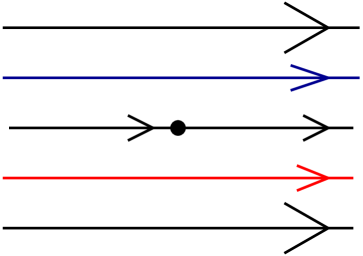
Figure 2. Kocergin Flow is topologically equivalent to the area preserving flow shown on Figure 1 with separatrix loop removed. The rest point is responsible for the shear along the orbits.

If one is interested in flows with singularities preserving a finite non-atomic measure then the simplest example can be obtained by plugging (by smooth surgery) in the phase space of the minimal two dimensional linear flow an isolated singularity coming from a Hamiltonian flow in $\mathbb{R}^{2}$ (see Figure 2). The so called Kochergin flows thus obtained preserve besides the Dirac measure at the singularity a measure that is equivalent to Lebesgue measure [71]. As it was explained in Section 2 Kochergin flows model smooth area preserving flows on $\mathbb{T}^{2}.$ These flows still have $\mathbb{T}$ as a global section with a minimal rotation for the return map, but the slowing down near the fixed point produces a singularity for the return time function above the last point where the section intersects the incoming separatrix of the fixed point. The strength of the singularity depends on how abruptly the linear flow is slowed down in the neighborhood of the fixed point. A mild slowing down, or mild shear, is typically represented by the logarithm while stronger singularities such as $x^{-a},a\in(0,1)$ are also possible. Powerlike singularities appear naturally in the study of area preserving flows with degenerate fixed points. We shall see below that dynamical properties of the special flows are quite different for logarithmic and power like singularities.

Question 41.

What can be said about the deviations of the ergodic sums above Kocergin flows?

8.4. Mixing properties.

We give first a classical criterion for weak mixing of special flows. Its proof is similar to the proof of the ergodicity criterion for skew products given by Proposition 4.

Proposition 6.

([126]) $T_{\alpha,A}$ is weak mixing iff for any $\lambda\in\mathbb{R}^{*}$, there are no measurable solutions to the multiplicative cohomological equation

(38) $$e^{i2\pi\lambda A(x)}=\psi(x+\alpha)/\psi(x).$$

Indeed if $h(x,t)$ is the eigenfunction when for almost all $x$ the function $h(x,t)e^{-\lambda t}$ takes the same value $\psi(x)$ for almost almost all $t.$ Then (38) follows from the identification (34).

Theorem 42.

([35]) If the vector $\alpha\in{\mathbb{R}}^{d}$ is not $\beta$-Diophantine then there exists a dense $G_{\delta}$ for the $C^{\beta+d}$ topology, of functions $\varphi\in C^{\beta+d}({\mathbb{T}}^{d},{\mathbb{R}}^{*}_{+}),$ such that the special flow constructed over $T_{\alpha}$ with the ceiling function $\varphi$ is weak mixing.

This result is optimal since smooth time changes of linear flows with Diophantine vectors $\alpha,$ are smoothly conjugated to the linear flow and, hence, are not weak mixing.

Mixing of special flows is more delicate to establish since one needs to have uniform distribution on increasingly large scales in $\mathbb{R}^{+}$ of the sums $A_{N}$ for all integers $N\to\infty$, and this above arbitrarily small sets of the base space. Indeed mixing of special flows above non mixing base dynamics is in general proved as follows: if the ergodic sums $A_{N}$ become as $N\to\infty$ uniformly stretched (well distributed inside large intervals of $\mathbb{R}_{+}$) above small sets, the image by the special flow at a large time $T$ of these small sets decomposes into long strips that are well distributed in the fibers due to uniform stretch and well distributed in projection on the base because of ergodicity of the base dynamics (see Figure 3).

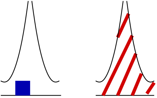
Figure 3. Mixing mechanism for special flows: the image of a rectangle is a union of long narrow strips which fill densely the phase space.

The delicate point however is to have uniform stretch for all integers $N\to\infty$. In particular the following result has been essentially proven in [70].

Theorem 43.

If $A$ has DKP then $T_{\alpha,A}^{t}$ is not mixing.

Proof.

If $A$ has the DKP then there is a set $\Omega$ of positive measure on which (30) holds for positive density of $n_{k}.$ By passing to a subsequence we can find a set $I$ of positive measure, a sequence $\{t_{k}\}$ and a vector $\beta$ such that on $\Omega$ $|A_{n_{k}}-t_{k}|<C$ and $\alpha n_{k}\to\beta.$ Pick a small $\eta.$

$$\Omega_{i}=\cup_{0\leq t\leq\eta}T_{\alpha,A}^{t}[I\times\{0\}],\quad\Omega_{f}=\cup_{0\leq|t|\leq C+\eta}T_{\alpha,A}^{t}[(I+\beta)\times\{0\}].$$

By decreasing $I$ if necessary we obtain that those sets have measures strictly between $0$ and $1.$ On the other hand it is not difficult to see from the definition of the special flow that $\mu(T_{\alpha,A}^{t_{k}}\Omega_{i}\cap\Omega_{f})\to\mu(\Omega_{i})$ contradicting the mixing property. ∎

In particular the flows with ceiling functions $A$ of bounded variation or functions with symmetric log singularities are not mixing.

In fact, since the sDKP holds for any minimal circle diffeomorphism, it follows from (35) and (37) that any smooth flow on $\mathbb{T}^{2}$ without cycles or fixed points is not topologically mixing. We leave this as an exercise for the reader.

The first positive result about mixing of special flows is obtained in [71].

Theorem 44.

If $\alpha\in\mathbb{R}-\mathbb{Q}$ and $A$ has (integrable) power singularities then $T_{\alpha,A}$ is mixing.

The reason why the case of power singularities is easier than the logarithmic case (corresponding to non-degenerate flows on $\mathbb{T}^{2}$) is the following. The standard approach for obtaining the stretching of ergodic sums is to control $\frac{\partial A_{n}}{\partial x}=\left(\frac{\partial A}{\partial x}\right)_{n}$ For $A$ as in theorem 44, $\frac{\partial A}{\partial x}$ has singularities of the type $x^{-a}$ with $a>1.$ In this case the main contribution to ergodic sums comes from the closest encounter with the singularity (cf. Theorem 3) making the control of the stretch easier. Moreover, the strength of the singularity allows to obtain speed of mixing estimates.

Theorem 45.

([34]) If $\alpha$ is Diophantine and $A$ has a (integrable) power singularity then $T_{\alpha,A}^{t}$ is power mixing.

More precisely, there exists a constant $\beta=\beta(\alpha)$ such that if $R_{1},R_{2}$ are rectangles in $\mathbb{T}\times\mathbb{R}$ then

(39) $$\left|\mu(R_{1}\cap T^{t}R_{2})-\mu(R_{1})\mu(R_{2})\right|\leq Ct^{-\beta}.$$

The exponent $\beta$ in [34] seems to be non optimal.

Question 42.

For $\alpha$ Diophantine find the asymptotics of the LHS of (39).

It is interesting to surpass the threshold $\beta=1/2$. In particular, one would like to answer the following question.

Question 43.

[83] Can a smooth area preserving flow on $\mathbb{T}^{2}$ have Lebesgue spectrum?

On the other hand for logarithmic singularities there might be cancelations in ergodic sums of $\frac{\partial A}{\partial x},$ making the question of mixing more tricky.

Theorem 46.

Let $A$ be as in Question 1.

(a) ([72]) If $\sum_{j}a_{j}^{+}=\sum_{j}a_{j}^{-}$ then $T_{\alpha,A}^{t}$ is not mixing for any $\alpha\in\mathbb{R}-\mathbb{Q}.$

(b) ([119, 73]) If $\sum_{j}a_{j}^{+}\neq\sum_{j}a_{j}^{-}$ then $T_{\alpha,A}^{t}$ is mixing for almost every $\alpha\in\mathbb{R}-\mathbb{Q}.$

(c) ([73]) If $a_{j}^{+}-a_{j}^{-}$ has the same sign for all $j$ then $T_{\alpha,A}^{t}$ is mixing for each $\alpha\in\mathbb{R}-\mathbb{Q}.$

Question 44.

([74]) Does the condition that $\sum_{j}a_{j}^{+}\neq\sum_{j}a_{j}^{-}$ imply $T_{\alpha,A}^{t}$ is mixing for every $\alpha\in\mathbb{R}-\mathbb{Q}$?

Question 45.

([74]) Under the conditions of Theorems 44 and 46 is $T_{\alpha,A}^{t}$ mixing of all orders?

In higher dimensions much less is known. Note that for smooth ceiling functions Theorems 30, 39 and 43 precludes mixing for a set of rotation vectors of full measure that also contains a residual set.

The following was shown in [36]. Recall the definition of the set $Y$ used in Theorem 31. Define the following real analytic complex valued function on ${\mathbb{T}}^{2}$:

$${\mathcal{A}}(x,y)=\left(\sum_{k=2}^{\infty}{e^{i2\pi kx}\over e^{k}}+\sum_{k=2}^{\infty}{e^{i2\pi ky}\over e^{k}}\right).$$

Theorem 47.

For any $(\alpha^{\prime},\alpha^{\prime\prime})\in Y$, the special flow constructed over the translation $T_{\alpha^{\prime},\alpha^{\prime\prime}}$ on ${\mathbb{T}}^{2}$, with the ceiling function $1+\mathrm{Re}{\mathcal{A}}$ is mixing.

Because of the disposition of the best approximations of $\alpha^{\prime}$ and $\alpha^{\prime\prime}$ the ergodic sums $\varphi_{m}$ of the function $\varphi$, for any $m$ sufficiently large, will be always stretching (i.e. have big derivatives), in one or in the other of the two directions, $x$ or $y$, depending on whether $m$ is far from $\{q^{\prime}_{n}\}$ or far from $\{q^{\prime\prime}_{n}\}$. And this stretch will increase when $m$ goes to infinity. So when time goes from $0$ to $t$, $t$ large, the image of a small typical interval $J$ from the basis ${\mathbb{T}}^{2}$ (depending on $t$ the intervals should be taken along the $x$ or the $y$ axis) will be more and more distorted and stretched in the fibers’ direction, until the image of $J$ at time $t$ will consist of a lot of almost vertical curves whose projection on the basis lies along a piece of a trajectory under the translation $T_{\alpha^{\prime},\alpha^{\prime\prime}}$. By unique ergodicity these projections become more and more uniformly distributed, and so will $T^{t}(J)$. For each $t$, and except for increasingly small subsets of it (as function of $t$), we will be able to cover the basis with such “typical” intervals. Besides, what is true for $J$ on the basis is true for $T^{s}(J)$ at any height $s$ on the fibers. So applying Fubini Theorem in two directions, first along the other direction on the basis (for a time $t$ all typical intervals are in the same direction), and second along the fibers, we will obtain the asymptotic uniform distribution of any measurable subset, which is, by definition, the mixing property.

Question 46.

Are the flows obtained in Theorem 47 mixing of all orders?

Question 47.

For which vectors $\alpha\in\mathbb{R}^{d}$, there exist special flows above $T_{\alpha}$ with smooth functions $A$ such that $T^{t}_{\alpha,A}$ is mixing?

The foregoing discussion demonstrates that both ergodicity of cylindrical cascades and mixing of special flows require a detailed analysis of ergodic sums (1). However, the estimates needed in those two cases are quite different and somewhat conflicting. Namely, for ergodicity we need to bound from below the probability that ergodic sums hit certain intervals, while for mixing one needs to rule out too much concentration. For this reason it is difficult to construct functions $A$ such that $W_{\alpha,A}$ is ergodic while $T_{\alpha,c+A}^{t}$ is mixing. In fact, so far this has only been achieved for smooth functions with asymmetric logarithmic singularities. However, it seems that in higher dimensions there is more flexibility so such examples should be more common.

Question 48.

Is it true that for (almost) every polyhedron $\Omega\in\mathbb{T}^{d}$, $d\geq 2$, and almost every $a>0$, and almost every $\alpha\in\mathbb{T}^{d}$, the special flow above $\alpha$ and under the function $a+\chi_{\Omega}$ is mixing?

Note that a positive answer to both this question and Question 35 will give a large class of interesting examples where ergodicity of $W_{\alpha,A}$ and mixing for $T_{\alpha,c+A}$ (for any $c$ such that $c+A>0$) hold simultaneously.

Question 49.

Answer Questions 35 and 48 in the case $\Omega$ is a strictly convex analytic set.

8.5. An application.

Here we show how the geometry of special flows above cylindrical cascades can be used to study the ergodic sums.

Proof of Theorem 38..

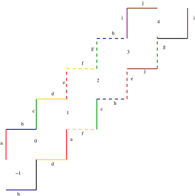
Figure 4. Staircase surfaces. The sides marked by the same symbol are identified.

The proof uses the properties of the staircase surface $St$ shown on Figure 4. The staircase is an infinite pile of $2\times 1$ rectangles so that the left bottom corner of the next rectangle is attached to the center of the top of the previous one. The sides which are differ by two units in either horizontal or vertical direction are identified. We number all the rectangles from $-\infty$ to $+\infty$ as shown on Figure 4. There is a translational symmetry given by $G(x,y)=(x+1,y+1)$ and $St/G$ is a torus. We shall use coordinates $\bar{p}=(p,z)$ on the staircase where $p$ are coordinates on the torus which is the identified with rectangle zero and $z\in\mathbb{Z}$ is the index of rectangle. Thus we have $(p,z)=G^{z}(p,0).$

The key step in the proof is an observation of [53] that $St$ is a Veech surface. Namely, given $A\in SL_{2}({\mathbb{Z}})$ such that $A\equiv I\mod 2$ there exists unique automorphism $\phi_{A}$ of $St$ which commutes with $G,$ fixes the singularities of $St,$ has derivative $A$ at the non-singular points and has drift $0.$ That is, in our coordinates

(40) $$\phi(p,z)=(Ap,z+\tau(p))$$

and the drift condition means that $\int_{\mathbb{T}^{2}}\tau(p)dp=0.$

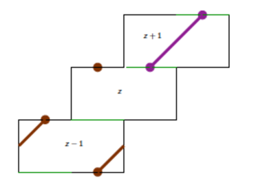
Figure 5. Poincare map for a linear flow on the staircase. Orbits starting from $[1/2,1]$ go up while orbits starting from $[0,1/2)$ have to go down due to the gluing conditions.

Consider the linear flow on $St$ with slope $\theta$ which is locally given by $T^{t}(x,y)=(x+t\cos\theta,y+t\sin\theta).$ Let $\Pi$ be the union of the top sides of the rectangles in $St.$ We identify $\Pi$ with $\mathbb{T}\times\mathbb{Z}$ using the map $\eta:\mathbb{T}\times\mathbb{Z}\to\Pi$ such that $\eta(x,z)$ is the point on the top side of rectangle $z$ at the distance $2x$ from the left corner. It is easy to check (see Figure 5) that under this identification the Poincare map for $T^{t}$ takes form

$$(x,z)=(x+\alpha,z+\chi_{[1/2,1]}(x)-\chi_{[0,1/2)}(z))\text{ where }\alpha=\frac{\tan\theta+1}{2}.$$

Now suppose that $\alpha$ and hence $\tan\theta$ is a quadratic surd. By Lagrange theorem there is $A\in SL_{2}({\mathbb{Z}})$ such that $A\left(\begin{array}[]{c}\cos\theta\\ \sin\theta\end{array}\right)=\lambda\left(\begin{array}[]{c}\cos\theta\\ \sin\theta\end{array}\right).$ By replacing $A$ by $A^{k}$ for a suitable (positive or negative) $k$ we may assume that $A\equiv I\mod 2$ and that $\lambda<1.$ Let $\Gamma_{N}(x)$ be the ray starting from $\eta(x,0)$ having slope $\theta$ and length $\frac{N}{\sin\theta}.$

$${\mathbb{L}}_{N}=\frac{{\rm mes}(\bar{p}\in\Gamma_{N}(x):z(\bar{p})=0)}{{\text{length}}(\Gamma_{N}(x)}=\frac{{\rm mes}(\bar{q}\in{\tilde{\Gamma}}(x):z(\phi_{A}^{-m})=0)}{{\text{length}}({\tilde{\Gamma}})}$$

$$={\mathbb{P}}_{x}(z(\phi_{A}^{-m}\bar{q})=0)$$

where $\tilde{\Gamma}=\phi_{A}^{m}\Gamma_{N}(x)$ and ${\mathbb{P}}_{x}$ is computed under the assumption that $\bar{q}$ is uniformly distributed on ${\tilde{\Gamma}}.$ Choose $m$ to be the smallest number such that ${\text{length}}(\phi^{m}_{A}\Gamma_{N}(x))=\lambda^{m}\frac{N}{\sin\theta}\leq 1.$ Note that $m\approx\frac{\ln N}{\ln\lambda}.$ By our choice of $m,$ ${\tilde{\Gamma}}$ is either contained in a single rectangle or intersects two of them. Let us consider the first case, the second one is similar. So we assume that ${\tilde{\Gamma}}$ is in the rectangle with index $a$ so that $\bar{q}=(q,a).$ Due to (40) $z(\phi^{-m}\bar{q})=a-\sum_{j=1}^{m}\tau(\phi_{A}^{-j}q).$ Thus

$${\mathbb{P}}_{x}\left(z(\phi_{A}^{-m}\bar{q})=0\right)={\mathbb{P}}_{x}\left(\sum_{j=1}^{m}\tau(\phi_{A}^{-j}q=a)\right).$$

Now we apply the Local Limit Theorem for linear toral automorphisms (see [101, Section 4] or [46]) which says that there is a constant $\sigma^{2}$

$${\mathbb{P}}_{x}\left(\sum_{j=1}^{n}\tau(\phi_{A}^{-j}q)\right)\approx\frac{1}{\sqrt{2\pi m}\sigma}e^{-a^{2}/2\sigma^{2}m}.$$

It remains to note that

$$a(x)=\sum_{j=0}^{m-1}\tau(\phi_{A}^{j}\eta(x,0))$$

so applying the Central Limit Theorem for linear toral automorphisms we see that if $x$ is uniformly distributed on $\mathbb{T}^{1}$ then $\frac{a(x)}{\sqrt{m}}$ is approximately normal with zero mean and variance $\sigma^{2}.$ ∎

Next we discuss the proof of Theorem 8(b) in case $l=\frac{1}{2}.$ The proof proceeds the same way as the proof of Theorem 38 with the following changes.

(I) Instead of estimating the probability that $z(\phi^{-m}_{A}\bar{q})=0$ we need to estimate the probability that $z(\phi^{-m}_{A}\bar{q})$ belongs to an interval of length $\sqrt{m}$ so we use the Central Limit Theorem instead of the Local Limit Theorem.

(II) Instead of taking $x$ random we take $x$ fixed at the origin. Note that the origin is fixed by $A$ so $\tau(\phi^{m}_{A}(0,0))=Cm.$ (More precisely $\tau$ is multivalued at the origin since it belong to several rectangles so by $\tau(\phi^{m}_{A}(0,0))$ we mean the limit of $\tau(\phi^{m}_{A}(\bar{p}))$ as $\bar{p}$ approaches the origin inside $\Gamma_{N}(0).$)

9. Higher dimensional actions

Question 50.

Generalize the results presented in Sections 2-8 to higher dimensional actions.

The orbits of commuting shifts $T^{n}x=x+\sum_{j=1}^{q}n_{j}\alpha_{j}$ are much less studied than their one-dimensional counterparts. We expect that some of the results of Sections 2-8 admit straightforward extensions while in other cases significant new ideas will be necessary. Below we discuss two areas of research where multidimensional actions appear naturally.

9.1. Linear forms.

Statements about orbits of a single translation can be interpreted as results about joint distribution of fractional part of inhomogenuous linear forms of one variable evaluated over $\mathbb{Z}$. From the point of view of Number Theory it is natural to study linear forms of several variables evaluated over $\mathbb{Z}^{d}$. Let

$$l_{i}(n)=x_{i}+\sum_{j=1}^{q}\alpha_{ij}n_{j},\quad i=1\dots d.$$

Thus it is of interest to study the discrepancy

$$\mathbb{D}_{N}(\Omega,\alpha,x)=\\ {\mathrm{Card}}(0\leq n_{j}<N,j=1,\ldots,q:(\{l_{1}(n)\},\dots\{l_{d}(n)\})\in\Omega)-N^{q}\text{Vol}(\Omega).$$

The latter problem is a classical subject in Number Theory, and there are several important results related to it. In particular, the Poisson regime is well understood ([88]). The following result generalizes Theorem 16 and can be proven by a similar argument.

Theorem 48.

Let $(\alpha,x)$ be uniformly distributed on $\mathbb{T}^{d(q+1)}.$ Then, for any cube $\Sigma\subset\mathbb{R}^{q}$, the distribution of

$${\mathrm{Card}}(n:\frac{n}{N}\in\Sigma\text{ and }(\{l_{1}(n)\},\dots\{l_{d}(n)\})\in N^{-q/d}\Omega)$$

converges as $N\to\infty$ to

$${\mathcal{N}}(\Omega,\Sigma):={\mathrm{Card}}(e\in L,e=(x,y):x(e)\in\Omega,y(e)\in\Sigma)$$

where $L$ is a random affine lattice in $\mathbb{R}^{d+q}.$

Thus the Poisson regime for the rotations exhibits more regular behavior comparing to standard Poisson processes. However then the number of rotations becomes large the limiting distribution approaches the Poisson. Namely, the following is the special case of the result proven in [125].

Theorem 49.

If $\Sigma_{q}$ are unit cubes in $\mathbb{R}^{q}$ then $\Omega\to{\mathcal{N}}(\Omega,\Sigma_{q})$ converges as $q\to\infty$ to the Poisson measure ${\boldsymbol{\mu}}(\Omega)={\mathrm{Card}}(\mathfrak{P}\cap\Omega)$ where $\mathfrak{P}$ is a Poisson process on $\mathbb{R}^{d}$ with constant intensity.

Next we present extensions of Theorems 25, 24, 26 and 27 to the context of homogeneous and inhomogeneous linear forms. Let again $l_{i}(n)=x_{i}+\sum_{j=1}^{q}\alpha_{ij}n_{j},$ $i=1\dots d.$ Consider

$$V_{N}(\alpha,x,c)={\mathrm{Card}}(0\leq n_{i}<N:(\{l_{1}(n)\},\dots\{l_{d}(n)\})\in B(c|n|^{-q/d})).$$

More generally given a function $\psi:{\mathbb{R}}^{+}\to{\mathbb{R}}^{+}$ define

$$V^{\psi}_{N}(\alpha,x)={\mathrm{Card}}(0\leq n_{i}<N:(\{l_{1}(n)\},\dots\{l_{d}(n)\})\in B(\psi(|q|)).$$

We also let $U_{N}(\alpha,c)=V_{N}(0,\alpha,c)$ and $U_{N}^{\psi}(\alpha)=V_{N}^{\psi}(0,\alpha)$ be the quantities measuring the rate of recurrence.

In particular we call the matrix $\alpha$ badly approximable if there exists $c>0$ such that for, $V_{N}(0,\alpha,c)$ is bounded. On the other hand, if $U_{N}^{\psi}(\alpha)\to\infty$ where $\psi(r)=r^{-(d/q+{\varepsilon})}$ then $\alpha$ is called very well approximable (VWA).

The following result is known as Khinchine–Groshev Theorem. Almost sure is considered relative to Lebesgue measure on the space of matrices $\alpha\in\mathbb{T}^{dq}$.

Theorem 50.

[64, 47, 31, 116, 14, 7] (a) If $\sum_{\mathbb{Z}^{q}}|\psi^{d}(|n|)<\infty$ then $U_{N}^{\psi}$ is bounded almost surely.

(b) If $\sum_{\mathbb{Z}^{q}}\psi^{d}(|n|)=+\infty$ and either $\psi$ is decreasing or $dq>1$ then $\lim_{N\to\infty}U_{N}^{\psi}(\alpha)=+\infty$ almost surely.

(c) For $d=q=1$ there exists $\psi$ such that $\sum_{n\in Z}\psi(|n|)=+\infty$ but $U_{N}^{\psi}$ is bounded almost surely.

(d) If $\psi$ is decreasing and $\sum_{n\in Z^{d}}\psi^{d}(|n|)=+\infty$ then $V_{N}^{\psi}(\alpha,x)\to\infty$ almost surely.

In particular, both badly approximable and very well approximable $\alpha$s have zero measure.

When the number of hits is infinite, it is natural to consider the question of the sBC property.

Theorem 51.

[116] (a) For almost all $\alpha$

$$U_{N}^{\psi}(\alpha)={\mathbb{E}}(U_{N}^{\psi})+O\left(\sqrt{\Gamma(N)\ln^{3}\Gamma(N)}\right)$$

where

$$\Gamma(N)=\sum_{|n|\leq N}\psi(|n|)^{d}D(gcd(n_{1}\dots n_{q}))$$

and $D$ denotes the number of divisors.

(b) $\Gamma(N)\leq C{\mathbb{E}}(U_{N}^{\psi})$ if either $q>3$ or $q=2$ and $n\psi^{2}(n)$ is decreasing.

(c) If $q=1$ and $\psi(n)$ is decreasing then for each $\delta$

$$U_{N}^{\psi}(\alpha)={\mathbb{E}}(U_{N}^{\psi})+O\left(\sqrt{{\tilde{\Gamma}}(N){\mathbb{E}}(U_{N}^{\psi})}\ln^{2+\delta}({\mathbb{E}}(U_{N}^{\psi}))\right)$$

where

$${\tilde{\Gamma}}(N)=\sum_{n=1}^{N}\frac{\psi(n)}{n}.$$

Question 51.

Does a similar formula as that of Theorem 51 hold for $V^{\psi}$?

Some partial results are obtained in [117].

It follows from the same arguments as the proof of Theorem 24 sketched in Section 6.3 that the sBC property holds for $\psi(r)=r^{-(d/q)}$ for almost every $(\alpha,x)$, that is

$$\lim_{N\to\infty}\frac{V_{N}(\alpha,x)}{{\mathbb{E}}(V_{N}(\alpha,x))}=1.$$

For badly approximable $\alpha$ we have the following.

Theorem 52.

[90] Let $x$ be uniformly distributed on $\mathbb{T}^{d}.$ If $\alpha$ is badly approximable, there exists a constant $K$ such that all limit points of $\frac{V_{N}-{\mathbb{E}}(V_{N})}{\sqrt{\ln N}}$ are normal random variables with zero mean and variance $\sigma^{2}$ where $0\leq\sigma^{2}\leq K.$

Question 52.

(a) Show that there exist a constant $\bar{\sigma}^{2}>0$ such that for almost all $\alpha$ $\dfrac{V_{N}-{\mathbb{E}}(V_{N})}{\sqrt{\ln N}}$ converges to ${\mathfrak{N}}(\bar{\sigma}^{2}).$

(b) Does there exist $\alpha$ such that $\lim\inf_{N\to\infty}\dfrac{V_{N}-{\mathbb{E}}(V_{N})}{\sqrt{\ln N}}=0$ (that is, $\sqrt{\ln N}$ is not a correct normalization for such $\alpha$)?

For random $\alpha$ we have the following.

Theorem 53.

([30]) There exists $\sigma$ such that If $\alpha_{1},\ldots,\alpha_{r}$ and $x_{1},\ldots,x_{d}$ are randomly distributed on $\mathbb{T}^{dr+d}$ then $\frac{V_{N}-{\mathbb{E}}(V_{N})}{\sqrt{\ln N}}$ converges in distribution to a normal random variables with zero mean and variance $\sigma^{2}$. A similar convergence holds if $d+r>2$, $(x_{1},\ldots,x_{r})=(0,\ldots,0)$ and only the $\alpha_{i}$’s are random.

Still there are many open questions. We provide several examples.

Question 53.

Extend Theorems 10 and 11 to the case $q>1.$

We note that in the case of Theorem 11, even the case $d=1$ seems quite difficult. One can attack this question using the method of [29] but it runs into the problem of lack of parameters described after Question 24.

Question 54.

Let $l,{\hat{l}}:\mathbb{R}^{d}\to\mathbb{R},$ be linear forms with random coefficients, $Q:\mathbb{R}^{d}\to\mathbb{R}$ be a positive definite quadratic form. Investigate limit theorems, after adequate renormalization, for the number of solutions to

(a) $\{l(n)\}Q(n)\leq c,|n|\leq N;$

(b) $\{l(n)\}|{\hat{l}}(n)|\leq c,|n|\leq N;$

(c) $|l(n)Q(n)|\leq c,|n|\leq N;$

(d) $|l(n){\hat{l}}(n)|<c,|n|\leq N.$

While (a) and (b) have obvious interpretation as shrinking target problems for toral translations, such interpretation for (c) and (d) is less straightforward. Consider for example (c). Let $l(n)=\sum_{j=1}^{q}\alpha_{j}n_{j}.$ Dividing the distribution of $\alpha$ into thin slices we may assume that $\alpha_{d}$ is almost constant. If $\alpha_{d}\approx a$ then we can compare our problem with $|\left(\sum_{j=1}^{q-1}{\tilde{\alpha}}_{j}n_{j}\right)+n_{q}|Q(n)<{\tilde{c}}$ where ${\tilde{\alpha}}_{j}=\alpha_{j}/a,{\tilde{c}}=c/a.$ Since $|l(n)|$ should be small we must have $|\left(\sum_{j=1}^{q-1}{\tilde{\alpha}}_{j}n_{j}\right)+n_{q}|=\{\sum_{j=1}^{q}{\tilde{\alpha}}_{j}\}$ in which case $Q(n_{1},\dots,n_{q-1},n_{q})$ is well approximated by

$$Q(n_{1},\dots,n_{q-1},-\sum_{j=1}^{q-1}{\tilde{\alpha}}_{j}n_{j})$$

so we have a shrinking target problem in lower dimensions. In fact as we saw in Section 5 typically the proof proceeds in the opposite direction by getting rid of fractional part at the expense of increasing dimension since problems (c) and (d) have more symmetry and so should be easier to analyze.

We note that part (d) deals with degenerate quadratic form. The case of non-degenerate forms is discussed in [32, Sections 5 and 6].

9.2. Cut-and-project sets.

Cut-and-project sets are used in physics literature to model quasicrystals. To define them we need the following data: a lattice in $\mathbb{R}^{d},$ a decomposition $\mathbb{R}^{d}=E_{1}\oplus E_{2}$ and a compact set (a window) ${\mathcal{W}}\subset E_{2}.$ Let $P_{1}$ and $P_{2}$ be the projections to $E_{1}$ and $E_{2}$ respectively. The cut-and-project set is defined by

$${\mathcal{P}}=\{P_{1}(e),e\in L\text{ and }P_{2}(e)\in{\mathcal{W}}\}.$$

We suppose in the following discussion that

$$\overline{E_{1}+L}=\mathbb{R}^{d}\text{ and }L\cap E_{2}=\emptyset.$$

Then ${\mathcal{P}}$ is a discrete subset of $E_{1}$ sharing many properties of lattices but having a more complicated structure. Note that the limiting distributions in Theorems 16 and 48 are described in terms of cut-and-project sets. We refer the reader to [93, Sections 16 and 17] for more discussion of cut-and-project set. Here we only mention the fact that such sets have asymptotic density. Let ${\mathcal{P}}_{R}=\{t\in{\mathcal{P}}:|t|\leq R\}.$

Theorem 54.

Suppose that ${\mathcal{W}}$ is an open subset of $E_{2}$ with a piecewise smooth boundary. Then

$$\lim_{R\to\infty}\frac{{\mathrm{Card}}({\mathcal{P}}_{R})}{{\mathrm{Vol}}(B(0,R))}=\frac{{\mathrm{Vol}}({\mathcal{W}})}{\mathrm{covol}(L)}\frac{{\mathrm{Vol}}_{\mathbb{R}^{d}}}{{\mathrm{Vol}}_{E_{1}}{\mathrm{Vol}}_{E_{2}}}.$$

Proof.

(Following [52]). Note that $t\in{\mathcal{P}}$ iff there exists $e\in L$ such that $-t+e\in{\mathcal{W}},$ that is $-t\in{\mathcal{W}}\text{ mod }L.$ Consider the action of $E_{1}$ on $\mathbb{R}^{d}/L$ given by $T^{t}(x)=x+t.$ Then ${\mathcal{P}}_{R}$ counts the number of intersections of the orbit of the origin of size $R$ with ${\mathcal{W}}.$ Pick a small $\delta$ and let ${\mathcal{W}}_{\delta}=\{{\mathcal{W}}+t,|t|\leq\delta\}.$ Then ${\mathcal{W}}_{\delta}$ is a subset of $\mathbb{R}^{d}/L$ and for small $\delta$

(41) $${\mathrm{Vol}}({\mathcal{W}}_{\delta})={\mathrm{Vol}}({\mathcal{W}}){\mathrm{Vol}}(B(0,\delta))\dfrac{{\mathrm{Vol}}_{\mathbb{R}^{d}}}{{\mathrm{Vol}}_{E_{1}}{\mathrm{Vol}}_{E_{2}}}.$$

Next,

(42) $$\int_{|t|<R}\chi_{{\mathcal{W}}_{\delta}}(T^{t}0)dt={\mathrm{Vol}}(B(0,\delta)){\mathrm{Card}}({\mathcal{P}}_{R})+O(R^{q-1})$$

where $q=\dim(E_{1})$ and the second term represents boundary contribution. On the other hand by unique ergodicity of $T^{t}$

(43) $$\int_{|t|<R}\chi_{{\mathcal{W}}_{\delta}}(T^{t}0)dt={\mathrm{Vol}}(B(0,R))\frac{{\mathrm{Vol}}({\mathcal{W}}_{\delta})}{\mathrm{covol}(L)}+o(R^{q}).$$

Combining (41), (42) and (43) we get the result. ∎

Question 55.

Describe the error term in the asymptotics of Theorem 54.

If $q=1$ then the error term in (42) is negligible and so (42) can be used to describe the deviations (see [28] for the case where ${\mathcal{W}}$ is convex). If $q>1$ more work is needed to control both the LHS and the RHS of (42).

While the methods of [28, 29] deal with the case where $\dim(E_{1})$ is as small as possible, the most classical case is the opposite one when $\dim(E_{2})$ is as large as possible, that is, studying lattice points in large regions. Here we can not attempt to survey this enormous topic, so we refer the reader to the specialized literature on the subject ([56, 57, 77]. We just mention that limit theorems similar in spirit to the results discussed in this paper are obtained in [49, 16, 17, 104]. More generally, instead of considering large balls one can count the number of lattice points in $RD$ where $D$ is a fixed regular set. As in Section 2 the order of the error term is sensitive to the geometry of $D$ (see e.g. [15, 78, 86, 96, 105, 109, 110, 121, 122] and references wherein). In fact, one can also consider the varying shapes $RD_{R}$ which includes both the Poisson regime where ${\mathrm{Vol}}(RD_{R})$ does not grow (see [18] and references wherein) and the intermediate regime where ${\mathrm{Vol}}(RD_{R})$ grows but at the rate slower than $R^{d}$ (see [54, 127]).

This motivates the following question

Question 56.

Extend the results of the above mentioned papers to cut-and-project sets.

References

- [1] Aaronson J. An Introduction to Infinite Ergodic Theory, Math. Surveys and Monographs 50, Amer. Math. Soc. 1997.
- [2] Aaronson J., Keane M. The visits to zero of some deterministic random walks, Proc. London Math. Soc. 44 (1982) 535–553.
- [3] Arnold V. I. Topological and ergodic properties of closed -forms with incommensurable periods, Funkts. Anal. Prilozhen. 25 (1991) 1–12.
- [4] Athreya J. Logarithm laws and shrinking target properties, Proceedings–Math. Sciences 119 (2009) 541–557.
- [5] Atkinson G. Recurrence of co-cycles and random walks, J. London Math. Soc. 13 (1976) 486–488.
- [6] Avila A., Dolgopyat D., Duriev E., Sarig O. The visits to zero of a random walk driven by an irrational rotation, to appear in Israel Math. J.
- [7] Badziahin D., Beresnevich V., Velani S. Inhomogeneous theory of dual Diophantine approximation on manifolds, Adv. Math. 232 (2013) 1–35.
- [8] Beck J. Probabilistic Diophantine approximation. I. Kronecker sequences, Ann. of Math. 140 (1994) 449–502.
- [9] Beck J., Diophantine approximation and quadratic fields in Number theory (Eger, 1996), (edited by K. Gyory, A. Petho, V. T. Sos) de Gruyter, Berlin, 1998, pp. 55–93.
- [10] Beck J., From probabilistic Diophantine approximation to quadratic fields, Random and quasi-random point sets, 1 48, Springer Lecture Notes in Statist., 138 (1997) 1–48.
- [11] Beck J., Randomness of the square root of 2 and the giant leap, Period. Math. Hungar. Part I: 60 (2010) 137–242; Part II: 62 (2011) 127–246.
- [12] Bekka M. B., Mayer M. Ergodic theory and topological dynamics of group actions on homogeneous spaces,London Math. Soc. Lect. Note Ser. 269 Cambridge University Press, Cambridge, 2000. x+200 pp.
- [13] V. Beresnevich, V. Bernik, D. Kleinbock, G. A. Margulis, Metric Diophantine approximation: The Khintchine–Groshev theorem for non-degenerate manifolds, Moscow Math. J. 2 (2002), 203–225.
- [14] Beresnevich V., Velani S. Classical metric Diophantine approximation revisited: the Khintchine-Groshev theorem, IMRN (2010) no. 1, 69–86.
- [15] Bleher P. On the distribution of the number of lattice points inside a family of convex ovals, Duke Math. J. 67 (1992) 461–481.
- [16] Bleher P., Bourgain, J. Distribution of the error term for the number of lattice points inside a shifted ball, Progr. Math. 138 (1996) 141–153 Birkhauser Boston.
- [17] Bleher P. M., Cheng Z., Dyson F. J., Lebowitz J. L. Distribution of the error term for the number of lattice points inside a shifted circle, Comm. Math. Phys. 154 (1993) 433–469.
- [18] Bleher P. M., Lebowitz J. L. Variance of number of lattice points in random narrow elliptic strip, Ann. Inst. H. Poincare Probab. Statist. 31 (1995) 27–58.
- [19] J. W. S. Cassels, An introduction to Diophantine approximation, Cambridge Tracts in Math., vol. 45, Cambridge Univ. Press, Cambridge, 1957.
- [20] Chaika J, Constantine D. Quantitative Shrinking Target Properties for rotations, interval exchanges and billiards in rational polygons, arXiv preprint 1201.0941.
- [21] Chernov N., Kleinbock D. Dynamical Borel-Cantelli lemmas for Gibbs measures, Israel J. Math. 122 (2001) 1–27.
- [22] Chevallier N., Conze J.–P. Examples of recurrent or transient stationary walks in over a rotation of Contemp. Math 485 (2009) 71–84.
- [23] Conze J.-P., Recurrence, ergodicity and invariant measures. for cocycles over a rotation, Contemp. Math. 485 (2009) 45–70.
- [24] Conze J.-P., Keane, M. Ergodicité d’un flot cylindrique, Seminaire de Prob.-I, Univ. Rennes, Rennes, 1976, Exp. No. 5, 7 pp.
- [25] Conze J.-P., Piekniewska A., On multiple ergodicity of affine cocycles over irrational rotations, arXiv:1209.3798
- [26] de Simoi J., Liverani C. The martingale approach after Varadhan and Dolgopyat, this volume.
- [27] Dolgopyat D. Limit theorems for partially hyperbolic systems, Trans. AMS 356 (2004) 1637–1689.
- [28] Dolgopyat D., Fayad B. Deviations of ergodic sums for toral translation-I: Convex bodies, GAFA 24 (2014) 85–115.
- [29] Dolgopyat D., Fayad B. Deviations of ergodic sums for toral translations-II: Boxes, arXiv preprint 1211.4323.
- [30] Dolgopyat D., Fayad B., Vinogradov I., Central limit theorems for simultaneous Diophantine approximations, in preparation.
- [31] Duffin R. J., Schaeffer A.C. Khintchine’s problem in metric Diophantine approximation, Duke Math. J. 8 (1941) 243–255.
- [32] Eskin A. Unipotent flows and applications. Homogeneous flows, moduli spaces and arithmetic, Clay Math. Proc. 10 (2010) 71–129, AMS, Providence, RI.
- [33] Eskin A., McMullen C. Mixing, counting, and equidistribution in Lie groups, Duke Math. J. 71 (1993) 181–209.
- [34] Fayad B. Polynomial decay of correlations for a class of smooth flows on the two torus, Bull. SMF 129 (2001) 487–503.
- [35] Fayad B. Weak mixing for reparametrized linear flows on the torus, Erg. Th., Dynam. Sys. 22 (2002) 187–201.
- [36] Fayad B. Analytic mixing reparametrizations of irrational flows, Erg. Th., Dynam. Sys. 22 (2002) 437–468.
- [37] Fayad B. Skew products over translations on , , Proc. Amer. Math. Soc. 130 (2002) 103–109.
- [38] Fayad B. Mixing in the absence of the shrinking target property, Bull. London Math. Soc. 38 (2006) 829–838.
- [39] Fayad B., Lemańczyk M. On the ergodicity of cylindrical transformations given by the logarithm, Mosc. Math. J. 6 (2006) 657–672, 771–772.
- [40] Feller W. An introduction to probability theory and its applications, Vol. II 2d ed. John Wiley & Sons, New York-London-Sydney, 1971, 669 pp.
- [41] Flaminio L., Forni G. Equidistribution of nilflows and applications to theta sums, Erg. Th. Dyn. Sys. 26 (2006) 409–433.
- [42] Fra̧czek K. Some examples of cocycles with simple continuous singular spectrum, Studia Math. 146 (2001) 1–13.
- [43] Fra̧czek K., Lemańczyk M. On symmetric logarithm and some old examples in smooth ergodic theory, Fundamenta Math. 180 (2003), 241–255.
- [44] Fuchs M. On a problem of W. J. LeVeque concerning metric Diophantine approximation, Trans. AMS 355 (2003) 1787–1801.
- [45] Gabriel P., Lemańczyk M., Liardet P. Ensemble d’invariants pour les produits crois s de Anzai, Mem. SMF 47 (1991) 102 pp.
- [46] Gouezel S. Limit theorems in dynamical systems using the spectral method, this volume.
- [47] Groshev A. A theorem on a system of linear forms, Doklady Akademii Nauk SSSR 19 (1938) 151–152.
- [48] Hardy G. H., Littlewood J. E. Some problems of diophantine approximation: a series of cosecants, Bull. Calcutta Math. Soc. 20 (1930) 251–266.
- [49] Heath-Brown D. R. The distribution and moments of the error term in the Dirichlet divisor problem, Acta Arith. 60 (1992) 389–415.
- [50] Herz C. S. Fourier transforms related to convex sets, Ann. Math. 75 (1962) 81–92.
- [51] Hill B., Velani S. The ergodic theory of shrinking targets, Invent. Math. 119 (1995) 175–198.
- [52] Hof A. Uniform distribution and the projection method, Fields Inst. Monogr. 10 (1998) 201–206, AMS, Providence, RI.
- [53] Hooper P., Hubert P. Weiss B. Dynamics on the infinite staircase, Discr., Cont. Dyn. Syst. A 33 (2013) 4341–4347.
- [54] Hughes C. P., Rudnick Z. On the distribution of lattice points in thin annuli, Int. Math. Res. Not. 13 (2004) 637–658.
- [55] Huveneers F. Subdiffusive behavior generated by irrational rotations, Erg Th. Dyn. Sys. 29 (2009) 1217–1233.
- [56] Huxley M. N. Area, lattice points, and exponential sums, LMS Monographs 13 (1996) 494 pp., Oxford Univ. Press, New York, 1996.
- [57] Ivic A., Kratzel E., Kuhleitner M., Nowak W. G. Lattice points in large regions and related arithmetic functions: recent developments in a very classic topic, Schriften der Wissenschaftlichen Gesellschaft an der Johann Wolfgang Goethe-Universit t Frankfurt am Main 20 (2006) 89–128.
- [58] Iwanik A. Anzai skew products with Lebesgue component of infinite multiplicity, Bull. London Math. Soc. 29 (1997) 195–199.
- [59] Iwanik A., Lemańczyk M., Rudolph D. Absolutely continuous cocycles over irrational rotations, Israel J. Math. 83 (1993) 73–95.
- [60] A.B. Katok, Combinatorial constructions in Ergodic Theory and Dynamics, University Lecture Series, 30, 2003.
- [61] Kesten H. Uniform distribution , Ann. of Math. 71 (1960) 445–471.
- [62] Kesten H. Uniform distribution , II, Acta Arith. 7 (1961/1962) 355–380.
- [63] Keynes H. B., Newton D. The structure of ergodic measures for compact group extensions, Israel J. Math. 18 (1974) 363–389.
- [64] A. Khintchine Ein Satz ber Kettenbr che, mit arithmetischen Anwendungen, Mathematische Zeitschrift 18 (1923) 289–306.
- [65] Kingman J. F. C. Poisson processes, Oxford Studies in Probability 3 (1993) viii+104 pp, Oxford University Press, New York.
- [66] Kleinbock D. Y., Margulis G. A. Bounded orbits of nonquasiunipotent flows on homogeneous spaces, AMS Transl. 171 (1996) 141–172.
- [67] Kleinbock D. Y., Margulis G. A. Flows on homogeneous spaces and Diophantine approximation on manifolds, Ann. of Math. 148 (1998) 339–360.
- [68] Knill O. Selfsimilarity in the Birkhoff sum of the cotangent function, arXiv preprint 1206.5458.
- [69] Knill O., Tangerman F. Self-similarity and growth in Birkhoff sums for the golden rotation, Nonlinearity 24 (2011) 3115–3127.
- [70] Kocergin A. V. The absence of mixing in special flows over a rotation of the circle and in flows on a two-dimensional torus, Dokl. Akad. Nauk SSSR, 205 (1972) 515–518.
- [71] Kocergin A. V. Mixing in special flows over a rearrangement of segments and in smooth flows on surfaces, Mat. Sbornik 96 (1975) 471–502, 504.
- [72] Kocergin A. V. Nondegenerate saddles, and the absence of mixing, Mat. Zametki 19 (1976) 453–468.
- [73] Kochergin A. V. Nondegenerate fixed points and mixing in flows on a two-dimensional torus I: Sb. Math. 194 (2003) 1195–1224; II: Sb. Math. 195 (2004) 317–346.
- [74] Kocergin A. V. Causes of stretching of Birkhoff sums and mixing in flows on surfaces, MSRI Publ. 54 (2007) 129–144, Cambridge Univ. Press, Cambridge.
- [75] J. F. Koksma, Diophantische Approximationen, Ergebnisse der Mathematik, Band IV, Heft 4, Berlin, 1936.
- [76] A. N. Kolmogorov, On dynamical systems with an integral invariant on the torus, Doklady Akad. Nauk SSSR, 93 (1953) 763–766.
- [77] Kratzel E. Lattice points Math., Appl. 33 (1988) 320 pp., Kluwer Dordrecht.
- [78] Kratzel E., Nowak W. G. The lattice discrepancy of certain three-dimensional bodies, Monatsh. Math. 163 (2011) 149–174.
- [79] L. Kuipers, H. Niederreiter Uniform Distribution of Sequences, Dover Books on Math., 2006, 416pp.
- [80] Kurzweil, J. On the metric theory of inhomogeneous diophantine approximations, Studia Math. 15 (1955) 84–112.
- [81] Le Borgne S. Principes d’invariance pour les flots diagonaux sur SL(d,R)/SL(d,Z), Ann. Inst. H. Poincar Prob. Stat. 38 (2002) 581–612.
- [82] Ledrappier F., Sarig O. Fluctuations of ergodic sums for horocycle flows on -covers of finite volume surfaces, Disc. Cont. Dyn. Syst. 22 (2008) 247–325.
- [83] Lemańczyk M., Spectral Theory of Dynamical Systems Encyclopedia of Complexity and Systems Science, Springer, (2009).
- [84] Lemańczyk M. Sur l’absence de m lange pour des flots sp ciaux au-dessus d’une rotation irrationnelle, Colloq. Math. 84/85 (2000) 29–41.
- [85] Lemańczyk M., Parreau F., Volný D. Ergodic properties of real cocycles and pseudo-homogenous Banach spaces, Trans. AMS 348 (1996) 4919–4938.
- [86] Levin M. B., On the Gaussian limiting distribution of lattice points in a parallelepiped, arXiv preprint 1307.2076.
- [87] Liu L., Limit laws of quasi-periodic ergodic sums for observables with singularities, in preparation.
- [88] Marklof J. The -point correlations between values of a linear form, Erg. Th., Dynam. Sys. 20 (2000) 1127–1172.
- [89] Marklof J. Pair correlation densities of inhomogeneous quadratic forms, Ann. Math. 158 (2003) 419–471.
- [90] Marklof J. An application of Bakhtin Central Limit Theorem for Hyperbolic sequences to Beck’s probabilistic Diophantine approximation, preprint (2003).
- [91] Marklof J. Energy level statistics, lattice point problems and almost modular functions, in Frontiers in Number Theory, Physics and Geometry, v. 1, pp. 163–181 (Les Houches, 9-21 March 2003), Springer.
- [92] Marklof J. Distribution modulo one and Ratner’s theorem, in Equidistribution in number theory, an introduction, NATO Sci. Ser. II Math. Phys. Chem., 237 (2007) 217–244, Springer, Dordrecht.
- [93] Marklof J. Kinetic limits of dynamical systems, this volume.
- [94] Marklof J., Strömbergsson A. The distribution of free path lengths in the periodic Lorentz gas and related lattice point problems, Annals of Mathematics 172 (2010) 1949–2033.
- [95] Marklof J., Strömbergsson A. Free path lengths in quasicrystals, Comm. Math. Phys. 330 (2014) 723–755.
- [96] Muller W., Nowak W.G. On lattice points in planar domains, Math. J. Okayama Univ. 27 (1985) 173–184.
- [97] Oren I. Ergodicity of cylinder flows arising from irregularities of distribution, Israel J. Math. 44 (1983) 127–138.
- [98] Ornstein D. S., Rudolph D. J., Weiss B. Equivalence of measure preserving transformations, Mem. Amer. Math. Soc. 37 (1982) no. 262, xii+116 pp.
- [99] Ostrowski A. Bemerkungen zur Theorie der Diophantischen Approximationen, Abhandlungen aus dem Math. Seminar Univ. Hamburg 1 (1922) 77–98.
- [100] W. Parry, Introduction to ergodic theory, Topics in ergodic theory, Cambridge Tracts in Math. 75 Cambridge Univ. Press, Cambridge-New York, 1981. x+110 pp.
- [101] Parry W., Pollicott M. Zeta functions and the periodic orbit structure of hyperbolic dynamics, Asterisque 187–188 (1990) 268 pp.
- [102] Pask D. A. Skew products over the irrational rotation, Israel J. Math. 69 (1990) 65–74.
- [103] Peres Yu., Ralston D. Heaviness in toral rotations, Israel J. Math. 189 (2012), 337–346.
- [104] Peter M. Almost periodicity and the remainder in the ellipsoid problem, Michigan Math. J. 49 (2001) 331–351.
- [105] Peter M. Lattice points in convex bodies with planar points on the boundary, Monatsh. Math. 135 (2002) 37–57.
- [106] K. Peterson, On a series of cosecants related to a problem in ergodic theory, Compositio Mathematica, 26 (1973), 313–317.
- [107] W. Philipp, Mixing Sequences of Random Variables and Probabilistic Number Theory, AMS Memoirs 114, 1971.
- [108] W. Philipp, Some metrical theorems in number theory, Paci c J. Math. 20 (1967), p. 109–127.
- [109] Randol B. On the Fourier transform of the indicator function of a planar set, Trans. Amer. Math. Soc. 139 (1969) 271–278.
- [110] Randol B. On the asymptotic behavior of the Fourier transform of the indicator function of a convex set, Trans. AMS 139 (1969) 279–285.
- [111] Ratner M. On Raghunathan’s measure conjecture, Ann. of Math. 134 (1991) 545–607.
- [112] Ratner M. Raghunathan’s topological conjecture and distributions of unipotent flows, Duke Math. J. 63 (1991) 235–280.
- [113] Roth K. F. On irregularities of distribution, Mathematika 1 (1954) 73–79.
- [114] Samur J., A functional central limit theorem in Diophantine approximation, Proc. Amer. Math. Soc. 111 (1991) 901–911.
- [115] Schmidt K. Cocycles of Ergodic Transformation Groups, Lect. Notes in Math. Vol. 1, Mac Millan Co. India, 1977.
- [116] Schmidt W. M. A metrical theorem in diophantine approximation, Canadian J. Math. 12 (1960) 619–631.
- [117] Schmidt W. Metrical theorems on fractional parts of sequences, Trans. Amer. Math. Soc. 110 (1964) 493–518.
- [118] Shah N. A. Limit distributions of expanding translates of certain orbits on homogeneous spaces, Proc. Indian Acad. Sci. Math. Sci. 106 (1996) 105–125.
- [119] Sinai, Ya. G., Khanin K. M. Mixing of some classes of special flows over rotations of the circle, Funct. Anal. Appl. 26 (1992) 155–169.
- [120] Sinai Ya. G., Ulcigrai C. A limit theorem for Birkhoff sums of non-integrable functions over rotations, Contemp. Math. 469 (2008) 317–340.
- [121] Skriganov M. M. Ergodic theory on SL(n), Diophantine approximations and anomalies in the lattice point problem, Invent. Math. 132 (1998) 1–72.
- [122] Skriganov M. M., Starkov A. N. On logarithmically small errors in the lattice point problem, Erg. Th. Dynam. Sys. 20 (2000) 1469–1476.
- [123] Stein E. M., Weiss G. Introduction to Fourier analysis on Euclidean spaces, Princeton Math. Ser. 32 (1971) 297pp, Princeton Univ. Press, Princeton, N.J.
- [124] Tseng J. On circle rotations and the shrinking target properties, Discrete Contin. Dyn. Syst. 20 (2008) 1111–1122.
- [125] Vinogradov I. Limiting distribution of visits of sereval rotations to shrinking intervals, arXiv preprint 1005.1622
- [126] Von Neumann J., Zur Operatorenmethode in der klassischen Mechanik, Ann. of Math. (2) 33 (1932), 587–642.
- [127] Wigman I. The distribution of lattice points in elliptic annuli, Q. J. Math. 57 (2006) 395–423, 58 (2007) 279–280.
- [128] Wysokinska M. A class of real cocycles over an irrational rotation for which Rokhlin cocycle extensions have Lebesgue component in the spectrum, Topol. Methods Nonlinear Anal. 24 (2004) 387–407.
- [129] Yoccoz J.-C. Petits diviseurs en dimension 1, Asterisque 231 (1995).