Formatting Instructions For NeurIPS 2020

Unified Analysis of Stochastic Gradient Methods
for Composite Convex and Smooth Optimization

Abstract

We present a unified theorem for the convergence analysis of stochastic gradient algorithms for minimizing a smooth and convex loss plus a convex regularizer. We do this by extending the unified analysis of Gorbunov, Hanzely & Richtárik (2020) and dropping the requirement that the loss function be strongly convex. Instead, we only rely on convexity of the loss function. Our unified analysis applies to a host of existing algorithms such as proximal SGD, variance reduced methods, quantization and some coordinate descent type methods. For the variance reduced methods, we recover the best known convergence rates as special cases. For proximal SGD, the quantization and coordinate type methods, we uncover new state-of-the-art convergence rates. Our analysis also includes any form of sampling and minibatching. As such, we are able to determine the minibatch size that optimizes the total complexity of variance reduced methods. We showcase this by obtaining a simple formula for the optimal minibatch size of two variance reduced methods (L-SVRG and SAGA). This optimal minibatch size not only improves the theoretical total complexity of the methods but also improves their convergence in practice, as we show in several experiments.

1 Introduction and Background

Consider the following composite convex optimization problem

$$\min_{x\in\mathbb{R}^{d}}\left\{F(x)\equiv f(x)+R(x)\right\},$$ (1)

where $f$ is smooth and convex and $R$ is convex with an easy to compute proximal term. This problem often arises in training machine learning models, where $f$ is a loss function and $R$ is a regularization term, e.g. $\ell_{1}$-reguralized logistic regression [33], LASSO regression [41] and Elastic Net regression [47].

A natural algorithm which is well-suited for solving (1) is proximal gradient descent, which requires iteratively taking a proximal step in the direction of the steepest descent. Unfortunately, this method requires computing the gradient $\nabla f$ at each iteration, which can be computationally expensive or even impossible in several settings. This has sparked interest in developing cheaper, practical methods that need only a stochastic unbiased estimate $g_{k}\in\mathbb{R}^{d}$ of the gradient at each iteration. These methods can be written as

$$x_{0}\in\mathbb{R}^{d},\quad x_{k+1}=\mathrm{prox}_{\gamma_{k}R}\left(x_{k}-\gamma_{k}g_{k}\right),$$ (2)

where $\left(\gamma_{k}\right)_{k}$ is a sequence of step sizes. This estimate $g_{k}$ can take on many different forms depending on the problem of interest. Here we list a few.

Stochastic approximation.

Most machine learning problems can be cast as minimizing the generalization error of some underlying model where $f_{z}(x)$ is the loss over a sample $z$ and

$$f(x)=\mathbb{E}_{z\sim\mathcal{D}}\left[f_{z}(x)\right].$$ (3)

Since $\mathcal{D}$ is an unknown distribution, computing this expectation is impossible in general. However, by sampling $z\sim\mathcal{D}$, we can compute a stochastic gradient $\nabla f_{z}(x)$. Using Algorithm (2) with $g_{k}=\nabla f_{z_{k}}(x_{k})$ and $R\equiv 0$ gives the simplest stochastic gradient descent method: SGD [35; 29].

Finite-sum minimization.

Since the expectation (3) cannot be computed in general, one well-studied solution to approximately solve this problem is to use a Monte-Carlo estimator:

$$f(x)=\frac{1}{n}\sum_{i=1}^{n}f_{i}(x),$$ (4)

where $n$ is the number of samples and $f_{i}(x)$ is the loss at $x$ on the $i$-th drawn sample. When $R$ is a regularization function, problem (1) with $f$ defined in (4) is often referred to as Regularized Empirical Minimization (R-ERM) [39]. For the approximation (4) to be accurate, we would like $n$ to be as large as possible. This in turn makes computing the gradient extremely costly. In this setting, for low precision problems, SGD scales very favourably compared to Gradient Descent, since an iteration of SGD requires $\mathcal{O}(d)$ flops compared to $\mathcal{O}(nd)$ for Gradient Descent. Moreover, several techniques applied to SGD such as importance sampling and minibatching [12; 46; 28; 21] have made SGD the preferred choice for solving Problem (1) + (4). However, one major drawback of SGD is that, using a fixed step size, SGD does not converge and oscillates in the neighborhood of a minimizer. To remedy this problem, variance reduced methods [36; 8; 19; 32; 3] were developed. These algorithms get the best of both worlds: the global convergence properties of GD and the small iteration complexity of SGD. In the smooth case, they all share the distinguishing property that the variance of their stochastic gradients $g_{k}$ converges to $0$. This feature allows them to converge to a minimizer with a fixed step size at the cost of some extra storage or computations compared to SGD.

Distributed optimization.

Another setting where the exact gradient $\nabla f$ is impossible to compute is in distributed optimization. The objective function in distributed optimization can be formulated exactly as (4), where each $f_{i}$ is a loss on the data stored on the $i$-th node. Each node computes the loss on its local data, then the losses are aggregated by the master node. When the number of nodes $n$ is high, the bottleneck of the optimization becomes the cost of communicating the individual gradients. To remedy this issue, various compression techniques were proposed [38; 15; 45; 22; 2; 43; 1], most of which can be modeled as applying a random transformation $Q:\mathbb{R}^{d}\mapsto\mathbb{R}^{d}$ to each gradient $\nabla f_{i}(x_{k})$ or to a noisy estimate of the gradient $g_{i}^{k}$. Thus, many proximal quantized stochastic gradient methods fit the form (2) with

$$g_{k}=\sum_{i=1}^{n}Q(g_{i}^{k}).$$

While quantized stochastic gradient methods have been widely used in machine learning applications, it was not until the DIANA algorithm [26; 27] that a distributed method was shown to converge to the neighborhood of a minimizer for strongly convex functions. Moreover, in the case where each $f_{i}$ is itself a finite average of local functions, variance reduced versions of DIANA, called VR-DIANA [18], were recently developed and proved to converge sublinearly with a fixed step size for convex functions.

High-dimensional function minimization.

Lastly, regardless of the structure of $f$, if the dimension of the problem $d$ is very high, it is sometimes impossible to compute or to store the gradient at any iteration. Instead, in some cases, one can efficiently compute some coordinates of the gradient, and perform a gradient descent step on the selected coordinates only. These methods are known as (Randomized) Coordinate Descent (RCD) methods [30; 44]. These methods also fit the form (2), for example with

$$g_{k}=\nabla f(x_{k})e_{i_{k}},$$

where $\left(e_{i}\right)_{i}$ is the canonical basis of $\mathbb{R}^{d}$ and $i_{k}\in[d]$ is sampled randomly at each iteration. Though RCD methods fit the form (2) their analysis is often very different compared to other stochastic gradient methods. One exception to this observation is SEGA [16], the first RCD method known to converge for strongly convex functions with nonseparable regularizers.

While all the methods presented above have been discovered and analyzed independently, most of them rely on the same assumptions and share a similar analysis. It is this observation and the results derived for strongly convex functions in [11] that motivate this work.

2 Contributions

We now summarize the key contributions of this paper.

Unified analysis of stochastic gradient algorithms.

Under a unified assumption on the gradients $g_{k}$, it was shown in[11] that Stochastic Gradient methods which fit the format (2) converge linearly to a neighborhood of the minimizer for quasi-strongly convex functions when using a fixed step size. We extend this line of work to the convex setting, and further generalize it by allowing for decreasing step sizes. As a result, for all the methods which verify our assumptions, we are able to prove either sublinear convergence to the neighborhood of a minimum with a fixed step size or exact convergence with a decreasing step size.

Analysis of SGD without the bounded gradients assumption.

Most of the existing analysis on SGD assume a uniform bound on the second moments of the stochastic gradients or on their variance. Indeed, for the analysis of Stochastic (sub)gradient descent, this is often necessary to apply the classical convergence proofs. However, for large classes of convex functions, it has been shown that these assumptions do not to hold [31; 20]. As a result, there has been a recent surge in trying to avoid these assumptions on the stochastic gradients for several classes of smooth functions: strongly convex [31; 14; 25], convex [14; 40; 42; 25], or even nonconvex functions [20; 24; 25]. Surprisingly, a general analysis for convex functions without these bounded gradient assumptions is still lacking. As a special case of our unified analysis, assuming only convexity and smoothness, we provide a general analysis of proximal SGD in the convex setting. Moreover, using the arbitrary sampling framework [12], we are able to prove convergence rates for SGD under minibatching, importance sampling, or virtually any form of sampling.

Extension of the analysis of existing algorithms to the convex case.

As another special case of our analysis, we also provide the first convergence rates for the (variance reduced) stochastic coordinate descent method SEGA [16] and the distributed (variance reduced) compressed SGD method DIANA [26] in the convex setting. Our results can also be applied to all the recent methods developed in [11].

Optimal minibatches for L-SVRG and SAGA in the convex setting.

With a unifying convergence theory in hand, we can now ask sweeping questions across families of algorithms. We demonstrate this by answering the question

“What is the optimal minibatch size for variance reduced methods?”

Recently, precise estimates of the minibach sizes which minimize the total complexity for SAGA [8] and SVRG [19; 4; 34] applied to strongly convex functions were derived in [9] and [37]. We showcase the flexibility of our unifying framework by deriving new optimal minibatch sizes for SAGA [8] and L-SVRG [17; 23] in the general convex setting. Unlike prior work in the strongly convex setting [9] and [37], our resulting optimal minibatch sizes can be computed using only the smoothness constants. To verify the validity of our claims, we show through extensive experiments that our theoretically derived optimal minibatch sizes are competitive against a gridsearch.

3 Unified Analysis for Proximal Stochastic Gradient Methods

Notation.

The Bregman divergence associated with $f$ is the mapping

$$D_{f}(x,y)\;\overset{\text{def}}{=}\;f(x)-f(y)-\left\langle\nabla f(y),x-y\right\rangle,\quad x,y\in R^{d}$$

and the proximal operator of $\gamma R$ is the function

$$\mathrm{prox}_{\gamma R}\left(x\right)\;\overset{\text{def}}{=}\;\operatorname*{\arg\!\min}_{u}\left\{\gamma R(x)+\frac{1}{2}\left\lVert x-u\right\rVert^{2}\right\}.$$

Let $[n]\overset{\text{def}}{=}\left\{1,\dots,n\right\}$.

In [11], Stochastic Gradient methods that fit the form (2) were analyzed for smooth quasi-strongly convex functions. In this work, we extend these results to the general convex setting. We formalize our assumptions on $f$ and $R$ in the following.

Assumption 3.1.

The function $f$ is $L$–smooth and convex:

$$f(y) \leq f(x)+\langle\nabla f(x),y-x\rangle+\frac{L}{2}\left\lVert y-x\right\rVert^{2},\quad\mbox{for all }x,y\in\mathbb{R}^{d},$$ (5)

$$f(y) \geq f(x)+\langle\nabla f(x),y-x\rangle,\quad\mbox{for all }x,y\in\mathbb{R}^{d}.$$ (6)

The function $R$ is convex:

$$R(\alpha x+(1-\alpha)y)\geq\alpha R(x)+(1-\alpha)R(y),\quad\mbox{for all }x,y\in\mathbb{R}^{d},\alpha\in[0,\,1].$$ (7)

When $f$ has the form (4), we assume that for all $i\in[n]$, $f_{i}$ is $L_{i}$-smooth and convex, and we denote $L_{\max}\overset{\text{def}}{=}\underset{i\in[n]}{\max}\,L_{i}$.

The innovation introduced in [11] is the following unifying assumption on the stochastic gradients $g_{k}$ used in (2) which allows to simultaneously analyze classical SGD, variance reduced methods, quantized stochastic gradient methods, and some randomized coordinate descent methods.

Assumption 3.2 (Assumption 4.1 in [11]).

Consider the iterates $\left(x_{k}\right)_{k}$ and gradients $\left(g_{k}\right)_{k}$ in (2).

1. The gradient estimates are unbiased:

   $$\mathbb{E}\left[g_{k}\mid x_{k}\right]=\nabla f(x_{k}).$$ (8)

2. There exist constants $A,B,C,D_{1},D_{2},\rho\geq 0$, and a sequence of random variables $\sigma^{2}_{k}\geq 0$ such that:

   $$\mathbb{E}\left[\left\lVert g_{k}-\nabla f(x_{\ast})\right\rVert^{2}\mid x_{k}\right] \leq 2AD_{f}(x_{k},x_{\ast})+B\sigma_{k}^{2}+D_{1},$$ (9)

   $$\mathbb{E}\left[\sigma_{k+1}^{2}\mid x_{k}\right] \leq\left(1-\rho\right)\sigma_{k}^{2}+2CD_{f}(x_{k},x_{\ast})+D_{2}.$$ (10)

Though we chose to present Equations (8), (9) and (10) as an assumption, we show throughout the main paper and in the appendix that for all the algorithms we consider (excluding DIANA), these equations all hold with known constants when Assumption 3.1 holds. An extensive yet nonexhaustive list of algorithms satisfying Assumption 3.2 and the corresponding constants can be found in Table 2 in [11]. We report in Section B of the appendix these constants for five algorithms: SGD, two variance reduced methods L-SVRG and SAGA, a distributed method DIANA and a coordinate descent type method SEGA

We now state our main theorem.

Theorem 3.3.

Suppose that Assumptions 3.1 and 3.2 hold. Let $M\overset{\text{def}}{=}B/\rho$ and let $(\gamma_{k})_{k\geq 0}$ be a decreasing, strictly positive sequence of step sizes chosen such that

$$0<\gamma_{0}<\min\left\{\frac{1}{2(A+MC)},\frac{1}{L}\right\}.$$

The iterates given by (2) satisfy

$$\mathbb{E}\left[F(\bar{x}_{t})-F(x_{\ast})\right]\leq\frac{{\left\lVert x_{0}-x_{*}\right\rVert}^{2}+2\gamma_{0}\left(\delta_{0}+\gamma_{0}M\sigma_{0}^{2}\right)+2\left(D_{1}+2MD_{2}\right)\sum\limits_{k=0}^{t-1}\gamma_{k}^{2}}{2\sum\limits_{i=0}^{t-1}\left(1-2\gamma_{i}\left(A+MC\right)\right)\gamma_{i}},$$ (11)

where $\bar{x}_{t}\overset{\text{def}}{=}\sum\limits_{k=0}^{t-1}\frac{\left(1-2\gamma_{k}(A+MC)\right)\gamma_{k}}{\sum\limits_{i=0}^{t-1}\left(1-2\gamma_{i}(A+MC)\right)\gamma_{i}}x_{k}$ and ${\delta_{0}\overset{\text{def}}{=}F(x_{0})-F(x_{\ast})}$.

The proof of Theorem 3.3 is deferred to the the appendix (Section C).

4 The Main Corollaries

In contrast to [11], our analysis allows both for constant and decreasing step sizes. In this setion, we will present two corollaries corresponding to these two choices of step sizes and discuss the resulting convergence rates depending on the constants obtained from Assumption 3.2. Then, we specialize our theorem to SGD, which allows us to recover the first analysis of SGD without the bounded gradients or bounded gradient variance assumptions in the general convex setting. We apply the same analysis to DIANA and present the first convergence results for this algorithm in the convex setting.

First, we show that by using a constant step size the average of iterates of any stochastic gradient method of the form (2) satisfying Assumptions 3.1 and 3.2 converges sublinearly to the neighborhood of the minimum.

Corollary 4.1.

Consider the setting of Theorem 3.3. Let $M=B/\rho$. Choose stepsizes $\gamma_{k}=\gamma>0$ for all $k$, where ${\gamma\leq\min\left\{\frac{1}{4(A+MC)},\frac{1}{2L}\right\}}$, then substituting in the rate in (11) we have,

$$\mathbb{E}\left[F(\bar{x}_{t})-F(x_{\ast})\right]\leq\frac{2\gamma\left(\delta_{0}+\gamma M\sigma_{0}^{2}\right)+{\left\lVert x_{0}-x_{*}\right\rVert}^{2}}{\gamma t}+2\gamma\left(D_{1}+MD_{2}\right).$$ (12)

One can already see that to ensure convergence with a fixed step size, we need to have $D_{1}=D_{2}=0$. The only known stochastic gradient methods which satisfy this property are variance reduced methods, as we show in Section 5. When $D_{1}\neq 0$ or $D_{2}\neq 0$, which is the case for SGD and DIANA (See Section B), the solution to ensure anytime convergence is to use decreasing step sizes.

Corollary 4.2.

Consider the setting of Theorem 3.3. Let $M=B/\rho$. Choose stepsizes $\gamma_{k}=\frac{\gamma}{\sqrt{k+1}}$ for all $k\geq 0$, where $\gamma\leq\min\left\{\frac{1}{4(A+MC)},\frac{1}{2L}\right\}$. Then substituting in the rate in (11), we have

$$\mathbb{E}\left[F(\bar{x}_{t})-F(x_{\ast})\right] \leq\frac{\gamma\left(\delta_{0}+\gamma M\sigma_{0}^{2}\right)+{\left\lVert x_{0}-x_{*}\right\rVert}^{2}+\left(\tfrac{D_{1}}{2}+MD_{2}\right)\left(\log(t)+1\right)}{\gamma\left(\sqrt{t}-1\right)}$$ (13)

$$\sim\mathcal{O}\left(\frac{\log(t)}{\sqrt{t}}\right)$$ (14)

4.1 SGD without the bounded gradients assumption

To better illustrate the significance of the convergence rates derived in Corollaries 4.1 and 4.2, consider the SGD method for the finite-sum setting (4):

$$x_{0}\in\mathbb{R}^{d},\quad x_{k+1}=\mathrm{prox}_{\gamma_{k}R}\left(x_{k}-\gamma_{k}\nabla f_{i_{k}}(x_{k})\right),$$ (15)

where $i_{k}$ is sampled uniformly at random from $[n]$.

Lemma 4.3.

Assume that $f$ has a finite sum structure (4) and that Assumption 3.1 holds. The iterates defined by (15) verify Assumption 3.1 with

$$A=2L_{\max},\;B=0,\;\rho=1,\;C=0,\;D_{1}=2\sigma^{2},D_{2}=0,$$ (16)

where $\sigma^{2}=\frac{1}{n}\underset{x_{*}\in X^{*}}{\sup}\sum\limits_{i=1}^{n}{\left\lVert\nabla f_{i}(x_{*})\right\rVert}^{2}$ and $L_{\max}=\underset{i\in[n]}{\max}\,L_{i}$.

Proof.

See Lemma A.1 in [11]. ∎

This analysis can be easily extended to include minibatching, importance sampling, and virtually all forms of sampling by using the constants given in (16), with the exception of $L_{\max}$ which should be replaced by the expected smoothness constant [12]. Due to lack of space, we defer this general analysis of SGD to the appendix (Sections A and B). Using Theorem 3.3 and Lemma 4.3 we arrive at the following result.

Corollary 4.4.

Let $(\gamma_{k})_{k}$ be a sequence of decreasing step sizes such that $0<\gamma_{0}\leq 1/4L_{\max}$ for all $k\in\mathbb{N}$. Let Assumption 3.1 hold. The iterates of (15) verify

$$\mathbb{E}\left[F(\bar{x}_{t})-F(x_{\ast})\right]\leq\frac{{\left\lVert x_{0}-x_{\ast}\right\rVert}^{2}+2\gamma_{0}\left(F(x_{0})-F(x_{\ast})\right)}{\sum\limits_{i=0}^{t-1}\gamma_{i}}+\frac{2\sigma^{2}\sum\limits_{k=0}^{t-1}\gamma_{k}^{2}}{\sum\limits_{i=0}^{t-1}\gamma_{i}}.$$ (17)

Moreover, as we did in Corollaries 4.1 and 4.2, we can show sublinear convergence to a neighborhood of the minimum if we use a fixed step size, or $\mathcal{O}(\log(k)/\sqrt{k})$ convergence to the minimum using a step size $\gamma_{k}=\frac{\gamma}{\sqrt{k+1}}$. Moreover, if we know the stopping time of the algorithm, we can derive a $\mathcal{O}(1/\sqrt{k})$ upper bound as done in [29].

Corollary 4.4 fills a gap in the theory of SGD. Indeed, to the best of our knowledge, this is the first analysis of proximal SGD in the convex setting which does not assume neither bounded gradients nor bounded variance (as done in e.g. [29; 10]). Instead, it relies only on convexity and smoothness. The closest results to ours here are Theorem 6 in [14] and Theorem 5 in [40], both of which are in the same setting as Lemma 4.3 but study more restrictive variants of proximal SGD. Grimmer [14] studies SGD with projection onto closed convex sets and Stich [40] studies vanilla SGD, without proximal or projection operators. Unfortunately, neither result extends easily to include using proximal operators, and hence our results necessitate a different approach.

4.2 Convergence of DIANA in the convex setting

DIANA was the first distributed quantized stochastic gradient method proven to converge to the minimizer in the strongly convex case and to a critical point in the nonconvex case [26]. See Section B.2 in the appendix for the definition of DIANA and its parameters.

Lemma 4.5.

Assume that $f$ has a finite sum structure and that Assumption 3.1 holds. The iterates of DIANA (Algorithm 4) satisfy Assumption 3.2 with constants:

$$A=\left(1+\frac{2w}{n}\right)L_{\max},\;B=\frac{2w}{n},\;\rho=\alpha,\;C=L_{\max}\alpha,\;D_{1}=\frac{(1+w)\sigma^{2}}{n},\;D_{2}=\alpha\sigma^{2},$$ (18)

where $w>0$ and $\alpha\leq\frac{1}{1+w}$ are parameters of Algorithm 4 and $\sigma^{2}$ is such that

$$\forall k\in\mathbb{N},\quad\frac{1}{n}\sum_{i=1}^{n}\mathbb{E}\left[{\left\lVert g_{i}^{k}-\nabla f(x_{k})\right\rVert}^{2}\right]\leq\sigma^{2}.$$

Proof.

See Lemma A.12 in [11]. ∎

As yet another corollary of Theorem 3.3, we can extend the results of [26] to the convex case and show that DIANA converges sublinearly to the neighborhood of the minimum using a fixed step size, or to the minimum exactly using a decreasing step size.

Corollary 4.6.

Assume that $f$ has a finite sum structure (4) and that Assumption 3.1 holds. Let $(\gamma_{k})_{k\geq 0}$ be a decreasing, strictly positive sequence of step sizes chosen such that

$$0<\gamma_{0}<\frac{1}{4(1+\frac{4w}{n})L_{\max}}.$$

By Theorem 3.3 and Lemma 4.5, we have that the iterates given by Algorithm 4 verify

$$\mathbb{E}\left[F(\bar{x}_{t})-F(x_{\ast})\right]\leq\frac{{\left\lVert x_{0}-x_{*}\right\rVert}^{2}+2\gamma_{0}\left(F(x_{0})-F(x_{*})+\frac{2w\gamma_{0}}{\alpha n}\sigma_{0}^{2}\right)+\frac{2\left(1+5w\right)\sigma^{2}}{n}\sum\limits_{k=0}^{t-1}\gamma_{k}^{2}}{\sum\limits_{i=0}^{t-1}\gamma_{i}}.$$ (19)

5 Optimal Minibatch Sizes for Variance Reduced Methods

Variance reduced methods are of particular interest because they do not require a decreasing step size in order to ensure convergence. This is because for variance reduced methods we have $D_{1}=D_{2}=0$, and thus, these methods converge sublinearly with a fixed step size.

The variance reduced methods were designed for solving (1) in the special case where $f$ has a finite sum structure. In this case, in order to further improve the convergence properties of variance reduced methods, several techniques can be applied such as adding momentum [3] or using importance sampling [13], but the most popular of such techniques is by far minibatching. Minibatching has been used in conjuction with variance reduced methods since their inception [21], but it was not until [9; 37] that a theoretical justification for the effectiveness of minibatching was proved for SAGA [8] and SVRG [19] in the strongly convex setting. In this section, we show how our theory allows us to determine the optimal minibatch sizes which minimize the total complexity of any variance reduced method. This allows us to compute the first estimates of these minibatch sizes in the nonstrongly convex setting. For simplicity, in the remainder of this section, we will consider the special case where $R=0$. Hence, in this section

$$F(x)=f(x)\equiv\frac{1}{n}\sum_{i=1}^{n}f_{i}(x).$$ (20)

To derive a meaningful optimal minibatch size from our theory, we need to use the tightest possible upper bounds on the total complexity. When $R=0$, we can derive a slightly tighter upper bound than the one we obtained in Theorem 3.3 as follows.

Proposition 5.1.

Let $R=0$ and $M=B/2\rho$. Suppose that Assumption 3.2 holds with $D_{1}=D_{2}=0$. Let the step sizes $\gamma_{k}=\gamma$ for all $k\in\mathbb{N}$, with $\gamma_{k}=\gamma\leq 1/(4(A+MC))$ for all $k\in\mathbb{N}$. Then,

$$\mathbb{E}\left[f(\bar{x}_{k})-f(x_{\ast})\right]\leq\frac{{\left\lVert x_{0}-x_{*}\right\rVert}^{2}+2M\gamma^{2}\sigma_{0}^{2}}{\gamma k}.$$ (21)

We can translate this upper bound into a convenient complexity result as follows.

Corollary 5.2.

Assume that there exists a constant $G\geq 0$ such that

$$\sigma_{0}^{2}\leq G\,{\left\lVert x_{0}-x_{*}\right\rVert}^{2}.$$ (22)

Let $\epsilon>0$ and $\gamma=\frac{1}{4(A+\frac{BC}{2\rho})}$. It follows that

$$k\geq\left(4(A+\frac{BC}{2\rho})+\frac{BG}{2(2\rho A+BC)}\right)\frac{{\left\lVert x_{0}-x_{*}\right\rVert}^{2}}{\epsilon}\;\implies\;\mathbb{E}\left[f(\bar{x}_{k})-f(x_{*})\right]\leq\epsilon.$$ (23)

Proof.

The result follows from taking $\gamma=\frac{1}{4(A+\frac{BC}{2\rho})}$ and upperbounding $\sigma_{0}^{2}$ by G in (21). ∎

In the same way we specialized the general convergence rate given in Theorem 3.3 to the cases of SGD and DIANA in Section 4, we can specialize the iteration complexity result (23) to any method which verifies $D_{1}=D_{2}=0$. Due to their popularity, we chose to analyze minibatch variants of SAGA [8] and L-SVRG [17; 23] (a single-loop variant of the original SVRG algorithm [19]). The pseudocode for these algorithms is presented in Algorithms 1 and 2. We define for any subset $B\subseteq[n]$ the minibatch average of $f$ over $B$ as $f_{B}(x)=\frac{1}{b}\sum_{i\in B}f_{i}(x).$

Parameters minibatch size $b$, step size $\gamma$

Initialization $x_{0}\in\mathbb{R}^{d}$ and $J_{0}^{i}=\nabla f_{i}(x_{0})$ for $i=1,\ldots,n$.

for $k=0,1,\dots$ do

     Sample a batch $B\subseteq[n]$ with $|B|=b$

     $g_{k}=\frac{1}{n}\sum_{i=1}^{n}J_{k}^{i}+\nabla f_{B}(x_{k})-\frac{1}{b}\sum_{i\in B}J_{k}^{i}$

     $x_{k+1}=x_{k}-\gamma g_{k}$

     $J_{k+1}^{i}=\left\{\begin{array}[]{ll}J_{k}^{i}&\mbox{if }i\notin B\\ \nabla f_{i}(x_{k})&\mbox{if }i\in B\end{array}\right.$

end for

Algorithm 1 $b$-SAGA

Parameters minibatch size $b$, step size $\gamma$, $p\in(0,1]$

Initialization $w_{0}=x_{0}\in\mathbb{R}^{d}$

for $k=0,1,\dots$ do

     Sample a batch $B\subseteq[n]$ with $|B|=b$

     $g_{k}=\nabla f_{B}(x_{k})-\nabla f_{B}(w_{k})+\nabla f(w_{k})$

     $x_{k+1}=x_{k}-\gamma g_{k}$

     $w_{k+1}=\left\{\begin{array}[]{ll}x_{k}&\mbox{w. prob. }p\\ w_{k}&\mbox{w. prob. }1-p\end{array}\right.$

end for

Algorithm 2 $b$-L-SVRG

As we will show next, the iterates of Algorithms 1 and 2 satisfy Assumption 3.2 with constants which depend on the minibatch size $b$. These constants will depend on the following expected smoothness and expected residual constants $\mathcal{L}(b)$ and $\zeta(b)$ used in the analysis of SAGA and SVRG in [9; 37]:

$$\mathcal{L}(b) \overset{\text{def}}{=} \frac{1}{b}\frac{n-b}{n-1}L_{\max}+\frac{n}{b}\frac{b-1}{n-1}L,\quad\mbox{and}\quad\zeta(b)\;\overset{\text{def}}{=}\;\frac{1}{b}\frac{n-b}{n-1}L_{\max}.$$ (24)

5.1 Optimal minibatch size for SAGA

Consider the $b$-SAGA method in Algorithm 1. Define

$$H(x)\overset{\text{def}}{=}\left[f_{1}(x),\dots,f_{n}(x)\right]\in\mathbb{R}^{d}$$

and let $\nabla H(x)\in\mathbb{R}^{d\times n}$ denote the Jacobian of $H$. Let $J_{k}=[J_{k}^{1},\ldots,J_{k}^{n}]$ be the current stochastic Jacobian.

Lemma 5.3.

The iterates of Algorithm 1 satisfy Assumption 3.2 and Equation (22) with

$$\sigma_{k}^{2}=\frac{1}{nb}\frac{n-b}{n-1}{\left\lVert J_{k}-\nabla H(x_{*})\right\rVert}^{2}_{\mathrm{Tr}},$$ (25)

where for all $Z\in\mathbb{R}^{d\times n},$ ${\left\lVert Z\right\rVert}^{2}_{\mathrm{Tr}}=\mathrm{Tr}\left({ZZ^{\top}}\right)$, and constants

$$A=2\mathcal{L}(b),\;B=2,\;\rho=\frac{b}{n},\;C=\frac{b\zeta(b)}{n},\;D_{1}=D_{2}=0,\;G=\zeta(b)L.$$ (26)

Using Corolary 5.2, we can determine the iteration complexity of Algorithm 1.

Corollary 5.4 (Iteration complexity of $b-$SAGA).

Consider the iterates of Algorithm 1. Let $\gamma=\frac{1}{4(2\mathcal{L}(b)+\zeta(b))}$. Given the constants obtained for Algorithm 1 in (26), by Corollary 5.2 we have that

$$k \geq \left(4(2\mathcal{L}(b)+\zeta(b))+\frac{n\zeta(b)L}{2b\left(2\mathcal{L}(b)+\zeta(b)\right)}\right)\frac{{\left\lVert x_{0}-x_{*}\right\rVert}^{2}}{\epsilon}\;\implies\;\mathbb{E}\left[F(\bar{x}_{k})-F(x_{*})\right]\leq\epsilon.$$

We define the total complexity as the number of gradients computed per iteration ($b$) times the iteration complexity required to reach an $\epsilon$-approximate solution. Thus, multiplying by $b$ the iteration complexity in Corollary 5.4 and plugging in (24), the total complexity for Algorithm 1 is upper bounded by

$$K_{saga}(b) \overset{\text{def}}{=}\bigg{(}\frac{4\left(3(n-b)L_{\max}+2n(b-1)L\right)}{n-1}+\frac{n(n-b)L_{\max}L}{2\left(3(n-b)L_{\max}+2n(b-1)L\right)}\bigg{)}\frac{{\left\lVert x_{0}-x_{*}\right\rVert}^{2}}{\epsilon}.$$ (27)

Minimizing this upper bound in the minibatch size $b$ gives us an estimate of the optimal empirical minibatch size, which we verify in our experiments.

Proposition 5.5.

Let $b_{saga}^{*}=\underset{b\in[n]}{\operatorname*{\arg\!\min}}\,K_{saga}(b)$, where $K_{saga}(b)$ is defined in (27).

• If $L_{\max}\leq\frac{nL}{3}$ then

  $$b_{saga}^{*}=\left\{\begin{array}[]{ll}1&\mbox{if }\bar{b}<2\\ \left\lfloor b_{1}\right\rfloor&\mbox{if }2\leq\bar{b}<n\\ n&\mbox{if }\bar{b}\geq n,\end{array}\right.$$ (31)

  where

  $$b_{1}\,\overset{\text{def}}{=}\,\frac{n\left((n-1)L\sqrt{L_{\max}}-2\sqrt{2nL-3L_{\max}}(3L_{\max}-2L)\right)}{2(2nL-3L_{\max})^{\frac{3}{2}}}.$$

• Otherwise, if $L_{\max}>\frac{nL}{3}$ then $b^{*}=n$.

5.2 Optimal minibatch size for $b$-L-SVRG

Since the analysis for Algorithm 2 is similar to that of Algorithm 1, we defer its details to the appendix and only present the total complexity and the optimal minibatch size. Indeed, as shown in Section E.3, an upper bound on the total complexity to find an $\epsilon$-approximate solution for Algorithm 2 is given by

$$K_{svrg}(b) \overset{\text{def}}{=} \left(1+2b\right)\left(\frac{12\left(3(n-b)L_{\max}+2n(b-1)L\right)}{b(n-1)}+\frac{nL}{6}\right)\frac{{\left\lVert x_{0}-x_{*}\right\rVert}^{2}}{\epsilon}.$$ (32)

Proposition 5.6.

Let $b_{svrg}^{*}=\underset{b\in[n]}{\operatorname*{\arg\!\min}}\,K_{svrg}(b)$, where $K_{svrg}(b)$ is defined in (95). Then,

$$b_{svrg}^{*}=6\sqrt{\frac{n\left(L_{\max}-L\right)}{72\left(nL-L_{\max}\right)+n(n-1)L}}.$$ (33)

6 Experiments

Here we test our new formula for optimal minibatch size of SAGA given by (31) against the best minibatch size found over a grid search. We used logistic regression with no regularization ($\lambda=0$) to emphasize that our results hold for non-strongly convex functions with data sets taken from the LIBSVM collection [7]. For each data set, we ran minibatch SAGA with the stepsize given in Corollary 5.4 and until a solution with

$$F(x_{t})-F(x^{*})<10^{-4}(F(x_{0})-F(x^{*}))$$

was reached.

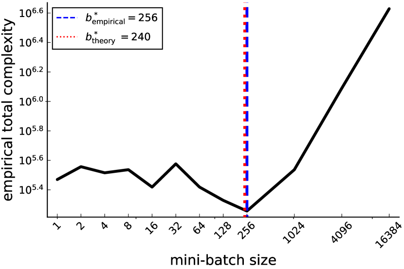
(a) ijcnn

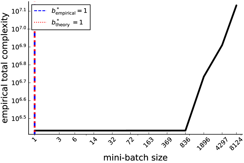
(b) mushrooms

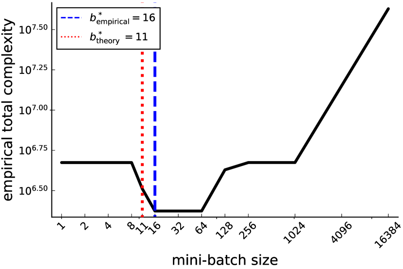
(c) phishing

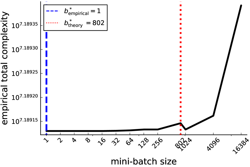
(d) YearPredictionMSD

Figure 1: Comparing the theoretical optimal batchsize (31) with the best over a grid.

In Figure 1 we plot the total complexity (number of iterations times the minibatch size) to reach this tolerance for each minibatch size on the grid. We can see in Figure 1 that for ijcnn and phishing the optimal minibatch size $b^{*}_{\text{theory}}=b^{*}_{saga}$ (31) is remarkably close to the best minibatch size over the grid $b^{*}_{\text{empirical}}$. Even when $b^{*}_{\text{theory}}$ is not close to $b^{*}_{\text{empirical}}$, such as on the YearPredictionMSD problem, the resulting total complexity is still very close to the total complexity of $b^{*}_{\text{empirical}}$.

Outline of the appendix.

The appendix is organized as follows:

• Section A: we present the arbitrary sampling framework for Stochastic Gradient methods introduced in [13], which will be used for the analysis of SGD and L-SVRG.

• Section B: we present specializations of Theorem 3.3 to the algorithms we discuss: SGD, DIANA, L-SVRG, SAGA and SEGA.

• Section C: we present the proof of our main Theorem 3.3.

• Section D: we present the proof of Corollary 4.2.

• Section E, we present the proof of Proposition 5.1, and the detailed analysis of the optimal minibatch results for $b$-SAGA and $b$-L-SVRG, in addition to an analysis for the optimal miniblock size for $b$-SEGA.

• Section F: we present some technical lemmas which we use in our analysis.

Appendix A Arbitrary Sampling

In this section, we recall the arbitrary sampling framework [12] which allows us to analyze our algorithms for minibatching, importance sampling and virtually all possible forms of sampling.

A.1 Stochastic reformulation

To see importance sampling and minibatch variants of stochastic gradient methods all through the same lens, we introduce a sampling vector which we will use to re-write (1).

Definition A.1.

We say that a random element-wise positive vector $v\in\mathbb{R}^{n}_{+}$ drawn from some distribution $\mathcal{D}$ is a sampling vector if its expectation is the vector of all ones:

$$\mathbb{E}_{\mathcal{D}}\left[v_{i}\right]=1,\text{ for all }i\in[n].$$ (34)

For a given distribution $\mathcal{D}$ we introduce a stochastic reformulation of (1) as follows

$$\min_{x\in\mathbb{R}^{d}}\ \left\{\mathbb{E}_{\mathcal{D}}\left[f_{v}(x)\overset{\text{def}}{=}\frac{1}{n}\sum_{i=1}^{n}v_{i}f_{i}(x)\right]+R(x)\right\}.$$ (35)

By definition of the sampling vector, $f_{v}(x)$ and $\nabla f_{v}(x)$ are unbiased estimators of $f(x)$ and $\nabla f(x)$, respectively, and hence problem (35) is indeed equivalent (i.e. a reformulation) of the original problem (1). In the case of the gradient, for instance, we get

$$\mathbb{E}_{\mathcal{D}}\left[\nabla f_{v}(x)\right]\overset{\eqref{eq:stochastic-reformulation}}{=}\frac{1}{n}\sum_{i=1}^{n}\mathbb{E}_{\mathcal{D}}\left[v_{i}\right]\nabla f_{i}(x)\overset{\eqref{eq:sampling-vector-def}}{=}\nabla f(x).$$ (36)

Reformulation (35) can be solved using proximal stochastic gradient descent via

$$x_{k+1}=\mathrm{prox}_{\gamma_{k}R}\left(x_{k}-\gamma\nabla f_{v_{k}}(x_{k})\right),$$ (37)

where $v_{k}\sim\mathcal{D}$ is sampled i.i.d. at each iteration and $\gamma>0$ is a stepsize. By substituting specific choices of $\mathcal{D}$, we obtain specific variants of SGD for solving (1). We further show that (37) is a special case of (2) with a sequence of vectors $g_{k}=\nabla f_{v_{k}}(x_{k})$ and use the unified analysis in Theorem 3.3 to obtain convergence rates for (37).

A.2 Expected Smoothness and Gradient Noise

In order to analyze (37) we will make use of the following result, which characterizes the smoothness of the subsampled functions $f_{v}$.

Lemma A.2.

(Expected Smoothness) If for all $i\in[n],f_{i}$ is convex and $L_{i}-$smooth, then there exists a constant $\mathcal{L}\geq 0$ such that

$$\mathbb{E}_{\mathcal{D}}\left[\left\lVert\nabla f_{v}(x)-\nabla f_{v}(x_{\ast})\right\rVert^{2}\right]\leq 2\mathcal{L}\,D_{f}(x,x_{\ast}),$$ (38)

for all $x\in\mathbb{R}^{d}$ and where $x_{\ast}$ is any minimizer of (1).

The proof of this results follows closely that of Lemma 1 in [9].

Proof.

Since for all $i\in[n]$, $f_{i}$ is $L_{i}$-smooth and convex, we have that each realization $f_{v}$ (defined in (35)) is $L_{v}$-smooth and convex. Thus, from Lemma F.1, we have that for all $x\in\mathbb{R}^{d}$,

$${\left\lVert\nabla f_{v}(x)-f_{v}(x_{*})\right\rVert}^{2} \leq 2L_{v}\left(f_{v}(x)-f_{v}(x_{*})-\left\langle\nabla f_{v}(x_{*}),x-x_{*}\right\rangle\right)$$

$$= \frac{2}{n}\sum_{i=1}^{n}L_{v}v_{i}\left(f_{i}(x)-f_{i}(x_{*})-\left\langle\nabla f_{i}(x_{*}),x-x_{*}\right\rangle\right).$$

Taking expectation over the samplings,

$$\mathbb{E}_{\mathcal{D}}\left[{\left\lVert\nabla f_{v}(x)-f_{v}(x_{*})\right\rVert}^{2}\right] \leq \frac{2}{n}\sum_{i=1}^{n}\mathbb{E}_{\mathcal{D}}\left[v_{i}L_{v}\right]\left(f_{i}(x)-f_{i}(x_{*})-\left\langle\nabla f_{i}(x_{*}),x-x_{*}\right\rangle\right)$$

$$\leq 2\max_{j=1,\dots,n}\mathbb{E}_{\mathcal{D}}\left[L_{v}v_{j}\right]\left(f(x)-f(x_{*})-\left\langle\nabla f(x_{*}),x-x_{*}\right\rangle\right)$$

$$= 2\max_{j=1,\dots,n}\mathbb{E}_{\mathcal{D}}\left[L_{v}v_{j}\right]D_{f}(x,x_{*}).$$

∎

Next, we define the gradient noise.

Definition A.3.

(Gradient Noise). The gradient noise $\sigma^{2}=\sigma^{2}(f,\mathcal{D})$ is defined by

$$\sigma^{2}\overset{\text{def}}{=}\mathbb{E}_{\mathcal{D}}\left[\left\lVert\nabla f_{v}(x_{\ast})-\nabla f(x_{\ast})\right\rVert^{2}\right].$$ (39)

A.3 Minibatching elements without replacement

Since analyzing minibatching for variance reduced methods is one of the main focuses of our work, we present minibatching without replacement as an example of the use of arbitrary sampling.

First, we define samplings.

Definition A.4 (Sampling).

A sampling $S\subseteq[n]$ is any random set-valued map which is uniquely defined by the probabilities $\sum_{B\subseteq[n]}p_{B}=1$ where $p_{B}\;\overset{\text{def}}{=}\;\mathbb{P}(S=B),\quad\forall B\subseteq[n].$ A sampling $S$ is called proper if for every $i\in[n]$, we have that $p_{i}\overset{\text{def}}{=}\mathbb{P}(i\in S)=\underset{C:i\in C}{\sum}p_{C}>0$.

We can build a sampling vector using a sampling as follows.

Lemma A.5 (Sampling vector, Lemma 3.3 in [12]).

Let $S$ be a proper sampling. Let $p_{i}\overset{\text{def}}{=}\mathbb{P}(i\in S)$ and $\mathbf{P}\overset{\text{def}}{=}\mathrm{diag}\left(p_{1},\dots,p_{n}\right)$. Let $v=v(S)$ be a random vector defined by

$$v(S)\;=\;\mathbf{P}^{-1}\sum_{i\in S}e_{i}\;\overset{\text{def}}{=}\;\mathbf{P}^{-1}e_{S}.$$ (40)

It follows that $v$ is a sampling vector.

Proof. The $i$-th coordinate of $v(S)$ is $v_{i}(S)=\mathbbm{1}(i\in S)/p_{i}$ and thus

$$\mathbb{E}\left[v_{i}(S)\right]\;=\;\frac{\mathbb{E}\left[\mathbbm{1}(i\in S)\right]}{p_{i}}\;=\;\frac{\mathbb{P}(i\in S)}{p_{i}}\;=\;1.\qquad\qquad\qed$$

Next, we define $b$-nice sampling, also known as minibatching without replacement.

Definition A.6 ($b$-nice sampling).

$S$ is a $b$-nice sampling if it is a sampling such that

$$\mathbb{P}(S=B)=\frac{1}{\binom{n}{b}},\quad\forall B\subseteq[n],\;\text{ with }\;|B|=b.$$

To construct such a sampling vector based on the $b$–nice sampling, note that $p_{i}=\tfrac{b}{n}$ for all $i\in[n]$ and thus we have that $v(S)=\tfrac{n}{b}\sum_{i\in S}e_{i}$ according to Lemma A.5. The resulting subsampled function is then $f_{v}(x)=\tfrac{1}{|S|}\sum_{i\in S}f_{i}(x)$, which is simply the minibatch average over $S$.

A remarkable result for $b$-nice sampling is that when all the functions $f_{i},i\in[n]$ are $L_{i}-$smooth and convex, then the expected smoothness constant (38) nicely interpolates between $L$, the smoothness constant of $f$, and $L_{\max}=\underset{i\in[n]}{\max}\,L_{i}$.

Lemma A.7 ($\mathcal{L}$ for $b-$nice sampling, Proposition 3.8 in [12]).

Let $v$ be a sampling vector based on the $b-$nice sampling defined in A.6. If for all $i\in[n],f_{i}$ is convex and $L_{i}-$smooth, then (38) holds with

$$\mathcal{L}(b)=\frac{1}{b}\frac{n-b}{n-1}L_{\max}+\frac{n}{b}\frac{b-1}{n-1}L,$$

where $L$ is the smoothness constant of $f$ and $L_{\max}=\underset{i\in[n]}{\max}\,L_{i}$.

Appendix B Notable Corollaries of Theorem 3.3

In this section, we present corollaries of Theorem 3.3 for five algorithms:

• SGD with arbitrary sampling (Algorithm 3).

• DIANA (Algorithm 4).

• L-SVRG with arbitrary sampling (Algorithm 5), and minibatch L-SVRG as a special case (Algorithm 2).

• Minibatch SAGA (Algorithm 1).

• Miniblock SEGA (Algorithm 6).

This means that for each method, we will present the constants which satisfy Assumption 3.2 and specialize Theorem 3.3 using these constants.

B.1 SGD with arbitrary sampling

Parameters step sizes $(\gamma_{k})_{k}$, a sampling vector $v\sim\mathcal{D}$

Initialization $x_{0}\in\mathbb{R}^{d}$

for $k=1,2,\dots$ do

     Sample $v_{k}\sim\mathcal{D}$

     $g_{k}=\nabla f_{v_{k}}(x_{k})$

     $x_{k+1}=\mathrm{prox}_{\gamma_{k}R}\left(x_{k}-\gamma_{k}g_{k}\right)$

end for

Algorithm 3 SGD-AS

Lemma B.1.

The iterates of Algorithm 3 satisfy Assumption 3.2 with

$$\sigma_{k}^{2}=0$$

and constants:

$$A=2\mathcal{L},\;B=0,\;\rho=1,\;C=0,\;D_{1}=2\sigma^{2},\;D_{2}=0,$$ (41)

where $\mathcal{L}$ is defined in (38) and $\sigma^{2}$ in (39).

Proof.

See Lemma A.2 in [11]. ∎

Using the constants given in the above lemma, we have the following immediate corollary of Theorem 3.3.

Corollary B.2.

Assume that $f$ has a finite-sum structure (4) and that Assumption 3.1 holds. Let $(\gamma_{k})_{k\geq 0}$ be a decreasing, strictly positive sequence of step sizes chosen such that

$$0<\gamma_{0}<\min\left\{\frac{1}{4\mathcal{L}},\frac{1}{L}\right\}.$$

Then, from Theorem 3.3 and Lemma B.1, we have that the iterates given by Algorithm 3 verify

$$\mathbb{E}\left[F(\bar{x}_{t})-F(x_{\ast})\right]\leq\frac{{\left\lVert x_{0}-x_{*}\right\rVert}^{2}+2\gamma_{0}\left(F(x_{0})-F(x_{*})\right)+4\sigma^{2}\sum_{k=0}^{t-1}\gamma_{k}^{2}}{2\sum_{i=0}^{t-1}\left(1-4\gamma_{i}\mathcal{L}\right)\gamma_{i}},$$ (42)

where $\bar{x}_{t}\overset{\text{def}}{=}\sum\limits_{k=0}^{t-1}\frac{\left(1-4\gamma_{k}\mathcal{L}\right)\gamma_{k}}{\sum_{i=0}^{t-1}\left(1-4\gamma_{i}\mathcal{L}\right)\gamma_{i}}x_{k}$.

B.2 DIANA

A complete description of the DIANA algorithm can be found in [26].

To analyze the DIANA algorithm (Algorithm 4), we introduce quantization operators.

Definition B.3 ($w$-quantization operator, Definition 4 in [26]).

Let $w>0$. A random operator $Q:\mathbb{R}^{d}\rightarrow\mathbb{R}$ with the properties:

$$\mathbb{E}\left[Q(x)\right]=x,\quad\mathbb{E}\left[{\left\lVert Q(x)\right\rVert}^{2}\right]\leq(1+w){\left\lVert x\right\rVert}^{2},$$ (43)

for all $x\in\mathbb{R}^{d}$ is called a $w$-quantization operator.

Several examples of quantization operators can be found in [26].

Parameters $w$-quantization operator $Q$, Learning rates $\alpha>0$ and $\gamma>0$, initial vectors $x^{0},h_{1}^{0},\dots,h_{n}^{0}\in\mathbb{R}^{d}$ and $h^{0}=\frac{1}{n}\sum\limits_{i=1}^{n}h_{i}^{0}$

Initialization $x^{0},h_{1}^{0},\dots,h_{n}^{0}\in\mathbb{R}^{d}$

Set $h^{0}=\frac{1}{n}\sum\limits_{i=1}^{n}h_{i}^{0}$

for $k=1,2,\dots$ do

     Broadcast $x_{k}$ to all workers.

     for $k=1,2,\dots$ do

         Sample $g_{i}^{k}$ such that $\mathbb{E}_{k}\left[g_{i}^{k}\right]=\nabla f_{i}(x_{k})$

         $\Delta_{i}^{k}=g_{i}^{k}-h_{i}^{k}$

         Sample $\hat{\Delta}_{i}^{k}\sim Q(\Delta_{i}^{k})$

         $h_{i}^{k+1}=h_{i}^{k}+\alpha\Delta_{i}^{k}$

         $\hat{g}_{i}^{k}=h_{i}^{k}+\hat{\Delta}_{i}^{k}$

     end for

     $\hat{\Delta}^{k}=\frac{1}{n}\sum\limits_{i=1}^{n}\Delta_{i}^{k}$

     $g_{k}=\frac{1}{n}\sum\limits_{i=1}^{n}\hat{g}_{i}^{k}=h^{k}+\hat{\Delta}^{k}$

     $x_{k+1}=\mathrm{prox}_{\gamma_{k}R}\left(x_{k}-\gamma_{k}g_{k}\right)$

     $h^{k+1}=\frac{1}{n}\sum\limits_{i=1}^{n}h_{i}^{k+1}=h^{k}+\alpha\hat{\Delta}^{k}$

end for

Algorithm 4 DIANA

For convenience, we repeat the statement of Lemma 4.5 below.

Lemma B.4.

Assume that $f$ has a finite sum structure and that Assumption 3.1 holds. The iterates of DIANA (Algorithm 4) satisfy Assumption 3.2 with constants:

$$A=\left(1+\frac{2w}{n}\right)L_{\max},\;B=\frac{2w}{n},\;\rho=\alpha,\;C=L_{\max}\alpha,\;D_{1}=\frac{(1+w)\sigma^{2}}{n},\;D_{2}=\alpha\sigma^{2},$$ (44)

where $w>0$ and $\alpha\leq\frac{1}{1+w}$ are parameters of Algorithm 4 and $\sigma^{2}$ is such that

$$\forall k\in\mathbb{N},\quad\frac{1}{n}\sum_{i=1}^{n}\mathbb{E}\left[{\left\lVert g_{i}^{k}-\nabla f(x_{k})\right\rVert}^{2}\right]\leq\sigma^{2}.$$

Proof.

See Lemma A.12 in [11]. ∎

Now using the constants given in the above lemma in Theorem 3.3 gives the following corollary.

Corollary B.5.

Assume that $f$ has a finite sum structure (4) and that Assumption 3.1 holds. Let $(\gamma_{k})_{k\geq 0}$ be a decreasing, strictly positive sequence of step sizes chosen such that

$$0<\gamma_{0}<\frac{1}{2(1+\frac{4w}{n})L_{\max}}.$$

Then, from Theorem 3.3 and Lemma B.4, we have that the iterates given by Algorithm 4 verify

$$\mathbb{E}\left[F(\bar{x}_{t})-F(x_{\ast})\right]\leq\frac{{\left\lVert x_{0}-x_{*}\right\rVert}^{2}+2\gamma_{0}\left(F(x_{0})-F(x_{*})+\frac{2w\gamma_{0}}{\alpha n}\sigma_{0}^{2}\right)+\frac{2\left(1+5w\right)\sigma^{2}}{n}\sum_{k=0}^{t-1}\gamma_{k}^{2}}{2\sum_{i=0}^{t-1}\left(1-\gamma_{i}\eta\right)\gamma_{i}},$$ (45)

where $\eta\overset{\text{def}}{=}2(1+\frac{4w}{n})L_{\max}$, $\bar{x}_{t}\overset{\text{def}}{=}\sum\limits_{k=0}^{t-1}\frac{\left(1-\gamma_{k}\eta\right)\gamma_{k}}{\sum_{i=0}^{t-1}\left(1-\gamma_{i}\eta\right)\gamma_{i}}x_{k}$ and ${\delta_{0}\overset{\text{def}}{=}F(x_{0})-F(x_{\ast})}$.

B.3 L-SVRG with arbitrary sampling

Parameters step size $\gamma$, sampling vector $v\sim\mathcal{D}$

Initialization $w_{0}=x_{0}\in\mathbb{R}^{d}$

for $k=1,2,\dots$ do

     Sample $v_{k}\sim\mathcal{D}$

     $g_{k}=\nabla f_{v_{k}}(x_{k})-\nabla f_{v_{k}}(w_{k})+\nabla f(w_{k})$

     $x_{k+1}=\mathrm{prox}_{\gamma R}\left(x_{k}-\gamma g_{k}\right)$

     $w_{k+1}=\left\{\begin{array}[]{ll}x_{k}&\mbox{with probability }p\\ w_{k}&\mbox{with probability }1-p\end{array}\right.$

end for

Algorithm 5 L-SVRG-AS

Lemma B.6.

If Assumption 3.1 holds then the iterates of Algorithm 5 satisfy

$$\mathbb{E}_{k}\left[{\left\lVert g_{k}-\nabla f(x_{*})\right\rVert}^{2}\right] \leq 4\mathcal{L}D_{f}(x_{k},x_{*})+2\sigma_{k}^{2}$$ (46)

$$\mathbb{E}_{k}\left[\sigma_{k+1}^{2}\right] \leq (1-p)\sigma_{k}^{2}+2p\mathcal{L}D_{f}(x_{k},x_{*}),$$ (47)

where

$$\sigma_{k}^{2}=\mathbb{E}_{\mathcal{D}}\left[{\left\lVert\nabla f_{v_{k}}(w_{k})-\nabla f_{v_{k}}(x_{*})-\left(\nabla f(w_{k})-\nabla f(x_{*})\right)\right\rVert}^{2}\right]$$ (48)

and $\mathcal{L}$ is defined in (38).

Proof.

By Lemma A.2 we have that (38) holds with $\mathcal{L}>0.$ Furthermore

$$\mathbb{E}_{k}\left[{\left\lVert g_{k}\right\rVert}^{2}\right] = \mathbb{E}_{k}\left[{\left\lVert\nabla f_{v_{k}}(x_{k})-\nabla f_{v_{k}}(w_{k})+\nabla f(w_{k})-\nabla f(x_{*})\right\rVert}^{2}\right]$$

$$\leq 2\mathbb{E}_{k}\left[{\left\lVert\nabla f_{v_{k}}(x_{k})-\nabla f_{v_{k}}(x_{*})\right\rVert}^{2}\right]$$

$$+2\mathbb{E}_{k}\left[{\left\lVert\nabla f_{v_{k}}(w_{k})-\nabla f_{v_{k}}(x_{*})-\left(\nabla f(w_{k})-\nabla f(x_{*})\right)\right\rVert}^{2}\right],$$

where we used in the inequality that for all $a,b\in\mathbb{R}^{d},{\left\lVert a+b\right\rVert}^{2}\leq 2{\left\lVert a\right\rVert}^{2}+2{\left\lVert b\right\rVert}^{2}$. Thus,

$$\mathbb{E}_{k}\left[{\left\lVert g_{k}\right\rVert}^{2}\right]\overset{\eqref{eq:expected-smoothness}}{\leq}4\mathcal{L}D_{f}\left(x_{k},x_{*}\right)+2\sigma_{k}^{2}.$$

Moreover,

$$\mathbb{E}_{k}\left[\sigma_{k+1}\right] = (1-p)\sigma_{k}^{2}+p\mathbb{E}_{k}\left[{\left\lVert\nabla f_{v_{k}}(x_{k})-\nabla f_{v_{k}}(x_{*})-\left(\nabla f(x_{k})-\nabla f(x_{*})\right)\right\rVert}^{2}\right]$$

$$\overset{\eqref{eq:expected-smoothness}}{\leq} (1-p)\sigma_{k}^{2}+2p\mathcal{L}D_{f}\left(x_{k},x_{*}\right),$$

where we also used in the last inequality that $\mathbb{E}\left[\left\lVert X-\mathbb{E}\left[X\right]\right\rVert^{2}\right]=\mathbb{E}\left[\left\lVert X\right\rVert^{2}\right]-\left\lVert\mathbb{E}\left[X\right]\right\rVert^{2}\leq\mathbb{E}\left[\left\lVert X\right\rVert^{2}\right]$. ∎

We have the following immediate consequence of the previous lemma.

Lemma B.7.

If Assumption 3.1 holds then the iterates of Algorithm 5 satisfy Assumption 3.2 with

$$\sigma_{k}^{2}=\mathbb{E}_{\mathcal{D}}\left[{\left\lVert\nabla f_{v}(x_{k})-\nabla f_{v}(w_{k})+\nabla f(w_{k})\right\rVert}^{2}\right]$$

and constants

$$A=2\mathcal{L},\;B=2,\;\rho=p,\;C=p\mathcal{L},\;D_{1}=D_{2}=0,$$ (49)

where $\mathcal{L}$ is defined in (38).

Using the constant derived in Lemma B.7 in Theorem 3.3 gives the following corollary.

Corollary B.8.

Assume that $f$ has a finite sum structure (4) and that Assumption 3.1 holds. Let $\gamma_{k}=\gamma$ for all $k\in\mathbb{N}$, where

$$0<\gamma<\min\left\{\frac{1}{8\mathcal{L}},\frac{1}{L}\right\}.$$

Then, from Theorem 3.3 and Lemma B.7, we have that the iterates given by Algorithm 5 verify

$$\mathbb{E}\left[F(\bar{x}_{t})-F(x_{\ast})\right]\leq\frac{{\left\lVert x_{0}-x_{*}\right\rVert}^{2}+2\gamma\left(F(x_{0})-F(x_{*})+\frac{2\gamma}{p}\sigma_{0}^{2}\right)}{2\gamma\left(1-8\gamma\mathcal{L}\right)t},$$ (50)

where $\bar{x}_{t}\overset{\text{def}}{=}\frac{1}{t}\sum\limits_{k=0}^{t-1}x_{k}$ and where $\mathcal{L}$ is defined in (38).

B.3.1 $b$-L-SVRG

As we demonstrated in Section A.3, we can specialize the results derived for arbitrary sampling to minibatching without replacement by using a $b-$nice sampling defined in Definition A.6 and the corresponding sampling vector (40).

Indeed, using Algorithm 5 with $b$-nice sampling is equivalent to using Algorithm 2. Thus, we have the following lemma.

Corollary B.9.

From Lemma B.7, we have that the iterates of Algorithm 2 satisfy Assumption 3.2 with constants:

$$A=2\mathcal{L}(b),\;B=2,\;\rho=p,\;C=p\mathcal{L}(b),\;D_{1}=D_{2}=0,$$ (51)

where $\mathcal{L}(b)$ is defined in (24).

A convergence result for Algorithm 2 can be easily concluded from Corollary B.8, with $\mathcal{L}(b)$ in place of $\mathcal{L}$.

B.4 $b$-SAGA

Lemma 5.3 in the main text is a consequence of the following lemma.

Lemma B.10.

Consider the iterates of Algorithm 1. We have:

$$\mathbb{E}_{k}\left[{\left\lVert g_{k}\right\rVert}^{2}\right] \leq 4\mathcal{L}(b)\left(f(x_{k})-f(x_{*})\right)+2\sigma_{k}^{2}$$ (52)

$$\mathbb{E}_{k}\left[\sigma_{k+1}^{2}\right] \leq (1-\frac{b}{n})\sigma_{k}^{2}+2\frac{b\zeta(b)}{n}\left(f(x_{k})-f(x_{*})\right),$$ (53)

where:

$$\sigma_{k}^{2}=\frac{1}{nb}\frac{n-b}{n-1}{\left\lVert J_{k}-\nabla H(x_{*})\right\rVert}^{2}_{\mathrm{Tr}}\quad\mbox{and}\quad\zeta(b)\overset{\text{def}}{=}\frac{1}{b}\frac{n-b}{n-1}L_{\max},$$ (54)

with ${\left\lVert Z\right\rVert}^{2}_{\mathrm{Tr}}=\mathrm{Tr}(Z^{\top}Z)$ for any $Z\in\mathbb{R}^{d\times n}$.

Proof.

The inequality (52) corresponds to Lemma 3.10 and (53) to Lemma 3.9 in [13]. ∎

The previous Lemma gives us the constants for Assumption 3.2 for Algorithm 1.

Lemma B.11.

The iterates of Algorithm 1 satisfy Assumption 3.2 with

$$\sigma_{k}^{2}=\frac{1}{nb}\frac{n-b}{n-1}{\left\lVert J_{k}-\nabla H(x_{*})\right\rVert}^{2}_{\mathrm{Tr}}$$ (55)

and constants

$$A=2\mathcal{L}(b),\;B=2,\;\rho=\frac{b}{n},\;C=\frac{b\zeta(b)}{n},\;D_{1}=D_{2}=0.$$ (56)

Using the constant derived in Lemma B.11 in Theorem 3.3 gives the following corollary.

Corollary B.12.

Assume that $f$ has a finite sum structure (4) and that Assumption 3.1 holds. Choose for all $k\in\mathbb{N}$ $\gamma_{k}=\gamma$, where

$$0<\gamma<\frac{1}{2(2\mathcal{L}(b)+\zeta(b))}.$$

Then, from Theorem 3.3 and Lemma B.11, we have that the iterates given by Algorithm 1 verify

$$\mathbb{E}\left[F(\bar{x}_{t})-F(x_{\ast})\right]\leq\frac{{\left\lVert x_{0}-x_{*}\right\rVert}^{2}+2\gamma\left(F(x_{0})-F(x_{*})+\frac{2n\gamma}{b}\sigma_{0}^{2}\right)}{2\gamma\left(1-2\gamma\left(2\mathcal{L}(b)+2\zeta(b)\right)\right)t},$$ (57)

where $\bar{x}_{t}\overset{\text{def}}{=}\frac{1}{t}\sum\limits_{k=0}^{t-1}x_{k}$.

B.5 $b$-SEGA

Lemma B.13.

Consider the iterates of Algorithm 6. We have:

$$\mathbb{E}_{k}\left[{\left\lVert g_{k}\right\rVert}^{2}\right] \leq \frac{4dL}{b}D_{f}\left(x_{k},x_{*}\right)+2\left(\frac{d}{b}-1\right)\sigma_{k}^{2}$$ (58)

$$\mathbb{E}_{k}\left[\sigma_{k+1}^{2}\right] \leq (1-\frac{b}{d})\sigma_{k}^{2}+\frac{2bL}{d}D_{f}\left(x_{k},x_{*}\right),$$ (59)

where:

$$\sigma_{k}^{2}={\left\lVert h_{k}-\nabla f(x_{*})\right\rVert}^{2}.$$ (60)

Proof.

Let $S$ be a random miniblock s.t. $\mathbb{P}(S=B)=\frac{1}{\binom{n}{b}}$ for any $B\subseteq[n]$ s.t. $|B|=b$. Then, for any vector $a=[a_{1},\dots,a_{n}]\in\mathbb{R}^{d}$, we have:

$$\mathbb{E}\left[{\left\lVert I_{S}a\right\rVert}^{2}\right]=\frac{b}{d}{\left\lVert a\right\rVert}^{2}\quad\mbox{and}\quad\mathbb{E}\left[{\left\lVert(I-\frac{d}{b}I_{S})a\right\rVert}^{2}\right]=\left(\frac{d}{b}-1\right){\left\lVert a\right\rVert}^{2}.$$ (61)

Indeed,

$$\mathbb{E}\left[{\left\lVert I_{S}a\right\rVert}^{2}\right] = \mathbb{E}\left[\sum_{i\in S}a_{i}^{2}\right]=\sum_{B\subseteq[d],|B|=b}\mathbb{P}(S=B)\sum_{i\in B}a_{i}^{2}=\frac{1}{\binom{d}{b}}\sum_{B\subseteq[d],|B|=b}\sum_{i=1}^{d}a_{i}^{2}\mathbbm{1}_{B}(i)$$

$$= \frac{1}{\binom{d}{b}}\sum_{i=1}^{d}a_{i}^{2}\sum_{B\subseteq[d],|B|=b}\mathbbm{1}_{B}(i)=\frac{\binom{d-1}{b-1}}{\binom{d}{b}}\sum_{i=1}^{d}a_{i}^{2}=\frac{b}{d}{\left\lVert a\right\rVert}^{2},$$

where we used that $|B\in[d]:|B|=b\land i\in B|=\binom{d-1}{b-1}$. And

$${\left\lVert(I-\frac{d}{b}I_{S})a\right\rVert}^{2} = \sum_{i\in S}\left(1-\frac{d}{b}\right)^{2}a_{i}^{2}+\sum_{i\notin S}a_{i}^{2}=\frac{d^{2}-2bd}{b^{2}}\sum_{i\in S}a_{i}^{2}+{\left\lVert a\right\rVert}^{2}$$

$$= \frac{d^{2}-2bd}{b^{2}}{\left\lVert I_{S}a\right\rVert}^{2}+{\left\lVert a\right\rVert}^{2}.$$

Thus,

$$\mathbb{E}\left[\left\lVert(I-\frac{d}{b}I_{S})a\right\rVert^{2}\right]=\left(\frac{d^{2}-2bd}{b^{2}}\frac{b}{d}+1\right){\left\lVert a\right\rVert}^{2}=\left(\frac{d}{b}-1\right){\left\lVert a\right\rVert}^{2}.$$

We have

$$\mathbb{E}_{k}\left[{\left\lVert g_{k}-\nabla f(x_{*})\right\rVert}^{2}\right] = \mathbb{E}_{k}\left[{\left\lVert\frac{d}{b}I_{B_{k}}(\nabla f(x_{k})-\nabla f(x_{*}))+\left(I-\frac{d}{b}I_{B_{k}}\right)(h_{k}-\nabla f(x_{*}))\right\rVert}^{2}\right]$$

$$\leq \frac{2d^{2}}{b^{2}}\mathbb{E}_{k}\left[{\left\lVert I_{B_{k}}(\nabla f(x_{k})-\nabla f(x_{*}))\right\rVert}^{2}\right]+2\mathbb{E}_{k}\left[{\left\lVert\left(I-\frac{d}{b}I_{B_{k}}\right)(h_{k}-\nabla f(x_{*}))\right\rVert}^{2}\right]$$

$$\overset{\eqref{eq:sqn-sampled-miniblock}}{=} \frac{2d}{b}{\left\lVert\nabla f(x_{k})-\nabla f(x_{*})\right\rVert}^{2}+2\left(\frac{d}{b}-1\right){\left\lVert h_{k}-\nabla f(x_{*})\right\rVert}^{2}.$$

where we used in the first inequality that for all $a,b\in\mathbb{R}^{d},{\left\lVert a+b\right\rVert}^{2}\leq 2{\left\lVert a\right\rVert}^{2}+2{\left\lVert b\right\rVert}^{2}$. Thus, using the fact that $f$ is $L$-smooth, we have

$$\mathbb{E}_{k}\left[{\left\lVert g_{k}\right\rVert}^{2}\right]\leq\frac{4dL}{b}D_{f}\left(x_{k},x_{*}\right)+2\left(\frac{d}{b}-1\right)\sigma_{k}^{2}.$$

Moreover,

$$\mathbb{E}_{k}\left[\sigma_{k+1}^{2}\right] = \mathbb{E}_{k}\left[{\left\lVert h_{k+1}-\nabla f(x_{*})\right\rVert}^{2}\right]=\mathbb{E}_{k}\left[{\left\lVert I_{B_{k}^{c}}(h_{k}-\nabla f(x_{*}))+I_{B_{k}}(\nabla f(x_{k})-\nabla f(x_{*}))\right\rVert}^{2}\right]$$

$$\overset{\eqref{eq:sqn-sampled-miniblock}}{=} \left(1-\frac{b}{d}\right){\left\lVert h_{k}-\nabla f(x_{*})\right\rVert}^{2}+\frac{b}{d}{\left\lVert\nabla f(x_{k})-\nabla f(x_{*})\right\rVert}^{2}$$

$$+2\left\langle I_{B_{k}^{c}}(h_{k}-\nabla f(x_{*})),I_{B_{k}}(\nabla f(x_{k})-\nabla f(x_{*}))\right\rangle$$

$$= \left(1-\frac{b}{d}\right){\left\lVert h_{k}-\nabla f(x_{*})\right\rVert}^{2}+\frac{b}{d}{\left\lVert\nabla f(x_{k})-\nabla f(x_{*})\right\rVert}^{2}$$

$$+2\left\langle\underbrace{I_{B_{k}}I_{B_{k}^{c}}}_{=0}(h_{k}-\nabla f(x_{*})),\nabla f(x_{k})-\nabla f(x_{*})\right\rangle$$

$$\leq \left(1-\frac{b}{d}\right){\left\lVert h_{k}-\nabla f(x_{*})\right\rVert}^{2}+\frac{2bL}{d}D_{f}\left(x_{k},x_{*}\right),$$

where we used in the last inequality the $L-$smoothness of $f$. ∎

Lemma B.14.

From Lemma B.13, we have that the iterates of Algorithm 6 satisfy Assumption 3.2 and Equation (22) with

$$\sigma_{k}^{2}={\left\lVert h_{k}-\nabla f(x_{*})\right\rVert}^{2}$$ (62)

and constants:

$$A=\frac{2dL}{b},\;B=2\left(\frac{d}{b}-1\right),\;\rho=\frac{b}{d},\;C=\frac{bL}{d},\;D_{1}=D_{2}=0,\;G=0.$$ (63)

Using the constant derived in Lemma B.14 in Theorem 3.3 gives the following corollary.

Corollary B.15.

Assume that $f$ satisfies Assumption 3.1. Choose for all $k\in\mathbb{N}$, $\gamma_{k}=\gamma$, where

$$0<\gamma<\frac{1}{4(\frac{2d}{b}-1)L}.$$

Then, from Theorem 3.3 and Lemma B.14, we have that the iterates given by Algorithm 6 verify

$$\mathbb{E}\left[F(\bar{x}_{t})-F(x_{\ast})\right]\leq\frac{{\left\lVert x_{0}-x_{*}\right\rVert}^{2}+2\gamma\left(F(x_{0})-F(x_{*})+\frac{2d}{b}\left(\frac{d}{b}-1\right)\gamma\sigma^{2}\right)}{2\gamma\left(1-4\gamma\left(\frac{2d}{b}-1\right)\right)t},$$ (64)

where $\bar{x}_{t}\overset{\text{def}}{=}\frac{1}{t}\sum\limits_{k=0}^{t-1}x_{k}$.

Appendix C Proofs for Section 3

C.1 Proof of Theorem 3.3

Before proving Theorem 3.3, we present several useful lemmas.

Lemma C.1 (Bounding the gradient variance).

Assuming that the $g_{k}$ are unbiased and that Assumption 3.2 holds, we have

$$\mathbb{E}\left[\left\lVert g_{k}-\nabla f(x_{k})\right\rVert^{2}\right]\leq 2AD_{f}(x_{k},x_{\ast})+B\sigma_{k}^{2}+D_{1}$$ (65)

Proof.

Starting from the left hand side of (65), we have

$$\mathbb{E}\left[\left\lVert g_{k}-\nabla f(x_{k})\right\rVert^{2}\right] =\mathbb{E}\left[\left\lVert g_{k}-\nabla f(x_{\ast})-\left(\nabla f(x_{k})-\nabla f(x_{\ast})\right)\right\rVert^{2}\right]$$

$$=\mathbb{E}\left[\left\lVert g_{k}-\nabla f(x_{\ast})-\mathbb{E}\left[g_{k}-\nabla f(x_{\ast})\right]\right\rVert^{2}\right]$$

$$\leq\mathbb{E}\left[\left\lVert g_{k}-\nabla f(x_{\ast})\right\rVert^{2}\right]\leq 2AD_{f}(x_{k},x_{\ast})+B\sigma_{k}^{2}+D_{1},$$

where we used that $\mathbb{E}\left[\left\lVert X-\mathbb{E}\left[X\right]\right\rVert^{2}\right]=\mathbb{E}\left[\left\lVert X\right\rVert^{2}\right]-\left\lVert\mathbb{E}\left[X\right]\right\rVert^{2}\leq\mathbb{E}\left[\left\lVert X\right\rVert^{2}\right]$ for any random variable $X$. ∎

Lemma C.2.

Suppose that Assumption 3.1 holds and let $\gamma\in\left(0,\frac{1}{L}\right]$, then for all $x,y\in\mathbb{R}^{d}$ and $p=\mathrm{prox}_{\gamma g}(y)$ we have,

$$-2\gamma\left(F(p)-F(x_{\ast})\right)\geq{\left\lVert p-z\right\rVert}^{2}+2\left\langle p-x_{\ast},x-\gamma\nabla f(x)-y\right\rangle-{\left\lVert x_{\ast}-x\right\rVert}^{2}.$$ (66)

Proof.

We leave the proof to Section F.3. ∎

Lemma C.3.

For any $x\in\mathbb{R}^{d}$ and minimizer $x_{\ast}$ of $F$ we have,

$$D_{f}(x,x_{\ast})\leq F(x)-F(x_{\ast}).$$ (67)

Proof.

Because $x_{\ast}$ is a minimizer of $F$ we have that $-\nabla f(x_{\ast})\in\partial R(x_{\ast})$. By the definition of subgradients we have

$$R(x_{\ast})+\left\langle-\nabla f(x_{\ast}),x-x_{\ast}\right\rangle\leq R(x).$$

Rearranging gives

$$-\left\langle\nabla f(x_{\ast}),x-x_{\ast}\right\rangle\leq R(x)-R(x_{\ast})$$

Adding $f(x)-f(x_{\ast})$ to both sides we have,

$$f(x)-f(x_{\ast})-\left\langle\nabla f(x_{\ast}),x-x_{\ast}\right\rangle\leq f(x)+R(x)-\left(f(x_{\ast})+R(x_{\ast})\right)=F(x)-F(x_{\ast}).$$

Now note that the on the left hand side we have the Bregman divergence $D_{f}(x,x_{\ast})$. ∎

Definition C.4.

Given a stepsize $\gamma>0$, the prox-grad mapping is defined as:

$$T_{\gamma}(x)\overset{\text{def}}{=}\mathrm{prox}_{\gamma R}\left(x-\gamma\nabla f(x)\right).$$ (68)

For the ease of exposition, we restate Theorem 3.3.

Theorem C.5.

Suppose that Assumptions 3.2 and 3.1 hold. Let $M\overset{\text{def}}{=}B/\rho$ and let $(\gamma_{k})_{k\geq 0}$ be a decreasing, strictly positive sequence of step sizes chosen such that

$$0<\gamma_{0}<\frac{1}{2(A+MC)}.$$

The iterates given by (2) converge according to

$$\mathbb{E}\left[F(\bar{x}_{t})-F(x_{\ast})\right]\leq\frac{V_{0}+2\gamma_{0}\delta_{0}+2\left(D_{1}+2MD_{2}\right)\sum_{k=0}^{t-1}\gamma_{k}^{2}}{2\sum_{i=0}^{t-1}\left(1-2\gamma_{i}\left(A+MC\right)\right)\gamma_{i}},$$ (69)

where $\bar{x}_{t}\overset{\text{def}}{=}\sum\limits_{k=0}^{t-1}\frac{\left(1-\gamma_{k}\eta\right)\gamma_{k}}{\sum_{i=0}^{t-1}\left(1-\gamma_{i}\eta\right)\gamma_{i}}x_{k}$ and $V_{0}\overset{\text{def}}{=}{\left\lVert x_{0}-x_{\ast}\right\rVert}^{2}+2\gamma_{0}^{2}M\sigma_{0}^{2}$ and ${\delta_{0}\overset{\text{def}}{=}F(x_{0})-F(x_{\ast})}$.

Proof.

Let $x_{\ast}$ be a minimizer of $F$. Using (66) from Lemma C.2 with $y=x_{k}-\gamma_{k}g_{k}$, $x=x_{k}$ and $\gamma=\gamma_{k}$ gives

$$-2\gamma_{k}\left(F(x_{k+1})-F(x_{\ast})\right) \geq\left\lVert x_{k+1}-x_{\ast}\right\rVert^{2}-\left\lVert x_{k}-x_{\ast}\right\rVert^{2}+2\gamma_{k}\left\langle x_{k+1}-x_{\ast},g_{k}-\nabla f(x_{k})\right\rangle.$$

Multiplying both sides by $-1$ results in

$$2\gamma_{k}\left(F(x_{k+1})-F(x_{\ast})\right) \leq{\left\lVert x_{k}-x_{\ast}\right\rVert}^{2}-{\left\lVert x_{k+1}-x_{\ast}\right\rVert}^{2}+2\gamma_{k}\left\langle x_{k+1}-x_{\ast},\nabla f(x_{k})-g_{k}\right\rangle.$$ (70)

Now focusing on the last term in the above and consider the straightforward decomposition

$$\left\langle x_{k+1}-x_{\ast},\nabla f(x_{k})-g_{k}\right\rangle =\left\langle x_{k+1}-T_{\gamma_{k}}(x_{k}),\nabla f(x_{k})-g_{k}\right\rangle+\left\langle T_{\gamma_{k}}(x_{k})-x_{\ast},\nabla f(x_{k})-g_{k}\right\rangle.$$ (71)

By Cauchy Schwartz we have that

$$\left\langle x_{k+1}-T_{\gamma_{k}}(x_{k}),\nabla f(x_{k})-g_{k}\right\rangle\leq\left\lVert x_{k+1}-T_{\gamma_{k}}(x_{k})\right\rVert\left\lVert g_{k}-\nabla f(x_{k})\right\rVert.$$ (72)

Now using the nonexpansivity of the proximal operator

$$\left\lVert x_{k+1}-T_{\gamma_{k}}(x_{k})\right\rVert =\left\lVert\mathrm{prox}_{\gamma_{k}R}\left(x_{k}-\gamma_{k}g_{k}\right)-\mathrm{prox}_{\gamma_{k}R}\left(x_{k}-\gamma_{k}\nabla f(x_{k})\right)\right\rVert$$

$$\leq\left\lVert\left(x_{k}-\gamma_{k}g_{k}\right)-\left(x_{k}-\gamma_{k}\nabla f(x_{k})\right)\right\rVert=\gamma_{k}\left\lVert g_{k}-\nabla f(x_{k})\right\rVert.$$

Using this in (72), we have

$$\left\langle x_{k+1}-T_{\gamma_{k}}(x_{k}),\nabla f(x_{k})-g_{k}\right\rangle\leq\gamma_{k}\left\lVert g_{k}-\nabla f(x_{k})\right\rVert^{2}.$$ (73)

Using (73) in (71) and taking expectation conditioned on $x_{k}$, and using $\mathbb{E}_{k}\left[\cdot\right]\overset{\text{def}}{=}\mathbb{E}\left[\cdot\;|\;x_{k}\right]$ for shorthand, we have

$$\mathbb{E}_{k}\left[\left\langle x_{k+1}-x_{\ast},g_{k}-\nabla f(x_{k})\right\rangle\right] \leq\gamma_{k}\cdot\mathbb{E}_{k}\left[\left\lVert g_{k}-\nabla f(x_{k})\right\rVert^{2}\right]+\left\langle T_{\gamma_{k}}(x_{k})-x_{\ast},\underbrace{\mathbb{E}_{k}\left[\nabla f(x_{k})-g_{k}\right]}_{=0}\right\rangle$$

$$=\gamma_{k}\cdot\mathbb{E}_{k}\left[\left\lVert g_{k}-\nabla f(x_{k})\right\rVert^{2}\right].$$ (74)

Let $r_{k}\overset{\text{def}}{=}x_{k}-x_{\ast}.$ Taking expectation conditioned on $x_{k}$ in (70) and using (C.1), we have

$$2\gamma_{k}\mathbb{E}_{k}\left[F(x_{k+1}-F(x_{\ast}))\right] \leq{\left\lVert r_{k}\right\rVert}^{2}-\mathbb{E}_{k}\left[\left\lVert r_{k+1}\right\rVert^{2}\right]+2\gamma_{k}^{2}\mathbb{E}_{k}\left[\left\lVert g_{k}-\nabla f(x_{k})\right\rVert^{2}\right].$$

Using (9) from Assumption 3.2 we have

$$2\gamma_{k}\mathbb{E}_{k}\left[F(x_{k+1})-F(x_{\ast})\right] \leq{\left\lVert r_{k}\right\rVert}^{2}-\mathbb{E}_{k}\left[\left\lVert r_{k+1}\right\rVert^{2}\right]+2\gamma_{k}^{2}\left(2AD_{f}(x_{k},x_{\ast})+B\sigma_{k}^{2}+D_{1}\right).$$

Let $V_{k}\overset{\text{def}}{=}{\left\lVert r_{k}\right\rVert}^{2}+2M\gamma_{k}^{2}\sigma_{k}^{2}$ where $M=\frac{B}{\rho}$, then

$$\begin{split}2\gamma_{k}\mathbb{E}_{k}\left[F(x_{k+1})-F(x_{\ast})\right]\leq V_{k}&-\mathbb{E}_{k}\left[V_{k+1}\right]+4\gamma_{k}^{2}AD_{f}(x_{k},x_{\ast})+2\gamma_{k}^{2}D_{1}\\ &+\gamma_{k}^{2}\left(2B-2M\right)\sigma_{k}^{2}+2M\gamma_{k+1}^{2}\mathbb{E}\left[\sigma_{k+1}^{2}\right].\end{split}$$ (75)

Since $\gamma_{k+1}\leq\gamma_{k}$ we have that

$$\begin{split}2\gamma_{k+1}\mathbb{E}_{k}\left[F(x_{k+1})-F(x_{\ast})\right]\leq V_{k}&-\mathbb{E}_{k}\left[V_{k+1}\right]+4\gamma_{k}^{2}AD_{f}(x_{k},x_{\ast})+2\gamma_{k}^{2}D_{1}\\ &+\gamma_{k}^{2}\left(2B-2M\right)\sigma_{k}^{2}+2M\gamma_{k}^{2}\mathbb{E}\left[\sigma_{k+1}^{2}\right].\end{split}$$ (76)

Using (10) from Assumption 3.2, we have

$$2\gamma_{k}^{2}\left(B-M\right)\sigma_{k}^{2}+2M\gamma_{k}^{2}\mathbb{E}_{k}\left[\sigma_{k+1}^{2}\right] \leq 2\gamma_{k}^{2}\left(B-M+M(1-\rho)\right)\sigma_{k}^{2}+4M\gamma_{k}^{2}CD_{f}(x_{k},x_{\ast})$$

$$\quad+2M\gamma_{k}^{2}D_{2}$$

$$=2\gamma_{k}^{2}\underbrace{\left(B-\rho M\right)}_{=0}\sigma_{k}^{2}+4M\gamma_{k}^{2}CD_{f}(x_{k},x_{\ast})+2M\gamma_{k}^{2}D_{2}$$

$$\leq 4M\gamma_{k}^{2}CD_{f}(x_{k},x_{\ast})+2M\gamma_{k}^{2}D_{2}.$$ (77)

Using (C.1) in (75) gives

$$2\gamma_{k+1}\mathbb{E}_{k}\left[F(x_{k+1})-F(x_{\ast})\right] \leq V_{k}-\mathbb{E}_{k}\left[V_{k+1}\right]+2\gamma_{k}^{2}\left(2A+2MC\right)D_{f}(x_{k},x_{\ast})+2\gamma_{k}^{2}\left(D_{1}+MD_{2}\right).$$ (78)

Let $\eta\overset{\text{def}}{=}2A+2MC$. Using (67) in (78) we have,

$$2\gamma_{k+1}\mathbb{E}_{k}\left[F(x_{k+1})-F(x_{\ast})\right] \leq V_{k}-\mathbb{E}_{k}\left[V_{k+1}\right]+2\gamma_{k}^{2}\eta\left(F(x_{k})-F(x_{\ast})\right)+2\gamma_{k}^{2}\left(D_{1}+MD_{2}\right).$$

Using the abbreviation $\delta_{k}=F(x_{k})-F(x_{\ast})$ gives

$$2\gamma_{k+1}\mathbb{E}_{k}\left[\delta_{k+1}\right] \leq V_{k}-\mathbb{E}_{k}\left[V_{k+1}\right]+2\gamma_{k}^{2}\eta\delta_{k}+2\gamma_{k}^{2}\left(D_{1}+MD_{2}\right).$$

Taking expectation,

$$2\gamma_{k+1}\mathbb{E}\left[\delta_{k+1}\right] \leq\mathbb{E}\left[V_{k}\right]-\mathbb{E}\left[V_{k+1}\right]+2\gamma_{k}^{2}\eta\mathbb{E}\left[\delta_{k}\right]+2\gamma_{k}^{2}\left(D_{1}+MD_{2}\right),$$

summing over $k=0,\ldots,t-1$ and using telescopic cancellation gives

$$2\sum_{k=1}^{t}\gamma_{k}\mathbb{E}\left[\delta_{k}\right] \leq V_{0}-\mathbb{E}\left[V_{t}\right]+2\eta\sum_{k=0}^{t-1}\gamma_{k}^{2}\mathbb{E}\left[\delta_{k}\right]+2\left(D_{1}+MD_{2}\right)\sum_{k=0}^{t-1}\gamma_{k}^{2}.$$

Adding $2\gamma_{0}\delta_{0}$ to both sides of the above inequality and rearranging,

$$2\sum_{k=0}^{t-1}\gamma_{k}(1-\eta\gamma_{k})\mathbb{E}\left[\delta_{k}\right] \leq V_{0}-\mathbb{E}\left[V_{t}\right]+2\gamma_{0}\delta_{0}+2\left(D_{1}+MD_{2}\right)\sum_{k=0}^{t-1}\gamma_{k}^{2}$$

where we also used that $V_{t}\geq 0$ and $\delta_{t}\geq 0.$

By the choice of $\gamma_{0}$ we have $1-\gamma_{0}\eta>0$, and since $(\gamma_{i})_{i}$ is a decreasing sequence, we have $1-\gamma_{i}\eta>0$ for all $i$. Hence dividing both sides by $2\sum\limits_{i=0}^{t-1}\left(1-\gamma_{i}\eta\right)\gamma_{i}$, we have

$$\sum_{k=0}^{t-1}w_{k}\mathbb{E}\left[\delta_{k}\right]\leq\frac{V_{0}+2\gamma_{0}\delta_{0}}{2\sum_{i=0}^{t-1}\left(1-\gamma_{i}\eta\right)\gamma_{i}}+\left(D_{1}+2MD_{2}\right)\frac{\sum_{k=0}^{t-1}\gamma_{k}^{2}}{\sum_{i=1}^{t}\left(1-\gamma_{i}\eta\right)\gamma_{i}},$$

where $w_{k}\overset{\text{def}}{=}\frac{\left(1-\gamma_{k}\eta\right)\gamma_{k}}{\sum_{i=0}^{t-1}\left(1-\gamma_{i}\eta\right)\gamma_{i}}$ for all $k\in\left\{0,\dots,t-1\right\}$. Note that $\sum_{k=0}^{t-1}w_{k}=1$ and $w_{k}\geq 0$ for all $k\in\left\{0,\dots,t-1\right\}$. Hence, since $F$ is convex, we can use Jensen’s inequality to conclude

$$\mathbb{E}\left[F(\bar{x}^{k})-F(x_{\ast})\right] =\mathbb{E}\left[F\left(\sum\limits_{k=0}^{t-1}w_{k}x_{k}\right)-F(x_{\ast})\right]$$

$$\leq\sum_{k=0}^{t-1}w_{k}\mathbb{E}\left[\delta_{k}\right]\leq\frac{V_{0}+2\gamma_{0}\delta_{0}}{2\sum_{i=0}^{t-1}\left(1-\gamma_{i}\eta\right)\gamma_{i}}+\frac{\left(D_{1}+2MD_{2}\right)\sum_{k=0}^{t-1}\gamma_{k}^{2}}{\sum_{i=0}^{t-1}\left(1-\gamma_{i}\eta\right)\gamma_{i}}.$$

Writing out the definition of $\delta_{0}$ yields the theorem’s statement. ∎

Appendix D Proofs for Section 4

D.1 Proof of Corollary 4.2

Proof.

Note that, using the integral bound, we have:

$$\sum_{k=0}^{t-1}\gamma_{k}^{2} \leq \gamma^{2}\left(\log(t)+1\right)$$

$$\sum_{k=0}^{t-1}\gamma_{k} \geq 2\gamma\left(\sqrt{t}-1\right)$$

Moreover, note that since $\gamma_{k}\leq\frac{1}{4\left(A+MC\right)}$, we have $1-2\gamma_{k}(A+MC)\geq\frac{1}{2}$ for all $k\in\mathbb{N}$. Thus

$$\sum_{k=0}^{t-1}\frac{1}{2\gamma_{k}\left(1-\eta\gamma_{k}\right)}\leq\frac{1}{2\gamma\left(\sqrt{t}-1\right)}.$$

Corollary 4.2 follows from using these bounds in Equation (11). ∎

Appendix E Proofs for Section 5

E.1 Proof of Proposition 5.1

Proof.

$${\left\lVert x_{k+1}-x_{*}\right\rVert}^{2} = {\left\lVert x_{k}-x_{*}\right\rVert}^{2}-2\gamma\left\langle g_{k},x_{k}-x_{*}\right\rangle+\gamma^{2}{\left\lVert g_{k}\right\rVert}^{2}.$$ (79)

Thus, taking expectation conditioned on $x_{k}$, and using $\mathbb{E}_{k}\left[\cdot\right]\overset{\text{def}}{=}\mathbb{E}\left[\cdot\;|\;x_{k}\right]$ for shorthand, we have

$$\mathbb{E}_{k}\left[{\left\lVert x_{k+1}-x_{*}\right\rVert}^{2}\right] = {\left\lVert x_{k}-x_{*}\right\rVert}^{2}-2\gamma\left\langle\nabla f(x_{k}),x_{k}-x_{*}\right\rangle+\gamma^{2}\mathbb{E}_{k}\left[{\left\lVert g_{k}\right\rVert}^{2}\right]$$

$$\overset{\eqref{eq:convex}+\eqref{eq:asm-gradient-unbiased}+\eqref{eq:asm-gradient-opt-distance}}{\leq} {\left\lVert x_{k}-x_{*}\right\rVert}^{2}-2\gamma(1-2\gamma A)\left(f(x_{k})-f(x_{*})\right)+B\sigma_{k}^{2}.$$

Thus, using (10),

$$\mathbb{E}_{k}\left[{\left\lVert x_{k+1}-x_{*}\right\rVert}^{2}\right]+2M\gamma^{2}\mathbb{E}_{k}\left[\sigma_{k+1}^{2}\right]\leq{\left\lVert x_{k}-x_{*}\right\rVert}^{2}-2\gamma(1-2\gamma(A+MC))\left(f(x_{k})-f(x_{*})\right)+2M\gamma^{2}\sigma_{k}^{2}.$$

Thus, rearranging and taking the expectation, we have:

$$2\gamma(1-2\gamma(A+MC))\mathbb{E}\left[f(x_{k})-f(x_{*})\right] \leq \mathbb{E}\left[\left\lVert x_{k}-x_{*}\right\rVert^{2}\right]-\mathbb{E}\left[\left\lVert x_{k+1}-x_{*}\right\rVert^{2}\right]$$

$$+2M\gamma^{2}\left(\mathbb{E}\left[\sigma_{k}^{2}\right]-\mathbb{E}\left[\sigma_{k+1}^{2}\right]\right).$$

Summing over $k=0,\ldots,t-1$ and using telescopic cancellation gives

$$2\gamma(1-2\gamma(A+MC))\sum_{k=0}^{t-1}\mathbb{E}\left[f(x_{k})-f(x_{*})\right] \leq {\left\lVert x_{0}-x_{*}\right\rVert}^{2}-\mathbb{E}\left[\left\lVert x_{k}-x_{*}\right\rVert^{2}\right]$$

$$+2M\gamma^{2}\left(\mathbb{E}\left[\sigma_{0}^{2}\right]-\mathbb{E}\left[\sigma_{k+1}^{2}\right]\right).$$

Ignoring the negative terms in the upper bound, and using Jensen’s inequality, we have

$$\mathbb{E}\left[f(\bar{x}_{t})-f(x_{*})\right] \leq \frac{{\left\lVert x_{0}-x_{*}\right\rVert}^{2}+2M\gamma^{2}\sigma_{0}^{2}}{2\gamma(1-2\gamma(A+MC))t}.$$

Moreover, notice that if $\gamma\leq\frac{1}{4(A+MC)}$, then $2(1-2\gamma(A+MC))\geq 1$, which gives (21). ∎

E.2 Optimal minibatch size for $b$-SAGA (Algorithm 1)

In this Section, we present the proofs for Section 5.1.

E.2.1 Proof of Lemma 5.3

Proof.

For constant $A,B,\rho,C,D_{1},D_{2}$, see Lemma B.10. Moreover,

$$\sigma_{0}^{2} = \frac{1}{nb}\frac{n-b}{n-1}{\left\lVert\nabla H(x_{0})-\nabla H(x_{*})\right\rVert}^{2}_{\mathrm{Tr}}=\frac{1}{nb}\frac{n-b}{n-1}\sum_{i=1}^{n}{\left\lVert\nabla f_{i}(x_{0})-\nabla f_{i}(x_{*})\right\rVert}^{2}$$

$$= \frac{1}{b}\frac{n-b}{n-1}\frac{1}{n}\sum_{i=1}^{n}{\left\lVert\nabla f_{i}(x_{0})-\nabla f_{i}(x_{*})\right\rVert}^{2}$$

$$\overset{\eqref{eq:convandsmooth_sum}}{\leq} \frac{1}{b}\frac{n-b}{n-1}L_{\max}\left(f(x_{0})-f(x_{*})\right)$$

$$\overset{\eqref{eq:Lsmooth}+\eqref{eq:sigma-b-SAGA}}{\leq} \zeta(b)L{\left\lVert x_{0}-x_{*}\right\rVert}^{2}.$$

Thus, (22) holds with $G=\zeta(b)$. ∎

E.2.2 Proof of Proposition 5.5

Proof.

First, since $\frac{{\left\lVert x_{0}-x_{*}\right\rVert}^{2}}{\epsilon}$ does not depend on $b$, the variations of $K(b)$ are the same as those of

$$Q(b)=\frac{4\left(3(n-b)L_{\max}+2n(b-1)L\right)}{b(n-1)}+\frac{n(n-b)L_{\max}L}{2b\left(3(n-b)L_{\max}+2n(b-1)L\right)}.$$ (80)

Let’s determine the sign of $Q^{{}^{\prime}}(b)$. We have:

$$Q^{{}^{\prime}}(b)=\frac{W_{1}b^{2}+W_{2}b+W_{3}}{4(n-1)\left(\left(2nL-3L_{\max}\right)b+\left(\frac{3L_{\max}}{2}-L\right)n\right)^{2}},$$ (81)

where

$$W_{1} = 4\left(2nL-3L_{\max}\right)^{3},$$

$$W_{2} = 8n\left(3L_{\max}-2L\right)\left(2nL-3L_{\max}\right)^{2},$$

$$W_{3} = n^{2}\left(108L_{\max}^{3}+72L\left(n+2L\right)L_{\max}^{2}-\left(n^{2}+94n+49\right)L^{2}L_{\max}+32nL^{3}\right).$$

And we have:

$$W_{2}^{2}-4W_{1}W_{2}=16n^{2}(n-1)^{2}L^{2}L_{\max}\left(2nL-3L_{\max}\right)^{3}.$$ (82)

Case 1: $L_{\max}>\frac{2nL}{3}$.

We have $2nL-3L_{\max}<0$. Hence, $W_{2}^{2}-4W_{1}W_{2}<0$.

Moreover, since $W_{1}<0$, we have

$$L_{\max}>\frac{2nL}{3}\implies K^{\prime}(b)<0.$$ (83)

Thus,

$$\boxed{L_{\max}>\frac{2nL}{3}\implies b^{*}=n}$$ (84)

Case 2: $L_{\max}\leq\frac{2nL}{3}$.

Then, $W_{2}^{2}-4W_{1}W_{2}\geq 0$ and $K^{\prime}(b)=0$ has at least one solution. We are now going to examine wether or not $K(b)$ is convex. We have:

$$Q^{{}^{\prime\prime}}(b)=\frac{2n^{2}(n-1)L_{\max}L^{2}\left(2nL-3L_{\max}\right)}{\left(\left(2nL-3L_{\max}\right)b+\left(3L_{\max}-2L\right)n\right)^{3}}\geq 0.$$ (85)

Thus, $K(b)$ is convex. $K^{{}^{\prime}}(b)=0$ has two solutions:

$$b_{1} = \frac{n\left((n-1)L\sqrt{L_{\max}}-2\sqrt{2nL-3L_{\max}}(3L_{\max}-2L)\right)}{2(2nL-3L_{\max})^{\frac{3}{2}}},$$ (86)

$$b_{2} = \frac{-n\left((n-1)L\sqrt{L_{\max}}+2\sqrt{2nL-3L_{\max}}(3L_{\max}-2L)\right)}{2(2nL-3L_{\max})^{\frac{3}{2}}}.$$ (87)

But since $b_{2}\leq 0$, we have that:

$$\boxed{L_{\max}\leq\frac{2nL}{3}\implies b^{*}=\left\{\begin{array}[]{ll}1&\mbox{if }b_{1}<2\\ \left\lfloor b_{1}\right\rfloor&\mbox{if }2\leq b_{1}<n\\ n&\mbox{if }b_{1}\geq n\end{array}\right.}$$ (91)

∎

E.3 Optimal minibatch size for $b$-L-SVRG (Algorithm 2)

In this section, we present a detailed analysis of the optimal minibatch size derived in Section 5.2.

Lemma E.1.

We have that the iterates of Algorithm 2 satisfy Assumption 3.2 and Equation (22) with

$$\sigma_{k}^{2}=\mathbb{E}_{B}\left[{\left\lVert\nabla f_{B}(w_{k})-\nabla f_{B}(x_{*})-(\nabla f(w_{k})-\nabla f(x_{*}))\right\rVert}^{2}\right],$$ (92)

and constants

$$A=2\mathcal{L}(b),\;B=2,\;\rho=p,\;C=p\mathcal{L}(b),\;D_{1}=D_{2}=0,\;G=\mathcal{L}(b)L,$$ (93)

where $\mathcal{L}(b)$ is defined in (24).

Proof.

For constant $A,B,\rho,C,D_{1},D_{2}$, see Lemma B.7 and Corollary B.9.

Moreover,

$$\mathbb{E}\left[{\left\lVert\nabla f_{v_{0}}(x_{0})-\nabla f_{v_{0}}(x_{*})-\left(\nabla f(x_{0})-\nabla f(x_{*})\right)\right\rVert}^{2}\right] \leq \mathbb{E}\left[{\left\lVert\nabla f_{v_{0}}(x_{0})-\nabla f_{v_{0}}(x_{*})\right\rVert}^{2}\right]$$

$$\overset{\eqref{eq:expected-smoothness}}{\leq} 2\mathcal{L}(b)D_{f}\left(x_{0},x_{*}\right)$$

$$\overset{\eqref{eq:Lsmooth}}{\leq} \mathcal{L}(b)L{\left\lVert x_{0}-x_{*}\right\rVert}^{2}.$$

where we used in the first inequality that $\mathbb{E}\left[\left\lVert X-\mathbb{E}\left[X\right]\right\rVert^{2}\right]=\mathbb{E}\left[\left\lVert X\right\rVert^{2}\right]-\left\lVert\mathbb{E}\left[X\right]\right\rVert^{2}\leq\mathbb{E}\left[\left\lVert X\right\rVert^{2}\right]$. Thus, (22) holds with $G=\mathcal{L}(b)L$. ∎

In the next corollary, we will give the iteration complexity for Algorithm 2 in the case where $p=1/n$, which is the usual choice for $p$ in practice. A justification for this choice can be found in [23, 37].

Corollary E.2 (Iteration complexity of L-SVRG).

Consider the iterates of Algorithm 2. Let $p=1/n$ and $\gamma=\frac{1}{12\mathcal{L}(b)}$. Given the constants obtained for Algorithm 2 in (93), we have, using Corollary 5.2, that if

$$k\geq\left(12\mathcal{L}(b)+\frac{nL}{6}\right)\frac{{\left\lVert x_{0}-x_{*}\right\rVert}^{2}}{\epsilon},$$ (94)

then, $\mathbb{E}\left[f(\bar{x}_{k})-f(x_{*})\right]\leq\epsilon$.

The usual definition for the total complexity is the expected number of gradients computed per iteration, times the iteration complexity, required to reach an $\epsilon-$approximate solution in expectation. However, since L-SVRG computes the full gradient every $n$ iterations in expectation, we can say that L-SVRG computes roughly $2b+1$ gradients every iteration, so that after $n$ iteration, it will have computed $n+2bn$ gradient. Thus, the total complexity for SVRG is:

$$K(b) \overset{\text{def}}{=} \left(1+2b\right)\left(12\mathcal{L}(b)+\frac{nL}{6}\right)\frac{{\left\lVert x_{0}-x_{*}\right\rVert}^{2}}{\epsilon}$$ (95)

$$= \left(1+2b\right)\left(\frac{12\left(3(n-b)L_{\max}+2n(b-1)L\right)}{b(n-1)}+\frac{nL}{6}\right)\frac{{\left\lVert x_{0}-x_{*}\right\rVert}^{2}}{\epsilon}.$$ (96)

E.3.1 Proof of Proposition 5.6

Proof.

Since the factor $\frac{{\left\lVert x_{0}-x_{*}\right\rVert}^{2}}{\epsilon}$ which appears in (95) does not depend on the minibatch size, minimizing the total complexity in the minibatch size corresponds to minimizing the following quantity:

$$Q(b)=\frac{12\left(3(n-b)L_{\max}+2n(b-1)L\right)}{b(n-1)}+\frac{nL}{6}.$$ (97)

We have

$$(n-1)Q(b) = 12(n-1)\mathcal{L}(b)+24(n-1)b\mathcal{L}(b)+\frac{n(n-1)Lb}{3}+\frac{nL}{6}$$

$$= \frac{12n(L_{\max}-L)}{b}+\left(24(nL-L_{\max})+\frac{n(n-1)L}{3}\right)b+\xi,$$

where $\xi$ is a constant independent of $b$. Differentiating, we have:

$$(n-1)Q^{\prime}(b)=-\frac{12n(L_{\max}-L)}{b^{2}}+24(nL-L_{\max})+\frac{n(n-1)L}{3}.$$

Since $L_{\max}\geq L$ and $nL\geq L_{\max}$ (see for example Lemma A.6 in [37]), $C(b)$ is a convex function of $b$. Thus, $Q(b)$ is minimized when $Q^{\prime}(b)=0$. Hence:

$$\boxed{b^{*}=6\sqrt{\frac{n\left(L_{\max}-L\right)}{72\left(nL-L_{\max}\right)+n(n-1)L}}}$$ (98)

Since $L_{\max}$ can take any value in the interval $[L,nL]$, we have $b^{*}\in[0,6]$. ∎

E.4 Optimal miniblock size for $b$-SEGA (Algorithm 6)

In this section, we define for any $j\in[d]$ the matrix $I_{j}\in\mathbb{R}^{d\times d}$ such that

$$(I_{j})_{pq}\overset{\text{def}}{=}\left\{\begin{array}[]{ll}1&\mbox{if }p=q=j\\ 0&\mbox{otherwise }\end{array}\right.,$$ (99)

and we consequently define for any subset $B\subseteq[d]$,

$$I_{B}\overset{\text{def}}{=}\sum_{j\in B}I_{j}$$ (100)

Parameters step size $\gamma$, block size $b\in[d]$

Initialization $x_{0}\in\mathbb{R}^{d}$, $h^{0}=0$

for $k=1,2,\dots$ do

     Sample a miniblock $B_{k}\subseteq[d]$ s.t. $|B_{k}|=d$

     $h^{k+1}=h^{k}+I_{B_{k}}\left(\nabla f(x_{k})-h_{k}\right)$

     $g_{k}=\frac{d}{b}I_{B_{k}}\left(\nabla f(x_{k})-h_{k}\right)+h_{k}$

     $x_{k+1}=\mathrm{prox}_{\gamma R}\left(x_{k}-\gamma g_{k}\right)$

end for

Algorithm 6 $b$-SEGA

Corollary E.3.

From Lemma B.14, we have that the iterates of Algorithm 6 satisfy Assumption 3.2 and Equation (22) with

$$\sigma_{k}^{2}={\left\lVert h_{k}-\nabla f(x_{*})\right\rVert}^{2}$$ (101)

and constants:

$$A=\frac{2dL}{b},\;B=2\left(\frac{d}{b}-1\right),\;\rho=\frac{b}{d},\;C=\frac{bL}{d},\;D_{1}=D_{2}=0,\;G=0.$$ (102)

Proof.

For the constants $A,B,\rho,C,D_{1},D_{2}$, see Lemma B.14. Moreover, in Algorithm 6, $h_{0}=0$. Thus, $\sigma_{0}^{2}={\left\lVert h_{0}\right\rVert}^{2}=0$. Thus, (22) holds with $G=0$. ∎

In the next corollary, we will give the iteration complexity for Algorithm 6.

Corollary E.4 (Iteration complexity of b-SEGA).

Consider the iterates of Algorithm 6. Let $\gamma=\frac{b}{4\left(3d-b\right)L}$. Given the constants obtained for Algorithm 6 in (102), we have, using Corollary 5.2, that if

$$k\geq\frac{4(3d-b)L}{b}\frac{{\left\lVert x_{0}-x_{*}\right\rVert}^{2}}{\epsilon},$$ (103)

then, $\mathbb{E}\left[F(\bar{x}_{k})-F(x_{*})\right]\leq\epsilon$.

Here, we define the total complexity as the number of coordinates of the gradient that we sample at each iteration times the iteration complexity. Since at each iteration, we sample $b$ coordinates of the gradient, the total complexity for Algorithm 6 to reach an $\epsilon-$approximate solution is

$$K(b) \overset{\text{def}}{=} 4\left(3d-b\right)L\frac{{\left\lVert x_{0}-x_{*}\right\rVert}^{2}}{\epsilon}.$$ (104)

Thus, we immediately have the following proposition.

Proposition E.5.

Let $b^{*}=\underset{b\in[d]}{\operatorname*{\arg\!\min}}\,K(b)$, where $K(b)$ is defined in (104). Then,

$$b^{*}=d.$$ (105)

The consequence of this proposition is that when using Algorithm 6, one should always use as big a miniblock as possible if the cost of a single iteration is proportional to the miniblock size.

Appendix F Auxiliary Lemms

F.1 Smoothness and Convexity Lemma

We now develop an immediate consequence of each $f_{i}$ being convex and smooth based on the follow lemma.

Lemma F.1.

Let $g:\mathbb{R}^{d}\mapsto\mathbb{R}$ be a convex function

$$g(z)-g(x) \leq\left\langle\nabla g(z),z-x\right\rangle,\quad\forall x,z\in\mathbb{R}^{d},$$ (106)

and $L_{g}$–smooth

$$g(z)-g(x) \leq\left\langle\nabla g(x),z-x\right\rangle+\frac{L_{g}}{2}\left\lVert z-x\right\rVert_{2}^{2},\quad\forall x,z\in\mathbb{R}^{d}.$$ (107)

It follows that

$$\left\lVert\nabla g(x)-\nabla g(z)\right\rVert^{2}\leq L_{g}(g(x)-g(z)-\left\langle\nabla g(z),x-z\right\rangle),\quad\forall x\in\mathbb{R}^{d}.$$ (108)

Proof.

Fix $i\in\{1,\ldots,n\}$ and let

$$z=x-\frac{1}{L_{g}}(\nabla g(x)-\nabla g(x^{*})).$$ (109)

. To prove (108), it follows that

$$g(x^{*})-g(x) = g(x^{*})-g(z)+g(z)-g(x)$$ (110)

$$\overset{\eqref{eq:conv}+\eqref{eq:smoothnessfuncstar}}{\leq} \left\langle\nabla g(x^{*}),x^{*}-z\right\rangle+\left\langle\nabla g(x),z-x\right\rangle+\frac{L_{g}}{2}\left\lVert z-x\right\rVert_{2}^{2}.$$

Substituting this in $z$ into (110) gives

$$g(x^{*})-g(x) = \left\langle\nabla g(x^{*}),x^{*}-x+\frac{1}{L_{g}}(\nabla g(x)-\nabla g(x^{*}))\right\rangle-\frac{1}{L_{g}}\left\langle\nabla g(x),\nabla g(x)-\nabla g(x^{*})\right\rangle$$

$$\quad+\frac{1}{2L_{g}}\left\lVert\nabla g(x)-\nabla g(x^{*})\right\rVert_{2}^{2}$$

$$= \left\langle\nabla g(x^{*}),x^{*}-x\right\rangle-\frac{1}{L_{g}}\left\lVert\nabla g(x)-\nabla g(x^{*})\right\rVert_{2}^{2}+\frac{1}{2L_{g}}\left\lVert\nabla g(x)-\nabla g(x^{*})\right\rVert_{2}^{2}$$

$$= \left\langle\nabla g(x^{*}),x^{*}-x\right\rangle-\frac{1}{2L_{g}}\left\lVert\nabla g(x)-\nabla g(x^{*})\right\rVert_{2}^{2}.$$

∎

Lemma F.2.

Suppose that for all $i\in[n]$, $f_{i}$ is convex and $L_{i}-$ smooth, and let $L_{\max}=\max_{i\in[n]}L_{i}$. Then

$$\frac{1}{n}\sum_{i=1}^{n}{\left\lVert\nabla f_{i}(x)-\nabla f_{i}(x_{*})\right\rVert}^{2}\leq 2L_{\max}\left(f(x)-f(x_{*})\right).$$ (111)

Proof.

From (108), we have for all $i\in[n]$,

$${\left\lVert\nabla f_{i}(x)-\nabla f_{i}(x_{*})\right\rVert}^{2} \leq 2L_{i}\left(f(x)-f(x_{*})-\left\langle\nabla f_{i}(x_{*}),x-x_{*}\right\rangle\right)$$ (112)

Thus,

$$\frac{1}{n}\sum_{i=1}^{n}{\left\lVert\nabla f_{i}(x)-\nabla f_{i}(x_{*})\right\rVert}^{2} \leq 2L_{\max}\left(f(x)-f(x_{*})-\left\langle\nabla f(x_{*}),x-x_{*}\right\rangle\right)$$ (113)

$$= 2L_{\max}\left(f(x)-f(x_{*})\right).$$ (114)

∎

F.2 Proximal Lemma

Lemma F.3.

Let $R:\mathbb{R}^{d}\mapsto\mathbb{R}$ be a convex lower semi-continuous function. For $z,y\in\mathbb{R}^{d}$ and $\gamma>0$. With $p=\mathrm{prox}_{\gamma g}(y)$ we have that for

$$g(p)-g(z)\leq-\frac{1}{\gamma}\left\langle p-y,p-z\right\rangle.$$ (115)

Proof.

This is classic result, see for example the “Second Prox Theorem” in Section 6.5 in [6]. ∎

F.3 Proof of Lemma C.2

This proof is based on the proof of Lemma 8 in [5]. The only difference is that in [5] the authors assume that $f$ is convex. Indeed, using the convexity of $f$

$$f(x)-f(x_{\ast})\geq-\langle\nabla f(x),x_{\ast}-x\rangle$$

in combination with (115) where $z=x_{\ast}$ gives

$$f(x)+g(p)-F(x_{\ast}) \leq-\frac{1}{\gamma}\left\langle p-y,p-x_{\ast}\right\rangle-\left\langle\nabla f(x),x_{\ast}-x\right\rangle.$$

Now using smoothness

$$f(p)-f(x)\leq\left\langle\nabla f(x),p-x\right\rangle+\frac{1}{2\gamma}\left\lVert p-x\right\rVert^{2},$$

gives

$$F(p)-F(x_{\ast}) \leq-\frac{1}{\gamma}\left\langle p-y,p-x_{\ast}\right\rangle-\left\langle\nabla f(x),x_{\ast}-x\right\rangle+\left\langle\nabla f(x),p-x\right\rangle+\frac{1}{2\gamma}\left\lVert p-x\right\rVert^{2}$$

$$=-\frac{1}{\gamma}\left\langle p-y,p-x_{\ast}\right\rangle+\left\langle\nabla f(x),p-x_{\ast}\right\rangle+\frac{1}{2\gamma}\left\lVert p-x\right\rVert^{2}$$

$$=-\frac{1}{\gamma}\left\langle p-\gamma\nabla f(x)-y,p-x_{\ast}\right\rangle+\frac{1}{2\gamma}\left\lVert p-x\right\rVert^{2}$$

$$=-\frac{1}{\gamma}\left\langle p-x+x-\gamma\nabla f(x)-y,p-x_{\ast}\right\rangle+\frac{1}{2\gamma}\left\lVert p-x\right\rVert^{2}$$

$$=-\frac{1}{\gamma}\left\langle p-x,p-x_{\ast}\right\rangle-\frac{1}{\gamma}\left\langle x-\gamma\nabla f(x)-y,p-x_{\ast}\right\rangle+\frac{1}{2\gamma}\left\lVert p-x\right\rVert^{2}.$$ (116)

Using that

$$-2\left\langle p-x,p-x_{\ast}\right\rangle+\left\lVert p-x\right\rVert^{2}=-\left\lVert p-x_{\ast}\right\rVert^{2}+\left\lVert z-x\right\rVert^{2},$$ (117)

in combination with (116) gives

$$F(p)-F(x_{\ast})\leq-\frac{1}{2\gamma}{\left\lVert p-x_{\ast}\right\rVert}^{2}-\frac{1}{\gamma}\left\langle x-\gamma\nabla f(x)-y,p-x_{\ast}\right\rangle+\frac{1}{2\gamma}{\left\lVert x_{\ast}-x\right\rVert}^{2}.$$

Now it remains to multiply both sides by $-2\gamma$ to arrive at (66).

References

- [1] Dan Alistarh, Demjan Grubic, Jerry Li, Ryota Tomioka, and Milan Vojnovic. QSGD: communication-efficient SGD via gradient quantization and encoding. In Advances in Neural Information Processing Systems 30, pages 1709–1720, 2017.
- [2] Dan Alistarh, Torsten Hoefler, Mikael Johansson, Nikola Konstantinov, Sarit Khirirat, and Cédric Renggli. The convergence of sparsified gradient methods. In Advances in Neural Information Processing Systems 31, pages 5977–5987, 2018.
- [3] Zeyuan Allen Zhu. Katyusha: the first direct acceleration of stochastic gradient methods. In Proceedings of the 49th Annual ACM SIGACT Symposium on Theory of Computing, STOC, pages 1200–1205, 2017.
- [4] Zeyuan Allen Zhu and Elad Hazan. Variance reduction for faster non-convex optimization. In Proceedings of the 33nd International Conference on Machine Learning, 2016.
- [5] Yves F. Atchadé, Gersende Fort, and Eric Moulines. On perturbed proximal gradient algorithms. Journal of Machine Learning Research, 18(1):310–342, 2017.
- [6] Amir Beck. First-Order Methods in Optimization. MOS-SIAM Series on Optimization. Society for Industrial and Applied Mathematics, 2017.
- [7] Chih Chung Chang and Chih Jen Lin. LIBSVM : A library for support vector machines. ACM Transactions on Intelligent Systems and Technology, 2(3):1–27, 2011.
- [8] Aaron Defazio, Francis R. Bach, and Simon Lacoste-Julien. SAGA: A fast incremental gradient method with support for non-strongly convex composite objectives. In Advances in Neural Information Processing Systems 27, pages 1646–1654, 2014.
- [9] Nidham Gazagnadou, Robert M. Gower, and Joseph Salmon. Optimal mini-batch and step sizes for SAGA. In Proceedings of the 36th International Conference on Machine Learning, volume 97, pages 2142–2150, 2019.
- [10] Saeed Ghadimi and Guanghui Lan. Stochastic first- and zeroth-order methods for nonconvex stochastic programming. SIAM Journal on Optimization, 23(4):2341–2368, 2013.
- [11] Eduard Gorbunov, Filip Hanzely, and Peter Richtárik. A unified theory of SGD: variance reduction, sampling, quantization and coordinate descent. AISTATS, 2020.
- [12] Robert M. Gower, Nicolas Loizou, Xun Qian, Alibek Sailanbayev, Egor Shulgin, and Peter Richtárik. SGD: General analysis and improved rates. In Proceedings of the 36th International Conference on Machine Learning, volume 97, pages 5200–5209, 2019.
- [13] Robert M. Gower, Peter Richtárik, and Francis Bach. Stochastic quasi-gradient methods: variance reduction via Jacobian sketching. Mathematical Programming, 2020.
- [14] Benjamin Grimmer. Convergence rates for deterministic and stochastic subgradient methods without lipschitz continuity. SIAM Journal on Optimization, 29(2):1350–1365, 2019.
- [15] Suyog Gupta, Ankur Agrawal, Kailash Gopalakrishnan, and Pritish Narayanan. Deep learning with limited numerical precision. In Proceedings of the 32nd International Conference on Machine Learning, volume 37, pages 1737–1746, 2015.
- [16] Filip Hanzely, Konstantin Mishchenko, and Peter Richtárik. SEGA: variance reduction via gradient sketching. In Advances in Neural Information Processing Systems 31, pages 2086–2097, 2018.
- [17] Thomas Hofmann, Aurélien Lucchi, Simon Lacoste-Julien, and Brian McWilliams. Variance reduced stochastic gradient descent with neighbors. In Advances in Neural Information Processing Systems 28, pages 2305–2313, 2015.
- [18] Samuel Horváth, Dmitry Kovalev, Konstantin Mishchenko, Sebastian Stich, and Peter Richtárik. Stochastic distributed learning with gradient quantization and variance reduction. arXiv:1904.05115, 2019.
- [19] Rie Johnson and Tong Zhang. Accelerating stochastic gradient descent using predictive variance reduction. In Advances in Neural Information Processing Systems 26, pages 315–323, 2013.
- [20] Ahmed Khaled and Peter Richtárik. Better theory for SGD in the nonconvex world. arXiv:2002.03329, 2020.
- [21] Jakub Konečný, Jie Liu, Peter Richtárik, and Martin Takác. Mini-batch semi-stochastic gradient descent in the proximal setting. Journal of Selected Topics in Signal Processing, 10(2):242–255, 2016.
- [22] Jakub Konečný and Peter Richtárik. Randomized distributed mean estimation: Accuracy vs communication. arXiv:1611.07555, 2016.
- [23] Dmitry Kovalev, Samuel Horváth, and Peter Richtárik. Don’t jump through hoops and remove those loops: SVRG and Katyusha are better without the outer loop. In Proceedings of the 31st International Conference on Algorithmic Learning Theory, volume 117, pages 451–467, 2020.
- [24] Yunwen Lei, Ting Hu, and Ke Tang. Stochastic gradient descent for nonconvex learning without bounded gradient assumptions. arXiv:1902.00908, 2019.
- [25] Nicolas Loizou, Sharan Vaswani, Issam Laradji, and Simon Lacoste-Julien. Stochastic polyak step-size for sgd: An adaptive learning rate for fast convergence. arXiv preprint arXiv:2002.10542, 2020.
- [26] Konstantin Mishchenko, Eduard Gorbunov, Martin Takáč, and Peter Richtárik. Distributed learning with compressed gradient differences. arXiv:1901.09269, 2019.
- [27] Konstantin Mishchenko, Filip Hanzely, and Peter Richtárik. 99% of parallel optimization is inevitably a waste of time: The issue and how to fix it. UAI, 2019.
- [28] Deanna Needell, Nathan Srebro, and Rachel Ward. Stochastic gradient descent, weighted sampling, and the randomized kaczmarz algorithm. Mathematical Programming, Series A, 155(1):549–573, 2016.
- [29] Arkadi Nemirovski, Anatoli B. Juditsky, Guanghui Lan, and Alexander Shapiro. Robust stochastic approximation approach to stochastic programming. SIAM Journal on Optimization, 19(4):1574–1609, 2009.
- [30] Yurii E. Nesterov. Efficiency of coordinate descent methods on huge-scale optimization problems. SIAM Journal on Optimization, 22(2):341–362, 2012.
- [31] Lam Nguyen, Phuong Ha Nguyen, Marten van Dijk, Peter Richtárik, Katya Scheinberg, and Martin Takáč. SGD and hogwild! Convergence without the bounded gradients assumption. In Proceedings of the 35th International Conference on Machine Learning, volume 80, pages 3750–3758, 2018.
- [32] Lam M. Nguyen, Jie Liu, Katya Scheinberg, and Martin Takáč. SARAH: A novel method for machine learning problems using stochastic recursive gradient. In Proceedings of the 34th International Conference on Machine Learning, volume 70, pages 2613–2621, 2017.
- [33] Pradeep Ravikumar, Martin J. Wainwright, and John D. Lafferty. High-dimensional ising model selection using l1-regularized logistic regression. Annals of Statistics, 38(3):1287–1319, 2010.
- [34] Sashank J. Reddi, Ahmed Hefny, Suvrit Sra, Barnabás Póczos, and Alexander J. Smola. Stochastic variance reduction for nonconvex optimization. In Proceedings of the 33nd International Conference on Machine Learning, volume 48, pages 314–323, 2016.
- [35] Hertbert Robbins and Sutton Monro. A stochastic approximation method. The Annals of Mathematical Statistics, pages 400–407, 1951.
- [36] Mark Schmidt, Nicolas Le Roux, and Francis Bach. Minimizing finite sums with the stochastic average gradient. Mathematical Programming, 162(1-2):83–112, 2017.
- [37] Othmane Sebbouh, Nidham Gazagnadou, Samy Jelassi, Francis Bach, and Robert M. Gower. Towards closing the gap between the theory and practice of SVRG. In Advances in Neural Information Processing Systems 32, pages 646–656, 2019.
- [38] Frank Seide, Hao Fu, Jasha Droppo, Gang Li, and Dong Yu. 1-bit stochastic gradient descent and its application to data-parallel distributed training of speech dnns. In INTERSPEECH, 15th Annual Conference of the International Speech Communication Association, pages 1058–1062, 2014.
- [39] Shai Shalev-Shwartz and Shai Ben-David. Understanding Machine Learning: From Theory to Algorithms. Cambridge University Press, 2014.
- [40] Sebastian U. Stich. Unified optimal analysis of the (stochastic) gradient method. arXiv preprint arXiv:1907.04232, 2019.
- [41] Robert J. Tibshirani. Regression shrinkage and selection via the lasso. Journal of the Royal Statistical Society, Series B, 58(1):267–288, 1996.
- [42] Sharan Vaswani, Francis Bach, and Mark Schmidt. Fast and faster convergence of SGD for over-parameterized models and an accelerated perceptron. In The 22nd International Conference on Artificial Intelligence and Statistics, volume 89, pages 1195–1204, 2019.
- [43] Jianqiao Wangni, Jialei Wang, Ji Liu, and Tong Zhang. Gradient sparsification for communication-efficient distributed optimization. In Advances in Neural Information Processing Systems 31, pages 1306–1316, 2018.
- [44] Stephen J. Wright. Coordinate descent algorithms. Mathematical Programming, 151(1):3–34, 2015.
- [45] Hantian Zhang, Jerry Li, Kaan Kara, Dan Alistarh, Ji Liu, and Ce Zhang. Zipml: Training linear models with end-to-end low precision, and a little bit of deep learning. In Proceedings of the 34th International Conference on Machine Learning, volume 70, pages 4035–4043, 2017.
- [46] Peilin Zhao and Tong Zhang. Stochastic optimization with importance sampling for regularized loss minimization. In Proceedings of the 32nd International Conference on Machine Learning, volume 37, pages 1–9, 2015.
- [47] Hui Zou and Trevor Hastie. Regularization and variable selection via the elastic net. Journal of the Royal Statistical Society. Series B (Statistical Methodology), 67(2):301–320, 2005.