Numerical simulations of an effective two-dimensional model for flows with a transverse magnetic field

Abstract

This paper presents simulations of the 2d model developed by [21] for MHD flows between two planes with a strong transverse homogeneous and steady magnetic field, accounting for moderate inertial effects in Hartmann layers. We first show analytically how the additional terms in the equations of motion accounting for inertia, soften velocity gradients in the horizontal plane, and then we implement the model on a code to carry out numerical simulations to be compared with available experimental results. This comparison shows that the new model can give very accurate results as long as the Hartmann layer remains laminar. Both experimental velocity profiles and global angular momentum measurements are closely recovered, and local and global Ekman recirculations are shown to alter significantly the aspect of the flow as well as the global dissipation.

1 Introduction

The velocity field in liquid metal flows under a strong magnetic field tends to vary very little along the magnetic field lines so that in many situations, such flows are almost two-dimensional. This striking property of this particular kind of MHD flow was first studied in the 70’s ([13]) and can be observed in many laboratory experiments and industrial applications ([5]). For instance, it can drastically modify heat and mass transfer in the liquid metal blankets used in Tokamak-type nuclear fusion reactors. These blankets carry a liquid metal confined between two planes, and are submitted to a typical $10$ T magnetic field, required to confine hot plasma inside the reactor. Their role is to evacuate the heat generated by nuclear fusion within the plasma and to regenerate the tritium which feeds the reaction itself. The efficiency of the whole device is therefore tightly bound with the properties of the quasi-2d turbulent flow which takes place within the blankets.

The fact that the velocity is almost uniform along the magnetic field lines, except in the vicinity of walls non parallel to the field where thin boundary layers develop (Hartmann layers), provides interesting perspectives for modelling. It is indeed tempting to derive a simplified effective 2d equation for the outer velocity from the full 3d equations. This is achieved by averaging the full Navier-Stokes equations along the direction of the magnetic field, which yields a 2d model. The advantages of this approach are numerous: firstly, it saves a significant amount of computational resources as the 3d problem is replaced by a 2d one. Secondly, when the boundary layer is thin, the analytical treatment in a 2d model may be more accurate than a 3d numerical solution that cannot adequately resolve the boundary layer (See [26]). Finally, this approach is general, because these models solely rely on assumptions on the values of non-dimensional numbers and include no empirical assumption or empirical parameter. It is also a general approach in the sense that 2d models involve no assumptions on the component of the flow perpendicular to the direction the magnetic field (it can be turbulent for instance).
This approach itself is not new and has already been successfully used in MHD ([27, 5, 21]) for flows confined between parallel planes. It had been used even before this to model rotating fluid layers such as oceans and atmospheres (see for instance [10, 19]). Flows dominated by a strong rotation are indeed analogous to MHD flows in the sense that the velocity also varies little along the rotation vector, except in the vicinity of walls where Ekman boundary layers develop.

The physical problem of particular interest in this paper, is that of MHD flows confined between two parallel horizontal plates and plunged in a strong, vertical, steady and uniform magnetic field $\mathbf{B}$. The flow is driven by injection of current at one of the plates. The references to horizontal and vertical directions are for ease of description as gravity has no relevance here. This problem exhibits all the features of the quasi-2d flows described above. It is of interest in industrial applications (nuclear fusion reactor blankets as well as continuous casting of steel processes) and in laboratory experiments. In most of these situations, the magnetic Reynolds number $Rm$ is small so that the change in $\mathbf{B}$ due to the currents induced by the flow is $O(Rm)$ and may be neglected. In such cases, [25] have shown that electromagnetic effects reduce to a diffusion of momentum along the magnetic field lines. If this phenomenon is stronger than inertial effects (i.e. the interaction parameter $N$, which represents the ratio of electromagnetic and inertial forces is greater than unity ) and viscous effects (i.e. the Hartmann number $Ha$, the square of which represents the ratio of electromagnetic and viscous forces, is greater than unity), then the flow is 2d, except in the vicinity of walls non-parallel to the magnetic field where viscosity balances electromagnetic effects to give rise to the Hartmann boundary layer (see for instance [17]). [25] have derived a 2d model (denoted SM82 thereafter) based on the simple exponential profile of Hartmann layers. It gives good results in problems where inertia is small (see [21] and [8]) but fails to describe flows where some strong rotation gives rise to 3d secondary flows, such as Ekman pumping. [21] have developed a 2d model accounting for such phenomena (denoted PSM2000 thereafter). We shall here use both models in order to explain the results of two MHD experiments which have not been modelled up to now: [24]’ s electrically driven vortices and the MATUR experiment. The example of PSM2000 emphasise that 2d models can be highly refined to account for rather complex 3d flows, whilst still retaining the advantages of working in 2d. This underlines the flexibility of 2d models.

The layout of the paper is as follows: in section 2, we briefly summarise the principles of 2d models and describe SM82 and PSM2000. We also show that the effects of local 3d recirculations accounted for in the latter is to smooth the vorticity field. In section 3, we describe how the models are implemented by a numerical code and perform a convergence test under grid refinement to test the reliability of the whole system. In section 4, PSM2000 is used to recover experimental results on the free decay of isolated vortices of [24]. Section 5 is devoted to the study of the complex flow involved in the MATUR experiment developed in Grenoble. In particular, we show how local and global recirculations re-shape the flow, firstly by the spectacular smoothing effect theoretically described in section 2, and secondly via the additional dissipation induced by the thinning of the boundary layers formed on the vertical side walls which confine the flow.

2 2d models and properties

2.1 General configuration and averaged equations

A fluid of density $\rho$, kinematic viscosity $\nu$ and electrical conductivity $\sigma$ is assumed to flow between two parallel electrically insulating plates (spacing $a$) orthogonal to the uniform magnetic field $\mathbf{B}$. As explained above, we state that $\mathbf{B}$ is vertical for simplicity of description but there is no gravity effect. For strong enough magnetic fields, the velocity is independent of the vertical coordinate $z$, except in the thin Hartmann layers (thickness $aHa^{-1}$) located on the horizontal plates. The velocity in the core (i.e. outside of these layers) is then close to the averaged velocity between $z=0$ and $z=1$ to a precision of $Ha^{-1}$ (lengths are normalised by $a$). A good model of the dynamics is then obtained by averaging the horizontal components of the Navier-Stokes equations between the two plates. The starting point of such a 2d model is the momentum equation for the control volume illustrated in figure 1. Its cross-sectional area (in planes $z=const$) is uniform but of infinitesimal size.

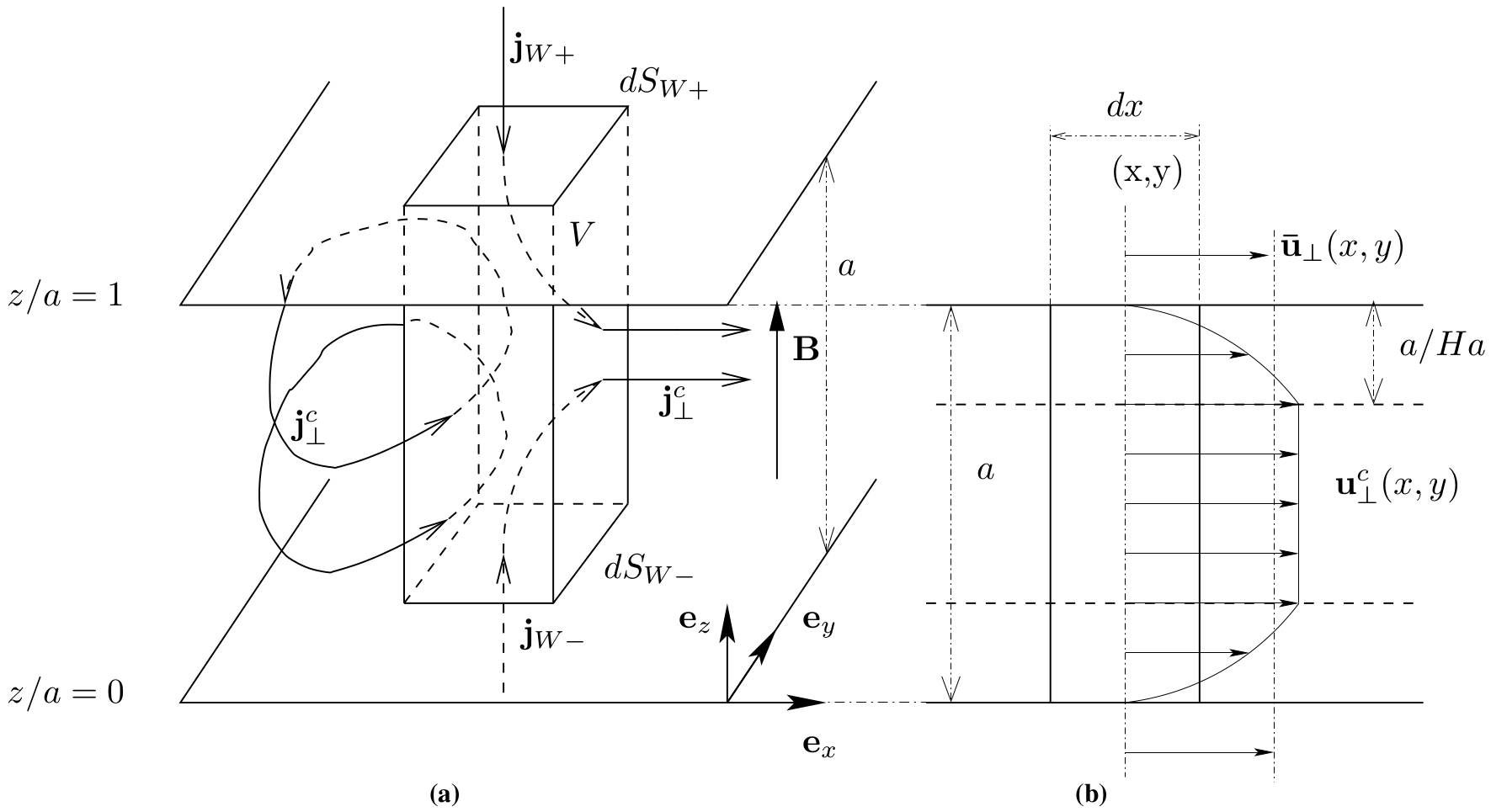
Figure 1: General flow configuration, with control surface V to which momentum conservation is applied in order to derive the general equation for 2d models (1)

Rewriting the equation derived by [21] in non-dimensional terms (normalisation by fluid depth $a$, typical velocity $U$, time $a/U$, pressure $\rho U^{2}$, shear stress $(\rho\sigma U/a)Ha$ and electric current density $\sigma BU/Ha$), we get :

$$\partial_{t}\mathbf{\bar{u}}_{\bot}+\mathbf{\bar{u}}_{\bot}.\boldsymbol{\nabla}_{\bot}\mathbf{\bar{u}}_{\bot}+\mathbf{\nabla}_{\bot}\bar{p}-\dfrac{N}{Ha^{2}}\mathbf{\nabla}^{2}_{\bot}\mathbf{\bar{u}}_{\bot}-\frac{N}{Ha}\left(\mathbf{\bar{j}}_{\bot}\times\mathbf{e}_{z}\right)=-\overline{\left(\mathbf{u}^{\prime}\mathbf{.\nabla}\right)\mathbf{u}^{\prime}}+\frac{N}{Ha}\mathbf{\tau}_{W},$$ (1)

where the over-bar denotes z-averaging across the fluid depth ($z=0$ to $z=1$). $\mathbf{u}^{\prime}$ represents the departure from the averaged velocity from the average $\mathbf{\bar{u}}$, so that the average of $\mathbf{u}^{\prime}$ is zero. Quantities averaged along $z$ are by definition dependent only on $x$ and $y$. The corresponding Nabla operator $\boldsymbol{\nabla}_{\bot}$ is two dimensional and carries the subscript ()_⊥. Similarly, the same subscript on a vector indicates components perpendicular to the magnetic field only.

The two important non-dimensional numbers mentioned in section 1 appear: the Hartmann number $Ha=aB\sqrt{\sigma/\rho\nu}$, and the interaction parameter $N=\sigma B^{2}a/(\rho U)$.

The $z$-average of the $\mathbf{u}_{\bot}\mathbf{.\nabla}_{\bot}\mathbf{u}_{\bot}$ does not reduce to $\mathbf{\bar{u}}_{\bot}\mathbf{.\nabla}_{\bot}\mathbf{\bar{u}}_{\bot}$: like in turbulence, a ”Reynolds stress” $\overline{\left(\mathbf{u}^{\prime}\mathbf{.\nabla}\right)\mathbf{u}^{\prime}}$ appears, involving the deviation $\mathbf{u}^{\prime}$ from the averaged velocity. The first term on the right hand side is effectively a Reynolds-stress term arising from the departure to the average of the velocity along the field direction $\mathbf{e}_{z}$. The non-dimensional wall stress term $\mathbf{\tau}_{W}$ is the average of stresses on the planes at $z=0$ and at $z=1$, and is dependent on the $(x,y)$ coordinates only.
At low $Rm$, the Ohm’s law is linear. The equations governing continuity of electric current and incompressibility are also linear so they may be averaged to give:

$$\begin{array}[]{cc}\boldsymbol{\nabla}.\mathbf{\bar{j}}_{\bot}=-j_{W},&\boldsymbol{\nabla}.\mathbf{\bar{u}}_{\bot}=0\\ \end{array}$$ (3)

$$\frac{1}{Ha}\mathbf{\bar{j}}=\mathbf{\bar{E}}+\mathbf{\bar{u}}\times\mathbf{e}_{z}$$ (4)

where $j_{W}$ is the current density injected at one or both of the confining planes and $\mathbf{E}$ is a non-dimensional electric field. Taking the curl of the Ohm’s law and using the incompressibility condition, one sees that $\mathbf{\bar{j}_{\bot}}$ is irrotational. It follows that there is a potential $\psi_{0}$ for $\mathbf{\bar{j}}_{\bot}$ which satisfies Poisson’s equation, the source term being $j_{W}$:

$$\begin{array}[]{cc}\mathbf{\bar{j}}_{\bot}=\mathbf{\nabla}_{\bot}\psi_{0},&\boldsymbol{\nabla}_{\bot}^{2}\psi_{0}=-j_{W}.\end{array}$$ (5)

The potential $\psi_{0}$ is determined from the current source as the solution of this Poisson equation (5), which is unique for a given current flux $\mathbf{\bar{j}}_{\bot}.\mathbf{n}$ at the lateral boundaries. Then, using the vector field $\mathbf{u}_{0}$ of streamfunction $\psi_{0}$, the Lorentz force in equation (1) turns out to depend on the boundary condition on the electric current as $\mathbf{\bar{j}}_{\bot}\times\mathbf{e}_{z}=\mathbf{u}_{0}$.

At this point, we insist that no approximation has been made on the equations of motion. The next step is to then express $\mathbf{\tau}_{W}$ and the Reynolds-stress tensor using physical models derived from asymptotic expansions performed on the full 3d equations of motion equation. We give two examples of the resulting 2d models in the next two paragraphs, which are going to be used to perform numerical simulations throughout the rest of this paper. For more detail about the derivation of these models, the reader is referred to [21].

2.2 The SM82 model

[25] were the first to construct a 2d model based on the above ideas. They used the classical Hartmann layer profile for the boundary layer model and assumed that the velocity and pressure in the core do not depend on $z$ (the 2d core model). These two assumptions are of first order in the limits $N\rightarrow\infty$ and $Ha\rightarrow\infty$, keeping the ratio $Ha/N$ finite (i.e. assuming that $Ha$ and $N$ are of comparable orders of magnitude). The Hartmann layer theory states that $\mathbf{\tau}_{W}$ is related to the excess current in the Hartmann layer with:

$$\mathbf{\tau}_{W}=n(\mathbf{\bar{j}}-\mathbf{j}^{c}_{\perp})\times\mathbf{e}_{z}=n(\mathbf{u}^{c}_{\perp}\times\mathbf{e}_{z})\times\mathbf{e}_{z}=-n\mathbf{u}^{c}_{\perp}.$$ (6)

This relates $\mathbf{\tau}_{W}$ to the core electric current $\mathbf{j}^{c}$ and velocity $\mathbf{u}^{c}$. $n$ is the number of Hartmann layers in the flow. $n=1$ if the upper plane $z=1$ is a free surface, and $n=2$ if it is a rigid wall.

To make progress with the problem expressed in terms of averages, we need to relate velocities to $\mathbf{\bar{u}}$. An important feature of the Hartmann layers in this context is that the velocity profile in the Hartmann layer is of the form $\mathbf{u}_{\perp}=\mathbf{u}^{c}f(z)$, where $f(z)=1-exp(Haz)$ is the classical Hartmann layer profile which doesn’t depend on the location $(x,y)$. It follows that the z-average velocity is proportional to the core velocity with a constant coefficient:

$$\mathbf{\bar{u}}=\mathbf{u}^{c}_{\perp}(1-n\delta^{*}),$$

where $\delta^{*}$ is the displacement thickness of each Hartmann layer and equal to $Ha^{-1}$. This simple form also implies that the friction $\mathbf{\tau}_{W}$ acts as a linear damping proportional to the velocity, with dimensional characteristic time $t_{H}=(a^{2}/\nu)(1/Ha)$. Now neglecting the Reynolds stress of order $Ha^{-1}N^{-1}$ for this particular profile, (1) yields the so-called SM82 model in non-dimensional variables:

$$(\partial_{t}+\mathbf{\bar{u}}_{\bot}.\mathbf{\nabla}_{\bot})\mathbf{\bar{u}}_{\bot}+\mathbf{\nabla}\bar{p}-\frac{N}{Ha^{2}}\mathbf{\nabla_{\bot}^{2}\bar{u}}_{\bot}=\frac{N}{Ha}(\mathbf{u}_{0}-n\mathbf{\bar{u}}_{\bot}).$$ (7)

The theoretical precision of this model is first order, i.e. an error of order $max(1/Ha,1/N)$ is expected on the velocity and pressure. In spite of its simplicity, this model is found to give good results in many well known cases such as parallel layers ([21]) but it fails to describe flows in which the traditional Hartmann layer is modified by the presence of inertial effects, such as in rotating flows for instance. The PSM2000 model described in the next section is built to overcome this weakness.

2.3 The PSM2000 model

2.3.1 General equations

In the model developed by [21], a new inertial Hartmann layer profile is derived from a second order approximation to the Navier-Stokes equations, in the limits $N\rightarrow\infty$ and $Ha\rightarrow\infty$ (still keeping the ratio $Ha/N$ finite). It incorporates inertia as a perturbation and is therefore a refinement of the SM82 model. At this order, the velocity far from the walls (i.e. $z>>Ha^{-1}$ and $1-z>>Ha^{-1}$) is still independent of $z$. The final 2d model is derived in a similar way as SM82, although it involves more tedious steps. The most obvious difference between the PSM2000 and the SM82 model is the appearance of cubic terms as well as $\partial_{t}\left(\mathbf{\bar{u}}_{\perp}.\mathbf{\nabla}_{\bot}\mathbf{\bar{u}}_{\perp}\right)$ terms. They come from the additional terms accounting for inertia in the modified Hartmann layer profile. The latter are proportional to $\mathbf{\bar{u}}_{\perp}.\mathbf{\nabla}_{\bot}\mathbf{\bar{u}}_{\perp}$ and $\partial_{t}\mathbf{\bar{u}}_{\perp}$ so that when this profile is used to evaluate the $\overline{\mathbf{u}^{\prime}.\mathbf{\nabla}\mathbf{u}^{\prime}}$ in (1), this yields the final form of the PSM2000 equations :

$$\mathbf{\nabla}_{\bot}.\mathbf{\bar{u}}_{\perp}=0$$ (8)

$$(\partial_{t}+\mathbf{\bar{u}}_{\bot}.\mathbf{\nabla}_{\bot})\mathbf{\bar{u}}_{\perp}+\mathbf{\nabla}_{\bot}\bar{p}-\frac{N}{Ha^{2}}\mathbf{\nabla}_{\bot}^{2}\mathbf{\bar{u}}_{\perp}=\frac{N}{Ha}\left(\mathbf{u}_{0}-n\mathbf{\bar{u}}_{\perp}\right)+\dfrac{n}{HaN}\left(\dfrac{7}{36}\mathcal{D}_{\mathbf{\bar{u}}_{\perp}}+\dfrac{1}{8}\partial_{t}\right)\mathbf{\bar{u}}_{\perp}.\mathbf{\nabla}_{\bot}\mathbf{\bar{u}}_{\perp}$$ (9)

where the operator $\mathcal{D}_{\mathbf{\bar{u}}_{\perp}}$ is defined as:

$$\mathcal{D}_{\mathbf{\bar{u}}_{\perp}}:\mathbf{F}\longmapsto\mathcal{D}_{\mathbf{\bar{u}}_{\perp}}\mathbf{F}=\left(\mathbf{\bar{u}_{\perp}.\nabla}_{\bot}\right)\mathbf{F}+\left(\mathbf{F.\nabla}_{\bot}\right)\mathbf{\bar{u}}_{\perp}.\\$$ (10)

Out of the two new terms which appear, compared to SM82, we are mainly interested in the one with the operator $\mathcal{D}_{\mathbf{\bar{u}}_{\perp}}$, which accounts for the effects of classical Ekman pumping when a vortex stands over a boundary layer. The advantageous feature of PSM2000, is that the effects are described locally, which allows us to determine their influence on any vorticity field. Most of the new results presented in this paper come from the study of this term.

The model is more precise than SM82, in the sense that velocity and pressure should be evaluated with an error of order $max(1/(HaN),1/N^{2},1/Ha^{2})$. In the practical cases studied thereafter, $N$ is in fact smaller than $Ha$ so that the corrections to the velocity involving $1/N$ are more important than those involving $1/Ha$. It can be shown that the terms involving $1/Ha$ merely improve the precision of the model but don’t account for any new phenomenon, as opposed to the $1/N$ terms which carry the effects of the local 3d recirculations ([21]). An analytical model for Hartmann-Bodewädt layers can be derived from the present model (for the basic theory of Bodewädt layers, see [10]). Comparison of the latter with fully non-linear simulations in the axisymmetric case has shown that (9) is satisfactorily valid if the value of the interaction parameter $N$ remains at least of the order of unity ([7]).

It should be noticed that one of the main advantages of the SM82 and PSM2000 models is that both rely on asymptotic expansions performed on the Navier-Stokes equation without any kind of empirical parameter, which allows us to quantify their precision using non dimensional numbers $N^{-1}$ and $Ha^{-1}$.

2.3.2 Effect on the vorticity field

We shall now characterise the PSM2000 model by showing how the local recirculations it accounts for affect the vorticity field. The first step consists in deriving the equation satisfied by the average vorticity $\omega\mathbf{e}_{z}=\nabla\times\mathbf{\bar{u}}_{\perp}$ from the 2d model (9). This equation is obtained by taking the curl of (9), and using the identity $\mathcal{D}_{\mathbf{\bar{u}}_{\perp}}\mathbf{F=\nabla}_{\bot}\left(\mathbf{\bar{u}_{\perp}.F}\right)-\mathbf{\bar{u}_{\perp}\times\nabla}_{\bot}\times\mathbf{F-F\times\nabla}_{\bot}\times\mathbf{\bar{u}}_{\perp}$, as well as $\mathbf{\nabla}_{\bot}.\omega\mathbf{e}_{z}=0$ :

$$(\partial_{t}+\mathbf{\bar{u}}_{\perp}.\nabla)\omega-\frac{N}{Ha^{2}}\nabla_{\bot}^{2}\omega=-\frac{N}{Ha}\left(\omega_{0}-n\alpha\omega\right)\mathbf{+}\\ \tfrac{7}{36}\tfrac{n}{HaN}\left(\left[\mathbf{\bar{u}}_{\perp}.\mathbf{\nabla}_{\bot}\mathbf{\bar{u}}_{\perp}\right]\mathbf{.\nabla}_{\bot}\omega+\left(\mathbf{\bar{u}}_{\perp}.\mathbf{\nabla}_{\bot}\right)\left(\mathbf{\bar{u}}_{\perp}.\nabla_{\bot}\omega\right)+\omega\mathbf{\nabla}_{\bot}.\left[\mathbf{\bar{u}}_{\perp}.\mathbf{\nabla}_{\bot}\mathbf{\bar{u}}_{\perp}\right]\right)+\tfrac{1}{8}\tfrac{n}{HaN}\partial_{t}\left(\mathbf{\bar{u}}_{\perp}.\mathbf{\nabla}_{\bot}\omega\right)$$ (11)

The additional terms are direct consequences of the secondary flows : as the non-linear terms in the expression of the velocity profile in the inertial Hartmann layers are proportional to $\mathbf{\bar{u}}_{\perp}.\mathbf{\nabla}_{\bot}\mathbf{\bar{u}}_{\perp}$ and $\partial_{t}\mathbf{\bar{u}}_{\perp}$, the $\left[\mathbf{\bar{u}}_{\perp}.\mathbf{\nabla}_{\bot}\mathbf{\bar{u}}_{\perp}\right]\mathbf{.\nabla}_{\bot}\omega$ and $\partial_{t}\mathbf{\bar{u}}_{\perp}.\mathbf{\nabla}_{\bot}\omega$ terms represent the amount of vorticity conveyed to the point $\left(x,y\right)$ from its neighbourhood by secondary flows, while the $\left(\mathbf{\bar{u}}_{\perp}.\mathbf{\nabla}_{\bot}\right)\left(\mathbf{\bar{u}}_{\perp}.\boldsymbol{\nabla}_{\bot}\omega\right)$ terms represent the transport of vorticity due to these recirculations being carried by the main flow. The inertial model of the Hartmann layer also predicts a vertical velocity proportional to $\mathbf{\nabla}_{\bot}.\left[\mathbf{\bar{u}}_{\perp}.\mathbf{\nabla}_{\bot}\mathbf{\bar{u}}_{\perp}\right]$ at the edge of the layer. The $\omega\mathbf{\nabla}_{\bot}.\left[\mathbf{\bar{u}}_{\perp}.\mathbf{\nabla}_{\bot}\mathbf{\bar{u}}_{\perp}\right]$ expression is a source term related to the vorticity created in the core by this phenomenon.

The next step is to seek the effects of the non linear terms of (11) on a vortex spot sketched as a local extremum of vorticity. We assume that the vorticity field exhibits a local extremum and that this extremum is conveyed by a background flow $V\mathbf{e}_{x}$. The extremum is thus located at the point $\left(x_{0}+Vt,y_{0}\right)$ i.e. :

$$\partial_{x}\omega\left(x_{0}+Vt,y_{0}\right)=\partial_{y}\omega\left(x_{0}+Vt,y_{0}\right)=0\\$$ (12)

In addition, the background flow $V\mathbf{e}_{x}$ is considered constant and large in front of the local velocity variations:

$$\mathbf{\bar{u}}_{\perp}=V\mathbf{e}_{x}+\mathbf{v}^{\prime}\left(x,y,t\right)$$ (13a)

$$\partial_{x}V\left(x,y,t\right)=\partial_{y}V\left(x,y,t\right)=\partial_{t}V\left(x,y,t\right)=0$$ (13b)

$$\left\|\mathbf{v}^{\prime}\left(x,y,t\right)\right\|\ll V$$ (13c)

so that the local velocity $\mathbf{v}^{\prime}\left(x,y,t\right)=v_{x}\mathbf{e_{x}}+v_{y}\mathbf{e_{y}}$ satisfies the conservation equation:

$$\mathbf{\nabla}_{\bot}.\mathbf{v}^{\prime}=0$$ (14)

The extremum condition (12) implies that the transport by secondary flows doesn’t act:

$$\left[\mathbf{\bar{u}}_{\perp}.\mathbf{\nabla}_{\bot}\mathbf{\bar{u}}_{\perp}\right]\mathbf{.\nabla}_{\bot}\omega\left(x_{0}+Vt,y_{0}\right)=0.\\$$ (15)

Expanding $\omega\mathbf{\nabla}_{\bot}.\left[\mathbf{\bar{u}}_{\perp}.\mathbf{\nabla}_{\bot}\mathbf{\bar{u}}_{\perp}\right]\left(x_{0}+Vt,y_{0}\right)$ and $\left(\mathbf{\bar{u}}_{\perp}.\mathbf{\nabla}_{\bot}\right)\left(\mathbf{\bar{u}}_{\perp}.\boldsymbol{\nabla}_{\bot}\omega\right)\left(x_{0}+Vt,y_{0}\right)$ in terms of the derivatives of $\omega$ and $\mathbf{v}^{\prime},$ and using (12), (13b) and (14) yields:

$$\omega\mathbf{\nabla}_{\bot}.\left[\mathbf{\bar{u}}_{\perp}.\mathbf{\nabla}_{\bot}\mathbf{\bar{u}}_{\perp}\right]\left(x_{0}+Vt,y_{0}\right)=2V^{2}\partial_{xx}^{2}\omega+\omega\left[2\left(\partial_{x}v_{x}^{\prime}\right)^{2}+\left(\partial_{x}v_{y}^{\prime}\right)^{2}+\left(\partial_{y}v_{x}^{\prime}\right)^{2}-\omega^{2}\right].$$ (16a)

$$\left(\mathbf{\bar{u}}_{\perp}.\mathbf{\nabla}_{\bot}\right)\left(\mathbf{\bar{u}}_{\perp}.\boldsymbol{\nabla}_{\bot}\omega\right)\left(x_{0}+Vt,y_{0}\right)=V^{2}\partial_{xx}^{2}\omega+2V(\partial_{x}\mathbf{v}^{\prime}).\boldsymbol{\nabla}_{\bot}\omega++V\mathbf{v}^{\prime}.\boldsymbol{\nabla}_{\bot}\partial_{x}\omega+\mathbf{v}^{\prime}.\boldsymbol{\nabla}_{\bot}(\mathbf{v}^{\prime}.\boldsymbol{\nabla}_{\bot}\omega).$$ (16b)

Using the relation $\partial_{t}=V\partial_{x}$ for the advected extremum, the unsteady term can be rewritten as:

$$\partial_{t}\left(\mathbf{\bar{u}}_{\perp}.\mathbf{\nabla}_{\bot}\omega\right)\left(x_{0}+Vt,y_{0}\right)=V^{2}\partial^{2}_{xx}\omega+V(\partial_{x}\mathbf{v}^{\prime}).\boldsymbol{\nabla}_{\bot}\omega+V\mathbf{v}^{\prime}.\boldsymbol{\nabla}_{\bot}\partial_{x}\omega.$$ (17)

The condition (13c) ensures that the terms proportional to $V^{2}$ in the r.h.s. of (16a), (16b) and (17) are arbitrarily larger than the others. Then $\omega\mathbf{\nabla}_{\bot}.\left[\mathbf{\bar{u}}_{\perp}.\mathbf{\nabla}_{\bot}\mathbf{\bar{u}}_{\perp}\right]\left(x_{0}+Vt,y_{0}\right)\simeq 2V^{2}\partial_{xx}^{2}\omega$, $\left(\mathbf{\bar{u}}_{\perp}.\mathbf{\nabla}_{\bot}\right)\left(\mathbf{\bar{u}}_{\perp}.\boldsymbol{\nabla}_{\bot}\omega\right)\left(x_{0}+Vt,y_{0}\right)\simeq V^{2}\partial_{xx}^{2}\omega$ and $\partial_{t}\left(\mathbf{\bar{u}}_{\perp}.\mathbf{\nabla}_{\bot}\omega\right)\left(x_{0}+Vt,y_{0}\right)\simeq V^{2}\partial_{xx}^{2}\omega$ so that the non linear term acts on the vorticity as an anisotropic diffusion, in the direction of the background velocity, with related diffusivity:

$$\eta=\frac{17n}{24}\frac{Ha}{N_{V}^{2}}\nu$$ (18)

where, $N_{V}$ is the interaction parameter based on the average flow $V$. This confirms that the additional terms are dissipative, as shown by [9]. The related diffusivity can also be seen as a turbulent diffusivity which is determined the by secondary flows. This extends the analogy with the usual turbulent Reynolds stresses which are sometimes interpreted as a turbulent diffusion with related ”eddy viscosity”.

The main result of this section is that any elementary vortex of the flow is spread by nonlinearities, so that the latter have a smoothing effect on the whole velocity field. This is to be related to the results of the numerical simulations presented in section 5. Also, [9] showed that the non-linear terms in (9) induce a diffusion along streamlines for small amplitude waves. He also showed that PSM2000 shares this feature with the model proposed by [4] for two-dimensional turbulence based on ideas from the Anticipated Vorticity Method of [3]. This model features additional non linear terms like PSM2000 and describes well some oceanic and atmospheric flows. This suggests that accounting for the 3d recirculations in oceans and atmospheres could lead to accurate 2d models similar to PSM2000.

3 Numerical setup

3.1 The numerical model

We use the finite volume code FLUENT/UNS featuring a second order upwind spatial discretisation. The cases studied are unsteady and the time-scheme is a second order implicit pressure-velocity formulation. Within each iteration, equations are solved one after the other (segregated mode) using the PISO algorithm proposed by [12]. In short, PISO is a predictor-corrector method which substantially reduces the number of iterations per time step, especially in unsteady calculations, by decomposing each iteration into one prediction step and several (two here) correction steps: in the prediction step, a first (predicted) velocity field is obtained by solving the momentum equations in which the value of the pressure is taken from the result of the previous iteration (the equations are then implicit for the velocity but explicit for the pressure). In the next step, a corrected pressure is obtained by solving an explicit Poisson equation, in which the velocity is the result from the prediction step. A second (corrected) velocity field is solution of the momentum equations in which inertial terms are evaluated using the velocity obtained in the prediction step and in which the pressure is the corrected one. This last step (called correction) is iterated one additional time. Note that this algorithm is in fact a modified version of the one described by [12] in which the prediction-correction is applied in between time steps rather than in between iterations within the same time step.
The additional terms in (9) are modelled the following way:

• The Hartmann friction $-\mathbf{\bar{u}}_{\perp}/t_{H}$ is expressed implicitly, i.e. as $-\mathbf{\bar{u}}^{(n+1)}_{\perp}/t_{H}$ at current time $t^{(n+1)}$, where $\mathbf{\bar{u}}^{(n+1)}_{\perp}$ is the velocity variable at the current time step, on which the PISO iterations are performed.

• The $\mathbf{\bar{u}}_{\perp}\boldsymbol{\nabla}_{\bot}.\mathbf{\bar{u}}_{\perp}$ terms appearing in the PSM2000 model additional terms and their gradients are treated implicitly in time and updated at the end of each iteration within the time steps, using the latest values of the velocity obtained from the resolution of the pressure-velocity equations by the PISO algorithm. These terms are therefore not modified during the PISO iterations.

• The additional time derivative is second order implicit, i.e. expressed at time $t^{(n+1)}$ as $[\partial_{t}(\mathbf{\bar{u}}_{\perp}.\boldsymbol{\nabla}_{\bot})\mathbf{\bar{u}}_{\perp}]_{t^{(n+1)}}=\frac{1}{2\Delta t}\left(3[(\mathbf{\bar{u}}_{\perp}.\boldsymbol{\nabla}_{\bot})\mathbf{\bar{u}}_{\perp}]_{t^{(n+1)}}-4[(\mathbf{\bar{u}}_{\perp}.\boldsymbol{\nabla}_{\bot})\mathbf{\bar{u}}_{\perp}]_{t^{(n)}}+(\mathbf{\bar{u}}_{\perp}.\boldsymbol{\nabla}_{\bot})\mathbf{\bar{u}}_{\perp}]_{t^{(n-1)}}\right)$, where the superscripts $(n)$ and $(n-1)$ refer to the variables taken from the two previous time steps.

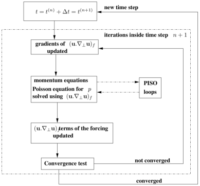
Figure 2: Algorithm used to solve the equation (9) numerically. $(\mathbf{u}.\boldsymbol{\nabla}_{\bot}\mathbf{u})_{f}$ represents the inertial terms appearing in the additional terms of PSM2000.

A summary of the algorithm is sketched in figure 2.

3.2 Tests on the numerical model

We shall now investigate the ability of the numerical system to solve equations (9). To this end, we perform a convergence study under grid refinement toward an analytical solution. As these equations are both new and complex, no exact analytical solution has been exhibited up to now. We therefore follow the procedure recommended by [23] which consists in specifying an analytical velocity field and adjusting the forcing term (here $\mathbf{u}_{0}$ in (9)) so that the specified field is solution of the equations. We choose the case of a flow confined between two co-rotating vertical cylinders (respective radius $r_{int}$ and $r_{ext}$) and two horizontal plates (at $z=0$ and $z=1$), plunged in a vertical uniform magnetic field. Equations (9) then apply on the 2d annulus $r_{int}<r<r_{ext}$. The parameters $r_{int}$, $r_{ext}$, $Ha$ and $N$ can be set for the solution to exhibit a significant Ekman pumping, which is the very kind of phenomenon the PSM2000 model is supposed to account for. The reference solution consists in an azimuthal wave superimposed on a $1/r^{2}$ axisymmetric radial profile. Numerical constants are adjusted so that the wave amplitude is $10\%$ of the azimuthal velocity at the inner cylinder, and so that the velocity is tangent to the walls located at $r=r_{int}$ and $r=r_{ext}$:

$$\frac{v_{\theta}(r)}{v_{\theta}(r_{int})}=\frac{r^{2}_{int}}{r^{2}}+0.407(r-r_{int})(r-r_{ext})(r-\frac{r_{int}+r_{ext}}{2})cos(7\theta+3.5t)$$

$$\frac{v_{r}(r)}{v_{\theta}(r_{int})}=\frac{2.4929}{r}(r^{2}_{int}r^{2}_{ext}-2rr_{int}r_{ext}(r_{int}+r_{ext})+r^{2}(r^{2}_{int}+r^{2}_{ext}+4r_{int}r_{ext}-$$

$$2r^{3}(r_{int}+r_{ext})+r^{4})sin(7\theta+3.5t)$$ (19)

The initial conditions at $t=0$ and the Dirichlet boundary conditions at the walls for the velocity are chosen to match (19). These conditions avoid the occurrence of a boundary layer along the cylinders for which no analytical solution would be known. Setting $Ha=111$, $N=12$ ($N$ is built using $v_{\theta}(r_{int})$ and $r_{ext}/r_{int}=10$ ensures that the region $r_{ext}-r<<r_{ext}$ is dominated by viscosity while non-linear terms dominate the dynamics near the inner cylinder $r_{int}-r<<r_{int}$). The convergence tests are performed on a structured mesh with twice as many azimuthal nodes as along one radius. The time steps are adjusted to satisfy the Courant-Friedrich-Lewy condition for the maximal azimuthal phase velocity of the imposed wave (resp. 0.018 s, 0.0128 s, 0.009 s, 0.007 s for cases with resp. 50, 70, 100 and 140 radial modes). Each calculation runs over a full time-period of the imposed solution. Figure 3 shows that the $\mathcal{L}_{2}$ norm of the relative error over the domain decreases approximately as $n_{cell}^{-0.64}$ where $n_{cell}$ is the number of elements in the mesh. This confirms the reliability of the numerical system. It is however important to notice that the convergence is not of second order spatial accuracy, although all quantities are being discretised at this order. The reason for this precision loss is that the $\mathcal{D}_{\mathbf{\bar{u}}_{\perp}}\mathbf{\bar{u}}_{\perp}.\mathbf{\nabla}_{\bot}\mathbf{\bar{u}}_{\perp}$ terms appearing in (9) are calculated by taking the gradient of the $\mathbf{\bar{u}}_{\perp}.\boldsymbol{\nabla}_{\bot}\mathbf{\bar{u}}_{\perp}$ variables. Although these variables are known to second order precision, the resulting gradients are not. The achieved accuracy is however sufficient for our purpose, which is to model physical experiments rather than to build a refined numerical model. Such a refined numerical work based on the PSM2000 model can be found in [9].

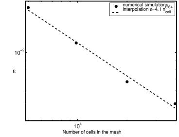
Figure 3: Time average of the $\mathcal{L}_{2}$ norm of the relative error $\epsilon=\|U_{numeric}-U_{ref}\|_{2}/\|U_{ref}\|_{2}$ in numerical simulations, compared to the reference analytical solution (19) versus number of cells in the mesh.

4 Simulation of the free decay of isolated vortices generated by a single-electrode

4.1 Experimental device of reference

In the next two sections, we shall use the numerical implementation of both PSM2000 and SM82 described in the previous section to recover the results of two MHD experiments, which couldn’t be modelled by classical theories. We first perform the simulations on [24] ’s electrically driven vortices using PSM2000 only. The experimental setup consists in a cylindrical tank (diameter $2R=120$ mm) filled with mercury (depth $a=19.2$ mm) with an insulating bottom plate, an upper free surface ($n=1$) and an electrically conducting circular wall at $r=R$ (see figure 4). Electric current is injected into the mercury via a small electrode (diameter $2r_{e}=2.5$ mm) located in the bottom plate. The injected current $j_{W}$ can be approximated as a Dirac-delta function centred at the edge of the electrode $r=r_{e}$, with integral equal to the total injected current $I$: $j_{W}=I/(2\pi r_{e})\delta(r-r_{e})$. The corresponding forcing is azimuthal and given from the solution of (5) which yields:

$$\forall r>r_{e},\mathbf{u}_{0}=-\dfrac{B}{\rho a}\dfrac{I}{2\pi r}t_{H}\mathbf{e}_{\theta}.$$ (20)

The forcing is applied until a steady regime is reached. This flow is quite stable and remains laminar. At the end of the run, the forcing is switched off and the flow decays by Hartmann friction. The experimental parameters are summarised in the table below with the corresponding non-dimensional parameters and numerical time-steps. (We give here the values of $N_{c}=N/\sqrt{Ha}$, which is scaled on the vortex core thickness of order $aHa^{-1/2}$, as [24] noticed that it is the relevant parameter that governs the recirculating effects in the vortex):

$B/$T	0.0575	0.115	0.23	0.48
$Ha$	28.41	56.82	113.6	237.2
$t_{H}$/s	110.9	55.45	27.72	13.28
$N_{c}$ ($I=50$ mA)	0.017	0.034	0.068	0.14
$N_{c}$ ($I=12.5$ mA)				0.569
$N$ ($I=50$ mA)	0.091	0.256	0.724	2.16
$N$ ($I=50$ mA)				8.76
time step /s ($I=50$ mA)	0.043	0.065	0.076	0.080
time step /s ($I=12.5$ mA)				0.086

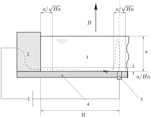
Figure 4: Experimental device of Sommeria’s vortex study: cross section of the circular tank with a schematic representation of the current supply. A typical current streamline passing through the Hartmann layer is also represented (dashed). 1: mercury, 2: electrically conducting side wall, 3: electrode for current injection, 4: electrically insulating bottom wall.

4.2 Mesh and boundary conditions

The mesh is made of quadrilateral elements, unstructured for $r<1.64$ mm and structured for $1.64$ mm$<r<R$. The radial resolution is 105 points, 25 of which are devoted to the boundary layer located at $r=R$. These points are spread in the layer according to a geometric sequence of ratio 1.3 starting at $r=R$ with an initial interval of $5.10^{-6}$ mm. The azimuthal resolution is of 150 points. The time step is chosen so that the related cutoff frequency matches the spatial cutoff frequency for the maximal flow velocity (Courant-Friedrich-Lewy condition). Values are given in the table above. The usual no-slip condition at the wall $r=R$ is applied.

4.3 Free decay

Figure 5 shows the decay of electric resistance between the central electrode and the conductive side wall. This quantity is derived in [24] from the velocity field as $\mathcal{R}=(\tilde{\psi}_{wall}-\tilde{\psi}_{electrode})/I=-1/(IB)\int_{b}^{R}u_{\theta}dr$, (where $\tilde{\psi}$ is the dimensional electric potential) using the fact that there is no current outside the Hartmann layer because the flow is two-dimensional. The numerical simulations from the model show that $\mathcal{R}$ decays strongly at early times, and the decay rate then stabilises around $(0.9t_{H})^{-1}$. This agrees very well with the experiment. Also, the small discrepancy between PSM2000 and the experiment increases with $N_{c}^{-1}$. This is precisely what one should expect as PSM2000 is derived from asymptotic expansions on $Ha^{-1}$ and $N^{-1}$. This tends to confirm that these non-dimensional parameters provide a good measure of the precision of the model.

Physically, the strong damping at early times - weaker for weak currents and strong fields - is explained by the presence of Ekman recirculations. Indeed, Ekman pumping induces a centrifugal flow in the core flow as well as a centripetal flow in the Hartmann layers. The mass conservation requires that the vertically integrated mass fluxes related to these two radial flows be the same. As the velocity is smaller in the Hartmann layer, the net effect of Ekman pumping is a centrifugal transport of angular momentum. This has two consequences: The first one is that the wall side boundary layer is squeezed by this transport so that the wall friction is increased. The recirculations are important when the vortex still rotates fast, so that angular momentum is conveyed toward the side layer, which increases dissipation and enhances the damping. This phenomenon is however not very strong in the present case since the velocities near the lateral wall are rather small, as opposed to the MATUR case described in section 5.
When the flow has been significantly damped, the Ekman recirculation disappears and the wall side layer goes back to its typical $Ha^{-1/2}$ thickness so that the associated dissipation becomes small compared to the Hartmann damping. The decay rate of the velocity then matches approximately the $t_{H}^{-1}$ value predicted by the linear theory. The second consequence is that azimuthal velocities initially decrease much faster for points which are closer to the centre as shown in figure 6. The reason is that the recirculations arise from centripetal jets in the Hartmann layer, which are therefore stronger at the centre of the tank. This also explains that recirculations tend to noticeably ”broaden” the vortex core, as measured by [24] and confirmed theoretically by [21].

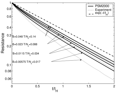
Figure 5: Time-decay of the resistance between the central electrode and the side wall for several magnetic fields (injected current before decay is $I=0.05$ A unless otherwise specified). Resistances are normalised by their value at equilibrium, at the moment the forcing is switched off ($t=0$ on the graphs). The exponential decay is the one predicted by the SM82 model.

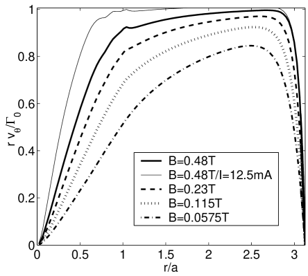
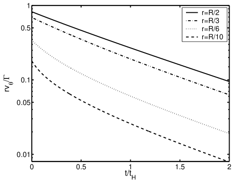
Figure 6: Angular momentum normalised by $\Gamma_{0}=I/(2\pi(\rho\sigma\nu)^{1/2})$. The radial profiles of angular momentum (top) are obtained numerically and show that the main effect of the recirculations is to broaden the vortex core. Injected current before decay is $I=0.05$ A unless otherwise specified. Time-decay of azimuthal velocity for different radial positions (bottom), just after the forcing is switched off (referred to as $t=0$ here), obtained from the numerical simulations of the PSM2000 model at B=0.23 T. Secondary flows are stronger at the centre, where the velocity decays faster.

5 Numerical Simulations for the MATUR experimental setup

5.1 Experimental device of reference

We now come to the main part of this work, where PSM2000 and SM82 are both compared and used to recover and explain the results obtained by [2] with the MATUR (MAgnetic TURbulence) experimental setup developed in Grenoble. MATUR is a cylindric container (diameter $2R=0.22$ m) with an electrically insulating bottom and conducting vertical walls (figure 7). Electric current is injected at the bottom through a large number of point-electrodes regularly spread along a circle the centre of which is on the axis of the cylinder. It is filled with mercury ($a=1$ cm depth) and the whole device is placed in a steady uniform vertical magnetic field. The injected current leaves the fluid through the vertical wall inducing radial electric current lines and gives rise to and azimuthal force on the fluid included in the annulus between the electrode circle and the outer wall.

The forcing is similar to the case of section 4 but the radius where the current is injected $r_{e}=0.093$ mm is much larger so that a free shear layer is produced with a vorticity sheet at $r=r_{e}$. Instability is associated with this vorticity extremum. By contrast, in the case of section 4, the vorticity extremum was at the centre of the tank, leading to a stable flow.

The annulus of fluid $r\in[r_{e},R]$ rotates and gives rise to a concave parallel wall side layer along the outer wall ($r=R$) and a free parallel shear layer at $r=r_{e}$. The upper surface is rigid so that two Hartmann layers (at the top and the bottom) are present ($n=2$ ).
The field is $B=0.17$ T (i.e. $Ha=45.14$) and the fluid is at rest at the initial state $t=0$. Numerical simulations are performed for a total injected current $I$ in the range $[3$ A$,30$ A$]$. An approximate azimuthal velocity $U_{sm82}=I/(2\pi R\sqrt{\sigma\rho\nu})$ and associated global angular momentum per unit of height $L_{sm82}=U_{sm82}\pi R(R^{2}-re^{2})$ can be derived from the theory from [25] (see [21]), the order of magnitude of which remains valid within the framework of PSM2000. The relevant interaction parameter is scaled on the horizontal length $N_{2d}=\sigma B^{2}R/(\rho U_{sm82})$. The horizontal velocity $U_{sm82}$ is used for convenience, but this is an overestimate, so that the physical interaction parameter should be somewhat higher than $N_{2d}$.

$I$ /A	3	10	20	30
$U_{sm82}$ /m/s	0.054	0.18	0.36	0.54
$N_{2d}$	4.6	1.4	0.67	0.47
time step /s	0.025	0.01	0.01	0.007

A more comprehensive description of the experimental device and results can be found in [2].

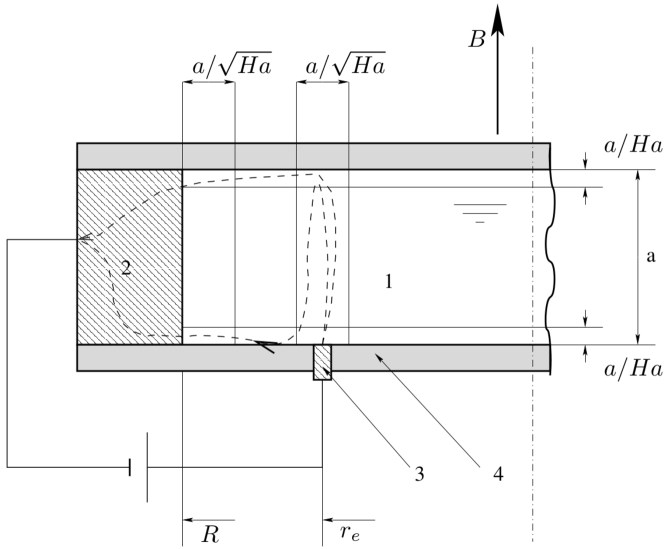
Figure 7: Radial section of the MATUR experimental setup. Some typical current streamlines passing through the Hartmann layers are also represented (dashed). 1: mercury, 2: electrically conducting side wall, 3: current injection electrode, 4: electrically insulating bottom wall.

5.2 Numerical setup

As the geometry is similar to that of Sommeria’s experiments described in section 4, we use the same mesh and the same boundary conditions at the wall located at $r=R$. This mesh ensures that the wall side layer located at $r=R$ is always described by at least 12 points. In order to reduce the CPU time, the free shear layer located at $r=r_{e}$ is not finely meshed. Indeed, the latter is thin in laminar regime (thickness $aHa^{1/2}$) which only happens in the first few seconds of each case (out of more than one minute duration of the real experiment). The layer then quickly destabilises and is replaced by large vortices with relatively smooth velocity gradients which do not require mesh refinement. This simplification might make the modelled layer slightly more unstable than the real one but does not significantly affect the quasi-steady state we are mostly interested in. As in section 4, The time step is chosen to satisfy the Courant-Friedrichs-Lewy condition, so that the temporal cutoff frequency matches the spatial cutoff frequency (see table 5.1).
All time-averaged values are calculated in the steady regime reached after a time of $3t_{H}$. The statistics are then performed over a period of $t_{H}$.

5.3 Overview of the simulated flow

The electric current is injected at $t=0$ and remains constant during the whole simulation. After a few seconds, the azimuthal velocity of the external annulus reaches the critical value that destabilises the circular free shear layer located at $r_{e}=0.093m$. This Kelvin-Helmholtz instability then produces small cyclonic vortices, merging into bigger ones (see figure 9).

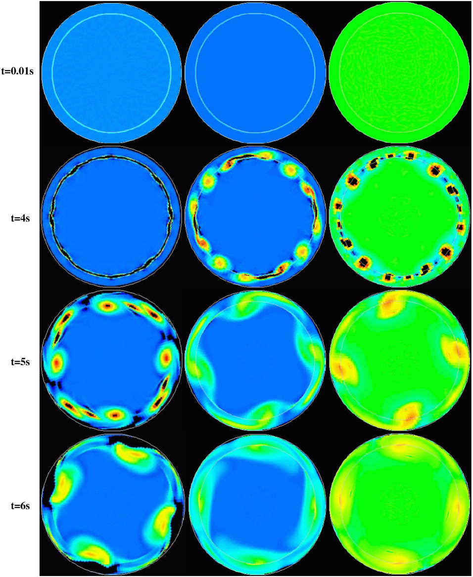
Figure 8: See caption on figure 9.

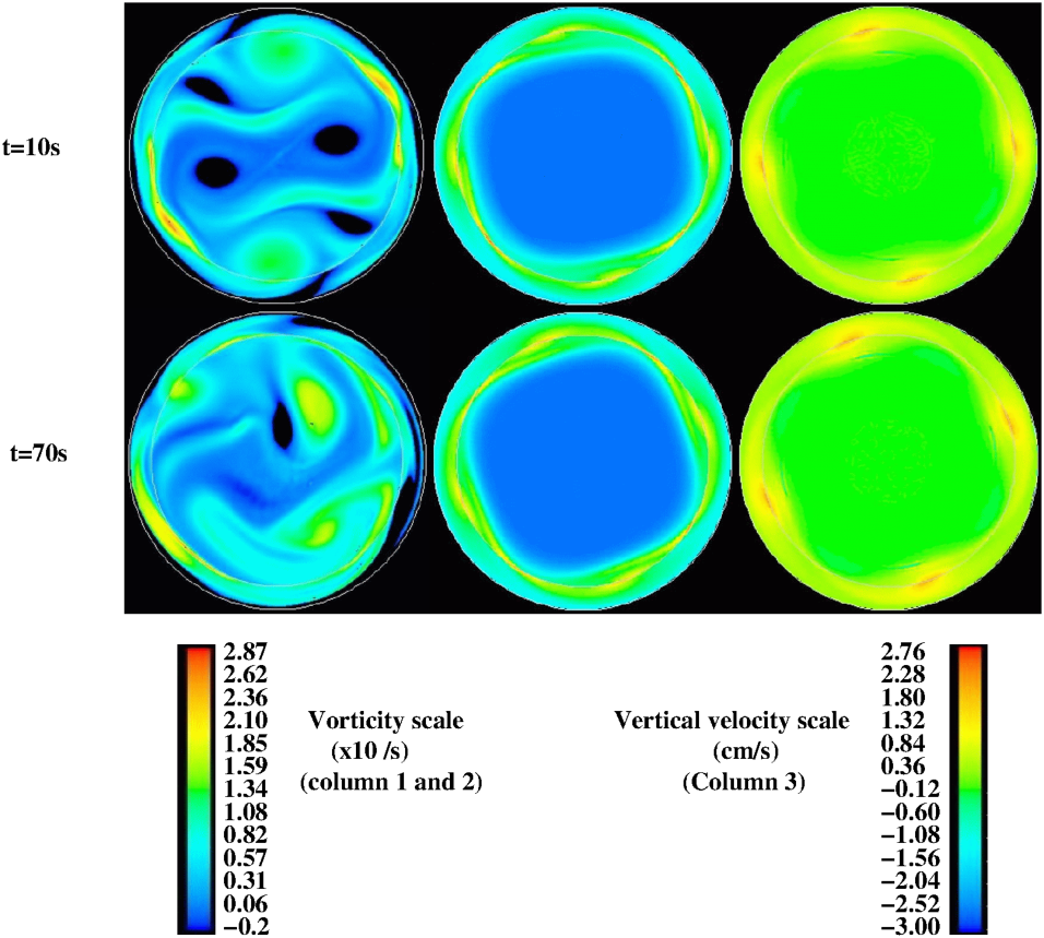
Figure 9: Evolution of the flow with time from numerical simulations for $I=30$ A, and $B=0.17$ T. Left column: vorticity fields obtained using SM82, central column: vorticity fields obtained using PSM2000. Right Column: vertical velocity fields at the edge of the Hartmann layer, computed from the horizontal velocity field given by the simulation of (9).

For low injected currents (a few Ampères), SM82 and PSM2000 predict flows which are very close to each other, but for higher values of $I$, the rotation becomes faster and Ekman pumping becomes important. As a first effect, the vorticity structures elongate in the direction of the mean flow (see figure 10$,I=30$ A) in the simulations of the PSM2000 model. Notice that this effect does not affect the pressure field directly. When the phenomenon is strong enough, vortices cannot move within the rotating reference frame anymore, so that the final state predicted by the PSM2000 model is made of a few azimuthally elongated vortices nearly in solid body rotation. For the same current, the SM82 model predicts a higher rotation speed and a much more chaotic flow, involving circular vortices of different sizes merging into one another. According to the results obtained using SM82, boundary layer separations also appear for $I=30$ A, at the side wall, which lead to the injection of big anticyclonic vortices in the flow (These vortices appear as black patches in the pictures of the left column in figures 9 and 10). The lifetime of such vortices is of the order of magnitude of the inertial time. This first view indicates clearly that the smoothing property of the PSM2000 model shown in section 2.3.3 can drastically stabilise the flow, to the point of literally suppressing turbulence. We shall now examine the results more quantitatively.

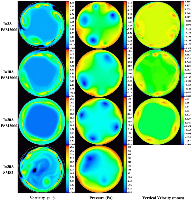
Figure 10: Quasi-steady states of the flow for $B=0.17$ T for different values of the injected current, obtained from numerical simulations. Left column : vorticity field, central column : pressure field. Right column : vertical velocity field at the edge of the Hartmann layer. The dark areas surrounded by blue colour in the vorticity field represent negative vorticity (off colorscale). Separation of the boundary layer located at the side wall surrounding the flow clearly appears for $I=3$ A (PSM2000) and $I=30$ A (SM82).

5.4 Mean velocity profiles

5.4.1 Core flow

Figure 11 shows the radial profiles of the RMS of the azimuthal velocity obtained by numerical simulations based on the SM82 and PSM2000 models and by the experiment of [2] respectively. SM82 overestimates the velocity as soon as $I$ reaches approximately $20$ A, whereas PSM2000 remains in fairly good agreement with experimental results. The latter however slightly underestimates the velocity in the inner annulus, near the injection electrodes at $r_{e}$. As a consequence, the inner half of the free shear layer is a bit thinner than in the experiments. A more crucial difference is that the SM82 model predicts a wall side layer of thickness $aHa^{-1/2}$ (which corresponds to the linear parallel layer theory. See for instance [17]), and which therefore does not depend on $I$, whereas the radial outward angular momentum transport associated to secondary flows, squeezes the wall side layer dramatically in the results obtained using the PSM2000 model (see section 5.6).

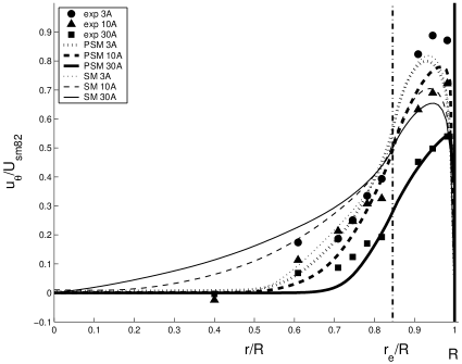
Figure 11: Azimuthal velocity profiles at quasi steady state for $B=0.17$ T (averaged on time at quasi-steady state), for several values of the injected current.

5.4.2 Squeezed wall side layers

The vertical velocity at the interface between the Hartmann layer and the core (for a mathematically rigorous definition of this interface, see [22]) is computed from the solution of the numerical simulation, using the expression for $w(z=0)$ provided by the PSM2000 model (see [21]): $w(z=0)=-(5/6)(a^{3}/\nu)(1/Ha^{3})\mathbf{\nabla}_{\bot}\mathbf{.}\left[\left(\mathbf{\bar{u}}_{\bot}\mathbf{.\nabla}_{\bot}\right)\mathbf{\bar{u}}_{\bot}\right]$. Figure 12 shows that a strong Ekman pumping occurs in the rotating annulus ($r_{e}<r<R$). The small oscillation appearing in the profile at $r\simeq r_{e}$ indicates that each big vortex conveyed by the mean flow is subject to a small Ekman pumping which is added to the global recirculation. This induces an additional radial flow. As the vertical velocity is oriented toward the core in the whole flow, mass conservation is satisfied thanks to a strong vertical jet occurring at the wall side layer, the latter being indeed the only area in the flow where $w(z=0)\leq 0$.
Also, the boundary layer at $r=R$ is squeezed by recirculations as shown in figure 13. The mechanisms which explains it is the same as for isolated vortices described in section 4.3.

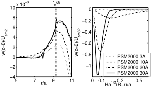
Figure 12: Time average at quasi-steady state of the radial profiles of vertical velocity at the edge of the Hartmann layer, on a whole radius (left: radial position is normalised by $a$) and within a modified wall-side layer (right: velocities are plotted versus the distance to the side wall normalised by the parallel layer thickness in linear regime).

As a consequence, the flow injected in the core outside of the wall side layer loops back to the Hartmann layers on a reduced horizontal area. This makes the already high vertical velocity maximum (oriented toward the Hartmann layers) in the wall side layer even higher, as shown on figure 12.

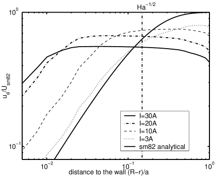
Figure 13: Radial profiles of azimuthal velocity within the wall side layer (averaged in time at quasi-steady state). Velocities are normalised by $U_{sm82}$. This graph clearly shows that the higher the forcing, the thinner the boundary layer and the more the maximum velocity is reduced, compared to flows where recirculations are neglected (which would have a maximum velocity closer to $U_{sm82}$). The smooth solid line represents the exponential profile obtained analytically from the SM82 model under the assumption of axisymmetry (typical thickness $Ha^{-1/2}$). Remark: The actual numerical computations always rely on at least 10 points to resolve the wall side boundary layer. The apparent lack of precision on the graph is a simple post-processing issue.

Figure 13 shows the dramatic thinning of the side boundary layer. Under the assumption of axisymmetry, the PSM2000 model predicts a thickness of $(36/7)(N/Ha)Rn^{3/2}$ (here $n=2$) for the parallel layer at the side wall (see [21], section 4), which is far thinner than the $aHa^{-1/2}$ thickness of linear parallel layers. This result however doesn’t apply directly here, as it ignores the extra recirculations induced by local vortices mentioned in this section. It is however noteworthy that the modified layer keeps an exponential shape, as assumed by [21] in order to derive the layer thickness in the axisymmetric case. We shall now see that the phenomenon of wall side layer thinning is much more significant in MATUR than in the case of Sommeria’s vortices (see section 4) as it reaches a point where it significantly alters the global dissipation.

5.5 Effect of the secondary flows on global quantities

5.5.1 Quasi-steady state

The direct consequence of the wall side layer being squeezed is that velocity gradients are strongly increased near the wall and so is the local shear stress. A good global description of this effect is provided by the balance of the total angular momentum (denoted $L(t)$, and $L_{\infty}$ at quasi-equilibrium). Hence, we shall now investigate how both transients and asymptotic values are affected by local and global recirculations.

Figure 14 shows a comparison between the global angular momentum at quasi-equilibrium $L_{\infty}$ measured in the experiment, analytical results (derived from SM82 and PSM2000 with the assumption of axisymmetry by [21]), and our numerical simulations. The theoretical value of PSM2000 is about $15\%$ away from the experimental results whereas the full simulation of (9) gives a far more accurate result. The main difference between the two models is the axisymmetry assumption : in the full simulation, the recirculation associated to cyclonic vortices causes dissipation in the wall side layer so that the flow is slightly more damped than in the axisymmetric case.

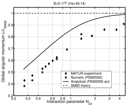
Figure 14: Global angular momentum for $B=0.17$ T, at quasi-equilibrium as a function of the interaction parameter. For low values of $N_{2d}$, the global angular momentum is reduced to about a third of its value without non-linear effects (this corresponds to a drop in the maximal azimuthal velocity to about half the SM82 value). Note that all values are normalised by the theoretical value at equilibrium derived from the SM82 model $L_{sm82}$.

Another important effect of recirculations is the ”stabilisation” of the flow. Indeed, figure 15 shows that the amplitude of the oscillations of the global angular momentum at equilibrium is strongly reduced, compared to SM82 results, which corresponds to the observation that the flow is less chaotic when significant recirculations occur. Global enstrophy (resp. energy) oscillates by around $5\%$ (resp. $10\%$) at $3$ A with PSM2000 and $30$ A with SM82. This oscillation falls below $0.1\%$ (resp. $1\%$) for $I=30$ A with PSM2000.

This is a consequence of the local damping of disturbances pointed out in section 2.3.2, which does not appear in SM82 simulations.

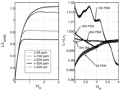
Figure 15: Evolution of the global angular momentum with time. On the left figure, curves $I=3$ A (PSM2000) and $I=30$ A (SM) nearly merge as recirculations are very weak and don’t affect the flow very much for $I=3$ A. On the right figure, quantities are normalised by their value at quasi-equilibrium, averaged over a period of $t_{H}$. The thickness of the lines give an idea of the numerical precision of the result (about $0.1\%$)

5.5.2 Transient time

The SM82 model, predicts that the system should reach the quasi-steady state in a time of the order of $t_{H}$. When important Ekman pumping occurs, the wall side layers can become thin enough to significantly increase the global dissipation. This results in shortened response time of the flow. This tendency is illustrated in Figure 16 which shows that the typical response time of the flow near quasi-equilibrium varies approximately as $N^{3/2}$ (in practise, this time is obtained by measuring the slope of the $L(t)-L(t\rightarrow\infty)$ curve near equilibrium in a log-log diagram). Using the axisymmetric assumption, the evolution equation for the angular momentum derived from the PSM2000 model can be linearised around the quasi-steady state: this provides a response time varying as $N^{2/3}Ha^{1/3}$. The reason for the difference is again that the full numerical simulation accounts for local recirculations, added to the recirculation due to global rotation by each vortex. As discussed in section 5.4.2, these additional recirculations make the wall side layer even thinner and increase the wall shear stress compared to the axisymmetric case.

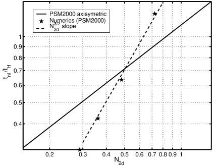
Figure 16: Transient time obtained numerically after switching on the forcing on a fluid at rest (stars) and non-linear time $t_{nl}$ derived from PSM2000 under the assumption of axisymmetry, versus total interaction parameter.

5.6 Stability of the free shear layer

The axisymmetric free shear layer located at $r=r_{e}$ is subject to a Kelvin-Helmholtz instability, which leads to the growth of cyclonic vortices along the layer. In order to get a rough estimate of the stability condition, the radial profile of azimuthal velocity is assumed linear and the layer is assumed to be of thickness $\delta=aHa^{-1/2}.$ Without viscous or electromagnetic effects, the layer is unconditionally unstable. The most unstable radial wavenumber $k$ and the related growth rate $\sigma_{c}$ are given by (see [6]):

$$k\delta=0.8$$ (21a)

$$\sigma_{c}=0.4\dfrac{U}{\delta}$$ (21b)

In the MHD problem, the magnetic field tends to stabilise the flow because of the Hartmann friction. Indeed, for small enough velocities (experimentally, theses velocities correspond to values of $I$ below $0.2$ A), the laminar parallel layer can be stable if $t_{H}^{-1}$ is bigger than the frictionless growth rate :

$$0.4\frac{U}{a}Ha^{-\frac{1}{2}}<\frac{1}{t_{H}}$$ (22)

or equivalently, using the Reynolds number $Re=Ua/\nu$:

$$\frac{Re}{Ha^{\frac{1}{2}}}<2.5$$ (23)

In other words, the piecewise linear profile chosen for the parallel layer becomes linearly unstable when the Reynolds number built on its thickness exceeds the threshold of $2.5$. At $B=0.17$ T , the typical size of the vortices appearing at the onset of instability is given by (21a) and corresponds to $2.6$ mm. [15] have performed an energetic stability study of the 2d problem, using a more realistic piecewise exponential profile. They find a stability threshold (below which any arbitrary perturbation is damped) $Re/\sqrt{Ha}=9$ and a most unstable wavelength of $2$ mm. The fact that even under slightly different assumptions, both linear and energetic stability threshold remain of comparable orders of magnitude suggests that the free shear layer is indeed destabilised by infinitesimal perturbations of typical wavelength close to the boundary layer thickness.

Finally, it is worth mentioning the effect of curvature: [16] has shown that for stably curved layers (i.e. high speed stream on the outside of the curvature) the centrifugal force tends to slightly reduce the growth rate of the Kelvin-Helmholtz unstable modes, which might increase the instability threshold, without affecting the basic mechanism.

In both numerical simulations and experiment, The destabilised state is itself unstable and the vortices merge until a small number of big structures is reached. The choice of either SM82 or PSM2000 does not affect significantly the instability found by numerical simulations. Actually, PSM2000 leads to an earlier destabilisation ($t=5$ s at $30$ A versus $t=4$ s for the SM82 model), but this is due to the fact that non-linear effects tend to reduce the characteristic response time of the flow (see section 5.5.2) so that the unstable regime is reached quicker with PSM2000. In the numerical simulations, the laminar free shear layer is only radially discretised with two or three points as explained earlier, so that the numerical profile is rather close to the piecewise linear profile studied in this section.

5.7 2d fluctuations

Radial profiles of RMS azimuthal velocity fluctuations are in good agreement with experimental measurements (see figure 17): both exhibit two extrema at $r=0.07$ m and $r=r_{e}$. The area $r=0.07$ m corresponds to the location inside the electrodes ring where the average velocity is very low but perturbed by the edge of passing vortices, which explains the important fluctuations of velocity. It also clearly appears that the relative intensity of the velocity fluctuations decreases with decreasing $N$, i.e. when secondary flows become stronger. This phenomenon is more than likely related to the smoothing effect theoretically predicted in section 2.3.2 and visible in figures 9 and 10. It should also be noticed that the velocity fluctuations can be of the order of $1$ cm/s or less. At such low velocities, the experimental results are not as precise as for higher velocities such as those in figure 13. The agreement between theory and experiment should therefore be considered to be as good as one can expect.

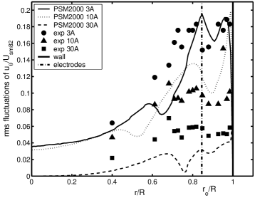
Figure 17: Radial profiles of Root Mean Square azimuthal (top) and radial (bottom) velocity fluctuations (averaged in time at quasi-steady state), for several values of the injected current.

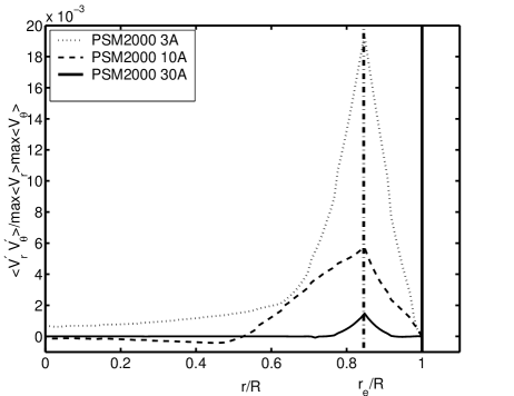
Figure 18: Radial profiles of Root Mean Square value of the correlations of velocity fluctuations (averaged on time at quasi-steady state), for several values of the injected current. Values are normalised by the maximum values reached in the time-averaged radial velocity profiles. These curves therefore give a measure of the turbulent intensity.

The damping of turbulent fluctuations by local Ekman recirculations is more visible when looking at the turbulent intensities plotted on figure 18. It shows the radial profile of $<v_{r}^{\prime}v_{\theta}^{\prime}>$, the values of which are also strongly reduced by Ekman recirculations. But what further appears, is that for higher forcing, all non-zero values of $<v_{r}^{\prime}v_{\theta}^{\prime}>$ are are confined radially around the injection electrode. For $I=20$ A and $I=30$ A, the intensity of the correlation decreases almost linearly with the distance to the electrode. In other words, apart from the fluctuations due to passage of big vortices in almost solid rotation, there is hardly any turbulent fluctuations left. Moreover, the typical width of the vortices (indicated by the width of the peak in the values of $<v_{r}^{\prime}v_{\theta}^{\prime}>$ ) strongly decreases with increasing forcing.

Four distinct mechanisms dissipate energy in the flow: turbulent dissipation, friction in the Hartmann layers, friction in the side wall and local dissipation by secondary flows. The typical ratio between turbulent dissipation and Hartmann damping is around $10^{-3}$, which confirms that turbulent dissipation is very small, as expected in 2d turbulence. The dissipation in the side layer is drastically increased by the radial transport of angular momentum due to Ekman pumping. One can get an idea about the importance of this dissipation by comparing the analytic values obtained for the angular momentum at quasi- equilibrium using SM82 (which ignores the recirculations) and PSM2000 (see figure 14). For $I=30$ A, dissipation in the side layer is of the order of the Hartmann dissipation. This analytical value is obtained under the assumption of axisymmetry and therefore ignores the local dissipation due to local recirculations. The fact that it doesn’t depart significantly from the experiment suggests that this local dissipation is rather weak.

5.8 Higher fields and turbulent Hartmann layer

For higher magnetic fields ($B=0.5$ T) and strong forcing ($I=30$ A), the ratio $Ha/N$ becomes large ($282$). This ratio also represents the Reynolds number scaled on the thickness of the Hartmann layer and it is well known that the Hartmann layer becomes turbulent when it reaches such values ($250$ according to the experimental study of [11], $380$ according to the experiments of [18] and 390 according to the numerical work of [14], see also the theoretical work by [1]). [14] also found that even when the Hartmann layer becomes turbulent, the core flow can still remain 2d. It will indeed be the case if the turnover time associated with 3d velocity fluctuations, remains smaller than the typical bidimensionalisation time. [25] have shown that if $k$ is the non-dimensional wavenumber (normalised by $1/a$) associated with one particular structure, this structure is two-dimensional if $k<<N^{-1/3}$, which can be satisfied over the whole spectrum of $k$ even for values of $Ha/N$ above the Hartmann layer stability threshold.

For such high values of $Ha/N$, the global angular momentum computed from the PSM2000 model exhibits a strong discrepancy with experimental results. The reason is that the Hartmann layer becomes turbulent. Indeed, the magnitude of non-linear effects due to Ekman recirculation is monitored by the interaction parameter $N\sim B^{2}/U$, which means that if the magnetic field is increased, the velocity has to increase as $B^{2}$ to observe non-linear effects of the same magnitude. The Hartmann layer becomes turbulent when the Reynolds number at the scale of the layer ${Re}/Ha\sim U/B\sim B/N$ exceeds a few hundred. For a fixed value of $N$ (i.e. given relative recirculation magnitude), this threshold is then lower for lower fields. In other words, for sufficiently high magnetics fields, the Hartmann layer is already turbulent when values of $U$ are reached, which are high enough to induce a significant Ekman pumping. Both SM82 and PSM2000 models rely on the assumption that the Hartmann layer is laminar and therefore cannot represent the flow above the Hartmann layer stability threshold (see figure 19).

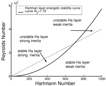
Figure 19: Hartmann layer stability and inertial effects diagram. The stability threshold is arbitrarily fixed at $Re/Ha=400$. The curve of constant amplitude inertial effects is plotted for $N=1.75$.

6 Conclusion

The comparison between the predictions derived from the PSM2000 model and the experimental results of [2] shows that the model achieves a good accuracy for all measured quantities, and this in spite of its relative simplicity. The effects of both local (at the scale of large eddies) and global (at the scale of the whole cell) recirculations are reproduced in a fairly realistic way. Moreover, the new model allows us to point out quite simply the 3d details of their mechanisms, whilst retaining the simplicity of 2d calculations. It is worth mentioning here, three of the major properties of this model. Firstly, the second-order non-linear terms yield a tendency to smooth the velocity gradients, which can ultimately erase the chaotic behaviour of the flow and damp 2d turbulence. Secondly, they induce some additional dissipation within the Parallel boundary layers in which the velocity gradients are increased. Finally, it appears that the response time of the flow is reduced. The latter effect seems to be related to the transport of any quantity by the secondary flows. Broadly speaking, the quasi-2d turbulent flow tends to be more homogeneous.

We now wish to mention two questions, which remain open. Firstly, the secondary centrifugal flows which characterise PSM2000 should certainly affect the transport of any passive scalar quantity. This might be investigated by adding an energy equation to (9) and the accuracy of the results might be checked by comparison with the temperature measurements of [2]. Second, both SM82 and PSM2000 fail to model the turbulence within the Hartmann layer when it is present. Its consequence should be to increase the layer’s thickness and the wall friction. A new MHD 2d model could be derived from the model by [1] for the turbulent Hartmann layer.

Finally, we insist that both examples of the SM82 and PSM2000 models do not only offer a method, but also prove that this method is flexible enough to make the modelling of complex 3d flows possible, as long as there is a local model for the phenomenon involved(here we combine MHD and rotation effect).

When applicable, this appears to the authors as a good alternative to fully-3d simulations which require enormous computational resources. This is all the more important as 3d CFD is sometimes only possible at the expense of rather unphysical approximations or numerical adjustments. Unlike these, PSM2000-like models are rigorously derived from the equations thanks to well controlled approximations, which ensure the reliability and clearly mark their area of validity. Thanks to these features, the refined 2d model has proven accurate enough to point out a property which had not been mentioned before to our knowledge: the non-linear smoothing by local recirculations.

This method can also be extended to any kind of quasi-2d flow, such as rotating flows. The analogy between the kind of flow described in this paper and some geophysical flows (see [20]) suggests that corrections such as those featured in PSM2000 could turn out to be efficient in modelling oceans or atmospheres. [9] has indeed recently shown that PSM2000 exhibits a very similar behaviour to the model developed by [4] for 2d turbulence.

The authors are particularly grateful to Martin Cowley for his active contribution to the presentation of the 2d models, as well as to the discussions around the meaning of these models.

References

- [1] Alboussière, T. & Lingwood, R. J. 2000 A model for the turbulent Hartmann layer. Phys. Fluids 12 (6), 1535–1543.
- [2] Alboussière, T., Uspenski, V. & Moreau, R. 1999 Quasi-2d MHD turbulent shear layers. Experimental Thermal and Fluid Science 20, 19–24.
- [3] Basdevant, C. & Sadourny, R. 1983 Parametrization of virtual scale in numerical simulation of two dimensional turbulent flows. J. Mech. Theor. Appl. Special issue, 243–269.
- [4] Benzi, R., Succi, S. & Vergassola, M. 1990 Turbulence modelling by non-hydrodynamic variables. Europhys. Lett. 13, 727–732.
- [5] Bühler, L. 1996 Instabilities in quasi two-dimensional magnetohydrodynamic flows. J. Fluid Mech. 326, 125–150.
- [6] Chandrasekkhar 1961 Hydrodynamic and Hydromagnetic Stability. Clarendon.
- [7] Davidson, P. & Pothérat, A. 2002 A note on Bodewadt-Hartmann layers. Eur. J. Mech. /B Fluids 21, 545–559.
- [8] Delannoy, Y., Pascal, B., Alboussière, T., Uspenski, V. & Moreau, R. 1999 Quasi-two-dimensional turbulence in MHD shear flows: The Matur experiment and simulations in transfer phenomena and Electroconducting flows by Alemany et Al.. Kluwer Academic Publishers.
- [9] Dellar, P. J. 2003 Quasi-two dimensional liquid metal magnetohydrodynamics and the anticipated vorticity method. J. Fluid Mech. to appear.
- [10] Greenspan, H. P. 1969 The Theory of Rotating Fluids. Cambridge University Press.
- [11] Hua, H. & Lykoudis, W. 1974 Turbulent measurements in magneto-fluid mechanics channel. Nucl. Sci. Eng. 45, 445.
- [12] Issa, R. 1986 Solution of the implicitly discretized fluid flow equations by operator-splitting. Journal of Computational Physics 62, 40–65.
- [13] Kolesnikov, Y. & Tsinober, A. 1974 Experimental investigation of two-dimensional turbulence behind a grid. Isv. Akad. Nauk. SSSR, Mech. Zhidk. Gaza. (No. 4) pp. 146–150 (in Russian).
- [14] Krasnov, D., Zienicke, E., Zikanov, O., Boeck, T. & Thess, A. 2004 Numerical study of the instability of the Hartmann layer. J. Fluid Mech. 504, 183–211.
- [15] Lieutaud, P. & Néel, M.-C. 2001 Instabilité bidimesionnelle d’une couche libre cisaillée d’origine electromagnétique. Cr. Acad. Sci, serie IIb t.329, 881–887.
- [16] Liou, W. W. 1994 Linear instability of curved free shear layers. Phys. Fluids 6 (2), 541–549.
- [17] Moreau, R. 1990 Magnetohydrodynamics. Kluwer Academic Publisher.
- [18] Moresco, P. & Alboussière, T. 2004 Experimental study of the instability of the Hartmann layer. J. Fluid Mech. 504, 167–181.
- [19] Pedlosky, J. 1987 Geophysical Fluid Dynamics. Springer Verlag.
- [20] Pothérat, A. 2000 Étude et Modèles Effectifs d’Écoulements Quasi-2d. PhD thesis, INPG, Grenoble - France.
- [21] Pothérat, A., Sommeria, J. & Moreau, R. 2000 An effective two-dimensional model for MHD flows with transverse magnetic field. J. Fluid Mech. 424, 75–100.
- [22] Pothérat, A., Sommeria, J. & Moreau, R. 2002 Effective boundary conditions for magnetohydrodynamic flows with thin Hartmann layers. Phys. Fluids 14 (1), 403–410.
- [23] Roache, P. 1997 Quantification of uncertainty in computational fluid dynamics. Ann. Rev. Fluid Mech. 29, 123–60.
- [24] Sommeria, J. 1988 Electrically driven vortices in a strong magnetic field. J. Fluid Mech. 189, 553–569.
- [25] Sommeria, J. & Moreau, R. 1982 Why, how and when MHD turbulence becomes two-dimensional. J. Fluid Mech. 118, 507–518.
- [26] Tagawa, T., Authié, G. & Moreau, R. 2002 Buoyant flow in long vertical enclosures in the presence of a strong horizontal magnetic field, Part 1: Fully-established flow. Eur. J. Mech. /B Fluids 21 (4), 383–398.
- [27] Verron, J. & Sommeria, J. 1987 Numerical simulations of a two-dimensional turbulence experiment in magnetohydrodynamics. Phys. Fluids 30, 732–739.