Dielectric constant of supercritical water in a large pressure-temperature range

Abstract

A huge amount of water at supercritical conditions exists in Earth’s interior, where its dielectric properties play a critical role in determining how it stores and transports materials. However, it is very challenging to obtain the static dielectric constant of water, $\epsilon_{0}$, in a wide pressure-temperature (P-T) range as found in deep Earth either experimentally or by first-principles simulations. Here, we introduce a neural network dipole model, which, combined with molecular dynamics, can be used to compute P-T dependent dielectric properties of water as accurately as first-principles methods but much more efficiently. We found that $\epsilon_{0}$ may vary by one order of magnitude in Earth’s upper mantle, suggesting that the solvation properties of water change dramatically at different depths. There is a subtle interplay between the molecular dipole moment and the dipolar angular correlation in governing the change of $\epsilon_{0}$. We also calculated the frequency-dependent dielectric constant of water in the microwave range, which, to the best of our knowledge, has not been calculated from first principles, and found that temperature affects the dielectric absorption more than pressure. Our results are of great use in many areas, e.g., modelling water-rock interactions in geochemistry. The computational approach introduced here can be readily applied to other molecular fluids.

I introduction

Water is arguably the most important solvent on Earth, and also largely exists inside Earth’s crust, mantle Hirschmann and Kohlstedt (2012), and even towards core Mao et al. (2017). The supercritical water at pressure (P) above 22 MPa and temperature (T) higher than 647 K is a major component of Earth’s deep fluids Liebscher (2010), storing and transporting many materials, and is also used as working fluids in various industrial areas Weingärtner and Franck (2005). The dielectric constant of supercritical water, $\epsilon_{0}$, substantially affects its solvation properties and interactions with minerals, and is a key quantity in many science and industry applications Fernandez et al. (1997); Weingärtner and Franck (2005).

For more than two decades, experimental data of the static dielectric constant of water has been limited to pressure lower than 0.5 GPa and temperature below 900 K Fernandez et al. (1995), which can be extrapolated to $\sim$1 GPa and $\sim$1300 K using various models (e.g., Fernandez et al. (1997)). However, these P-T conditions can be only found in the very shallow mantle. Experimentally, we do not know $\epsilon_{0}$ in most part of Earth’s interior, where many important aqueous reactions are happening Manning (2018). First-principles molecular dynamics (FPMD) simulations have shown reliable predictions beyond the reach of current experiments, but the computational expense is so high that the previous study reported only 5 data points Pan et al. (2013). In molecular dynamics (MD) simulations, the calculation of $\epsilon_{0}$ requires the variance of the total dipole moment of the simulation box, $\vec{M}$, so a large number of uncorrelated configurations are needed Neumann and Steinhauser (1984). For example, at ambient conditions several nanoseconds MD simulations are required to get a converged value of $\epsilon_{0}$ Gereben and Pusztai (2011). In electronic structure calculations with periodic boundary conditions, $\vec{M}$ is often calculated by the sum of molecular dipole moments using maximally localized Wannier functions (MLWFs), obtained by minimizing the spread of molecular orbitals from density functional theory (DFT) calculations Marzari et al. (2012).

In recent years, machine learning techniques emerge as an appealing tool to combine the accuracy of first-principles simulations and the efficiency of empirical force fields in atomistic simulations. In many studies, machine learning models were trained using data from first-principles calculations to learn potential energy surfaces, which can be further used in MD or Monte Carlo simulations (e.g., refs Behler and Parrinello (2007); Bartók et al. (2010); Rupp et al. (2012); Smith et al. (2017); Zhang et al. (2018)). Some electronic properties may be also obtained using machine learning models, e.g., the dielectric constant of a variety of crystals Umeda et al. (2019), but how the dielectric constant varies with environmental factors like P or T is not known.

Here, we constructed a neural network dipole (NND) model using data from FPMD simulations to calculate the molecular dipole moment of supercritical water. In combination with MD trajectories obtained by the machine learning force field, we calculated the dielectric constant of water from 1 to 15 GPa and 800 to 1400 K, where $\epsilon_{0}$ changes by one order of magnitude. We also calculated the frequency-dependent dielectric constant of water, and found that temperature affects the dielectric absorption peak more than pressure. The accurate and efficient method of calculating dielectric constant of water in a large P-T range makes it possible to model aqueous solutions and water-rock interactions in a large part of Earth’s interior. Our results have great implications on the solvation properties of aqueous geofluids in deep Earth.

II Implementation details

In MD simulations with periodic boundary conditions, the dielectric constant of an isotropic and homogeneous fluid can be calculated by Neumann and Steinhauser (1984); Sharma et al. (2007):

$$\begin{split}\epsilon_{0}=\epsilon_{\infty}+\frac{4\pi}{3k_{B}TV}\left(\left\langle\vec{M}^{2}\right\rangle-\langle\vec{M}\rangle^{2}\right),\end{split}$$ (1)

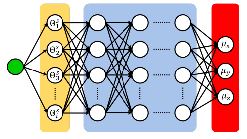
Figure 1: Structure of the neural network used to output the molecular dipole moment. The green circle refers to the solvation shell structure as the initial data. The yellow, blue, and read blocks represent the input, hidden, and output layers, respectively. The molecular dipole moment, $\vec{\mu}$, is expressed using local coordinates, $(\mu_{x},\mu_{y},\mu_{z})$.

where $\epsilon_{\infty}$ is the electronic dielectric constant, $k_{B}$ is the Boltzmann constant, $T$ is the temperature, $V$ is the volume of the simulation box. $\epsilon_{\infty}$ can be calculated by density functional perturbation theory Baroni et al. (2001), whose fluctuation is much smaller than that of $\epsilon_{0}$, so tens of MD configurations are enough to get converged results Pan et al. (2014). The calculation of the variance of $\vec{M}$ requires a large number of uncorrelated MD configurations and the simulation box cannot be too small, so if we directly build a machine learning model to obtain $\vec{M}$ Grisafi et al. (2018), the training set has to sample the huge configuration space well, which can be very expensive. Instead, here we constructed the machine learning model to get the molecular dipole moment of water in fluids. In DFT calculations, there are 64$\sim$128 water molecules in one simulation box, so we have 64$\sim$128 independent water dipoles from one MD configuration, which makes it easier to have a large training set. The dipole moment of water molecules strongly depends on their local chemical environment Pan et al. (2013), so we chose the local solvation structure as input to an end-to-end neural network model as shown in Fig. 1. We built a local Cartesian coordinate for each water molecule based on its molecular geometry. The origin is located at the O atom of the center water molecule. The $x$ axis is along the bisector of $\angle$HOH, and the $z$ axis is perpendicular to the plane formed by one O and two H atoms. In this way, the rotational and translational symmetries are preserved. For the center water molecule, the input is the coordinates of its neighboring atoms including its two H atoms $\vec{\Theta}=\{\Theta^{O}_{1},\Theta^{O}_{2},...,\Theta^{O}_{i},...;\Theta^{H}_{1},\Theta^{H}_{2},...,\Theta^{H}_{i},...\}$ within a cutoff radius R_c:

$$\Theta^{s}_{i}=\{\frac{x_{i}}{r_{i}^{3}},\frac{y_{i}}{r_{i}^{3}},\frac{z_{i}}{r_{i}^{3}}\},r_{i}\leq R_{c},$$ (2)

where $(x_{i},y_{i},z_{i})$ is the local Cartesian coordinate of the $i$th neighboring atom, $s$ labels the species as either O or H, and $r_{i}=\sqrt{x_{i}^{2}+y_{i}^{2}+z_{i}^{2}}$. We sorted the atoms by distance from near to far in the input to preserve the permutational symmetry. We fixed the cutoff radius at 0.6 nm, and $\vec{\Theta}$ has the coordinates of 32 water molecules. In our study, the water density varies considerably, so if the number of water molecules within this radius was smaller than 32, we appended (0,0,0) to the tail of $\vec{\Theta}$ to keep the size of $\vec{\Theta}$ constant.

In the neural network model, we used four hidden layers, sequentially consisting of 300, 200, 100, and 30 nodes, to connect the input and output layers. We chose the hyperbolic tangent function Abadi et al. (2015) as the activation function for all hidden layers. The loss function is defined as,

$$\begin{split}L=\frac{1}{n}\sum_{j=1}^{n}[(\vec{\mu}^{p}_{j}-\vec{\mu}^{t}_{j})^{2}+(\norm{\vec{\mu}^{p}_{j}}-\norm{\vec{\mu}^{t}_{j}})^{2}]\end{split}$$ (3)

where $\vec{\mu}^{p}_{j}$ and $\vec{\mu}^{t}_{j}$ are the predicted and inputted dipole moments of the $i$th water molecule, respectively, and $n$ is the batch size. We used the Adam optimization algorithm Kingma and Ba (2014) to minimize the loss function and the learning rate is 1.0 $\times 10^{-4}$. To avoid overfitting, we added a L2 regularization Ng (2004) to each hidden layer.

Our training set consists of 2138880 water dipoles obtained from over 100 ps FPMD simulations at ambient and supercritical conditions up to 11 GPa and 2000 K. Although our current study is focused on supercritical water, we found that the data at ambient conditions could improve the accuracy of the trained NND model.

To calculate the dipole moment of water molecules, we used the PBE xc functional Perdew et al. (1996), which may not be sufficient enough to describe hydrogen bonds in water at ambient conditions Zhang et al. (2011), but our previous studies indicated that it performs better at high P and high T than at ambient conditions Pan and Galli (2016), particularly for dielectric properties Pan et al. (2013, 2014).

III results and discussion

We compared the distributions of dipole magnitude of water molecules obtained by the NND model and DFT in the test set (see Fig. S1), where the mean absolute error (MAE) is 0.14 D. Interesting, we also tested our NND model at 30 GPa and 2000 K, which was not included in the training set, and the MAE is 0.038 D. The water ionization happens very frequently at this condition, so we use one O atom and two nearest H atoms to form a water ‘molecule’ to calculate the molecular dipole. The excellent performance at 30 GPa and 2000 K suggests that our NND model can not only cover the P-T range of the training set, but may also be extrapolated outside this range.

In Fig. S2 we plotted the distributions of the angle between the dipole moment vectors calculated by the NND model and DFT, and the MAE is 3.86^∘ for individual dipole moments. It is interesting to see that the error of $\vec{M}$ is slightly smaller than that of individual dipoles, which may be due to the error cancellation in the vector summation.

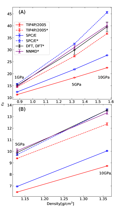
Figure 2: Static dielectric constant of water as a function of density. Two temperatures are compared: (A) 1000 K and (B) 2000 K. Results are obtained from the MD trajectories using the DFT, neural network (NNMD), and empirical force fields (SPC/E, TIP4P/2005). The asterisk (*) denotes that the trajectory is from the corresponding force field, while molecular dipoles are calculated using the neural network dipole model. The DFT and DFT* results are indistinguishable. Error bars are obtained by the blocking method Flyvbjerg and Petersen (1989).

After validating water dipole moments obtained by our NND model, we applied them to calculate $\epsilon_{0}$ at various P-T conditions as shown in Fig. 2. At each P-T condition, we used half of the MD trajectory to train the NND model and the remaining half to assess results. Overall, the relative error is smaller than 0.6% in test sets, which is much smaller than the standard deviations obtained from our MD simulations, indicating that our NND model is nearly as accurate as first principles calculations (see Table SI).

After building an excellent model to calculate the molecular dipole moment of water, we may conduct first-principles MD simulations to generate trajectories at various P-T conditions and then use the NND model to calculate the fluctuation of $\vec{M}$ to get the dielectric constant of water. Using this method, we avoid the step of calculating MLWFs. However, the FPMD simulation is also very expensive, which limits its application to many P-T conditions. In many previous studies on high P-T water, the force fields SPC/E Berendsen et al. (1987) and TIP4P/2005 Abascal and Vega (2005) were widely used. Although they were mainly designed to simulate ambient water, they seem to work well for some properties at high P and T, e.g., the equation of state Zhang and Duan (2005). As for dielectric properties, the main limitation of these two models is their rigidity. The molecular dipole moment of SPC/E is fixed at 2.34 D, while that of TIP4P/2005 is 2.31 D. In fact, both P and T may affect the molecular dipole moment of water considerably. Our previous study shows that at $\sim$1 GPa and 1000 K, the dielectric constant of water calculated by the SPC/E model is close to the result obtained from FPMD simulations and also the extrapolated experimental value Pan et al. (2013); however, the difference between the SPC/E result and that from FPMD simulations becomes larger with increasing pressure. We found that at $\sim$1 GPa and 1000 K, the average dipole moment of water molecules, $\mu$, calculated by DFT is close to 2.34 D, but $\mu$ increases with increasing pressure and decreases with increasing temperature, which cannot be captured by rigid water models.

Since our NND model gives excellent dipole distributions under various P-T conditions, we applied this model to calculate molecular dipole moments for the trajectories obtained from the SPC/E and TIP4P/2005 simulations, as shown in Fig. 2. The dielectric constants calculated by our NND model are generally larger than those directly from the two water models, and become closer to the DFT values, indicating that the polarization of water molecules with pressure and temperature affects the dielectric constant of water.

It is interesting to see that the dielectric constants calculated by the SPC/E model are closer to the DFT values than those by the TIP4P/2005 model, whereas at 1000 K using the NND model the TIP4P/2005 trajectories give better results than the SPC/E ones. The dielectric constant of water depends on two factors: (1) molecular dipole moment and (2) hydrogen bond network characterized by the Kirkwood g-factor Kirkwood (1939):

$$G_{k}=\frac{\langle\vec{M}^{2}\rangle}{N\mu^{2}},$$ (4)

where $N$ is the number of molecules in the simulation box. Vega et al. argued that for high pressure ice phases at 243 K, TIP4P/2005 may provide decent $G_{k}$, so after scaling the molecular dipole moment, it gives correct dielectric constants Aragones et al. (2011), which is qualitatively consistent with our finding at 1000 K. However, when increasing T to 2000 K, the SPC/E trajectories perform better again than TIP4P/2005, indicating that the SPC/E model may give more accurate $G_{k}$ than TIP4P/2005 at very high temperature.

The variation of molecular geometry of water can not be well reproduced by rigid force fields. Here, we also generated MD trajectories using the neural network force field, which was recently developed for high P-T water and ice in the molecular, ionic, and superionic phases up to 70 GPa and 3000 K using the DFT energy potential Zhuang et al. (2020). We calculated $\epsilon_{0}$ using the obtained water trajectories, as shown in Fig. 2. The difference between the NND and DFT values is smaller than 1.7% , which is within error bars in FPMD simulations and overall better than the results obtained from the SPC/E and TIP4P/2005 trajectories.

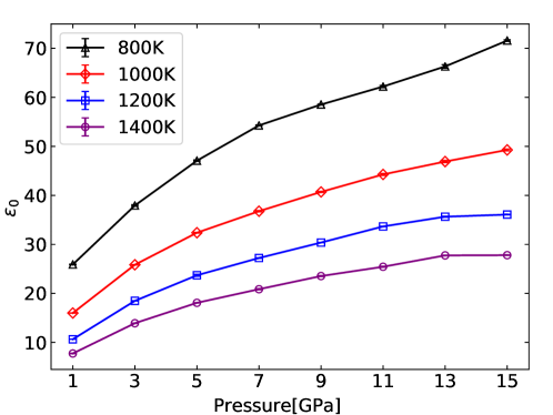
Figure 3: Static dielectric constant of supercritical water at high P-T conditions. Molecular dipoles are calculated using the neural network dipole model and trajectories are from simulations with the neural network force field. Error bars are within symbols. The equation of state of water is from Ref. Zhang and Duan (2005).

Using the NND model and the neural network force field, we calculated the dielectric constant of supercritical water from 1 to 15 GPa and 800 to 1400 K, corresponding to the P-T conditions found in Earth’s upper mantle. $\epsilon_{0}$ increases with increasing P and decreases with increasing T, and varies from $\sim$7 up to 72 in Fig. 3. Generally, the increase of $\epsilon_{0}$ becomes smaller with increasing P along an isotherm. Since $\epsilon_{0}$ determines the solvation properties of water, the large variation of $\epsilon_{0}$ substantially influences how water stores and transports materials with great implications on water-rock interactions in Earth’s interior.

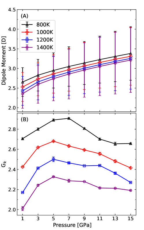
Figure 4: Molecular dipole moments and the Kirkwood g-factor, $G_{k}$, of water at high P-T conditions. (A) The average molecular dipole moment and standard derivation as a function of pressure. (B) $G_{k}$ as a function of pressure.

Fig. 4 shows $\mu$ and $G_{k}$ as a function of pressure. With increasing P along an isotherm, $\mu$ increases monotonically, whereas $G_{k}$ increases and then decreases; its peak appears at 5$\sim$7 GPa. $G_{k}$ accounts for the dipolar angular correlation. With increasing P from 1 to 5 GPa, the angular correlation among dipoles is enhanced because the molecular interaction becomes stronger. With increasing P further, however, the hydrogen bonding becomes weaker due to the increased coordination number Schwegler et al. (2000), so the angular correlation is not as strong as at low P. There is a subtle interplay between $\mu$ and $G_{k}$ in governing the change of $\epsilon_{0}$. The increase of $\epsilon_{0}$ at low P is driven by the increase of $\mu$, $G_{k}$, and water density, while at high P it is because the increase of $\mu$ and density exceeds the decrease of $G_{k}$; as a result, the increase of $\epsilon_{0}$ at high P is generally smaller than that at low P.

The dielectric constant is a function of the electric field frequency, $\epsilon(\omega)$, which can be calculated by the Fourier-Laplace transform of the derivative of the normalized autocorrelation function of $\vec{M}$, $\Phi(t)=\frac{<\vec{M}(0)\cdot\vec{M}(t)>}{<\vec{M}^{2}>}$ Neumann and Steinhauser (1984):

$$\frac{\epsilon(\omega)-\epsilon_{\infty}}{\epsilon_{0}-\epsilon_{\infty}} =\int_{0}^{\infty}(-\frac{d\Phi(t)}{dt})e^{-i\omega t}dt.$$ (5)

It is difficult to get converged $\epsilon(\omega)$ in the microwave range from FPMD simulations. Using the NND model and the neural network force field, we found that the rapid decay part of $\Phi(t)$ can be well fitted to an exponential function $Ae^{-\frac{t}{\tau_{D}}}$, where $\tau_{D}$ approximates the Debye relaxation time van der Spoel et al. (1998), with fitting errors smaller than 2.3%. In our calculations, $\Phi(t)$ contains the raw data until it decreases to 0.2, the tail from the exponential function after $\Phi(t)$ is smaller than 0.1, and the linear interpolation between the raw and fitted data when $\Phi(t)$ is between 0.2 and 0.1 to make a smooth connection. Fig. 5 shows the real and imaginary parts of the frequency-dependent dielectric constant of supercritical water in the microwave range. The large peaks in Fig. 5(B) correspond to the main dielectric absorption peaks, which are centered between about 600 GHz and 10 THz, much larger than that at ambient conditions, $\sim$ 20 GHz. The main absorption peak is upshifted with increasing temperature, but downshifted with increasing pressure. The rise of temperature from 1000 to 2000 K affects the peak position more than the increase of pressure from 1 to 10 GPa. The dielectric absorption of water may be attributed to single molecule or large collection motions, which is still under debate Elton (2017). For supercritical water studied here, it seems temperature has more obvious effects on the Debye relaxation time than pressure.

Note that very recently Zhang et al. introduced a neural network model to obtain the position of MLWF centers Zhang et al. (2020), which can be also used to calculate molecular dipole moments, but this method may be not as efficient as the NND model introduced here, considering that we need to calculate four MLWF center positions in one water molecule.

IV Conclusion

In summary, we built a neural network dipole model, which combines the accuracy of first principles calculations and the efficiency of empirical models, to compute the dielectric constant of supercritical water, $\epsilon_{0}$, from 1 to 15 GPa and 800 to 1400 K. We found that $\epsilon_{0}$ can vary by one order of magnitude in Earth’s upper mantle, suggesting that solvation properties of water may change dramatically at different depths, so water, as an important mass transfer medium, may dissolve some materials, e.g., carbon Hazen and Schiffries (2013), and transport and release them in some shallow areas, which connects material reservoirs in Earth’s surface and interior. A subtle interplay between the molecular dipole moment and the dipolar angular correlation governs the increase of $\epsilon_{0}$ with pressure. We also calculated the dielectric constant as a function of the electric field frequency, and found that temperature affects the dielectric absorption peak more than pressure in the P-T range studied here. The accuracy of our method solely depends on the quality of the training data, which can be further improved by using high level theories, e.g., hybrid exchange-correlation functionals in DFT. Although we studied only water here, our method can be readily applied to other molecular fluids.

The dielectric constant of water as a function of P and T plays a key role in the Deep Earth Water (DEW) model developed recently, which can calculate thermodynamic properties of many aqueous species and study water-rock interactions at elevated P-T conditions Huang and Sverjensky (2019). Using the method introduced here, we are able to build a high quality database for $\epsilon_{0}$ in a large P-T range as found in deep Earth. The obtained data has great implications on how water stores and transports materials in Earth’s interior.

V Acknowledgments

We thank Giulia Galli and Viktor Rozsa for their helpful discussions, and Lin Zhuang and Xin-Zheng Li for helping the simulations with the neural network force field. D.P. acknowledges support from the Croucher Foundation through the Croucher Innovation Award, Hong Kong Research Grants Council (Projects ECS-26305017 and GRF-16307618), National Natural Science Foundation of China (Project 11774072), and the Alfred P. Sloan Foundation through the Deep Carbon Observatory. Part of this work was carried out using computational resources from the National Supercomputer Center in Guangzhou, China.

VI Author contributions

D.P. designed research; R.H., Y.Q, and D.P. performed research; R.H., Y.Q, and D.P. analyzed data; and R.H. and D.P. wrote the paper.

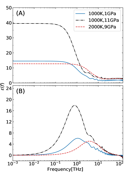
Figure 5: Frequency-dependent dielectric constant of water, $\epsilon(f)$, at high P-T conditions. The real and imaginary parts of $\epsilon(f)$ in the microwave range are shown in (A) and (B), respectively ($\omega=2\pi f$).

References

- Hirschmann and Kohlstedt (2012) Marc Hirschmann and David Kohlstedt, “Water in Earth’s mantle,” Phys Today 65, 40 (2012).
- Mao et al. (2017) Ho-Kwang Mao, Qingyang Hu, Liuxiang Yang, Jin Liu, Duck Young Kim, Yue Meng, Li Zhang, Vitali B Prakapenka, Wenge Yang, and Wendy L Mao, “When water meets iron at Earth’s core–mantle boundary,” Natl Sci Rev 4, 870–878 (2017).
- Liebscher (2010) Axel Liebscher, “Aqueous fluids at elevated pressure and temperature,” Geofluids 10, 3–19 (2010).
- Weingärtner and Franck (2005) Hermann Weingärtner and Ernst Ulrich Franck, “Supercritical water as a solvent,” Angew Chem Int Ed Engl 44, 2672–2692 (2005).
- Fernandez et al. (1997) DP Fernandez, ARH Goodwin, Eric W Lemmon, JMH Levelt Sengers, and RC Williams, “A formulation for the static permittivity of water and steam at temperatures from 238 k to 873 k at pressures up to 1200 mpa, including derivatives and Debye–Hückel coefficients,” J Phys Chem Ref Data 26, 1125–1166 (1997).
- Fernandez et al. (1995) Diego P Fernandez, Y Mulev, ARH Goodwin, and JMH Levelt Sengers, “A database for the static dielectric constant of water and steam,” J Phys Chem Ref Data 24, 33–70 (1995).
- Manning (2018) Craig E. Manning, “Fluids of the lower crust: Deep is different,” Annu Rev Earth Planet Sci 46, 67–97 (2018).
- Pan et al. (2013) D. Pan, L. Spanu, B. Harrison, D. A. Sverjensky, and G. Galli, “Dielectric properties of water under extreme conditions and transport of carbonates in the deep Earth,” Proc Natl Acad Sci USA 110, 6646–6650 (2013).
- Neumann and Steinhauser (1984) M. Neumann and O. Steinhauser, “Computer simulation and the dielectric constant of polarizable polar systems,” Chem Phys Lett 106, 563–569 (1984).
- Gereben and Pusztai (2011) Orsolya Gereben and László Pusztai, “On the accurate calculation of the dielectric constant from molecular dynamics simulations: The case of SPC/E and SWM4-DP water,” Chem Phys Lett 507, 80–83 (2011).
- Marzari et al. (2012) Nicola Marzari, Arash A. Mostofi, Jonathan R. Yates, Ivo Souza, and David Vanderbilt, “Maximally localized wannier functions: Theory and applications,” Rev Mod Phys 84, 1419–1475 (2012).
- Behler and Parrinello (2007) Jörg Behler and Michele Parrinello, “Generalized neural-network representation of high-dimensional potential-energy surfaces,” Phys Rev Lett 98, 146401 (2007).
- Bartók et al. (2010) Albert P. Bartók, Mike C. Payne, Risi Kondor, and Gábor Csányi, “Gaussian approximation potentials: The accuracy of quantum mechanics, without the electrons,” Phys Rev Lett 104, 136403 (2010).
- Rupp et al. (2012) Matthias Rupp, Alexandre Tkatchenko, Klaus-Robert Müller, and O. Anatole von Lilienfeld, “Fast and accurate modeling of molecular atomization energies with machine learning,” Phys Rev Lett 108, 058301 (2012).
- Smith et al. (2017) J. S. Smith, O. Isayev, and A. E. Roitberg, “ANI-1: an extensible neural network potential with DFT accuracy at force field computational cost,” Chem Sci 8, 3192–3203 (2017).
- Zhang et al. (2018) Linfeng Zhang, Jiequn Han, Han Wang, Roberto Car, and Weinan E, “Deep potential molecular dynamics: A scalable model with the accuracy of quantum mechanics,” Phys Rev Lett 120, 143001 (2018).
- Umeda et al. (2019) Yuji Umeda, Hiroyuki Hayashi, Hiroki Moriwake, and Isao Tanaka, “Prediction of dielectric constants using a combination of first principles calculations and machine learning,” Jpn J Appl Phys 58, SLLC01 (2019).
- Sharma et al. (2007) Manu Sharma, Raffaele Resta, and Roberto Car, “Dipolar correlations and the dielectric permittivity of water,” Phys Rev Lett 98, 247401 (2007).
- Baroni et al. (2001) Stefano Baroni, Stefano De Gironcoli, Andrea Dal Corso, and Paolo Giannozzi, “Phonons and related crystal properties from density-functional perturbation theory,” Rev Mod Phys 73, 515 (2001).
- Pan et al. (2014) Ding Pan, Quan Wan, and Giulia Galli, “The refractive index and electronic gap of water and ice increase with increasing pressure,” Nat Commun 5, 3919 (2014).
- Grisafi et al. (2018) Andrea Grisafi, David M. Wilkins, Gábor Csányi, and Michele Ceriotti, “Symmetry-adapted machine learning for tensorial properties of atomistic systems,” Phys Rev Lett 120, 036002 (2018).
- Abadi et al. (2015) Martín Abadi, Ashish Agarwal, Paul Barham, Eugene Brevdo, Zhifeng Chen, Craig Citro, Greg S. Corrado, Andy Davis, Jeffrey Dean, Matthieu Devin, Sanjay Ghemawat, Ian Goodfellow, Andrew Harp, Geoffrey Irving, Michael Isard, Yangqing Jia, Rafal Jozefowicz, Lukasz Kaiser, Manjunath Kudlur, Josh Levenberg, Dandelion Mané, Rajat Monga, Sherry Moore, Derek Murray, Chris Olah, Mike Schuster, Jonathon Shlens, Benoit Steiner, Ilya Sutskever, Kunal Talwar, Paul Tucker, Vincent Vanhoucke, Vijay Vasudevan, Fernanda Viégas, Oriol Vinyals, Pete Warden, Martin Wattenberg, Martin Wicke, Yuan Yu, and Xiaoqiang Zheng, “TensorFlow: Large-scale machine learning on heterogeneous systems,” (2015), software available from tensorflow.org.
- Kingma and Ba (2014) Diederik P. Kingma and Jimmy Ba, “Adam: A method for stochastic optimization,” arXiv:1412.6980 (2014).
- Ng (2004) Andrew Y. Ng, “Feature selection, L1 vs. L2 regularization, and rotational invariance,” in Proceedings of the Twenty-First International Conference on Machine Learning, ICML ’04 (Association for Computing Machinery, New York, NY, USA, 2004) p. 78.
- Perdew et al. (1996) John P. Perdew, Kieron Burke, and Matthias Ernzerhof, “Generalized gradient approximation made simple,” Phys Rev Lett 77, 3865–3868 (1996).
- Zhang et al. (2011) Cui Zhang, Davide Donadio, Francois Gygi, and Giulia Galli, “First principles simulations of the infrared spectrum of liquid water using hybrid density functionals,” J Chem Theory Comput 7, 1443–1449 (2011).
- Pan and Galli (2016) D. Pan and G. Galli, “The fate of carbon dioxide in water-rich fluids under extreme conditions,” Sci Adv 2, e1601278 (2016).
- Berendsen et al. (1987) H. J. C. Berendsen, J. R. Grigera, and T. P. Straatsma, “The missing term in effective pair potentials,” J Phys Chem 91, 6269–6271 (1987).
- Abascal and Vega (2005) J. L. F. Abascal and C. Vega, “A general purpose model for the condensed phases of water: TIP4P/2005,” J Chem Phys 123, 234505 (2005).
- Zhang and Duan (2005) Zhigang Zhang and Zhenhao Duan, “Prediction of the PVT properties of water over wide range of temperatures and pressures from molecular dynamics simulation,” Phys Earth Planet Inter 149, 335 – 354 (2005).
- Kirkwood (1939) John G Kirkwood, “The dielectric polarization of polar liquids,” J Chem Phys 7, 911–919 (1939).
- Aragones et al. (2011) JL Aragones, LG MacDowell, and C Vega, “Dielectric constant of ices and water: a lesson about water interactions,” J Phys Chem A 115, 5745–5758 (2011).
- Zhuang et al. (2020) Lin Zhuang, Qijun Ye, Ding Pan, and Xin-Zheng Li, “Discriminating high-pressure water phases using rare-event determined ionic dynamical properties,” Chinese Phys Lett 37, 043101 (2020).
- Schwegler et al. (2000) Eric Schwegler, Giulia Galli, and François Gygi, “Water under pressure,” Physical Review Letters 84, 2429 (2000).
- van der Spoel et al. (1998) David van der Spoel, Paul J. van Maaren, and Herman J. C. Berendsen, “A systematic study of water models for molecular simulation: Derivation of water models optimized for use with a reaction field,” J Chem Phys 108, 10220–10230 (1998).
- Elton (2017) Daniel C. Elton, “The origin of the Debye relaxation in liquid water and fitting the high frequency excess response,” Phys Chem Chem Phys 19, 18739–18749 (2017).
- Zhang et al. (2020) Linfeng Zhang, Mohan Chen, Xifan Wu, Han Wang, Weinan E, and Roberto Car, “Deep neural network for the dielectric response of insulators,” Physical Review B 102 (2020), 10.1103/physrevb.102.041121.
- Hazen and Schiffries (2013) Robert M Hazen and Craig M Schiffries, “Why deep carbon?” Rev Mineral Geochem 75, 1–6 (2013).
- Huang and Sverjensky (2019) Fang Huang and Dimitri A Sverjensky, “Extended deep earth water model for predicting major element mantle metasomatism,” Geochimica et Cosmochimica Acta 254, 192–230 (2019).
- Flyvbjerg and Petersen (1989) Henrik Flyvbjerg and Henrik Gordon Petersen, “Error estimates on averages of correlated data,” J Chem Phys 91, 461–466 (1989).