Ancilla-assisted frequency estimation under phase covariant noises with Greenberger-Horne-Zeilinger states

Abstract

It has been demonstrated that the optimal sensitivity achievable with Greenberger-Horne-Zeilinger states is the same as that with uncorrelated probes in the frequency estimation in the presence of uncorrelated Markovian dephasing [S. F. Huelga, et al., Phys. Rev. Lett. 79, 3865 (1997)]. Here, we extend this issue by examining the optimal frequency sensitivities achievable by the use of ancilla-assisted strategy, which has been proposed recently for robust phase estimation. We present the ultimate frequency sensitivities bounded by the quantum Fisher information for a general case in the presence of Markovian covariant phase noises, and the optimal measurement observables that can saturate the theoretical sensitivity bounds. We also demonstrate the effectiveness of the ancilla-assisted strategy for preserving frequency sensitivities suffering from specific physically ground noises.

1 Introduction

Quantum enhanced metrology plays an important role in super-precision measurement applications, such as atomic frequency standards Wineland1994PRA ; Bollinger1996PRA ; Leibfried2004SCI , quantum magnetometers Taylor2008NP ; Goldstein2011PRL , gravitational wave detection Collaboration2011NP ; Aasi2013NP ; Barsotti2018RP , quantum gyroscopes Halkyard2010PRA ; Helm2015PRL ; Stevenson2015PRL etc. It has been attracted intense attention owing to its potential ability to improve measurement precision by a factor of $\sqrt{N}$ improvement over the standard quantum limit $1/\sqrt{N}$, where $N$ is the number of samples, such as atoms or photons Giovannetti2006PRL ; Giovannetti2011 . This is well-known Heisenberg limit $1/N$ and attainable by means of Greenberger-Horne-Zeilinger (GHZ) states Giovannetti2006PRL ; Giovannetti2011 . However, these exotic states are of extremely delicate and fragile. They may be easily destroyed by inevitabl e noises in realistic experiments and lose its capacity in sensitivity enhancement Froewis2011PRL ; Ma2011PRA ; Chaves2012PRA ; Zhong2013PRA . In 1997, Huelga et al. first found that, in frequency estimation, the sensitivity achievable with GHZ states is the same as that with uncorrelated probes in the presence of the uncorrelated Markovian dephasing noise Huelga1997PRL . Recently, more generalized results indicated that any small amount of realistic noise restricts the advantage of quantum strategies to an improvement by a constant factor Escher2011NP ; Demkowicz-Dobrzanski2012nc .

Under pressure by these no-go results, various strategies have been put forward in the literature to mitigate the detrimental effects of noise on sensitivities, including quantum error correction Duer2014PRL ; Arrad2014PRL ; Kessler2014PRL ; Lu2015NC ; Herrera-Marti2015PRL ; Unden2016PRL ; Layden2019PRL ; Sekatski2017quantummetrology , dynamical decoupling Sekatski2016NJP ; Tan2013PRA , time-continuous monitoring Gammelmark2013PRA ; Gammelmark2014PRL ; Catana2014PRA ; Kiilerich2014PRA ; Kiilerich2016PRA ; Plenio2016PRA ; Cortez2017PRA ; Chase2009PRA ; Stockton2004PRA ; Geremia2003PRL ; Albarelli2017NJP etc. Among these, a novel ancilla-assisted strategy has been proposed recently by entangling the probes with the ancillary qubits which are free from phase encoding and decoherence Demkowicz-Dobrzafmmodecutenlseniski2014PRL ; Huang2016PRA ; Huang2018PRA . This strategy has been identified as an effective way of preserving sensitivities in phase estimation under some noisy channels and also experimentally demonstrated Sbroscia2018PRA ; Wang2018PRA . These analyses were carried out only for the case of phase estimation, but there is no evidence on the effectiveness of the ancilla-assisted strategy for frequency estimation. More recently, some evidences have shown that the ultimate lower sensitivity bounds in noisy frequency estimation with and without ancillary qubits are the same in the asymptotic limit of $N\rightarrow\infty$ Smirne2016PRL . It is still ambiguous whether the ancilla-assisted strategy is useful or not for noisy frequency estimation with finite number of probes.

In this work, we address this issue by examining the sensitivities achievable with generalized GHZ states in frequency estimation suffering from a general class of Markovian noises, of which the processes commute with the unitary evolution governed by the system Hamiltonian, which is referred as phase covariant noises Smirne2016PRL . To identify the effectiveness of the ancilla-assisted strategy in noisy frequency estimation, we preform our study based on quantum estimation theory Helstrom1976Book ; Holevo1982Book ; Braunstein1994PRL and exactly obtain the ultimate frequency sensitivities achievable in aforementioned noisy scenarios. Meanwhile, the measurement observables that approach the sensitivity bounds to frequency are also presented. We then specialize these results to the most popular three kinds of decoherence models, such as phase damping channel (DPC), and amplitude-damping channel (PDC) and depolarizing channel (DPC), and obtain the optimal frequency sensitivities in these three cases. We also compare the performances of two strategies equipped with and without ancillary qubits.

This paper is organized as follows. In Sec. II, we briefly introduce background information about quantum frequency estimation in the presence of phase covariant noises. We then derive the frequency sensitivities attainable with generalized GHZ states for both ancilla-free and ancilla-assisted strategies and show the optimal measurement observables to access these sensitivities. In Sec. III, we specialize into three conventional quantum channels, such as ADC, PDC, and DPC. Finally, our conclusions are made in Sec. IV. In appendix, some derivations are presented in detail.

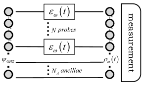
Figure 1: (Color online) Schematic of noisy frequency estimation with generalized GHZ states.

2 Noisy quantum frequency estimation

2.1 Frequency estimation in the presence of phase covariant noises

In general, an unknown parameter $\omega$ (specifically the detuning between the frequency of the atomic transition and the frequency of the driving field) to be estimated is unitarily encoded on $N$ probes, i.e., two-level atoms or qubits, of which the initial state is denoted by $\rho\left(0\right)$, over the interrogation time $t$ Huelga1997PRL . After the encoding process, the value of $\omega$ is inferred from the outcomes of the measurement on the final state of the system $\rho_{\omega}\left(t\right)$. To accurately infer its value, these processes are required to be repeated many times denoted as $\upsilon$, and the total experiment time is taken as $T=\upsilon t$. Hence, the two quantities $N$ and $T$ suggest the total resource consumed in a frequency estimation task. According to quantum estimation theory, the theoretical sensitivity limit to an unbiased frequency estimator $\hat{\omega}$ is bounded by the inverse of quantum Fisher information (QFI) Helstrom1976Book ; Holevo1982Book ; Braunstein1994PRL

$$\Delta^{2}\hat{\omega}T\geq\frac{t}{F\left[\rho_{\omega}\left(t\right)\right]}.$$ (1)

It means that the larger value of the QFI is the higher sensitivity could acquire. The above bound could be attained by the use of the maximal likelihood estimator for sufficiently large number of repetitions of the experiment Helstrom1976Book ; Holevo1982Book ; Braunstein1994PRL .

In realistic settings, it is inevitable that noises will be introduced to the encoding process and negatively affect the estimation sensitivity that one can obtain. Suppose that the evolution of each probe is independent identical. Since any quantum process can be described as a completely positive and trace-preserving (CPT) map $\mathcal{E}$, thus a noisy encoding process can be expressed by

$$\rho_{\omega}\left(t\right)=\mathcal{E}_{\omega}\left(t\right)^{\otimes N}\rho\left(0\right),$$ (2)

where $\rho\left(0\right)$ denotes the initial state of the system and $\mathcal{E}_{\omega}\left(t\right)$ represents the dynamical map on a single qubit. Here, we concentrate on a general class of phase covariant maps requiring that a CPT map $\mathcal{E}_{\omega}\left(t\right)$ can be divided into two parts: unitary encoding $\mathcal{U}_{\omega}\left(t\right)$ and frequency-independent dissipative part $\Gamma\left(t\right)$ and they commute with each other, i.e.,

$$\mathcal{E}_{\omega}\left(t\right)=\Gamma\left(t\right)\circ\mathcal{U}_{\omega}\left(t\right)=\mathcal{U}_{\omega}\circ\Gamma\left(t\right).$$ (3)

This means that one can freely exchange the order of the operations between the encoding and the dissipation.

To intuitively describe the noisy encoding processes, we take a geometric point of view in the way a single qubit state is denoted by a real vector $\bm{r}$ in the space of Pauli matrices, which is known as the so-called Bloch vector. Under the Bloch representation, the phase covariant map $\mathcal{E}_{\omega}\left(t\right)$ can be equivalently represented by an affine map Smirne2016PRL ; Zhong2013PRA

$$\mathcal{E}_{\omega}\left(t\right):\bm{r}\mapsto A\bm{r}+\bm{c},$$ (4)

where the transformation matrix $A$ is a $3\times 3$ real matrix depicted by

$$A=\left(\begin{array}[]{ccc}\eta_{\perp}\left(t\right)\cos\theta\left(t\right)&-\eta_{\perp}\left(t\right)\sin\theta\left(t\right)&0\\ \eta_{\perp}\left(t\right)\sin\theta\left(t\right)&\eta_{\perp}\left(t\right)\cos\theta\left(t\right)&0\\ 0&0&\eta_{\parallel}\left(t\right)\end{array}\right),$$ (5)

and the translation vector $\bm{c}$ is given as

$$\bm{c}=\left(\begin{array}[]{ccc}0,&0,&\kappa\left(t\right)\end{array}\right)^{{\rm T}}.$$ (6)

The transformation matrix $A$ refers to a rotation of the Bloch sphere around the $z$ axis by a angle of $\theta\left(t\right)=\phi\left(t\right)+\omega t$, a shrinking of the Bloch sphere in $xy$ plane by a factor $0\leq\eta_{\perp}\left(t\right)\leq 1,$ and a shrinking of the $x$ axis by a factor $0\leq\eta_{\parallel}\left(t\right)\leq 1$ Smirne2016PRL . The translation vector $\bm{c}$ refers to a displacement in the $z$ direction by a factor of $0\leq\kappa\left(t\right)\leq 1$ Smirne2016PRL . This kind of phase covariant map encompasses a broad class of Markovian noises taking place in physical ground, such as ADC, DPC and PDC, as will discussed in Sec. III.

2.2 Frequency sensitivities for ancilla-free strategy

Now we discuss the obtainable frequency sensitivities in the above noisy scenarios when the initial state of the system of $N$ qubits is assumed to be a generalized GHZ state $\rho_{{\rm GHZ}}=|\psi_{{\rm GHZ}}\rangle\langle\psi_{{\rm GHZ}}|$ with

$$|\psi_{{\rm GHZ}}\rangle=c_{1}|0\rangle^{\otimes N}+c_{2}|1\rangle^{\otimes N},$$ (7)

satisfying the normalization condition of $\left|c_{1}\right|^{2}+\left|c_{2}\right|^{2}=1$. It corresponds to the maximally entangled states when $c_{1}=c_{2}=1/\sqrt{2}.$ Under the action of noisy phase encoding of Eq. (2), the evolved state from $\rho_{{\rm GHZ}}$ can be expressed as the direct sum form of $\rho_{\omega}\left(t\right)=\varrho_{\omega}\oplus\varrho_{D}$ Ma2011PRA ; Smirne2016PRL , where $\varrho_{\omega}$ and $\varrho_{D}$ are $2$-dimensional matrix and $\left(N^{2}-2\right)$-dimension diagonal matrix, respectively, as following

$$\varrho_{\omega} = \left(\begin{array}[]{cc}2^{-N}\left(\left|c_{1}\right|^{2}A_{++}^{N}+\left|c_{2}\right|^{2}A_{-+}^{N}\right)&c_{1}c_{2}^{\ast}\eta_{\perp}^{N}e^{-iN\left[\theta\left(t\right)+\omega t\right]}\\ c_{1}^{\ast}c_{2}\eta_{\perp}^{N}e^{iN\left[\theta\left(t\right)+\omega t\right]}&2^{-N}\left(\left|c_{1}\right|^{2}A_{--}^{N}+\left|c_{2}\right|^{2}A_{+-}^{N}\right)\end{array}\right),$$ (10)

$$\varrho_{D} = 2^{-N}\sum_{k=1}^{N-1}\binom{N}{k}\left(|c_{1}|^{2}A_{++}^{k}A_{--}^{N-k}+\left|c_{2}\right|^{2}A_{-+}^{k}A_{+-}^{N-k}\right)|0\rangle\langle 0|^{\otimes k}|1\rangle\langle 1|^{\otimes N-k},\quad\quad$$ (11)

by setting $A_{\pm\pm}=1\pm\eta_{\parallel}\pm\kappa$. Due to being independent of $\omega$, the sub-matrix $\varrho_{D}$ makes no contribution to the QFI and hence is irrelevant to the frequency sensitivity of Eq. (1). As detailed shown in appendix A, we present the expression of the QFI for the generalized GHZ state under covariant noises as

$$F_{N} = \frac{4t^{2}\left|c_{1}\right|^{2}\left|c_{2}\right|^{2}N^{2}\eta_{\perp}^{2N}}{2^{-N}\left[\left|c_{1}\right|^{2}\left(A_{++}^{N}+A_{--}^{N}\right)+\left|c_{2}\right|^{2}\left(A_{-+}^{N}+A_{+-}^{N}\right)\right]},$$ (12)

This general expression reduces to the result shown in Ref. Smirne2016PRL by setting $c_{1}=c_{2}=1/\sqrt{2}$. By replacing $N$ with $1$ in Eq. (12) and then multiplying by $N$ as a result of the additivity of the QFI that $F\left(\rho\right)=\sum_{i}F\left(\varrho_{i}\right)$ for product states $\rho=\sum_{i}\varrho_{i}$, one can directly obtain the QFI for uncorrelated probe states as

$$F_{U} = \frac{4t^{2}\left|c_{1}\right|^{2}\left|c_{2}\right|^{2}N\eta_{\perp}^{2}}{2^{-1}\left[\left|c_{1}\right|^{2}\left(A_{++}^{N}+A_{--}^{N}\right)+\left|c_{2}\right|^{2}\left(A_{-+}^{N}+A_{+-}^{N}\right)\right]}.$$ (13)

It is well known that, in the case of absence of noises, GHZ states permit a Heisenberg-scaling sensitivity to frequency. This sensitivity can be attained by the use of parity measurement scheme. However, in the noisy situations as discussed above, parity measurement fails to access the ultimate sensitivities given by Eqs. (1) and (12). Here, we find a measurement observable

$$O_{N}=\sigma_{x}\oplus\bm{1}_{N^{2}-2}=|0\rangle\langle 1|^{\otimes N}+|1\rangle\langle 0|^{\otimes N},$$ (14)

which is always optimal in our cases under the condition of $\theta\left(t\right)+\omega t=2k\pi/N,k\in\mathbb{Z}$ (see appendix B for details). This measurement scheme can be understood in principle by a simultaneous measurement of the two matrix elements of $\rho_{\omega}\left(t\right)$ placed at $|0\rangle\langle 1|^{\otimes N}$ and $|1\rangle\langle 0|^{\otimes N}$ with quantum tomographic technique James2001PRA .

2.3 Frequency sensitivities for ancilla-assisted strategy

Below, we consider an ancilla-assisted strategy that allows $N_{A}$ ancillary qubits to be initially correlated with the probes and detected at the end of protocol, but free from the frequency encoding and noises, see Fig. 1. The resulting state of the composite system between probes and ancillary qubits can be described by

$$\rho_{\omega}^{A}\left(t\right)=\mathcal{E}_{\omega}\left(t\right)^{\otimes N}\otimes\bm{1}^{\otimes N_{A}}\left[\rho_{{\rm SA}}\left(0\right)\right],$$ (15)

where the initial state $\rho_{{\rm SA}}\left(0\right)$ is still assumed to be prepared in the generalized GHZ states as Eq. (7) by replacing $N$ with $N+N_{A}$. Similar to the ancilla-free case discussed previously, the evolved state $\rho_{\omega}^{A}\left(t\right)$ can still be written in the direct sum form of $\rho_{\omega}^{A}\left(t\right)=\varrho_{\omega}^{A}\oplus\varrho_{D}^{A}$ with

$$\varrho_{\omega}^{A} = \left(\begin{array}[]{cc}2^{-N}\left|c_{1}\right|^{2}A_{++}^{N}&c_{1}c_{2}^{\ast}\eta_{\perp}^{N}e^{-iN\left[\theta\left(t\right)+\omega t\right]}\\ c_{1}^{\ast}c_{2}\eta_{\perp}^{N}e^{iN\left[\theta\left(t\right)+\omega t\right]}&2^{-N}\left|c_{2}\right|^{2}A_{+-}^{N}\end{array}\right),$$ (18)

$$\varrho_{D}^{A} = 2^{-N}\bigg{\{}\sum_{k=1}^{N}\binom{N}{k}\left|c_{1}\right|^{2}A_{++}^{k}A_{--}^{N-k}|0\rangle\langle 0|^{\otimes N_{A}+k}|1\rangle\langle 1|^{\otimes N-k}$$ (19)

$$+\sum_{k=0}^{N-1}\binom{N}{k}\left|c_{2}\right|^{2}A_{-+}^{k}A_{+-}^{N-k}|0\rangle\langle 0|^{\otimes k}|1\rangle\langle 1|^{\otimes N_{A}+N-k}\bigg{\}}.$$

Following the same procedure used in deriving Eq. (12) (see appendix A for detailed derivation), we obtain the QFI about $\rho_{\omega}^{A}\left(t\right)$ as

$$F_{A} = \frac{4t^{2}\left|c_{1}\right|^{2}\left|c_{2}\right|^{2}N^{2}\eta_{\perp}^{2N}}{2^{-N}\left(\left|c_{1}\right|^{2}A_{++}^{N}+\left|c_{2}\right|^{2}A_{+-}^{N}\right)}.$$ (20)

This is a key result of the paper. The above expression subtly differs from Eq. (12) by absence of two terms relevant to $A_{--}^{N}$ and $A_{-+}^{N}$ in the denominator. By a brief glance at the expression of Eq. (20), one could find that it is independent on the number of ancillary qubits. It means that the ancilla-assisted strategy with single ancillary qubit performs the same behavior as the one by using more ancillary qubits in noisy frequency estimation. In other words, there is no any benefit to the sensitivity enhancement through increasing the number of ancillary qubits. Similar things also happens in noisy phase estimation. Thus it is not necessary to use an equal number of ancillae and probes in noisy phase estimation when the GHZ states are taken as the initial state, as experimentally implemented in Ref. Wang2018PRA . Moreover, the measurement observable similar to Eq. (14) as

$$O_{A}=\sigma_{x}\oplus\bm{1}_{\left(N+N_{A}\right)^{2}-2}=|0\rangle\langle 1|^{\otimes N+N_{A}}+|1\rangle\langle 0|^{\otimes N+N_{A}},$$ (21)

can still saturate the sensitivity limits given by Eq. (20) under the same condition of $\theta\left(t\right)+\omega t=2k\pi/N,k\in\mathbb{Z}$ as for ancilla-free case.

3 Optimal frequency sensitivities under specific noises

In this section, we discuss the sensitivities achievable with the ancilla-assisted strategy under three types of noises, including, ADC, DPC, and PDC, which are most popular in physical ground. They are regularly depicted by the following master equations with constant decay rate, respectively Romero2012PS ,

$$\frac{d\rho\left(t\right)}{dt} = -\frac{i}{2}\left[\omega\sigma_{z},\rho\left(t\right)\right]+\gamma\left(\sigma_{-}\rho\left(t\right)\sigma_{+}-\frac{1}{2}\left\{\sigma_{+}\sigma_{-},\rho\left(t\right)\right\}\right),$$ (22)

$$\frac{d\rho\left(t\right)}{dt} = -\frac{i}{2}\left[\omega\sigma_{z},\rho\left(t\right)\right]+\frac{1}{4}\gamma\sum_{i=x,y,z}\left(\sigma_{i}\rho\left(t\right)\sigma_{i}-\rho\left(t\right)\right),$$ (23)

$$\frac{d\rho\left(t\right)}{dt} = -\frac{i}{2}\left[\omega\sigma_{z},\rho\left(t\right)\right]+\frac{1}{2}\gamma\left(\sigma_{z}\rho\left(t\right)\sigma_{z}-\rho\left(t\right)\right).$$ (24)

According to the relation between the master equation and affine map given in Smirne2016PRL , one can determine the variable coefficients $\theta,\eta_{\perp},\eta_{\parallel},$ and $\kappa$ presented in Eq. (5) and (6) corresponding to the above three noise models as: (1) $\theta=0$, $\eta_{\perp}=\exp\left(-\gamma t/2\right)$, $\eta_{\parallel}=\exp\left(-\gamma t\right)$, and $\kappa=\exp\left(-\gamma t\right)-1$ for ADC; (2) $\theta=\kappa=0$ and $\eta_{\perp}=\eta_{\parallel}=\exp\left(-\gamma t\right)$ for DPC; (3) $\theta=\kappa=0,$ and $\eta_{\perp}=\exp\left(-\gamma t\right)$, and $\eta_{\parallel}=1$ for PDC. With Eqs. (12), (13), and (20), we obtain the QFIs about the uncorrelated state and the maximally entangled state ($c_{1}=c_{2}=1/\sqrt{2}$) in the cases of in the presence of ADC, DPC, and PDC, as shown in Table $1$.

Table 1: The QFIs for the maximally entangled probe states under three different kinds of decoherence channels with and without ancillary qubits.

Noise model	$F_{N}/t$	$F_{A}/t$	$F_{U}/t$
ADC	$\frac{2tN^{2}e^{-N\gamma t}}{1+e^{-N\gamma t}+\left(\left(1-e^{-\gamma t}\right)^{N}\right)}$	$\frac{2tN^{2}e^{-N\gamma t}}{1+e^{-N\gamma t}}$	$tNe^{-\gamma t}$
DPC	$\frac{2tN^{2}e^{-2N\gamma t}}{\left(1-\frac{1-e^{-\gamma t}}{2}\right)^{N}+\left(\frac{1-e^{-\gamma t}}{2}\right)^{N}}$	$\frac{tN^{2}e^{-2N\gamma t}}{\left(1-\frac{1-e^{-\gamma t}}{2}\right)^{N}}$	$tNe^{-2\gamma t}$
PDC	$tN^{2}e^{-2N\gamma t}$	$tN^{2}e^{-2N\gamma t}$	$tNe^{-2\gamma t}$

To clearly quantify the effect of ancilla-assisted strategy in noisy frequency estimation, we introduce a ratio between the sensitivities achievable with the entangled and uncorrelated probe states, defined by

$$R=\frac{\min\left(\Delta^{2}\hat{\omega}\right)_{G}}{\min\left(\Delta^{2}\hat{\omega}\right)_{U}}=\frac{\max_{t}\left(F_{U}/t\right)}{\max_{t}\left(F_{G}/t\right)},$$ (25)

where the subscripts $G$ and $U$ denote the GHZ- and uncorrelated-probe protocols, respectively. According to the QCRB of Eq. (1), the frequency sensitivity is determined by the inverse of $F/t$. In the presence of noises, the quantity of $F/t$ always functions as $te^{-t\beta\left(\gamma\right)}$ up to a constant factor relevant to $N$, as shown in Table $1$, and has a maximum point at certain value of the interrogation time $t=t_{{\rm opt}}\left(\beta,N\right)$. As for the uncorrelated protocol, for instance, $F_{U}/t$ gets the maximum value $N/\left(e\gamma\right)$ at $t_{{\rm opt}}=1/\gamma$ for the case of ADC and $N/\left(2e\gamma\right)$ at $t_{{\rm opt}}=1/\left(2\gamma\right)$ for the cases of DPC and PDC. As for the entangled protocol, it is more complicated to analytically maximizing $F/t$ over $t$ in the ADC and DPC cases, except for PDC, in which case, the maximum value of $F_{G}/t$ is identical to that for the uncorrelated one, thus having $R=1$ Huelga1997PRL , and is placed at a $N$-dependent optimal interrogation time $t_{{\rm opt}}=1/\left(2N\gamma\right)$.

We plot the sensitivity raitos $R$ and the optimal interrogation times $t_{{\rm opt}}$ for the ADC and DPC cases in Fig. 2. It is depicted that the ratios $R$ by applying ancilla-free strategy decreases from $1$ and rapidly reach the plateaus $R=0.66$ and $0.76$ for ADC and DPC, respectively. Correspondingly, the optimal interrogation time $t_{{\rm opt}}$ in both two cases decrease exponentially as $N$ increases. While for the ancilla-assisted strategy the ratio $R$ is invariant at $R=0.66$ for ADC and nearly invariant at $R=0.76$ for DPC, except at $N=1$ where $R=0.78$. In contrast to the ancilla-free one, the enhancement in sensitivity by ancilla-assisted strategy the is apparent considerably in few number of probes, e.g., $N=1$ and $2$, but fade with a modest increasing of $N$. The behavior of $t_{{\rm opt}}$ for the ancilla-assisted strategy is similar to that for the ancilla-less one, where $t_{{\rm opt}}$ in the former case is slightly longer than that the latter case at few $N$ and they merge as $N$ increases.

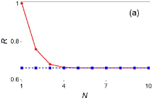
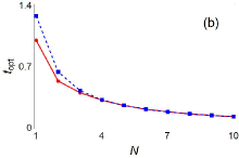
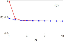
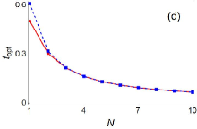
Figure 2: (Color online) The sensitivity ratios $R$ defined by Eq. (25) and the optimal interrogation time $t_{{\rm opt}}$ as a function of the probe number $N$ for the ADC (a, b) and DPC (c, d) cases. Red solid lines correspond to the ancilla-free strategy and blue dashed lines to the ancilla-assisted one.

4 Conclusion

We investigated the frequency sensitivity achievable with generalized GHZ states in the presence of Markovian covariant phase noises, which models a broad family of noises requiring that the processes between the system Hamiltonian and dissipation commute. By invoking the QFI theory, we analytically determined the ultimate sensitivities achievable with the use of ancilla-assisted strategy and the optimal measurement to saturate the sensitivities were also found. In contrast to the ancilla-free strategy, we found that the effect of ancilla-assisted strategy on sensitivity preserving is more pronounced for few number of probes, but become negligible when the probe number is slightly greater. Our results also indicate that taking a single ancillary qubit in ancilla-assisted strategy is sufficient, while using more ancillae will not bring any more benefit to frequency sensitivity.

Appendix A: Calculation of the QFIs

In this appendix, we present detailed derivation of the QFI for ancilla-free and ancilla-assisited frequency estimation strategies with the generalized GHZ states in the presence of phase covariant noises. To facilitate our calculation, we first obtain the analytical expression of the QFI with respect to the phase of $\phi=\omega t$, denoted as $F_{\phi}$. Then the QFI with respect to the frequency can be obtained from $F_{\phi}$ by using the equality of $F_{\omega}=t^{2}F_{\phi}$. In the scenarios discussed in the main text, the phase-encoded density matrices can be always decomposed into a direct sum of two sub-matrices, $\mathcal{E}\left(\rho_{{\rm GHZ}}\right)=\varrho_{\phi}\oplus\varrho_{D}$ with $\phi$-dependent $2\times 2$ dimensional matrices $\varrho_{\phi}$ and $\phi$-independent diagonal matrices $\varrho_{D}$. According to the sum property of the QFI Demkowicz-Dobrzanski2009PRA , i.e., $F_{\phi}=\sum_{\nu}F\left(\varrho_{\nu}\right)$ for $\rho=\bigoplus_{\nu}\varrho_{\nu}$, we find that the QFI of $\mathcal{E}\left(\rho_{{\rm GHZ}}\right)$ is simply given by $F_{\phi}=F\left(\varrho_{\phi}\right)$ due to no contribution from the $\phi$-independent sub-matrix $\varrho_{D}$. Thanks also to the simple form of $\varrho_{\phi}$, that is of dimension only $2$, then its corresponding QFI can be formulated with respect to the Bloch vector $\bm{r}$ of $\varrho_{\phi}$ as Zhong2013PRA

$$F\left(\varrho_{\phi}\right) = \frac{1}{r_{0}}\left[|\partial_{\phi}\bm{r}|^{2}+\frac{\left(\bm{r}\cdotp\partial_{\phi}\bm{r}\right)^{2}}{r_{0}-|\bm{r}|^{2}}\right],$$ (A1)

with the normalization factor $r_{0}={\rm Tr\left(\varrho_{\phi}\right)}$.

At first, we consider the ancilla-free case in which the frequency encoded density matrix is given by Eqs. (10) and (11). By setting $\phi=\omega t$, we write the $\phi$-dependent part as

$$\varrho_{\phi} = \left(\begin{array}[]{cc}2^{-N}\left(\left|c_{1}\right|^{2}A_{++}^{N}+\left|c_{2}\right|^{2}A_{-+}^{N}\right)&c_{1}c_{2}^{\ast}\eta_{\perp}^{N}e^{-iN\left(\theta+\phi\right)}\\ c_{1}^{\ast}c_{2}\eta_{\perp}^{N}e^{iN\left(\theta+\phi\right)}&2^{-N}\left(\left|c_{1}\right|^{2}A_{--}^{N}+\left|c_{2}\right|^{2}A_{+-}^{N}\right)\end{array}\right),\quad\quad$$ (A4)

associating with

$$r_{0} = 2^{-N}\left[\left|c_{1}\right|^{2}\left(A_{++}^{N}+A_{--}^{N}\right)+\left|c_{2}\right|^{2}\left(A_{-+}^{N}+A_{+-}^{N}\right)\right],$$ (A5)

$$\bm{r} = \left(\begin{array}[]{c}2c_{1}c_{2}^{\ast}\eta_{\perp}^{N}\cos N\left(\theta+\phi\right)\\ 2c_{1}c_{2}^{\ast}\eta_{\perp}^{N}\sin N\left(\theta+\phi\right)\\ 2^{-N}\left[\left|c_{1}\right|^{2}\left(A_{++}^{N}-A_{--}^{N}\right)+\left|c_{2}\right|^{2}\left(A_{-+}^{N}-A_{+-}^{N}\right)\right]\end{array}\right).$$ (A9)

By replacing Eq. (A1) with the above $r_{0}$ and $\bm{r}$, one can directly obtain Eq. (12) as a result of $\left(\bm{r}\cdotp\partial_{\phi}\bm{r}\right)^{2}=0$ and $F_{\omega}=t^{2}F_{\phi}$. Similarly, as for the ancilla-assisted case, the $\phi$-dependent sub-density matrix corresponding to Eq. (18) is

$$\varrho_{\phi} = \left(\begin{array}[]{cc}2^{-N}\left|c_{1}\right|^{2}A_{++}^{N}&c_{1}c_{2}^{\ast}\eta_{\perp}^{N}e^{-iN\left(\theta+\phi\right)}\\ c_{1}^{\ast}c_{2}\eta_{\perp}^{N}e^{iN\left(\theta+\phi\right)}&2^{-N}\left|c_{2}\right|^{2}A_{+-}^{N}\end{array}\right),$$ (A12)

equipped with

$$r_{0} = 2^{-N}\left(\left|c_{1}\right|^{2}A_{++}^{N}+\left|c_{2}\right|^{2}A_{+-}^{N}\right),$$ (A13)

$$\bm{r} = \left(\begin{array}[]{c}2c_{1}c_{2}^{\ast}\eta_{\perp}^{N}\cos N\left(\theta+\phi\right)\\ 2c_{1}c_{2}^{\ast}\eta_{\perp}^{N}\sin N\left(\theta+\phi\right)\\ 2^{-N}\left(\left|c_{1}\right|^{2}A_{++}^{N}-\left|c_{2}\right|^{2}A_{+-}^{N}\right)\end{array}\right).$$ (A17)

Submitting these into Eq. (A1), one finally gets Eq. (20) as a consequence of $\left(\bm{r}\cdotp\partial_{\phi}\bm{r}\right)^{2}=0$ and $F_{\omega}=t^{2}F_{\phi}$.

Appendix B: Demonstration of the optimal observable

While the QFI bounds the optimal sensitivity achievable with a given quantum state, the sensitivity is limited by the measurements which can be implemented in the experimental platform. Given a measurement observable $O$, the attainable sensitivity is given by the error-propagation formula

$$\Delta^{2}\hat{\omega}T\geq\frac{\left(\left\langle O^{2}\right\rangle-\left\langle O\right\rangle^{2}\right)}{t\left|\partial\left\langle O\right\rangle/\partial\phi\right|^{2}},$$ (B1)

where the sufficient and necessary condition for an observable $O$ to saturate the QFI bounds was proposed in Zhong2014JPA .

Here, we show that the observable of direct-sum form $O_{A}=\sigma_{x}\oplus\bm{1}$ with $\sigma_{x}$ acting on the subspace of the density matrix corresponding to $\varrho_{\phi}$ and $\bm{1}$ on the residual subspace corresponding to $\varrho_{D}$, is an optimal measurement for both ancilla-free and ancilla-assisted strategies discussed in the main text. Let us take the ancilla-free strategy for example. The expectation values of the first and second moments of $O$ in $\varrho_{\phi}\oplus\varrho_{D}$ can be easily calculated as

$$\left\langle O\right\rangle = 2\left|c_{1}\right|\left|c_{2}\right|\eta_{\perp}^{N}\sin N\left(\theta+\phi\right),$$ (B2)

$$\left\langle O^{2}\right\rangle = \left|c_{1}\right|^{2}\left(A_{++}^{2}+A_{--}^{2}\right)+\left|c_{2}\right|^{2}\left(A_{-+}^{2}+A_{+-}^{2}\right).$$ (B3)

Submitting the above results into Eq. (B1) yields

$$\Delta^{2}\hat{\omega}T\geq\frac{\left(\left|c_{1}\right|^{2}\left(A_{++}^{2}+A_{--}^{2}\right)+\left|c_{2}\right|^{2}\left(A_{-+}^{2}+A_{+-}^{2}\right)-4\left|c_{1}\right|^{2}\left|c_{2}\right|^{2}\eta_{\perp}^{2N}\sin^{2}N\left(\theta+\phi\right)\right)}{4t\left|c_{1}\right|^{2}\left|c_{2}\right|^{2}\eta_{\perp}^{2N}N^{2}\cos N\left(\theta+\phi\right)}.$$ (B4)

Hence it meets the sensitivity bounds given by Eq. (12) under the condition of $N\left(\theta+\phi\right)=2k\pi,k\in\mathbb{Z}$.

References

- (1) Wineland, D. J., Bollinger, J. J., Itano, W. M., and Heinzen, D. J.: Squeezed atomic states and projection noise in spectroscopy. Phys. Rev. A 50, 67 (1994)
- (2) Bollinger, J. J, Itano, Wayne M., Wineland, D. J., and Heinzen, D. J.: Optimal frequency measurements with maximally correlated states. Phys. Rev. A 54, R4649 (1996)
- (3) Leibfried, D., Barrett, M. D., Schaetz, T., Britton, J., Chiaverini, J., Itano, W. M., Jost, J. D., Langer, C., and Wineland, D.: Toward Heisenberg-Limited Spectroscopy with Multiparticle Entangled States. Science 304, 5676 (2004)
- (4) Taylor, J. M., Cappellaro, P., Childress, L., Jiang, L., Budker, D., Hemmer, P. R., Yacoby, A., Walsworth, R., and Lukin, M. D.: High-sensitivity diamond magnetometer with nanoscale resolution. Nat. Phys. 4, 10 (2008)
- (5) Goldstein, G., Cappellaro, P., Maze, J. R., Hodges, J. S., Jiang, L., Srensen, A. S., and Lukin, M. D.: Environment-Assisted Precision Measurement. Phys. Rev. Lett. 106, 140502 (2011)
- (6) Collaboration, LIGO Scientific: A gravitational wave observatory operating beyond the quantum shot-noise limit. Nat. Phys. 7, 962 (2011)
- (7) Collaboration, LIGO Scientific: Enhanced sensitivity of the LIGO gravitational wave detector by using squeezed states of light. Nat. Photon. 7, 613 (2013)
- (8) Barsotti, Lisa, Harms, Jan, and Schnabel, Roman: Squeezed vacuum states of light for gravitational wave detectors. Rep. Prog. Phys. 82, 016905 (2018)
- (9) Halkyard, P. L., Jones, M. P. A., and Gardiner, S. A.: Rotational response of two-component Bose-Einstein condensates in ring traps. Phys. Rev. A 81, 061602 (2010)
- (10) Helm, J. L., Cornish, S. L., and Gardiner, S. A.: Sagnac Interferometry Using Bright Matter-Wave Solitons. Phys. Rev. Lett. 114, 134101 (2015)
- (11) Stevenson, R., Hush, M. R., Bishop, T., Lesanovsky, I., and Fernholz, T.: Sagnac Interferometry with a Single Atomic Clock. Phys. Rev. Lett. 115, 163001 (2015)
- (12) Giovannetti, Vittorio, Lloyd, Seth, and Maccone, Lorenzo: Quantum Metrology. Phys. Rev. Lett. 96, 010401 (2006)
- (13) Giovannetti, Vittorio, Lloyd, Seth, and Maccone, Lorenzo: Advances in quantum metrology. Nat. Photon. 5, 222 (2011)
- (14) Frwis, F. and Dür, W.: Stable Macroscopic Quantum Superpositions. Phys. Rev. Lett. 106, 110402 (2011)
- (15) Ma, Jian, Huang, Yi-Xiao, Wang, Xiao-Guang, and Sun, C. P.: Quantum Fisher information of the Greenberger-Horne-Zeilinger state in decoherence channels. Phys. Rev. A 84, 022302 (2011)
- (16) Chaves, Rafael, Aolita, Leandro, and Acín, Antonio: Robust multipartite quantum correlations without complex encodings. Phys. Rev. A 86, 020301 (2012)
- (17) Zhong, Wei, Sun, Zhe, Ma, Jian, Wang, Xiaoguang, and Nori, Franco: Fisher information under decoherence in Bloch representation. Phys. Rev. A 87, 022337 (2013)
- (18) Huelga, S. F., Macchiavello, C., Pellizzari, T., Ekert, A. K., Plenio, M. B., and Cirac, J. I.: Improvement of Frequency Standards with Quantum Entanglement. Phys. Rev. Lett. 79, 3865 (1997)
- (19) Escher, B. M., de Matos Filho, R. L., and Davidovich, L.: General framework for estimating the ultimate precision limit in noisy quantum-enhanced metrology. Nat. Phys. 7, 406 (2011)
- (20) Demkowicz-Dobrzanski, Rafal, Kolodynski, Jan, and Guta, Madalin: The elusive Heisenberg limit in quantum-enhanced metrology. Nat. Commun. 3, 1063 (2012)
- (21) Dür, W., Skotiniotis, M., Fröwis, F., and Kraus, B.: Improved Quantum Metrology Using Quantum Error Correction. Phys. Rev. Lett. 112, 080801 (2014)
- (22) Arrad, G., Vinkler, Y., Aharonov, D., and Retzker, A.: Increasing Sensing Resolution with Error Correction. Phys. Rev. Lett. 112, 150801 (2014)
- (23) Kessler, E. M., Lovchinsky, I., Sushkov, A. O., and Lukin, M. D.: Quantum Error Correction for Metrology. Phys. Rev. Lett. 112, 150802 (2014)
- (24) Lu, Xiao-Ming, Yu, Sixia, and Oh, C. H.: Robust quantum metrological schemes based on protection of quantum Fisher information. Nat. Commun. 6, 7282 (2015)
- (25) Herrera-Martí, David A., Gefen, Tuvia, Aharonov, Dorit, Katz, Nadav, and Retzker, Alex: Quantum Error-Correction-Enhanced Magnetometer Overcoming the Limit Imposed by Relaxation. Phys. Rev. Lett. 115, 200501 (2015)
- (26) Unden, Thomas, Balasubramanian, Priya, Louzon, Daniel, Vinkler, Yuval, Plenio, Martin B., Markham, Matthew, Twitchen, Daniel, S¡: Quantum Metrology Enhanced by Repetitive Quantum Error Correction. Phys. Rev. Lett. 116, 230502 (2016)
- (27) Layden, David, Zhou, Sisi, Cappellaro, Paola, and Jiang, Liang: Ancilla-Free Quantum Error Correction Codes for Quantum Metrology. Phys. Rev. Lett. 122, 040502 (2019)
- (28) Sekatski, Pavel, Skotiniotis, Michalis, Koodyński, Janek, and Dür, Wolfgang: Quantum metrology with full and fast quantum control. Quantum 1, 27 (2017)
- (29) Sekatski, Pavel, Skotiniotis, Michalis, and Dür, Wolfgang: Dynamical decoupling leads to improved scaling in noisy quantum metrology. New J. Phys. 18, 073034 (2016)
- (30) Tan, Qing-Shou, Huang, Yi-Xiao, Yin, Xiao-Lei, Kuang, Le-Man, and Wang, Xiao-Guang: Enhancement of parameter-estimation precision in noisy systems by dynamical decoupling pulses. Phys. Rev. A 87, 032102 (2013)
- (31) Gammelmark, Sren and Mlmer, Klaus: Bayesian parameter inference from continuously monitored quantum systems. Phys. Rev. A 87, 032115 (2013)
- (32) Gammelmark, Sren and Mlmer, Klaus: Fisher Information and the Quantum Cramér-Rao Sensitivity Limit of Continuous Measurements. Phys. Rev. Lett. 112, 170401 (2014)
- (33) Catana, Catalin and Guţǎ, Mǎdǎlin: Heisenberg versus standard scaling in quantum metrology with Markov generated states and monitored environment. Phys. Rev. A 90, 012330 (2014)
- (34) Kiilerich, Alexander Holm and Mlmer, Klaus: Estimation of atomic interaction parameters by photon counting. Phys. Rev. A 89, 052110 (2014)
- (35) Kiilerich, Alexander Holm and Mlmer, Klaus: Bayesian parameter estimation by continuous homodyne detection. Phys. Rev. A 94, 032103 (2016)
- (36) Plenio, Martin B. and Huelga, Susana F.: Sensing in the presence of an observed environment. Phys. Rev. A 93, 032123 (2016)
- (37) Cortez, Luis, Chantasri, Areeya, García-Pintos, Luis Pedro, Dressel, Justin, and Jordan, Andrew N.: Rapid estimation of drifting parameters in continuously measured quantum systems. Phys. Rev. A 95, 012314 (2017)
- (38) Chase, Bradley A. and Geremia, J. M.: Single-shot parameter estimation via continuous quantum measurement. Phys. Rev. A 79, 022314 (2009)
- (39) Stockton, John K., Geremia, J. M., Doherty, Andrew C., and Mabuchi, Hideo: Robust quantum parameter estimation: Coherent magnetometry with feedback. Phys. Rev. A 69, 032109 (2004)
- (40) Geremia, JM, Stockton, John K., Doherty, Andrew C., and Mabuchi, Hideo: Quantum Kalman Filtering and the Heisenberg Limit in Atomic Magnetometry. Phys. Rev. Lett. 91, 250801 (2003)
- (41) Albarelli, Francesco, Rossi, Matteo A. C., Paris, Matteo G. A., and Genoni, Marco G.: Ultimate limits for quantum magnetometry via time-continuous measurements. New J. Phys. 91, 123011 (2017)
- (42) Demkowicz-Dobrza n šœski, Rafal and Maccone, Lorenzo: Using Entanglement Against Noise in Quantum Metrology. Phys. Rev. Lett. 113, 250801 (2014)
- (43) Huang, Zixin, Macchiavello, Chiara, and Maccone, Lorenzo: Usefulness of entanglement-assisted quantum metrology. Phys. Rev. A 94, 012101 (2016)
- (44) Huang, Zixin, Macchiavello, Chiara, and Maccone, Lorenzo: Noise-dependent optimal strategies for quantum metrology. Phys. Rev. A 97, 032333 (2018)
- (45) Sbroscia, Marco, Gianani, Ilaria, Mancino, Luca, Roccia, Emanuele, Huang, Zixin, Maccone, Lorenzo, Macchiavello, Chiara, and Ba¡: Experimental ancilla-assisted phase estimation in a noisy channel. Phys. Rev. A 97, 032305 (2018)
- (46) Wang, Kunkun, Wang, Xiaoping, Zhan, Xiang, Bian, Zhihao, Li, Jian, Sanders, Barry C., and Xue, Peng: Entanglement-enhanced quantum metrology in a noisy environment. Phys. Rev. A 97, 042112 (2018)
- (47) Smirne, Andrea, Koody n šœski, Jan, Huelga, Susana F., and Demkowicz-Dobrza n šœski, Rafa: Ultimate Precision Limits for Noisy Frequency Estimation. Phys. Rev. Lett. 116, 120801 (2016)
- (48) Helstrom, C. W.: Quantum Detection and Estimation Theory. Academic. New York(1976)
- (49) Holevo, A. S.: Probabilistic and Statistical Aspects of Quantum Theory. North-Holland. Amsterdam(1982)
- (50) Braunstein, Samuel L. and Caves, Carlton M.: Statistical distance and the geometry of quantum states. Phys. Rev. Lett. 72, 3439 (1994)
- (51) James, Daniel F. V., Kwiat, Paul G., Munro, William J., and White, Andrew G.: Measurement of qubits. Phys. Rev. A 64 052312 (2001)
- (52) Romero, K M Fonseca and Franco, R Lo: Simple non-Markovian microscopic models for the depolarizing channel of a single qubit. Phys. Scr. 86, 065004 (2012)
- (53) Demkowicz-Dobrzanski, R., Dorner, U., Smith, B. J., Lundeen, J. S., Wasilewski, W., Banaszek, K., and Walmsley, I. A.: Quantum phase estimation with lossy interferometers. Phys. Rev. A 80, 013825 (2009)
- (54) Zhong, Wei, Lu, Xiao Ming, Jing, Xiao Xing, and Wang, Xiao Guang: Optimal condition for measurement observable via error-propagation. J. Phys. A: Math. Theor. 47, 385304 (2014)