A Distributed Multi-Robot Coordination Algorithm for Navigation in Tight Environments

Abstract

This work presents a distributed method for multi-robot coordination based on nonlinear model predictive control (NMPC) and dual decomposition. Our approach allows the robots to coordinate in tight spaces (e.g., highway lanes, parking lots, warehouses, canals, etc.) by using a polytopic description of each robot’s shape and formulating the collision avoidance as a dual optimization problem. Our method accommodates heterogeneous teams of robots (i.e., robots with different polytopic shapes and dynamic models can be part of the same team) and can be used to avoid collisions in $n$-dimensional spaces. Starting from a centralized implementation of the NMPC problem, we show how to exploit the problem structure to allow the robots to cooperate (while communicating their intentions to the neighbors) and compute collision-free paths in a distributed way in real time. By relying on a bi-level optimization scheme, our design decouples the optimization of the robot states and of the collision-avoidance variables to create real time coordination strategies. Finally, we apply our method for the autonomous navigation of a platoon of connected vehicles on a simulation setting. We compare our design with the centralized NMPC design to show the computational benefits of the proposed distributed algorithm. In addition, we demonstrate our method for coordination of a heterogeneous team of robots (with different polytopic shapes).

I INTRODUCTION

Autonomous robots will soon be part of our daily lives [1]. The automotive industry is investing billions in self-driving technologies [2], maritime-transportation companies are already developing autonomous boats [3], and retail companies are investing in autonomous warehouse robots [4]. These technologies have the potential to reduce fatalities, transportation efficiency, and the overall quality of life [5].

To fully exploit the benefits that these technologies will bring, algorithms to control and efficiently coordinate these autonomous robots are crucial, especially in tight environments (e.g., highway lanes, parking lots, warehouses, canals, etc.), where the robots have reduced maneuver space. To reach their goals, each robot closely interacts with its neighbors to avoid collisions. Hence, one of the challenges to ensure safe navigation of connected autonomous robots is that of efficiently generating a safe coordination strategy. Multi-robot systems are the focus of our paper. In particular, w focus on efficient, safe and coordinated multi-robot trajectory planning (the interested reader can refer to [6] for an overview of the state of the art)

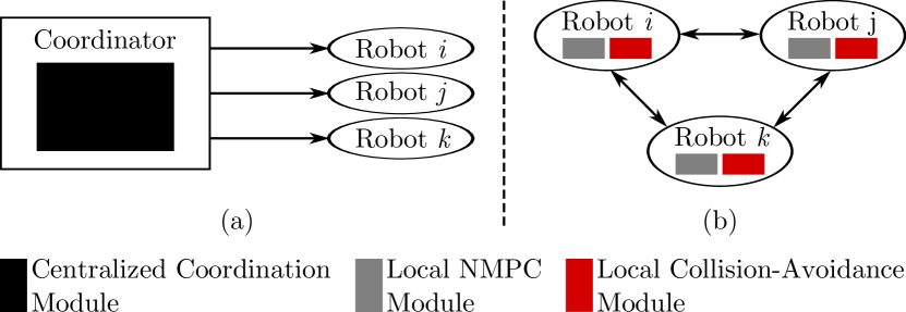
Figure 1: Centralized design (a) vs. our distributed design (b) for multi-robot coordination.

Contribution. We use a nonlinear model predictive control (NMPC) to plan collision-free trajectories to coordinate the robots. We use a polytopic representation of the individual robot and formulate the collision avoidance problem as the problem of finding the minimum distance between two polytopes. To incorporate this collision avoidance strategy in the NMPC formulation, our method relies on duality theory [7]. We reformulate the minimum distance collision-avoidance constraints between each pair of robots as a feasibility test (with associated collision-avoidance variables) that can be included within the constraints of the NMPC problem. Solving the NMPC problem in a centralized way (Fig. 1.a) is computationally intensive, so we introduce an algorithm to solve the NMPC problem in a distributed way (Fig. 1.b), which is computationally efficient compared to centralized formulation and is suitable for real time applications.

In order to split the centralized problem into distributed sub-problems, the centralized formulation must be separable. Although the dynamic models of the robots are decoupled, but the collision avoidance constraints are coupled among them. To break the coupling, we rely on a bi-level optimization approach to decompose the centralized problem as local minimization problems performed by alternating between two different optimizations (Fig. 1.b): (i) a collision avoidance optimization (red boxes in Fig. 1.b) that computes the predicted collision-avoidance variables, given the latest predicted intention of each pair of robots, and (ii) local NMPC optimizations (grey boxes in Fig. 1.b) that update the robot states, given the latest predicted collision-avoidance variables. The advantage of this decomposition is that each collision avoidance optimization solves efficiently (in milliseconds) convex problems of fixed dimension and the local NMPC problems have always a fixed number of decision variables (the local robot states), compared to the centralized problem. Also we quantify the error caused by relying on open-loop predicted trajectories of neighbor robots in distributed approach. We show that this error is bounded (and small) and we propose a strategy to account for this error in the local NMPC problem formulation. Finally, we validate our method for the autonomous navigation of a platoon of connected vehicles on a highway setting comparing its performance with a centralized implementation. In platooning both road geometry and platoon geometry restrict the motion of the vehicles within the platoon. Hence, the vehicles must coordinate in a tight environment. To allow navigation at tight spaces, our approach models the road structure and the vehicles dimensions, as exact sizes with no approximation or enlargement. We also demonstrate the results for a coordination scenario of a heterogeneous team of robots with different polytopic shapes.

Related Work. Classical methods for multi-robot coordination either use reactive strategies (such as potential fields [8, 9, 10], dynamic window [11], and velocity obstacles [12, 13]), assume a priority order [14], or rely on a scheduling [15] for the robots. These methods, however, do not explicitly consider the interaction among the robots. Learning-based methods [16, 17, 18, 19, 20] and constrained-optimization approaches can be used to take these interactions into account. Our work fits in this last category and relies on tools from control and optimization to model the interactions among the robots to avoid collisions. Distributed constrained-optimization designs have been proposed for example in [21, 22, 23, 24, 25, 26]. The authors in [21] present a decentralized model predictive control (MPC) formulation for multi-robot coordination that relies on invariant-set theory and mix-integer linear programming (MILP). The authors in [22] propose a distributed MPC design for formation control using the alternating direction method of multipliers (ADMM) and separating hyperplanes for collision avoidance. The authors in [23] use a potential cost function and collision-avoidance constraints to formulate a distributed MPC problem, in which the collision avoidance constraints can be either linearized or formulated using integer variables. In addition, the authors rely on motion primitives to account for robot kinematic and dynamic constraints. The authors in [24, 25] present distributed MPC approaches that rely on ADMM to decompose the (linearized) coordination problem. The authors in [26] propose a distributed nonlinear MPC formulation with nonconvex collision avoidance constraints.

Compared to  [21], our proposed approach does not require the solution of a MILP problem that can be computationally expensive to solve. In addition, compared to  [23, 24, 25] our method does not require any linearization (which could reduce the solution space of the problem) of the collision-avoidance constraints. Also compared to  [23], our approach does not require the use of motion primitives (the robot dynamics are directly included in the NMPC formulation). Compared to  [22], our strategy allows to specify a desired distance between the robots, instead of using separating hyperplanes. Inspired by [7, 27], our method uses dual optimization to formulate the collision avoidance constraints. Compared to [7, 27], however, our method exploits the structure of the coordination problem to solve it in a distributed fashion.

Outline. Sec. II provides the required preliminary definitions. Sec. III describes the centralized design. Sec. IV details our distributed algorithm. Sec. V introduces our applications and the simulation results. Sec. VI provides a bound on the prediction error which is a source of discrepancy between centralized and distributed approaches. Sec. VII concludes this paper.

II PRELIMINARIES

We provide the needed definitions and notations below.
Robots and Neighbor Robots: The set of $M$ cooperative robots is defined as $\mathcal{V}:=\{1,2,...,M\}$. We identify each robot through its index $i\in\mathcal{V}$. Throughout this paper, the superscript $i$ denotes the $i$th robot. The neighbor set of robot $i$ is denoted as $\mathcal{N}_{i}$ and represents all the robots that are in the communication range of Robot $i$.
Polytopic Description of Robot Pose: Robot pose or the region occupied by the robot can be described as a convex set defined by a polytope $\mathcal{P}$. Polytopes are described as the intersection of a set of half-spaces and are defined as a set of linear inequalities. The initial pose of the robot is represented as $\mathcal{P}_{o}$. As the robot travels, $\mathcal{P}_{o}$ undergoes affine transformations including rotation and translation. Hence $\mathcal{P}=\mathbf{R}\mathcal{P}_{o}+\mathbf{t}_{r}$, where $\mathbf{R}:\mathbb{R}^{n_{z}}\rightarrow\mathbb{R}^{n\times n}$ is an orthogonal rotation matrix, $\mathbf{t}_{r}:\mathbb{R}^{n_{z}}\rightarrow\mathbb{R}^{n}$ is the translation vector, $n_{z}$ is the dimension of the robot state $\mathbf{z}$, and $n$ is dimension of the space which is 2 for 2D- and 3 for 3D planning.
Static and Dynamic Obstacles: $\mathcal{S}=\{1,...,n_{\mathcal{S}}\}$ is the set of $n_{\mathcal{S}}$ static obstacles. $\mathcal{O}^{r}$ is the $r$-th static obstacle, $r\in\mathcal{S}$. Each static obstacle is modeled as a polytopic set. The collision avoidance between robot $i$ and static obstacle $r$ is defined as $\mathcal{P}^{i}\cap\mathcal{O}^{r}=\emptyset$. $\mathcal{N}_{i}$ is the set of dynamic obstacles for robot $i$. To avoid collision between Robots $i$ and $j$, the intersection of their polytopic sets must be empty, $\mathcal{P}^{i}\cap\mathcal{P}^{j}=\emptyset$.
MPC Scheme: MPC is useful for online local motion planing in uncertain and dynamic environment because it is able to re-plan according to the new available information. MPC relies on the receding-horizon principle. At each time step it solves a constrained optimization problem and obtains a sequence of optimal control inputs that minimize a desired cost function $J$, while considering dynamic, state, and input constraints, over a fixed time horizon. Then, the controller applies, in closed-loop, the first control-input solution. At the next time step, the procedure is repeated. Throughout this paper, $(\cdot|t)$ indicates the values along the entire planning horizon $N$, predicted based on the measurements at time $t$. For example $\mathbf{z}(\cdot|t)$ represents the entire state trajectory along the horizon $[\mathbf{z}(1),\mathbf{z}(2),...,\mathbf{z}(N)]$ predicted at time $t$. The bar notation ($\mathbf{\bar{\cdot}}$) represents constant known values.
MPC Cost Function $J$: The MPC cost is $J:=\sum_{i\in\mathcal{V}}J^{i}$, where $J^{i}$ is the local objectives of each robot. Each $J^{i}$ can be designed according to the local-robot planning and control objectives. For example, the local costs can be specified to reach a goal set or to reduce the deviation from a global reference path (which is not collision-free) computed using high-level planning methods (e.g., A* or RRT*) as proposed in [28, 29, 30, 31] for single-robot local motion planning.

III CENTRALIZED COORDINATION

The multi-robot coordination can be considered as a motion-planning problem and formulated as a centralized MPC optimization problem that computes collision-free trajectories for all the robots, simultaneously. The optimization problem is formulated in the NMPC framework as follows

$$\min_{\begin{subarray}{c}\mathbf{u}^{i}(\cdot|t)\end{subarray}} \sum_{i=1}^{M}J^{i}(\mathbf{z}^{i},\mathbf{u}^{i})$$ (1a)

subject to $$\mathbf{z}^{i}(k+1|t)=f(\mathbf{z}^{i}(k|t),\mathbf{u}^{i}(k|t)),$$ (1b)

$$\mathbf{z}^{i}(0|t)=\mathbf{z}^{i}(t),$$ (1c)

$$\mathbf{z}^{i}(k|t)\in\mathcal{Z},\ \mathbf{u}^{i}(k|t)\in\mathcal{U},$$ (1d)

$$\mathcal{P}(\mathbf{z}^{i}(k|t))\cap\mathcal{O}^{r}=\emptyset,\ r\in\mathcal{S},$$ (1e)

$$\mathcal{P}(\mathbf{z}^{i}(k|t))\cap\mathcal{P}(\mathbf{z}^{j}(k|t))=\emptyset,\quad i\neq j$$ (1f)

$$\forall i\in\mathcal{V},\ j\in\mathcal{N}_{i},{\textrm{and~{}}k\in\{1,2,..,N\}}.$$

In the formulation above, $\mathbf{u}^{i}(\cdot|t)=[u^{i}(k|t),...,u^{i}(k+N-1|t)]$ denotes the sequence of control inputs over the MPC planning horizon $N$ for $i$th robot. $\mathbf{z}^{i}(k|t)$ and $\mathbf{u}^{i}(k|t)$ variables of $i$th robot at step $k$ are predicted at time $t$. The function $f(\cdot)$ in (1b) represents the nonlinear (dynamic or kinematic) model of the robot, which is discretized using Euler discretization. $\mathcal{Z}$, $\mathcal{U}$ are the state and input feasible sets, respectively. These sets represent state and actuator limitations. Constraints (1f) represent the collision-avoidance constraints between the $i$th robot and all the neighboring robots within the communication radius. This representation is time-varying and is a function of the robot state at each time step. The remainder of this section details the derivation of constraints (1e) and (1f). Note that the centralized NMPC problem (1), might get infeasible. However, persistent feasibility of (1) can be guaranteed by computing the reachable set. In this paper, our focus is to reformulate the centralized problem (1) into a distributed one, but the techniques to guarantee persistent feasibility can be incorporated into our proposed approach.

III-A Collision Avoidance Reformulation

Consider two polytopic sets $\mathcal{P}_{1}$ and $\mathcal{P}_{2}$. The distance between these sets is given by the following primal problem

$$\text{dist}(\mathcal{P}_{1},\mathcal{P}_{2})=\underset{{\mathbf{x},\mathbf{y}}}{\min}\{\|\mathbf{x}-\mathbf{y}\|_{2}|\mathbf{A}_{1}\mathbf{x}\leq\mathbf{b}_{1},\mathbf{A}_{2}\mathbf{y}\leq\mathbf{b}_{2}\},\\$$ (2)

where $\mathcal{P}_{1}=\{\mathbf{x}\in\mathbb{R}^{n}|\mathbf{A}_{1}\mathbf{x}\leq\mathbf{b}_{1}\}$ and $\mathcal{P}_{2}=\{\mathbf{y}\in\mathbb{R}^{n}|\mathbf{A}_{2}\mathbf{y}\leq\mathbf{b}_{2}\}$. The two sets do not intersect if $\text{dist}(\mathcal{P}_{1},\mathcal{P}_{2})>0$. For motion-planning applications, however, the robots must keep a minimum safe distance $d_{\min}$ from each other and from the obstacles. Hence, the distance between their polytopic sets should be larger than a predefined minimum distance, $\text{dist}(\mathcal{P}_{1},\mathcal{P}_{2})\geq d_{\min}.$

Problem (2) is itself an optimization problem that cannot directly be used in Problem (1), because we would have an optimization problem as the constraint of another optimization problem. To deal with this issue, we rely on strong-duality theory. Building on [7], the dual problem can be solved instead of the primal problem (2). The dual problem is expressed as follows:

$$\text{dist}(\mathcal{P}_{1},\mathcal{P}_{2}):= \underset{{\bm{\lambda}_{12},\bm{\lambda}_{21},\,\mathbf{s}}}{\max}-\mathbf{b}_{1}^{\top}\bm{\lambda}_{12}-\mathbf{b}_{2}^{\top}\bm{\lambda}_{21}$$ (3)

$$\text{s.t.~{}}\mathbf{A}_{1}^{\top}\bm{\lambda}_{12}+\mathbf{s}=0,\ \mathbf{A}_{2}^{\top}\bm{\lambda}_{21}-\mathbf{s}=0,$$

$$\quad\ ||\mathbf{s}||_{2}\leq 1,-\bm{\lambda}_{12}\leq 0,\ -\bm{\lambda}_{21}\leq 0,$$

where $\bm{\lambda}_{12}$, $\bm{\lambda}_{21}$ and $\mathbf{s}$ are dual variables (the derivation of (3) from (2) is provided in the Appendix). The optimal value of the dual problem is the distance between $\mathcal{P}_{1}$ and $\mathcal{P}_{2}$ and is constrained to be larger than a desired minimum distance. Consequently, we can use this insight to reformulate the dual problem as the following feasibility problem: $\{\exists\bm{\lambda}_{12}\succeq 0,\bm{\lambda}_{21}\succeq 0,\mathbf{s}:-\mathbf{b}_{1}^{\top}\bm{\lambda}_{12}-\mathbf{b}_{2}^{\top}\bm{\lambda}_{21}\geq d_{\text{min}},\mathbf{A}_{1}^{\top}\bm{\lambda}_{12}+\mathbf{s}=0,\mathbf{A}_{2}^{\top}\bm{\lambda}_{21}-\mathbf{s}=0,\|\mathbf{s}\|_{2}\leq 1\}.$ This reformulation can be substituted to the collision-avoidance constraint (1f) in Problem (1). A similar reformulation can be derived for static obstacles (1e). Therefore, problem (1) can be rewritten as

$$\min_{\begin{subarray}{c}\mathbf{u}^{i}(\cdot|t),\ \bm{\lambda}_{ij}(\cdot|t),\\ \bm{\lambda}_{ji}(\cdot|t),\ \mathbf{s}_{ij}(\cdot|t)\end{subarray}} {\sum_{i=1}^{M}J^{i}(\mathbf{z}^{i},\mathbf{u}^{i})}$$

subject to $${\eqref{eq:dynamic_constraint},\eqref{eq:initial_cond},}{\eqref{eq:state_input_bound},}$$

$${\big{(}-\mathbf{b}^{i}(\mathbf{z}^{i}(k|t))^{\top}}\bm{\lambda}_{ij}(k|t)$$

$$-\mathbf{b}^{j}(\mathbf{z}^{j}(k|t))^{\top}\bm{\lambda}_{ji}(k|t)\big{)}\geq d_{\text{min}},$$ (4a)

$$\mathbf{A}^{i}(\mathbf{z}^{i}(k|t))^{\top}\bm{\lambda}_{ij}(k|t)\!+\!\mathbf{s}_{ij}(k|t)\!=\!0,$$ (4b)

$$\mathbf{A}^{j}(\mathbf{z}^{j}(k|t))^{\top}\bm{\lambda}_{ji}(k|t)\!-\!\mathbf{s}_{ij}(k|t)\!=\!0,$$ (4c)

$${\bm{\lambda}_{ij}(k|t),\bm{\lambda}_{ji}(k|t)\geq 0,\|{\mathbf{s}_{ij}(k|t)}\|_{2}\leq 1,}$$

$${\forall i}{\in\mathcal{V},\ j\in\mathcal{N}_{i},~{}}{\text{and~{}}k\in\{1,2,..,N\},}$$

where $\mathbf{A}^{i}$ and $\mathbf{b}^{i}$ are functions of $\mathbf{z}^{i}(k|t)$ and represent the polytopic set of $i$th vehicle at step $k$ predicted at time $t$. Similarly $\mathbf{A}^{j}$ and $\mathbf{b}^{j}$ denote the polytopic set of $j$th robot which belongs to neighbor set $\mathcal{N}_{i}$. The dual variables $\bm{\lambda}_{ij}$, $\bm{\lambda}_{ji}$ and $\mathbf{s}_{ij}$ are coupled through the collision avoidance constraint between robot $i$ and robot $j$. For space limitation the static obstacle avoidance constraint (1e) is removed in the above formulation and only the collision avoidance among robots are formulated. However, it can be added using dual reformulation. Note that the dual variable $\mathbf{s}_{ij}$ is equivalent to the variable $\mathbf{s}$ in (3). The new variable $\mathbf{s}_{ij}$ is introduced in (4) to distinguish for example, $\mathbf{s}_{12}$ from $\mathbf{s}_{13}$, but $\mathbf{s}_{12}$ is identical to $\mathbf{s}_{21}$ according to (3). Therefore, the variables $\mathbf{s}_{ij}$, $\mathbf{s}_{ji}$ and $\mathbf{s}$ are all identical vectors ($\mathbf{s}_{ij}$ = $\mathbf{s}_{ji}$ = $\mathbf{s}$ $\in\mathbb{R}^{n}$) with dimension of $n$ that is the dimension of the space which is 2 for 2D- and 3 for 3D planning. We will discuss the geometric interpretation of the vector $\mathbf{s}$ in the next section.

Remark III.1.

The required minimum distance between the robots $d_{\text{min}}$, which can be chosen as a design parameter. In theory, the trajectories can be obtained for $d_{\text{min}}=0$, which means the polytopic sets (i.e., the robots) can move on each other boundaries. In practice, $d_{\text{min}}$ should be determined based on the quantification of uncertainty of physical models and stochastic measurement errors.

IV DISTRIBUTED COORDINATION

Problem (4) simultaneously optimizes over all the robots’ states $\mathbf{z}^{i}$ and the collision avoidance variables $\bm{\lambda}_{ij},\bm{\lambda}_{ji},\mathbf{s}_{ij}$ (for all $i=1,...,M$, $j\neq i$), that is, the number of variables to optimize is proportional to the number of robots. This is computationally expensive when $M$ is large, making the centralized formulation not scalable with the number of robots. Our goal is to remove the need of a central coordinator and make the problem scalable with the number of robots (allowing the robots to coordinate and locally solve smaller sub-problems in parallel).

By looking at the structure of Problem (4), we notice that the collision avoidance constraints (4a)-(4c) create a coupling among the robots. In addition, Constraint (4a) creates a nonlinear coupling between the state variables $\mathbf{z}^{i}$,$\mathbf{z}^{j}$ and the collision avoidance variables $\bm{\lambda}_{ij}$,$\bm{\lambda}_{ji}$. To break-up these couplings and devise the proposed distributed algorithm, we rely on the dual structure we originally used to formulate Problem 4 and on the ability of MPC to generate predictions. In particular, our idea is to solve Problem (4) by using a bi-level optimization scheme, that is, we replace the central coordinator by using two independent optimizations that perform alternating optimization of the dual variables (associated with the collision avoidance constraints) and of primal state variables, respectively, as Algorithm 1 details.

In Algorithm 1, first the dual variables over the NMPC horizon are initialized, then the first optimization step (NMPC optimization) optimizes the state variables $\mathbf{z}^{i}$,$\mathbf{z}^{j}$ over the horizon, while keeping the dual variables $\bm{\lambda}_{ij}$,$\bm{\lambda}_{ji},\mathbf{s}_{ij}$ fixed. The second optimization step (CA optimization) optimizes the dual variable while keeping the state variables fixed. We detail these two optimizations below.

IV-A NMPC optimization

At time $t$, each robot $i$ independently computes its own state $\mathbf{z}^{i}$ trajectory, given the dual variables over the horizon $[\bm{\lambda}_{ij}(1)$, $\dots$, $[\bm{\lambda}_{ij}(N)]$, $[\bm{\lambda}_{ji}(1)$, $\dots$, $\bm{\lambda}_{ji}(N)]$ and $[\mathbf{s}_{ij}(1)$, $\dots$, $\mathbf{s}_{ij}(N)]$. For each robot $i\in\mathcal{V},\ j\in\mathcal{N}_{i}$, the NMPC optimization is given by:

$$\min_{\begin{subarray}{c}\mathbf{u}^{i}(\cdot|t)\end{subarray}} {J^{i}(\mathbf{z}^{i},\mathbf{u}^{i})}$$

subject to $${\eqref{eq:dynamic_constraint},\eqref{eq:initial_cond},\eqref{eq:state_input_bound}},$$

$${\big{(}-\mathbf{b}^{i}(\mathbf{z}^{i}(k|t))^{\top}\bm{\bar{\lambda}}_{ij}(k|t)}$$

$$-\mathbf{\bar{b}}^{j}(\mathbf{\bar{z}}^{j}(k|t))^{\top}\bm{\bar{\lambda}}_{ji}(k|t)\big{)}\geq d_{\text{min}},$$ (5a)

$$\mathbf{A}^{i}(\mathbf{z}^{i}(k|t))^{\top}\bm{\bar{\lambda}}_{ij}(k|t)+\mathbf{\bar{s}}_{ij}(k|t)=0,$$ (5b)

$${\text{for all }k\in\{1,2,..,N\}},$$

where the bar notation ($\mathbf{\bar{\cdot}}$) represents constant known values and $\mathbf{A}^{i}$, $\mathbf{b}^{i}$ are the polytopic representation of the $i$th robot and are functions of $\mathbf{z}^{i}$. The optimized trajectory is then shared with the collision avoidance optimization (shifted in time according to step \footnotesize{5}⃝ of Algorithm 1 to account for the 1-step delay in the calculation of the collision-avoidance strategies). Problem (5) can be solved in parallel by each robot. In this optimization, the collision-avoidance variables $\bm{\lambda}_{ij},\bm{\lambda}_{ji},\mathbf{s}_{ij}$ are considered as known values along the planning horizon. Note that compared to the centralized formulation, the only decision variable to optimize in the NMPC optimization is the $i$th robot state $\mathbf{z}^{i}$ (i.e., the number of decision variables in the local problem formulations is constant).

IV-B Collision Avoidance (CA) optimization

Each robot pair of $i,j\in\mathcal{N},\ i\neq j$, computes the collision avoidance variables $\bm{\lambda}_{ij},\bm{\lambda}_{ji},\mathbf{s}_{ij}$. The CA optimization is given by

$$\max_{\begin{subarray}{c}\bm{\lambda}_{ij}(\cdot|t),\\ \bm{\lambda}_{ji}(\cdot|t),\\ \mathbf{s_{ij}}(\cdot|t)\end{subarray}} \!\!\!\!\!\!\!\!\!-\!{\mathbf{\bar{b}}^{i}\!(\mathbf{\bar{z}}^{i}(k|t))^{\top}\!\bm{\lambda}_{ij}(k|t)\!-\!\mathbf{\bar{b}}^{j}\!(\mathbf{\bar{z}}^{j}(k|t))^{\top}\!\bm{\lambda}_{ji}(k|t)}$$

subject to $$\mathbf{\bar{A}}^{i}(\mathbf{\bar{z}}^{i}(k|t))^{\top}\bm{\lambda}_{ij}(k|t)+\mathbf{s}_{ij}(k|t)=0,$$ (6a)

$$\mathbf{\bar{A}}^{j}(\mathbf{\bar{z}}^{j}(k|t))^{\top}\bm{\lambda}_{ji}(k|t)-\mathbf{s}_{ij}(k|t)=0,$$ (6b)

$${\big{(}-\mathbf{\bar{b}}^{i}(\mathbf{\bar{z}}^{i}(k|t))^{\top}\bm{\lambda}_{ij}(k|t)}$$

$${-\mathbf{\bar{b}}^{j}(\mathbf{\bar{z}}^{j}(k|t))^{\top}\bm{\lambda}_{ji}(k|t)\big{)}\geq d_{\text{min}},}$$

$$\|{\mathbf{s}_{ij}(k|t)}\|_{2}\leq 1,-\bm{\lambda}_{ij}(k|t)\leq 0,$$ (6c)

$${-\bm{\lambda}_{ji}(k|t)\!\leq\!0,\ \text{for all }\!i\!\in\!\mathcal{V},\ j\!\in\!\mathcal{N}_{i},}$$

$${\text{for all }k\in\{1,2,..,N\}.}$$

Each robot solves Problem (6) in parallel. This optimization assumes the state trajectories of the robots $\mathbf{z}^{i}$ to be fixed (obtained by the NMPC optimization and from the neighboring robots according to step \footnotesize{7}⃝ of Algorithm 1). This problem can be solved efficiently (in the order of milliseconds).

Algorithm 1 is a bi-level optimization scheme with the NMPC optimization (5) as the upper-level optimization problem and the CA optimization (6) as the lower-level optimization problem. On one hand this bi-level optimization scheme allows us to improve computation time of coordination strategy. On the other hand, due to this optimization scheme, the distributed NMPC (5) returns less tight trajectories (larger margins in the coordination) compared to the centralized NMPC (4). Solving lower-level CA optimization and substituting its solution in the upper-level NMPC optimization further restricts the constraints (5a)-(5b), since the dual variables are kept fixed (i.e., the NMPC optimizer has less degree of freedom in the computation of the local trajectories). In contrast, in the centralized NMPC (4), the equivalent constraints (4a)-(4c) can be interpreted as the relaxed version of the constraints (5a)-(5b), since the dual variables are decision variables of the centralized problem.

Algorithm 1 Distributed Coordination Algorithm

1:Initialize $[\mathbf{s}_{ij}(1),...,\!\mathbf{s}_{ij}(N)],$ $[\bm{\lambda}_{ij}(1),...,\bm{\lambda}_{ij}(N)],$ $[\bm{\lambda}_{ji}(1),...,\bm{\lambda}_{ji}(N)]$, $\forall i,j\in\mathcal{N}$ and $i\neq j.$

2:for  $t=0,1,...,\infty$ do

3:    for all Robot $i$, $i\in\mathcal{V}$ do in parallel

4:         Solve Problem (5)

5:         Compute the shifted state $[\mathbf{z}^{i}(2),...,\mathbf{z}^{i}(N),\mathbf{z}^{i}(N)]$.

6:         Compute the associated polytopic sets: $[\mathbf{A}^{i}(2),...,$ zzzzzzz$\mathbf{A}^{i}(N),$ $\mathbf{A}^{i}(N)]$, $[\mathbf{b}^{i}(2),$…, $\mathbf{b}^{i}(N),$ $\mathbf{b}^{i}(N)].$

7:         Communicate to Robot $j$ ($\forall j\in\mathcal{N}_{i}$) the polytopic sets.

8:         Solve Problem (6) for each $j\in\mathcal{N}_{i}$

9:         Apply $\mathbf{u}_{\text{MPC}}^{i}$ to move forward.

10:    end for

11:end for

IV-C Geometric Interpretation of Primal and Dual Variables

The dual variables have an interesting geometric interpretation. All these geometric meanings are obtained from the Karush–Kuhn–Tucker (KKT) conditions for problem (2) and more details can be found in  [32]. As seen in Fig. 2, the top plots show the geometric representation of the primal formulation (2) in which the optimal solutions are $\mathbf{x}^{*}$ and $\mathbf{y}^{*}$ and the distance is defined as the classical Euclidean distance $\|\mathbf{x}^{*}-\mathbf{y}^{*}\|_{2}$ between the two sets. The bottom plots show the equivalent dual formulation (3) in which the optimal solutions are $\mathbf{s}^{*}$, $\bm{\lambda}_{12}^{*}$ and $\bm{\lambda}_{21}^{*}$ and the same distance between the two polytopic sets is defined as $-{\mathbf{b}_{1}}^{\top}\bm{\lambda}_{12}^{*}-{\mathbf{b}_{2}}^{\top}\bm{\lambda}_{21}^{*}$. As Fig. 2(e) depicts, the separating hyperplane between the two polytopic sets is always perpendicular to the minimum distance. Therefore $\mathbf{s}^{*}$, which is the normal vector of the separating hyperplane, is always parallel to the minimum distance. The normal vector $\mathbf{s}^{*}$ plays the role of the consensus variable between the robots. As discussed earlier, the vector $\mathbf{s}^{*}$ is shared between each pair of robots according to (3), so $\mathbf{s}_{ij}=\mathbf{s}_{ji}$. Furthermore, in Fig. 2(f), the green lines show the two supporting hyperplanes which are parallel to the separating hyperplane. The hyperplane $\mathbf{s}^{*}{{}^{\top}}\mathbf{x}=-\mathbf{b}_{1}^{\top}\bm{\lambda}^{*}_{12}$ supports the set $\mathbf{x}$ or $(\mathcal{P}_{1})$ at the point $\mathbf{x}^{*}$. Similarly the hyperplane $\mathbf{s}^{*}{{}^{\top}}\mathbf{y}=\mathbf{b}_{2}^{\top}\bm{\lambda}^{*}_{21}$ supports the set $\mathbf{y}$ or $(\mathcal{P}_{2})$ at the point $\mathbf{y}^{*}$. On the other hand, the primal (2) and dual (3) problems are convex and the Slater’s condition is satisfied, so the strong duality holds [33]. Therefore, finding the shortest distance between two polytopic sets (primal problem (2)) is equivalent to finding the maximal separation, which is the maximum distance between a pair of parallel hyperplanes that supports the two sets (dual problem (3)) as shown in Fig. 2(f).

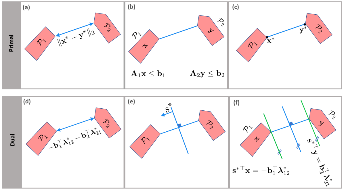
Figure 2: Top: Primal (a) minimum distance (b) polytope representation (c) optimal solutions. Bottom: Dual: (d) minimum distance (e) separating hyperplane (f) supporting hyperplanes.

V NUMERICAL RESULTS FOR AUTONOMOUS DRIVING APPLICATION

In this section we compare the centralized and distributed approaches in terms of computation time (and cost) as the number of robots increase. Section V-A describes the simulation setup. Sections V-B and V-C presents two different simulation scenarios, that are, a) a platoon formation and re-configuration and b) a heterogeneous team of robots with different polytopic shapes, respectively.

V-A Simulation Setup

We tested our design on a quad-core CPU Intel Core i7-7700HQ @ 2.80 GHz in MATLAB using the MATLAB Parallel Computing Toolbox to simulate the individual robots and communication exchanges among the robots. We modeled the optimization problems in YALMIP [34]. We solved Problems (4), (5) using IPOPT [35], a state-of-the-art interior-point solver for non-convex optimization, and we solved Problem (6) using Gurobi [36], an efficient QP problem. For all the scenarios the simulation results are presented as top view snapshots, as well as a series of state and action plots. The robots colors of the snapshots and plots are matched.

V-B Platoon Formation

1 In this scenario, autonomous and connected vehicles merge into a platoon (train-like formation) and maintain a close inter-vehicular distance within the group. In platooning on public roads, both road geometry (lane width) and platoon geometry (longitudinal and lateral inter-vehicle spacing) restrict the motion of the vehicles within the platoon. Hence, the vehicles must coordinate in a tight environment. To allow navigation at tight spaces, it is essential to model the road structure and the vehicles dimensions, including length $h$ and width $w$, as exact sizes with no approximation or enlargement.

V-B1 Relevant NMPC Quantities

We model each vehicle $i$ within the platoon by using a nonlinear kinematic bicycle model (a common modeling approach in path planning) described by the following equations [37] (we omit the superscript $i$ when it is clear from the context):

$$\dot{x} =v\cos(\psi+\beta),\ \dot{y}=v\sin(\psi+\beta),$$ (7)

$$\dot{\psi} =\frac{v\cos\beta}{l_{f}+l_{r}}(\tan\delta),\ \dot{v}=a,$$

where the $i$th vehicle state vector is $\mathbf{z}=[x,y,\psi,v]^{\top}$ ($x$, $y$, $\psi$, and $v$ are the longitudinal position, the lateral position, the heading angle, and the velocity, respectively), the control input vector is $\mathbf{u}=[a,\delta]^{\top}$ ($a$ and $\delta$ are the acceleration and the steering angle, respectively), $\beta:=\arctan\big{(}\tan\delta(\frac{l_{r}}{l_{f}+l_{r}})\big{)}$ is the side slip angle, and $l_{f}$, $l_{r}$ are the distance from the center of gravity to the front and rear axles, respectively. Using Euler discretization, the model (7) is discretized with sampling time $\Delta t$ as

$$x(t+1) =x(t)+\Delta t\ v(t)\cos(\psi(t)+\beta(t)),$$ (8)

$$y(t+1) =y(t)+\Delta t\ v(t)\sin(\psi(t)+\beta(t)),$$

$$\psi(t+1) =\psi(t)+\Delta t\ \frac{v(t)\cos\beta(t)}{l_{f}+l_{r}}(\tan\delta(t)),$$

$$v(t+1) =v(t)+\Delta t\ a(t).$$

The local costs are defined as $J(\mathbf{z},\mathbf{u})$ $=\sum_{k=t}^{t+N}$ $\|(\mathbf{z}(k|t)$ $-\mathbf{z}_{\textrm{Ref}}(k|t))\|^{2}_{Q_{\mathbf{z}}}$ $+\sum_{k=t}^{t+N-1}$ $(\|(\mathbf{u}(k|t))||^{2}_{Q_{\mathbf{u}}}$ $+\|$ $(\Delta\mathbf{u}(k|t))\|^{2}_{Q_{\bm{\Delta u}}})$, where $\Delta\mathbf{u}$ penalizes changes in the input rate. $Q_{\mathbf{z}}\succeq 0$, $Q{{}_{\mathbf{u}}},Q_{\bm{\Delta u}}\succ 0$ are weighting matrices, $\mathbf{z}_{\textrm{Ref}}$ is the reference trajectory generated by a high-level planner (and it is not obstacle-free). The $i$th vehicle dimensions are chosen as length $h=4.5$m and width $w=1.8$m. The road width is chosen as $3.7$m (i.e., the standard highway-lane width in the United States). The speed is lower bounded by zero. The acceleration of each vehicle is bounded within $\pm\,4$m/s² and its rate change is bounded within $\pm\,1$m/s². The steering input is bounded within $\pm\,0.3$rad and its change within $\pm 0.2$rad/s. The corresponding road region occupied by the $i$th vehicle is defined by a two-dimensional convex polytope $\mathcal{P}.$ For each vehicle, the transformed polytope is defined as $\mathcal{P}(\mathbf{z}(t))=\{p\in\mathbb{R}^{2}|\mathbf{A}(\mathbf{z}(t))p\leq\mathbf{b}(\mathbf{z}(t))\},$ where $\mathbf{A}(\mathbf{z}(t))$ and $\mathbf{b}(\mathbf{z}(t))$ are defined as $\mathbf{A}(\mathbf{z}(t))=\begin{bmatrix}\mathbf{R}(\mathbf{z}(t))^{\top}\\ -\mathbf{R}(\mathbf{z}(t))^{\top}\end{bmatrix},\ \mathbf{R}(\mathbf{z}(t))=\begin{bmatrix}\cos(\psi(t))&-\sin(\psi(t))\\ \sin(\psi(t))&\cos(\psi(t))\end{bmatrix},$ $\mathbf{b}(\mathbf{z}(t))=[h/2,w/2,h/2,w/2]^{\top}$ $+\mathbf{A}(\mathbf{z}(t))[x(t),y(t)]^{\top}$, where $[x(t),y(t)]^{\top}$ is the center of gravity of the vehicle.

V-B2 Platoon Formation Results

In this scenario, as seen in Fig. 3(a), the vehicles are initially traveling in three different lanes and need to merge in one lane to form a train-like platoon, while maintaining the safe distance $d_{min}=0.5$m from each other at all times (i.e., during the lane change maneuvers and afterwards). We tested the formation scenario for different configurations and initial conditions. Fig. 3(b) shows an example with four vehicles. The initial longitudinal coordinates for all the four vehicles are $[x^{1}(0),x^{2}(0),x^{3}(0),x^{4}(0)]=[11.5,5.5,0.5,20]$ and the initial lateral coordinates are $[y^{1}(0),y^{2}(0),y^{3}(0),y^{4}(0)]=[1.85,5.55,1.85,9.25]$. The planning horizon $N$ is $0.75$s, the sampling time $\Delta t$ is $0.05$s, and $v_{\text{Ref}}$ is $15$m/s. Fig. 3(b) represents the vehicles’ states and actions. The longitudinal and lateral coordinates $x$ and $y$, as well as heading angle $\psi$ and velocity $v$ for all the vehicles are shown in different colors which are matched with the colors in Fig. 3(a).

The control actions $a$ and $\delta$ are also illustrated for all the vehicles. The acceleration and velocity plots highlights the collaborative behavior between the vehicles. In contrast to reactive approaches, such as velocity obstacles, the speed of each vehicle is not assumed constant and varies based on the interactions with the neighbors. For example, as seen in the acceleration plot, the blue vehicle brakes and the magenta vehicle accelerates to make enough gap for other vehicles to merge into the lane. This behavior is obtained by the solving the optimization problem and is not enforced explicitly. This collaborative behavior is fundamental to keep the desired minimum distance and form the platoon. Ellipsoidal representations of the vehicles would have required a larger minimum distance (to fit each vehicle the axes of each ellipses would have been 6.36m and 2.54m, respectively, leading to a minimum distance, in the longitudinal direction for example, equal to ($2(6.36-4.5)$m$>d_{\min}$) leading to more conservative behaviors. Similar considerations hold for implementations based on potential fields. A potential field can be always included in the NMPC problem formulation to enforce clearance with respect to the other vehicles, but it would lead to more conservative behaviors (e.g., larger minimum distance between the vehicles) and additional tuning parameters. In Fig. 3(a)(a), in addition to snapshots, the separating hyperplanes between pink/green, green/red and red/blue pairs are shown and the normal of these separating hyperplanes are denoted as $\mathbf{s}_{pg}$, $\mathbf{s}_{gr}$ and $\mathbf{s}_{rb}$, respectively.

To evaluate the performance in terms of computation time of Algorithm 1, we simulated the formation of two, three and four vehicles in highway (varying the initial configuration of the vehicles to test the robustness of the tuning). We compared the average and maximum computation time in second for each step along the trajectory with the centralized implementation. Table I shows the results. While both centralized and distributed approaches ensure safe robot coordination, the maximum and average of computation time for centralized approach increases dramatically by adding a vehicle ($>>N$), compromising the safety of the approach in real-time applications (i.e., delays in the calculation of the planning strategy can lead to collisions). The distributed approach outperforms the centralized design by more than 2 orders of magnitude (when we look at the worst case scenario with 4 vehicles) and the computation time is reasonable for online implementation ($<<N$). In addition, Table II compares the sum of closed-loop costs for centralized and distributed approaches. The simulation has been performed for two, three and four coordinated vehicles. The average of cost has increased using distributed approach compared to centralized approach. Based on the results of Table I and Table II, there is a trade-off between computation time and cost of deviation from the reference trajectory.

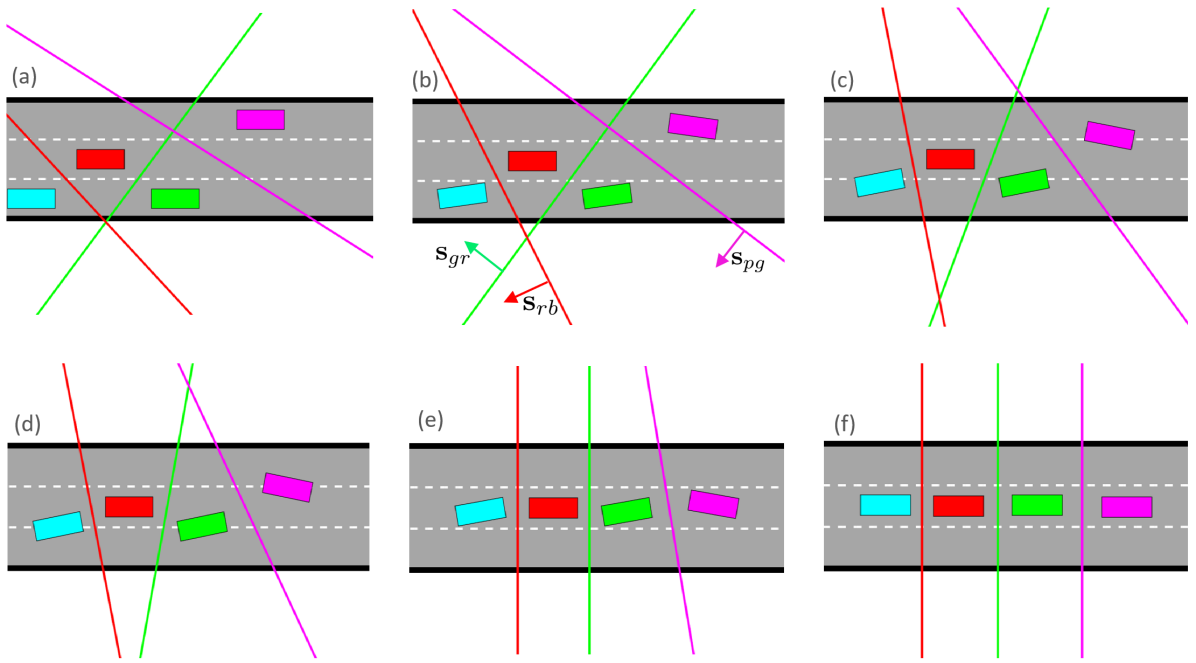
(a) Snapshots

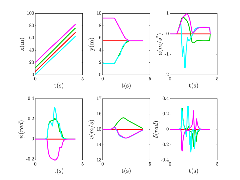
(b) Vehicles trajectories

Figure 3: Four vehicles merge into a platoon in the center lane. The direction of motion is to the right. (a) Snapshots of the simulation are shown with the separating hyperplanes between the vehicles. (b) The state and input trajectories are shown.

	Centralized		Distributed
			NMPC		CA
#	Avg.	Max.	Avg.	Max.	Avg.	Max.
2	1.3851	2.7482	0.1457	0.3621	0.0022	0.0024
			0.1102	0.3313	0.0021	0.0022
			Total Avg. = 0.1301
3	2.7680	4.6817	0.1848	0.3933	0.0025	0.0028
			0.1206	0.3169	0.0024	0.0026
			0.1416	0.3470	0.0022	0.0023
			Total Avg. = 0.1514
4	12.8331	28.7763	0.1919	0.4211	0.0030	0.0024
			0.1125	0.2602	0.0027	0.0029
			0.1842	0.3497	0.0024	0.0025
			0.2041	0.4195	0.0025	0.0023
			Total Avg. = 0.1757

TABLE I: Computation time (in second) for both centralized and distributed approaches are reported for two, three and four numbers of coordinated vehicles.

	Centralized	Distributed
#	Sum of Costs	Sum of Costs
2	0.0443	1.8957
		1.6845
		Total Avg. = 1.7901
3	0.0985	6.0267
		0.0000
		5.6856
		Total Avg. = 3.9041
4	0.0321	6.8064
		0.0000
		12.1444
		10.3252
		Total Avg. = 7.3190

TABLE II: The total cost (sum of the closed-loop costs for the entire maneuver) is reported for centralized and distributed approaches for two, three and four numbers of coordinated vehicles.

V-C Heterogeneous Robots Reconfiguration and Tight Collision Avoidance

We consider a team of robots with different polytopic shapes as seen in Fig. 4. The robots are initially in a circular formation. A goal region is assigned to each robot. The robots should plan their motion based on the shared information communicated from other robots to reach their goals while avoiding collision with each other.

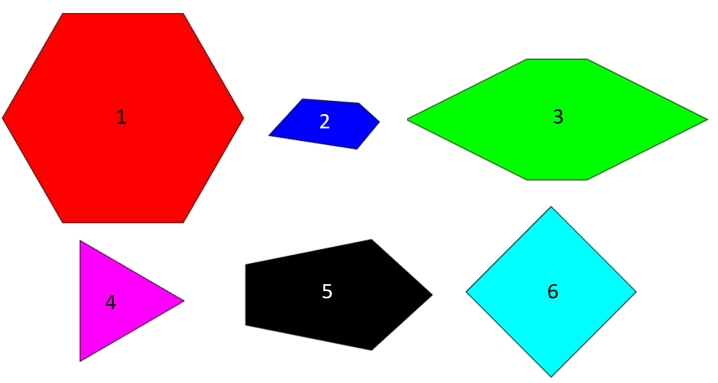
Figure 4: Polytopic Shapes

V-C1 Relevant Problem Parameters

Each robot $i$ is modeled by a nonlinear kinematic unicycle model which is similar to the previously described model (7)

$$\dot{x} =v\cos(\psi),\ \dot{y}=v\sin(\psi),\ \dot{\psi}=\delta,$$ (9)

where the $i$th robot state vector is $\mathbf{z}=[x,y,\psi]^{\top}$ and the control input vector is $\mathbf{u}=[v,\delta]^{\top}$ (the notations are the same as model (7). Using Euler discretization, the model (9) is discretized with sampling time $\Delta t$ as

$$x(t+1) =x(t)+\Delta t\ v(t)\cos(\psi(t)),$$ (10)

$$y(t+1) =y(t)+\Delta t\ v(t)\sin(\psi(t)),$$

$$\psi(t+1) =\psi(t)+\Delta t\ \delta(t),$$

The local costs are defined as $J(\mathbf{z},\mathbf{u})$ $=\sum_{k=t}^{t+N}$ $\|(\mathbf{z}(k|t)$ $-\mathbf{z}_{\textrm{Goal}})\|^{2}_{Q_{\mathbf{z}}}$ $+\sum_{k=t}^{t+N-1}$ $(\|(\mathbf{u}(k|t))||^{2}_{Q_{\mathbf{u}}}$ $+\|$ $(\Delta\mathbf{u}(k|t))\|^{2}_{Q_{\bm{\Delta u}}})$, where $\Delta\mathbf{u}$ penalizes changes in the input rate. $Q_{\mathbf{z}}\succeq 0$, $Q{{}_{\mathbf{u}}},Q_{\bm{\Delta u}}\succ 0$ are weighting matrices, $\mathbf{z}_{\textrm{Goal}}$ is the goal location that robot should reach.

The sampling time is 0.05s, minimum allowable distance $d_{\text{min}}$ is $10$cm, the velocity input is bounded within $\pm\,4$m/s and its rate change is bounded within $\pm\,0.5$m/s. The rate change of steering input is bounded within $\pm\,0.5$rad/s. The $i$th robot shape is defined by a two-dimensional convex polytope centered at the origin $\mathcal{P}_{O}=\{p\in\mathbb{R}^{2}|\mathbf{A}_{O}\ p\leq\mathbf{b}_{O}\}$. As the robot moves, the polytopic shape undergoes rotation and translation. The transformed polytope is defined as $\mathcal{P}(\mathbf{z}(t))=\{p\in\mathbb{R}^{2}|\mathbf{A}(\mathbf{z}(t))p\leq\mathbf{b}(\mathbf{z}(t))\},$ where $\mathbf{A}(\mathbf{z}(t))$ and $\mathbf{b}(\mathbf{z}(t))$ are defined as $\mathbf{A}(\mathbf{z}(t))=\mathbf{A}_{O}\mathbf{R}(\mathbf{z}(t))^{\top},\ \mathbf{R}(\mathbf{z}(t))=\begin{bmatrix}\cos(\psi(t))&-\sin(\psi(t))\\ \sin(\psi(t))&\cos(\psi(t))\end{bmatrix},$ $\mathbf{b}(\mathbf{z}(t))=\mathbf{b}_{O}$ $+\mathbf{A}(\mathbf{z}(t))[x(t),y(t)]^{\top}$, where $[x(t),y(t)]^{\top}$ is the center of gravity of the vehicle.

V-C2 Heterogeneous Robots Reconfiguration Results

Six robots with different polytopic shapes are considered as shown in Fig. 7 (a). A square (light blue), a hexagon (red), an irregular pentagon (dark blue), a hexagon (green), a triangle (pink), a pentagon (black) are representation of the robots and are located on a circle. The goal assigned to each robot is the other end of the diameter of the circle (i.e., each robot needs to swap its position with the one of the robot on the opposite side of the circle). For example in Fig. 7 (a), the goal for the red robot is the location of pink robot on the circle. So the pairs on the same diameter swap their locations. The pairs red/pink, dark blue/black and green/light blue swap, respectively, as shown in Fig. 5. The Fig. 5 shows the position of each robot along the simulation in x-y plane. The Fig. 6 shows the control input trajectories and the Fig. 7 shows the snapshots of the simulation. The initial formation of robots is shown in snapshot (a), then (b)-(e) snapshots shown how they resolve the conflict among each other and (f) shows the final configuration, in which the pairs have swapped their locations. As seen, the robots reduce their speed to avoid collisions at the center of the circle. The open-loop predicted trajectories are shown with small circles for each robot.

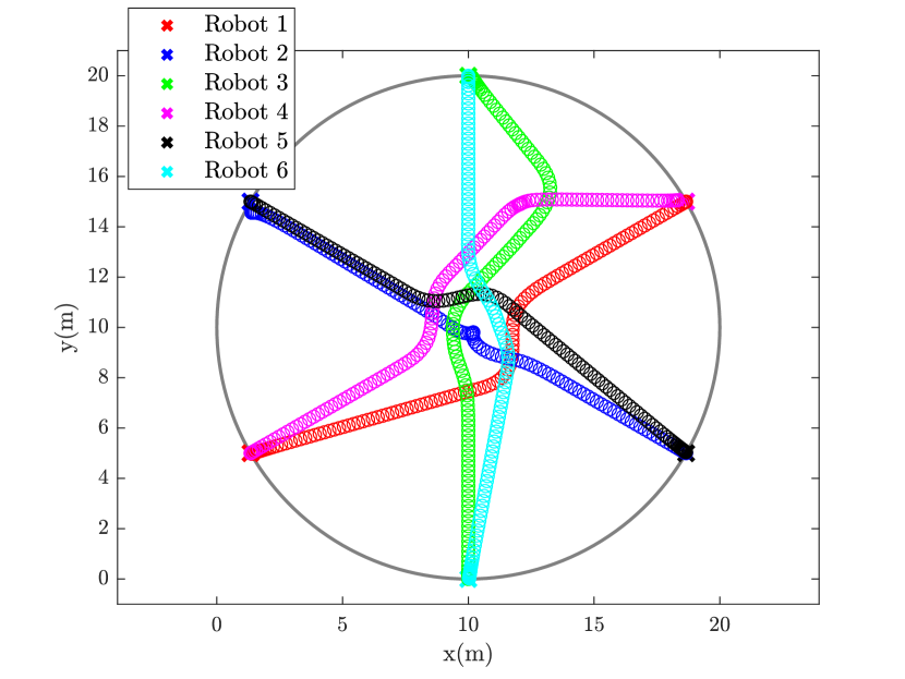
Figure 5: Trajectories of all the robots in x-y plane.

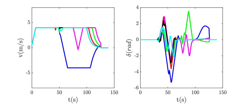
Figure 6: Control input trajectories of the six robots.

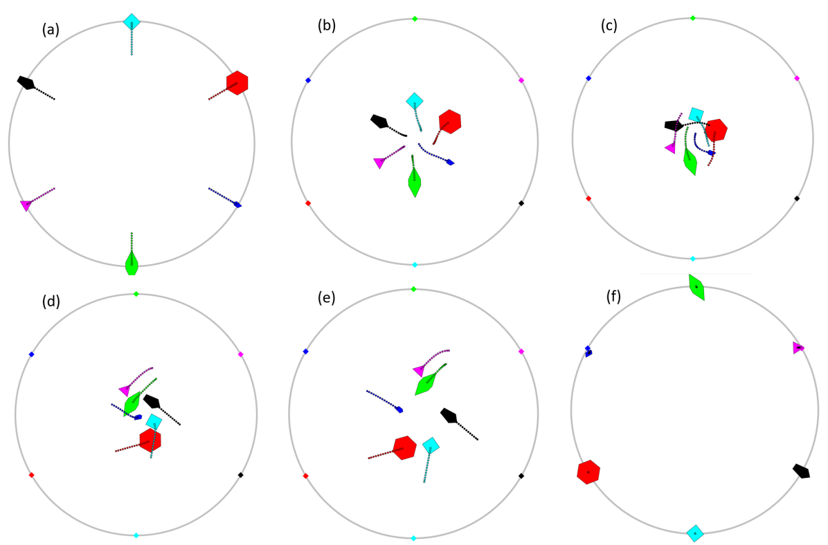
Figure 7: Snapshots of the reconfiguration of a team of 6 heterogeneous robots with different polytopic shapes are shown. The predicted open-loop trajectories are shown with small dots.

Remark V.1.

Note that the proposed coordination strategy is a local one and the performance can be affected by choosing different tuning parameters. For example, choosing a short planning horizon (which would help reduce the computation time even further) can cause deadlock situations, which can be preventable by increasing the horizon length. In addition, our design requires communication among the robots and can tolerate delays up to the prediction horizon of the local NMPC formulations. If the delay is exceeded, fallback strategies are required (e.g., rely on local perception to understand the intentions of the neighboring robots or detect possible faults). These strategies, however, are outside the scope of this paper.

VI Prediction Error Bound

In this section we focus on the discrepancy between distributed and centralized approaches caused by trajectory prediction error. In the centralized approach (1), since the coordinator chooses the optimal action for all the robots simultaneously, the approach does not rely on the open-loop trajectories of the neighbor robots (no communication is involved). However, in the distributed problem (5), each robot optimizes its own action based on the communicated information about the predicted (open-loop) trajectories of other robots. In this section, we quantify the trajectory prediction error and establish an upper bound on this error. To help the discussion, we consider a simple simulation scenario and presents all the results for this scenario. In this scenario two cars, namely, car $i$ and car $j$, are moving in the same direction using two different lanes when car $i$ decides to overtake and merge into car $j$’s lane, as shown in Fig. 8, (for more details on the model and formulation refer to Sec. V-B).

Consider the open-loop trajectory of robot $i$ predicted by robot $i$ as $\bm{\tau}^{i}_{pi}(t)=[\mathbf{z}^{i}(0|t),\mathbf{z}^{i}(1|t),\dotsc,\mathbf{z}^{i}(N|t)]$ and the shifted and augmented open-loop trajectory of robot $i$ predicted by robot $j$ as $\bm{\bar{\tau}}^{i}_{pj}(t-1)=[\mathbf{\bar{z}}^{i}(1|t-1),\mathbf{\bar{z}}^{i}(2|t-1),\dotsc,\mathbf{\bar{z}}^{i}(N|t-1),\mathbf{\bar{z}}^{i}(N|t-1)]$, (the trajectory is shifted one step forward in time and augmented with the same last value). The subscript $pi$ means predicted by robot $i$ and similarly $pj$ means predicted by robot $j$. Also $\bm{\tau}^{j}_{pj}(t)$ represents trajectory of robot $j$ predicted by $j$ at current time step $t$ and $\bm{\bar{\tau}}^{i}_{pj}(t-1)$ denotes the trajectory of robot $i$ predicted by robot $j$ at the previous time step $t-1$.

The prediction error at each time step $t$, $e_{\text{predict}}(t)$ is defined as

$$e_{\text{predict}}(t)=\|\text{dist}_{pi}(t)-\text{dist}_{pj}(t)\|_{2},$$ (11)

where $\text{dist}_{pi}$ is the distance between robot $i$ and robot $j$ predicted by robot $i$ (distance from the point of view of robot $i$) and, similarly, $\text{dist}_{pj}$ is the distance between robot $i$ and robot $j$ predicted by robot $j$ (distance from the point of view of robot $j$). The predicted distances are equivalent to

$$\text{dist}_{pi}(t) \simeq\|\bm{\tau}^{i}_{pi}(t)-{\bm{\bar{\tau}}}^{j}_{pi}(t-1)\|_{2},$$ (12)

$$\text{dist}_{pj}(t) \simeq\|\bm{\tau}^{j}_{pj}(t)-{\bm{\bar{\tau}}}^{i}_{pj}(t-1)\|_{2},$$

and by substituting (12) in (11), the predicted error is equivalent to

$$e_{\text{predict}}(t)\simeq$$ (13)

$$\|\bigg{(}\|\bm{\tau}^{i}_{pi}(t)-{\bm{\bar{\tau}}}^{j}_{pi}(t-1)\|_{2}-\|\bm{\tau}^{j}_{pj}(t)-{\bm{\bar{\tau}}}^{i}_{pj}(t-1)\|_{2}\bigg{)}\|_{2}.$$

Since the cars are rigid bodies (modeled as polytopic sets) and not just point masses, we consider the exact minimum distance between the two polytopic sets and define $\text{dist}_{pi}$ and $\text{dist}_{pj}$ using the notion of distance between the sets. As discussed earlier, the distance between the two polytopic sets $i$ and $j$ is defined as $-{\mathbf{b}^{i}}^{\top}\bm{\lambda}_{ij}-{\mathbf{b}^{j}}^{\top}\bm{\lambda}_{ji}$. However this value is different from the view of robot $i$ and robot $j$, in distributed approach ($\text{dist}_{pi}\neq\text{dist}_{pj}$). According to distance constraint (5a), we have

$$\text{dist}_{pi}(t)=-{\mathbf{b}^{i}}(t)^{\top}\bm{\bar{\lambda}}_{ij}(t-1)-{\mathbf{\bar{b}}^{j}}(t-1)^{\top}\bm{\bar{\lambda}}_{ji}(t-1),$$ (14)

$$\text{dist}_{pj}(t)=-{\mathbf{\bar{b}}^{i}}(t-1)^{\top}\bm{\bar{\lambda}}_{ij}(t-1)-{\mathbf{b}^{j}}(t)^{\top}\bm{\bar{\lambda}}_{ji}(t-1)$$ (15)

By substituting (14) and (15) in (11), the prediction error $e_{\text{predict}}$ can be computed. After this quantification, we establish an upper-bound on the prediction error. Note that in the centralized approach, the prediction error $e_{\text{predict}}$ is zero since no communication is involved (the approach does not rely on the open-loop trajectory predictions of other robots) and $\text{dist}_{pi}=\text{dist}_{pj}$.

Theorem 1.

Let the minimum distance between robot $i$ and $j$ from the perspective of robot $i$ and $j$ be defined according to (14) and (15), respectively. By using Algorithm 1 to solve Problem (5), the prediction error is bounded, that is,

$$e_{\textrm{predict}}(t) =\|\textrm{dist}_{pi}(t)-\textrm{dist}_{pj}(t)\|_{2}$$ (16)

$$\leq c_{i}||\mathbf{b}^{i}(\mathbf{z}^{i}(t))-\bar{\mathbf{b}}^{i}(\bar{\mathbf{z}}^{i}(t-1))||_{2}$$

$$+c_{j}||\mathbf{b}^{j}(\mathbf{z}^{j}(t))-\mathbf{\bar{b}}^{j}(\mathbf{\bar{z}}^{j}(t-1))||_{2},$$

where $c_{i}$ and $c_{j}$ are constant scalars. For vehicle applications with rectangular polytopic shapes $c_{i}$ and $c_{j}$ are equal to one. For general polytopic shapes $c_{i}=\sqrt{2}\|({\mathbf{A}_{O}}^{i{\top}})^{\dagger}\|_{\mathbf{F}}=\sqrt{2\sum_{i=1}^{r}\sigma_{i}^{2}}$, where $\sigma_{i}$ is the $i$th singular value of the matrix and $r$ is its rank. Similarly, $c_{j}$ has the same definition associated with matrix $(\mathbf{A}_{O}^{j{\top}})^{\dagger}$.

Proof.

See Appendix.

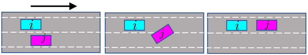
Figure 8: Overtaking maneuver: the top arrow indicates direction of motion.

To clarify the meaning of this time-varying upper-bound (right-hand side of (16)), the overtaking scenario in Fig. 8 is simulated and the minimum distances between the cars at each time step along the simulation is shown in Fig. 9 top plot. As seen in the top plot, $\text{dist}_{pi}$, the distance predicted by car $i$ (light blue line) is different from $\text{dist}_{pj}$, the distance predicted by car $j$ (pink line). The true distance is the actual distance between the cars (gray line). This difference in predicted distances is the prediction error which is bounded according to (16). The bottom plot in Fig. 9, shows that for overtaking scenario the prediction error $e_{\text{predict}}$ (blue line) is bounded by the computed proposed upper bound (right-hand side of (16)) (red line). This upper bound means the prediction error in computing the distance between two cars is bounded by the deviation of the $\mathbf{b}^{i}$ and $\mathbf{b}^{j}$ vectors, between two iterations of the distributed algorithm. The distance in dual formulation is proportional to $\mathbf{b}^{i}$ and $\mathbf{b}^{j}$, which are right-hand side of polytopic set representation, as shown Fig. 2. The error is bounded and it is small, since the vector $\mathbf{b}$ does not change dramatically between two problem iterations.

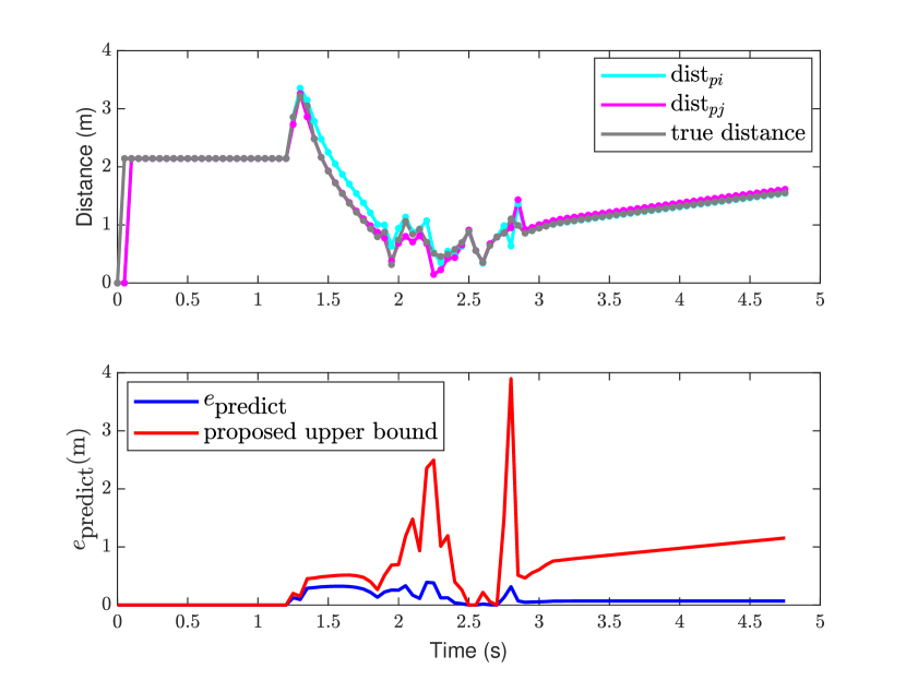
Figure 9: Top In distributed approach, the distance between robot $i$ and robot $j$ from the view of both robots is not the same. Bottom The proposed upper-bound of (16) is illustrated in red for the overtaking simulation and the prediction error on distance is bounded by the proposed upper-bound.

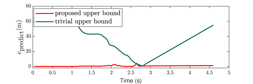
Figure 10: The trivial upper-bound is compared versus the proposed upper-bound on distance error.

In the remainder of this section, we will address the following questions:

1. How tight is this bound compared to a trivial upper bound (computed from boundaries of the feasible set)?

2. For a given acceptable error on the states, how one can rewrite the upper-bound as a function of acceptable error on the states and enforce it as a constraint in NMPC problem (5)?

3. How can one normalize the upper-bound values?

1) To study how tight the upper-bound (16) is, we have compared it with a trivial upper-bound. The trivial upper-bound is defined by maximizing the right-hand-side of (16). This maximization is done by substituting maximum boundary values of the feasible set $\mathcal{Z}$ in (14) and (15). The results for the same overtaking simulation is shown in Fig. 10. The top plot shows that prediction error is bounded by the proposed upper-bound. The bottom plot shows that the proposed upper-bound is considerably tighter than the trivial upper-bound.

2) For a given acceptable error on the states, we can define a threshold for the upper-bound and include the upper-bound (16) in the NMPC formulation (5) to bound the prediction error in the distributed problem. For our application, the states are $x$,$y$ and $\psi$. The maximum error on $x$, $y$ and $\psi$ are denoted as $e_{x}$, $e_{y}$ and $e_{\psi}$, respectively and defined as

$$e_{x} =|x(t)-\bar{x}(t-1)|$$ (17)

$$e_{y} =|y(t)-\bar{y}(t-1)|$$

$$e_{\psi} =|\psi(t)-\bar{\psi}(t-1)|$$

Corollary 1.1.

Given the acceptable error values on the states $e_{x}$, $e_{y}$ and $e_{\psi}$, let $e_{x}$, $e_{y}$ and $e_{\psi}$ be defined as (17), one can compute $\alpha_{\text{min}}\geq 0$, such that the following holds for all $t\geq 0$:

$$||\mathbf{b}^{i}(\mathbf{z}^{i}(t))-\bar{\mathbf{b}}^{i}(\bar{\mathbf{z}}^{i}(t-1))||_{2}\leq\alpha_{\text{min}}(t).$$ (18)

Then by enforcing (18) as a constraint in the NMPC problem (5), if the problem (5) is feasible, the prediction error for each state will not violate the acceptable specified error.

Proof.

To quantify the equation (16) based on acceptable error we have

$$||\mathbf{b}^{i}(\mathbf{z}^{i}(t))-\bar{\mathbf{b}}^{i}(\bar{\mathbf{z}}^{i}(t-1))||_{2}$$ (19)

$$= ||\mathbf{A}(\psi(t))\begin{bmatrix}x(t)\\ y(t)\end{bmatrix}-\mathbf{A}(\bar{\psi}(t-1))\begin{bmatrix}\bar{x}(t-1)\\ \bar{y}(t-1)\end{bmatrix}||_{2}$$

$$= ||\mathbf{A}(\bar{\psi}(t-1)\pm e_{\psi})\begin{bmatrix}\bar{x}(t-1)\pm e_{x}\\ \bar{y}(t-1)\pm e_{y}\end{bmatrix}$$

$$-\mathbf{A}(\bar{\psi}(t-1))\begin{bmatrix}\bar{x}(t-1)\\ \bar{y}(t-1)\end{bmatrix}||_{2}=\alpha(t).$$

We minimize the right-hand side of (19) (all the values are known but different combinations of signs must be considered to find the minimum $\alpha(t)$), then we compare the upper-bound with the threshold value $\alpha_{\text{min}}(t)$

3) To correlate the upper-bound values with specified acceptable predicted error, the upper-bound is normalized by $\alpha_{\text{min}}(t)$. For the overtaking simulation scenario, the acceptable errors are specified as $e_{x}=1$, $e_{y}=0.5$, and $e_{\psi}=0.2$ and $\alpha_{\text{min}}(t)$ is computed from (19) and then the upper-bound is normalized by $\alpha_{\text{min}}$, this normalization ratio $\frac{||\mathbf{b}^{i}(\mathbf{z}^{i}(t))-\bar{\mathbf{b}}^{i}(\bar{\mathbf{z}}^{i}(t-1))||}{\alpha_{\text{min}}}$ is shown in Fig. 11. The prediction error increases as the ratio gets closer to one and decreases as the ratio gets closer to zero. This ratio can be penalized in the cost function in (5) to keep the prediction error close to the acceptable range specified by design engineer.

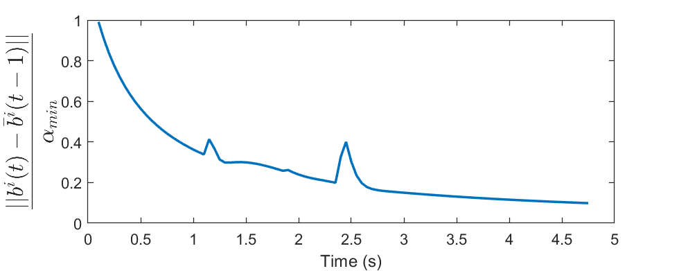
Figure 11: The ratio of upper-bound with respect to $\alpha$ is shown.

VII CONCLUSIONS

We proposed a distributed algorithm for multi-robot coordination in tight spaces using nonlinear MPC and strong duality theory. We reformulated the collision avoidance constraints in dual formulation and used dual decomposition to split the large centralized optimization problem into smaller sub-problems. Our distributed approach consists of upper-level NMPC optimization and lower-level collision avoidance optimization and the algorithm iterate between theses two optimizations in a bi-level optimization scheme.

We showed the effectiveness of the algorithm for coordination of connected and automated vehicles on public roads through platoon merging. We showed the distributed approach outperforms the centralized design by more than 2 orders of magnitude. Our results show that the distributed algorithm is computationally efficient for online implementation and is scalable to larger networks of robots. In addition, we showed the method is generalizable to heterogeneous team of robots with different polytopic shapes. We showed that compared to a centralized design, the proposed decomposition introduces a local prediction error that could lead to more conservative local trajectories. Nevertheless, we proved that this error is bounded and can be accounted for in the local NMPC problems.

As part of our future work, we plan testing with real hardware (e.g., drones and ground vehicles) and in more complex scenarios (e.g., urban driving). From the algorithm-design perspective, we plan to investigate strategies to deal with real sensor data, communication delays, and random faults.

VIII APPENDIX

VIII-A Proof of Theorem 1

Proof.

For robot $i$ and robot $j$, since $\mathbf{s}_{ij}$ represents the consensus variable between the two robots (normal of a separating hyperplane between the robots), therefore $\mathbf{s}_{ij}=\mathbf{s}_{ji}$, in CA optimization (6). Also, based on (6a) and (6b) constraints in CA optimization (6), we have

$$\bm{\lambda}_{ij}=-(\bar{\mathbf{A}}^{i}(\bar{\mathbf{z}}^{i})^{\top})^{\dagger}\mathbf{s}_{ij},$$ (20)

$$\bm{\lambda}_{ji}=(\bar{\mathbf{A}}^{j}(\bar{\mathbf{z}}^{j})^{\top})^{\dagger}\mathbf{s}_{ij},$$ (21)

where $\mathbf{A}^{\dagger}$ is $(\mathbf{A}^{\top}\mathbf{A})^{-1}\mathbf{A}^{\top}$.

The minimum distance $\text{dist}_{pi}$ from the view of robot $i$, is computed by substituting (20) and (21) into (5a)

$$\text{dist}_{pi}=\bigg{(}\mathbf{b}^{i}(\mathbf{z}^{i}(t))^{\top}(\bar{\mathbf{A}}^{i}(\bar{\mathbf{z}}^{i}(t-1))^{\top})^{\dagger}$$ (22)

$$-\mathbf{\bar{b}}^{j}(\mathbf{\bar{z}}^{j}(t-1))^{\top}(\bar{\mathbf{A}}^{j}(\bar{\mathbf{z}}^{j}(t-1))^{\top})^{\dagger}\bigg{)}\bar{\mathbf{s}}_{ij}.$$

Similarly, from the view of robot $j$, by substituting (20) and (21) into (5a) we have

$$\text{dist}_{pj}=\bigg{(}\bar{\mathbf{b}}^{i}(\bar{\mathbf{z}}^{i}(t-1))^{\top}(\bar{\mathbf{A}}^{i}(\bar{\mathbf{z}}^{i}(t-1))^{\top})^{\dagger}$$ (23)

$$-\mathbf{b}^{j}(\mathbf{z}^{j}(t))^{\top}(\bar{\mathbf{A}}^{j}(\bar{\mathbf{z}}^{j}(t-1))^{\top})^{\dagger}\bigg{)}\bar{\mathbf{s}}_{ij}.$$

The difference of (22) and (23)) is the prediction error $e_{\text{predict}}$,

$$e_{\text{predict}}(t) =||\bigg{(}\mathbf{b}^{i}(\mathbf{z}^{i}(t))^{\top}(\bar{\mathbf{A}}^{i}(\bar{\mathbf{z}}^{i}(t-1))^{\top})^{\dagger}$$ (24)

$$-\mathbf{\bar{b}}^{j}(\mathbf{\bar{z}}^{j}(t-1))^{\top}(\bar{\mathbf{A}}^{j}(\bar{\mathbf{z}}^{j}(t-1))^{\top})^{\dagger}$$

$$-\bar{\mathbf{b}}^{i}(\bar{\mathbf{z}}^{i}(t-1))^{\top}(\bar{\mathbf{A}}^{i}(\bar{\mathbf{z}}^{i}(t-1))^{\top})^{\dagger}$$

$$+\mathbf{b}^{j}(\mathbf{z}^{j}(t))^{\top}(\bar{\mathbf{A}}^{j}(\bar{\mathbf{z}}^{j}(t-1))^{\top})^{\dagger}\bigg{)}\bar{\mathbf{s}}_{ij}||_{2}.$$

On the other hand, $||(\mathbf{A}^{\top})^{\dagger}||_{\mathbf{F}}=\sqrt{\sum_{i=1}^{r}\sigma_{i}^{2}}$, where $r$ is the matrix rank. For the application of vehicles (which all the polytopes are rectangle or square) we have $\mathbf{A}(\mathbf{z})=\mathbf{\begin{bmatrix}\mathbf{R(\mathbf{z})^{\top}}\\ -\mathbf{R(\mathbf{z})^{\top}}\end{bmatrix}}$, its norm remains constant as $\mathbf{z}$ changes. Performing Singular Value Decomposition (SVD) on the rotation matrix $\mathbf{R}(\mathbf{z})$, returns identity matrix and singular values are independent from $\mathbf{z}$ values. With the same analogy, SVD on $(\mathbf{A}(\mathbf{z})^{\top})^{\dagger}$ always results in the same decomposition with no regards to $\mathbf{z}$ values, $(\mathbf{A}^{\top})^{\dagger}=U\Sigma V^{\top}$, where $\Sigma=\begin{bmatrix}\frac{\sqrt{2}}{2}&0\\ 0&\frac{\sqrt{2}}{2}\end{bmatrix}$. Therefore,

$$||(\mathbf{A}(\mathbf{z})^{\top})^{\dagger}||_{\mathbf{F}}=\sqrt{\sum_{i=1}^{r}\sigma_{i}^{2}}=\sqrt{{\bigg{(}\frac{\sqrt{2}}{2}\bigg{)}}^{2}+{\bigg{(}\frac{\sqrt{2}}{2}\bigg{)}}^{2}}=1.$$ (25)

By rearranging the terms, using triangular inequality, Cauchy-Schwarz inequality and based on the constraint $||\mathbf{s}_{ij}||_{2}\leq 1$ and $||(\mathbf{A}(\mathbf{z})^{\top})^{\dagger}||_{\mathbf{F}}=1$ obtained from (25) we have

$$e_{\text{predict}}$$ (26)

$$=||\bigg{(}\big{(}\mathbf{b}^{i}(\mathbf{z}^{i}(t))-\bar{\mathbf{b}}^{i}(\bar{\mathbf{z}}^{i}(t-1))\big{)}^{\top}(\bar{\mathbf{A}}^{i}(\bar{\mathbf{z}}^{i}(t-1))^{\top})^{\dagger}$$

$$+\big{(}\mathbf{b}^{j}(\mathbf{z}^{j}(t))-\mathbf{\bar{b}}^{j}(\mathbf{\bar{z}}^{j}(t-1))\big{)}^{\top}(\bar{\mathbf{A}}^{j}(\bar{\mathbf{z}}^{j}(t-1))^{\top})^{\dagger}\bigg{)}\bar{\mathbf{s}}_{ij}||_{2}$$

$$\leq||\bigg{(}\big{(}\mathbf{b}^{i}(\mathbf{z}^{i}(t))-\bar{\mathbf{b}}^{i}(\bar{\mathbf{z}}^{i}(t-1))\big{)}^{\top}(\bar{\mathbf{A}}^{i}(\bar{\mathbf{z}}^{i}(t-1))^{\top})^{\dagger}$$

$$+\big{(}\mathbf{b}^{j}(\mathbf{z}^{j}(t))-\mathbf{\bar{b}}^{j}(\mathbf{\bar{z}}^{j}(t-1))\big{)}^{\top}$$

$$(\bar{\mathbf{A}}^{j}(\bar{\mathbf{z}}^{j}(t-1))^{\top})^{\dagger}\bigg{)}||_{2}\ ||\bar{\mathbf{s}}_{ij}||_{2}$$

$$\leq||\mathbf{b}^{i}(\mathbf{z}^{i}(t))-\bar{\mathbf{b}}^{i}(\bar{\mathbf{z}}^{i}(t-1))||_{2}\ ||(\bar{\mathbf{A}}^{i}(\bar{\mathbf{z}}^{i}(t-1))^{\top})^{\dagger}||_{\mathbf{F}}$$

$$+||\mathbf{b}^{j}(\mathbf{z}^{j}(t))-\mathbf{\bar{b}}^{j}(\mathbf{\bar{z}}^{j}(t-1))||_{2}\ ||(\bar{\mathbf{A}}^{j}(\bar{\mathbf{z}}^{j}(t-1))^{\top})^{\dagger}||_{\mathbf{F}}$$

$$\leq||\mathbf{b}^{i}(\mathbf{z}^{i}(t))-\mathbf{\bar{b}}^{i}(\mathbf{\bar{z}}^{i}(t-1))||_{2}$$

$$+||\mathbf{b}^{j}(\mathbf{z}^{j}(t))-\mathbf{\bar{b}}^{j}(\mathbf{\bar{z}}^{j}(t-1))||_{2}$$

For the cases with general polytopic shapes we have

$$||(\bar{\mathbf{A}}^{i}(\bar{\mathbf{z}}^{i}(t-1))^{\top})^{\dagger}||_{\mathbf{F}} =||\mathbf{A}^{i}_{O}\ \mathbf{R}(\mathbf{z}^{i}(t-1))^{\top}\|_{\mathbf{F}}$$ (27)

$$\leq\|\mathbf{A}^{i}_{O}\|_{\mathbf{F}}\ \|\mathbf{R}(\mathbf{z}^{i}(t-1))^{\top}\|_{\mathbf{F}},$$

where $\mathbf{A}^{i}_{O}$ is the polytopic representation at the origin. The SVD decomposition for rotation matrix is independent of $\mathbf{z}$, and $||\mathbf{R}||_{\mathbf{F}}=\sqrt{2}$. On the other hand, the constant matrix $\mathbf{A}^{i}_{O}$ is not a function of time and $\|({\mathbf{A}_{O}}^{i{\top}})^{\dagger}\|_{\mathbf{F}}=\sqrt{\sum_{i=1}^{r_{1}}\sigma_{i}^{2}}$ so

$$||(\bar{\mathbf{A}}^{i}(\bar{\mathbf{z}}^{i}(t-1))^{\top})^{\dagger}||_{\mathbf{F}} \leq\sqrt{2\sum_{i=1}^{r_{1}}\sigma_{i}^{2}}.$$ (28)

With the same analogy

$$||(\bar{\mathbf{A}}^{j}(\bar{\mathbf{z}}^{j}(t-1))^{\top})^{\dagger}||_{\mathbf{F}} \leq\sqrt{2\sum_{i=1}^{r_{2}}\sigma_{i}^{2}}.$$ (29)

By setting $c_{i}=\sqrt{2\sum_{i=1}^{r_{1}}\sigma_{i}^{2}}$ and $c_{j}=\sqrt{2\sum_{i=1}^{r_{2}}\sigma_{i}^{2}}$ and substituting in (26), we have

$$e_{\text{predict}}$$ (30)

$$\leq c_{i}||\mathbf{b}^{i}(\mathbf{z}^{i}(t))-\bar{\mathbf{b}}^{i}(\bar{\mathbf{z}}^{i}(t-1))||_{2}$$

$$+c_{j}||\mathbf{b}^{j}(\mathbf{z}^{j}(t))-\mathbf{\bar{b}}^{j}(\mathbf{\bar{z}}^{j}(t-1))||_{2}.$$

This is the formulation for general polytopic shapes, for special case of rectangular shapes like vehicles according to (25), $c_{i}=c_{j}=1$.

VIII-B Dual Formulation Derivation

We show the derivation of dual formulation (3) form primal formulation (2). The equivalent form of (2) is

$$\underset{\mathbf{x},\mathbf{y},\mathbf{w}}{\min}\|\mathbf{w}\|_{2}$$ (31)

$$\text{s.t.~{}}\mathbf{A}_{1}\mathbf{x}\preceq\mathbf{b}_{1},\quad\mathbf{A}_{2}\mathbf{y}\preceq\mathbf{b}_{2},\quad\mathbf{x}-\mathbf{y}=\mathbf{w}$$

By forming the Lagrangian dual of (31) we have

$$g(\bm{\lambda}_{12},\bm{\lambda}_{21},\mathbf{s})= \underset{{\mathbf{x},\mathbf{y},\mathbf{w}}}{\inf}\big{(}\|\mathbf{w}\|_{2}+\bm{\lambda}_{12}^{\top}(\mathbf{A}_{1}\mathbf{x}-\mathbf{b}_{1})+$$ (32)

$$\quad\ \bm{\lambda}_{21}^{\top}(\mathbf{A}_{2}\mathbf{y}-\mathbf{b}_{2})+\mathbf{s}^{\top}(\mathbf{x-y-w})\big{)}$$

$$\text{s.t.~{}}\bm{\lambda}_{12},\bm{\lambda}_{21}\succeq 0.$$

By rearranging the terms in (32), we have

$$g(\bm{\lambda}_{12},\bm{\lambda}_{21},\mathbf{s})= \underset{\mathbf{w}}{\inf}(\|\mathbf{w}\|_{2}-\mathbf{s}^{\top}\mathbf{w})$$ (33)

$$+ \underset{\mathbf{x}}{\inf}\big{(}(\mathbf{A}_{1}^{\top}\bm{\lambda}_{12}+\mathbf{s})^{\top}\mathbf{x}-\bm{\lambda}_{12}^{\top}\mathbf{b}_{1}\big{)}$$

$$+ \underset{\mathbf{y}}{\inf}\big{(}(\mathbf{A}_{2}^{\top}\bm{\lambda}_{21}-\mathbf{s})^{\top}\mathbf{y}-\bm{\lambda}_{21}^{\top}\mathbf{b}_{2}\big{)}$$

$$\text{s.t.~{}}\bm{\lambda}_{12},\bm{\lambda}_{21}\succeq 0.$$

We can reformulate (33) using the definition of conjugate function. The conjugate function is defined as $f^{*}(\mathbf{s})=\underset{\mathbf{x}\in\text{dom}f}{\sup}(\mathbf{s}^{\top}\mathbf{x}-f(\mathbf{x}))$. Also we use the fact the $\inf f(\mathbf{x})=-\sup(-f(\mathbf{x}))$. So we have

$$\underset{\mathbf{x}}{\inf}(f(\mathbf{x})-\mathbf{s}^{\top}\mathbf{x}) =-\underset{\mathbf{x}}{\sup}(-{f(\mathbf{x})}+\mathbf{s}^{\top}\mathbf{x}) =-f^{*}(\mathbf{x}).$$ (34)

Therefore the first term of right-hand side of (33) can be written as

$$\underset{\mathbf{w}}{\inf}(\|\mathbf{w}\|_{2}-\mathbf{s}^{\top}\mathbf{w})=-f^{*}(\mathbf{s})=-\|\mathbf{w}\|^{*}.$$ (35)

The conjugate of $\|\mathbf{w}\|$ is

$$f^{*}(\mathbf{s})=\begin{cases}0&\|\mathbf{s}\|_{*}\leq 1\\ \infty&\text{otherwise}\end{cases}$$ (36)

The derivation of (36) (derivation for conjugate of $\|\cdot\|$) is proven at [33]. The second term in the right-hand side of (33) is

$$\underset{\mathbf{x}}{\inf}\big{(}(\mathbf{A}_{1}^{\top}\bm{\lambda}_{12}+\mathbf{s})^{\top}\mathbf{x}-\bm{\lambda}_{12}^{\top}\mathbf{b}_{1}\big{)}$$ (37)

$$=\begin{cases}-\mathbf{b}_{1}^{\top}\bm{\lambda}_{12}&\mathbf{A}_{1}^{\top}\bm{\lambda}_{12}+\mathbf{s}=0\\ -\infty&\text{otherwise}\end{cases}$$

and similarly the third term is

$$\underset{\mathbf{y}}{\inf}\big{(}(\mathbf{A}_{2}^{\top}\bm{\lambda}_{21}-\mathbf{s})^{\top}\mathbf{y}-\bm{\lambda}_{21}^{\top}\mathbf{b}_{2}\big{)}$$ (38)

$$=\begin{cases}-\mathbf{b}_{2}^{\top}\bm{\lambda}_{21}&\mathbf{A}_{2}^{\top}\bm{\lambda}_{21}-\mathbf{s}=0\\ -\infty&\text{otherwise}\end{cases}$$

By substituting (35), (37) and (38), in (33), the formulation (3) is obtained.

References

- [1] IHS Markit, “Autonomous Vehicle Sales to Surpass 33 Million Annually in 2040,” 2018. [Online]. Available: https://tinyurl.com/IHSMarkit2018
- [2] J. Walker, “The Self-Driving Car Timeline - Predictions from the Top 11 Global Automakers,” 2019. [Online]. Available: https://emerj.com/ai-adoption-timelines/self-driving-car-timeline-themselves-top-11-automakers/
- [3] MI News Network, “7 Major Developments in Autonomous Shipping in 2018,” 2018. [Online]. Available: https://www.marineinsight.com/know-more/7-major-developments-in-autonomous-shipping-in-2018/
- [4] M. Simon, “Inside the Amazon Warehouse Where Humans and Machines Become One,” 2019. [Online]. Available: https://www.wired.com/story/amazon-warehouse-robots/
- [5] D. J. Fagnant and K. Kockelman, “Preparing a nation for autonomous vehicles: opportunities, barriers and policy recommendations,” Transportation Research Part A: Policy and Practice, vol. 77, pp. 167–181, 2015.
- [6] Z. Yan, N. Jouandeau, and A. A. Cherif, “A survey and analysis of multi-robot coordination,” International Journal of Advanced Robotic Systems, vol. 10, no. 12, p. 399, 2013.
- [7] X. Zhang, A. Liniger, and F. Borrelli, “Optimization-based collision avoidance,” IEEE Transactions on Control Systems Technology, pp. 1–12, 2020.
- [8] F. E. Schneider and D. Wildermuth, “A potential field based approach to multi robot formation navigation,” in IEEE International Conference on Robotics, Intelligent Systems and Signal Processing, vol. 1, Oct 2003, pp. 680–685.
- [9] H. G. Tanner and A. Kumar, “Towards decentralization of multi-robot navigation functions,” in Proc. of the 2005 IEEE International Conference on Robotics and Automation, April 2005, pp. 4132–4137.
- [10] R. Gayle, W. Moss, M. C. Lin, and D. Manocha, “Multi-robot coordination using generalized social potential fields,” in 2009 IEEE International Conference on Robotics and Automation, May 2009, pp. 106–113.
- [11] D. Fox, W. Burgard, and S. Thrun, “The dynamic window approach to collision avoidance,” IEEE Robotics & Automation Magazine, vol. 4, no. 1, pp. 23–33, 1997.
- [12] P. Fiorini and Z. Shiller, “Motion planning in dynamic environments using velocity obstacles,” The International Journal of Robotics Research, vol. 17, no. 7, pp. 760–772, 1998.
- [13] J. Van Den Berg, S. J. Guy, M. Lin, and D. Manocha, “Reciprocal n-body collision avoidance,” in Robotics research. Springer, 2011, pp. 3–19.
- [14] M. Čáp, P. Novák, A. Kleiner, and M. Seleckỳ, “Prioritized planning algorithms for trajectory coordination of multiple mobile robots,” IEEE transactions on automation science and engineering, vol. 12, no. 3, pp. 835–849, 2015.
- [15] L. Bruni, A. Colombo, and D. Del Vecchio, “Robust multi-agent collision avoidance through scheduling,” in 52nd IEEE Conference on Decision and Control. IEEE, 2013, pp. 3944–3950.
- [16] Y. Arai, T. Fujii, H. Asama, H. Kaetsu, and I. Endo, “Collision avoidance in multi-robot systems based on multi-layered reinforcement learning,” Robotics and Autonomous Systems, vol. 29, no. 1, pp. 21 – 32, 1999.
- [17] L. Busoniu, R. Babuška, and B. De Schutter, “A comprehensive survey of multiagent reinforcement learning,” IEEE Transactions on Systems, Man, and Cybernetics, Part C (Applications and Reviews), vol. 38, no. 2, pp. 156–172, 2008.
- [18] H. Guo and Y. Meng, “Distributed reinforcement learning for coordinate multi-robot foraging,” Journal of Intelligent & Robotic Systems, vol. 60, no. 3, pp. 531–551, Dec 2010.
- [19] H. M. La, R. Lim, and W. Sheng, “Multirobot cooperative learning for predator avoidance,” IEEE Transactions on Control Systems Technology, vol. 23, no. 1, pp. 52–63, Jan 2015.
- [20] Y. F. Chen, M. Liu, M. Everett, and J. P. How, “Decentralized non-communicating multiagent collision avoidance with deep reinforcement learning,” in 2017 IEEE International Conference on Robotics and Automation (ICRA), May 2017, pp. 285–292.
- [21] T. Keviczky, F. Borrelli, K. Fregene, D. Godbole, and G. J. Balas, “Decentralized receding horizon control and coordination of autonomous vehicle formations,” IEEE Transactions on Control Systems Technology, vol. 16, no. 1, pp. 19–33, 2007.
- [22] R. Van Parys and G. Pipeleers, “Distributed model predictive formation control with inter-vehicle collision avoidance,” in 2017 11th Asian Control Conference (ASCC), Dec 2017, pp. 2399–2404.
- [23] J. Alonso-Mora, P. Beardsley, and R. Siegwart, “Cooperative collision avoidance for nonholonomic robots,” IEEE Transactions on Robotics, vol. 34, no. 2, pp. 404–420, 2018.
- [24] L. Chen, H. Hopman, and R. R. Negenborn, “Distributed model predictive control for vessel train formations of cooperative multi-vessel systems,” Transportation Research Part C: Emerging Technologies, vol. 92, pp. 101–118, 2018.
- [25] F. Rey, Z. Pan, A. Hauswirth, and J. Lygeros, “Fully decentralized ADMM for coordination and collision avoidance,” in 2018 European Control Conference (ECC), 2018, pp. 825–830.
- [26] L. Ferranti, R. R. Negenborn, T. Keviczky, and J. Alonso-Mora, “Coordination of multiple vessels via distributed nonlinear model predictive control,” in 2018 European Control Conference (ECC), 2018, pp. 2523–2528.
- [27] X. Zhang, A. Liniger, A. Sakai, and F. Borrelli, “Autonomous Parking Using Optimization-Based Collision Avoidance,” in IEEE Conference on Decision and Control, Dec 2018, pp. 4327–4332.
- [28] U. Rosolia, S. De Bruyne, and A. G. Alleyne, “Autonomous vehicle control: A nonconvex approach for obstacle avoidance,” IEEE Transactions on Control Systems Technology, vol. 25, no. 2, pp. 469–484, 2016.
- [29] W. Schwarting, J. Alonso-Mora, L. Paull, S. Karaman, and D. Rus, “Safe nonlinear trajectory generation for parallel autonomy with a dynamic vehicle model,” IEEE Transactions on Intelligent Transportation Systems, vol. 19, no. 9, pp. 2994–3008, 2017.
- [30] B. Brito, B. Floor, L. Ferranti, and J. Alonso-Mora, “Model predictive contouring control for collision avoidance in unstructured dynamic environments,” IEEE Robotics and Automation Letters, pp. 1–1, 2019.
- [31] R. Firoozi, X. Zhang, and F. Borrelli, “Formation and reconfiguration of tight multi-lane platoons,” 03 2020.
- [32] A. Dax, “The distance between two convex sets,” Linear Algebra and its Applications, vol. 416, no. 1, pp. 184 – 213, 2006, special Issue devoted to the Haifa 2005 conference on matrix theory.
- [33] S. Boyd and L. Vandenberghe, Convex Optimization. USA: Cambridge University Press, 2004.
- [34] J. Löfberg, “YALMIP: A toolbox for modeling and optimization in MATLAB,” in Proceedings of the CACSD Conference, vol. 3. Taipei, Taiwan, 2004.
- [35] A. Wächter and L. T. Biegler, “On the implementation of an interior-point filter line-search algorithm for large-scale nonlinear programming,” Mathematical programming, vol. 106, no. 1, pp. 25–57, 2006.
- [36] L. Gurobi Optimization, “Gurobi optimizer reference manual,” 2019. [Online]. Available: http://www.gurobi.com
- [37] J. Kong, M. Pfeiffer, G. Schildbach, and F. Borrelli, “Kinematic and dynamic vehicle models for autonomous driving control design,” in 2015 IEEE Intelligent Vehicles Symposium (IV). IEEE, 2015, pp. 1094–1099.