Energy of the Interacting Self-Avoiding Walk at the $\theta-$point

Abstract

We perform a numerical study of a new microcanonical polymer model on the three dimensional cubic lattice, consisting of ideal chains whose range and number of nearest-neighbor contacts are fixed to given values. Our simulations suggest an interesting exact relation concerning the internal energy per monomer of the Interacting Self-Avoiding Walk at the $\theta-$point.

I Introduction

It is well known that a polymer chain can collapse from an extended to a compact configuration if the temperature or the solvent quality is lowered below some critical value. This phenomenon, known as Coil-to-Globule transition (CG, Flory ; CG ; CGDNA ), arises when the attractive interaction between the monomers overwhelm the excluded volume effect. At the transition temperature (commonly called $\theta-$point) these contributions compensate, resulting in a phase where the chains behave approximately as random walks Flory ; De Gennes-Scal. ; des Cloizeaux ; Grosberg-Kuznestov .

Let $\omega_{N}$ be an $N-$steps Simple Random Walk (SRW) on the cubic lattice $\mathbb{Z}^{d}$,

$$\omega_{N}=\left\{x_{t}\left(\omega_{N}\right)\in\mathbb{Z}^{d}:\,0\leq t\leq N\right\},$$ (1)

by convention we fix the seed monomer at $x_{0}\left(\omega_{N}\right)=0$. The chain can be represented trough the locations of its monomers $x_{t}\left(\omega_{N}\right)$ or equivalently by the orientations of its steps

$$x_{t}\left(\omega_{N}\right)-x_{t-1}\left(\omega_{N}\right)\in\Omega_{1},$$ (2)

where $\Omega_{1}$ is the set of possible orientations on $\mathbb{Z}^{d}$ (for the cubic lattice the number is $|\Omega_{1}|=2d$). Then, we indicate with

$$\Omega_{N}=\Omega_{1}^{N}\ni\omega_{N}$$ (3)

the set of all possible chain configurations.

Here we present a micro-canonical model where the number of distinct lattice sites visited by the walk $R\left(\omega_{N}\right)$ (range) and the number of nearest-neighbors monomer pairs $L\left(\omega_{N}\right)$ (links) are constrained to scale with the number of steps $N$, formally

$$R\left(\omega_{N}\right)=\left\lfloor\left(1-m\right)N\right\rfloor,\ L\left(\omega_{N}\right)=\left\lfloor\lambda N\right\rfloor,$$ (4)

where we denoted by $\left\lfloor z\right\rfloor$ the lower integer truncation of $z\in\mathbb{R}$, (see Figure 1). The model is controlled by the pair of parameters $m$ and $\lambda$, and the Interacting Self-Avoiding Walk (ISAW, ISAW1 ; ISAW2 ; ISAW3 ; ISAW4 ; ISAW5 ; ISAW6 ; Douglas ; Madras-Slade ) is recovered by taking $m=0$.

We numerically investigated the micro-canonical phase diagram on the plane $\left(m,\lambda\right)$, formulating a conjecture on the location of the transition line $\lambda=\ell_{c}\left(m\right)$ that is expected to separate the SAW like-phase (where the scaling of the average chain displacement is that of the SAW) from the clustered phase (in which the chains configure into compact clusters).

Based on these computer simulations and some additional theoretical arguments, our analysis suggests that at least in the Thermodynamic Limit (TL) $N\rightarrow\infty$ the critical link density is a linear function of $m$

$$\ell_{c}\left(m\right)=\lambda_{c}+\delta_{c}m$$ (5)

and the constant $\lambda_{c}$ is expected to match the density of contacts per monomer of the ISAW at the $\theta-$point in the TL.

Before going further we introduce the notation and state some basic properties. Without loss of generality, instead of $R\left(\omega_{N}\right)$ we will work with the related quantity

$$M\left(\omega_{N}\right)=N+1-R\left(\omega_{N}\right),$$ (6)

which represent the number of intersections present in the chain $\omega_{N}$. Our model is then defined by a partition of $\Omega_{N}$ into subsets $\Omega_{N}\left(M,L\right)$ such that each walk has exactly $M$ intersections and $L$ links

$$\Omega_{N}\left(M,L\right)=\left\{\omega_{N}\in\Omega_{N}:\,M\left(\omega_{N}\right)=M,\,L\left(\omega_{N}\right)=L\right\},$$ (7)

we indicate with the symbol $\langle\,\cdot\,\rangle_{M,L}$ the average at fixed $N$, $M$ and $L$

$$\langle\,\cdot\,\rangle_{M,L}=\frac{1}{\left|\Omega_{N}\left(M,L\right)\right|}\sum_{\omega_{N}\in\Omega_{N}\left(M,L\right)}\left(\,\cdot\,\right),$$ (8)

while the dependence on $N$ is kept implicit. Also, we can define the probability of uniformly extracting a chain with $M$ intersections and $L$ links

$$p_{0}\left(M,L\right)=\frac{\left|\Omega_{N}\left(M,L\right)\right|}{\left(2d\right)^{N}}$$ (9)

that by definition sums to one

$$\sum_{M,L}p_{0}\left(M,L\right)=1.$$ (10)

We remark that the link counter $L\left(\omega_{N}\right)$ also includes the links between consecutive monomers, hence is always bounded by the range $R$ from below and by $dR$ from above, for $d=3$

$$1\leq\frac{L\left(\omega_{N}\right)}{N+1-M\left(\omega_{N}\right)}<3,$$ (11)

also, notice that $L\left(\omega_{N}\right)$ can increase only if $M\left(\omega_{N}\right)$ does not (the variables are anti-correlated).

Figure 1: Range and link count for a chain $\omega_{8}=\left\{x_{0},x_{1},\,...\,,x_{8}\right\}$ of $N=8$ steps on $\mathbb{Z}^{2}$, shown on top. A shows the actual walk, while B highlights the range points (black circles) and the links (dotted segments) of $\omega_{8}$. The total range is $R\left(\omega_{8}\right)=7$, the number of self-intersections is then $M\left(\omega_{8}\right)=8+1-R\left(\omega_{8}\right)=2$, occurring at the $6-$th and $7-$th steps. The total number of links is $L\left(\omega_{8}\right)=8$, as it counts also the links imposed by the chain condition (in A the only non-trivial link is that between monomers $x_{0}$ and $x_{3}$).

In the simplest case, the CG transition can be modeled by incorporating attractive nearest-neighbors interactions in the Self-Avoiding Walk (SAW) DJMODEL ; DJMODEL2 ; Slade RG Theory ; Madras-Slade ; Huges ; Slade , the canonical version of our model is described by the Hamiltonian

$$H\left(\omega_{N}\right)=\epsilon M\left(\omega_{N}\right)+\gamma L\left(\omega_{N}\right).$$ (12)

The competition between the repulsive range term $\epsilon M\left(\omega_{N}\right)$ versus the attractive nearest-neighbor interaction $\gamma L\left(\omega_{N}\right)$ allows for the CG transition.

Given the parameters $\beta_{1}/\beta=\epsilon$ and $\beta_{2}/\beta=\gamma$ the associated Gibbs measure is

$$\mu_{\beta}\left(\omega_{N}\right)=\frac{e^{-\beta_{1}M\left(\omega_{N}\right)-\beta_{2}L\left(\omega_{N}\right)}}{Z_{\beta}}$$ (13)

Notice that the partition function can be expressed as a sum over $M$ and $L$ using the formula

$$Z_{\beta}=\sum_{\omega_{N}\in\Omega_{N}}e^{-\beta_{1}M\left(\omega_{N}\right)-\beta_{2}L\left(\omega_{N}\right)}=\sum_{M,L}\left|\Omega_{N}\left(M,L\right)\right|e^{-\beta_{1}M-\beta_{2}L},$$ (14)

and we can also define a pseudo-Gibbs measure

$$p_{\beta}\left(M,L\right)=\frac{\left|\Omega_{N}\left(M,L\right)\right|e^{-\beta_{1}M-\beta_{2}L}}{Z_{\beta}}$$ (15)

that allows to express the thermal averages

$$\langle\,\cdot\,\rangle_{\beta}=\sum_{\omega_{N}\in\Omega_{N}}\mu_{\beta}\left(\omega_{N}\right)\left(\,\cdot\,\right)=\sum_{M,L}p_{\beta}\left(M,L\right)\langle\,\cdot\,\rangle_{M,L}$$ (16)

in terms of the microcanonical averages $\langle\,\cdot\,\rangle_{M,L}$.

Based on the existing literature on the IDJ model Madras-Slade ; Clisby ; Clisby2 , the limit $N\rightarrow\infty$ of our model should exist for any choice of the parameters, and then we expect that for any $\beta$ and any ratio $\beta_{1}/\beta_{2}$ the probability measure $p_{\beta}(\left\lfloor mN\right\rfloor,\left\lfloor\lambda N\right\rfloor)$ concentrates on some point of the $(m,\lambda)$ plane.

We indicate with $M_{N}$ the average number of intersections for a SRW of $N$ steps

$$M_{N}=\sum_{M,L}p_{0}\left(M,L\right)\cdot M,$$ (17)

while $L_{N}$ is the average number of links

$$L_{N}=\sum_{M,L}p_{0}\left(M,L\right)\cdot L,$$ (18)

By standard SRW theory Douglas ; Spitzer ; Huges ; Feller , the average densities of intersections and links are given by the formulas

$$M_{N}=m_{0}N+u_{0}\sqrt{N}+o\left(\sqrt{N}\right),$$ (19)

$$L_{N}=\lambda_{0}N+w_{0}\sqrt{N}+o\left(\sqrt{N}\right),$$ (20)

the constants can be exactly computed (for example $m_{0}=C_{3}$ Polya constant Franchini ). Also, the fluctuations

$$\Delta M\left(\omega_{N}\right)=M\left(\omega_{N}\right)-M_{N},$$ (21)

$$\Delta L\left(\omega_{N}\right)=L\left(\omega_{N}\right)-L_{N},$$ (22)

are expected to satisfy a joint Central Limit Theorem (CLT) centered at zero, and $p_{0}\left(M,\,L\right)$ should concentrate in a $O\left(\sqrt{N}\right)$ neighborhood of the point $\left(m_{0}N,\lambda_{0}N\right)$ on the $\left(M,L\right)$ space. As we shall see in short, this fact is of central importance to locate the critical line in three dimensions. We will discuss its grounds when dealing with the conjectured phase diagram.

II Locating the transition line

It is easy to verify that the proposed Hamiltonian converges to the ISAW in the limit $\epsilon\rightarrow\infty$ (if also $\beta_{2}=0$ corresponds to the SAW). Under the assumption that $\log p_{0}\left(0,\left\lfloor\lambda N\right\rfloor\right)$ is convex in $\lambda$ at least in the SAW phase, we can expect that

$$\lim_{N\rightarrow\infty}\lim_{\beta_{1}\rightarrow\infty}\lim_{\beta_{2}\rightarrow\beta_{c}}\frac{\langle L\left(\omega_{N}\right)\rangle_{\beta}}{N}=\lim_{N\rightarrow\infty}\frac{\langle L\left(\omega_{N}\right)\rangle_{0,\left\lfloor\lambda_{c}N\right\rfloor}}{N}=\lambda_{c},$$ (23)

ie, that in the TL the critical energy densities should be the same in both the canonical and microcanonical versions.

Figure 2: Surface $\rho_{N}\left(m,\lambda\right)$ for a ISAW of $N=50$. In figure A the surface $\rho_{N}\left(m,\lambda\right)$ is computed for a large part of the parameter space using a PERM algorithm (gray area in B). Figure B shows some level lines $\rho_{N}\left(m,\lambda\right)=r$ as scatter points, the line $\rho_{N}\left(m,\lambda\right)=1$ and the boundaries of the allowed parameter space are highlighted by solid lines. Although the considered chains are very small, the linear behavior of the level lines in B is still surprising. A simulation of a larger chain of $N=100$ steps (not shown) gave the same picture.

To present the essential features of the phase diagram we will first discuss the quantity

$$\nu\left(m,\lambda\right)=\lim_{N\rightarrow\infty}\frac{\log\,\langle x_{N}^{2}\left(\omega_{N}\right)\rangle_{\left\lfloor mN\right\rfloor,\left\lfloor\lambda N\right\rfloor}}{2\log N},$$ (24)

which represents the critical exponent of the squared end-to-end distance when $M$ and $L$ are constrained to grow proportionally to $N$.

For $\gamma\rightarrow 0$ we obtain the so called Stanley model for $\epsilon>0$, of Hamiltonian $H_{0}\left(\omega_{N}\right)=\epsilon M\left(\omega_{N}\right)$, while for $\epsilon<0$ is the Rosenstock Trapping model. The corresponding microcanonical model is

$$\Omega_{N}\left(M\right)=\bigcup_{L}\Omega_{N}\left(M,L\right)$$ (25)

and has been studied in Franchini ; frabalz where numerical simulations and additional theoretical arguments support the conjecture that the displacement exponent of the set $\Omega_{N}\left(\left\lfloor mN\right\rfloor\right)$

$$\nu\left(m\right)=\lim_{N\rightarrow\infty}\frac{\log\,\langle x_{N}^{2}\left(\omega_{N}\right)\rangle_{\left\lfloor mN\right\rfloor}}{2\log N},$$ (26)

has a drop around $m_{c}=C_{3}$, with a drop band slowly narrowing as $O\left(1/N^{\alpha}\right)$ and $\alpha=0.29\pm 0.1$ (Franchini , an independent scaling analysis, not shown, gave $0.31\pm 0.1$).

Based on these preliminary studies we conjecture that for any value of $m$ there is some critical link density $\ell_{c}\left(m\right)$ such that if $\lambda<\ell_{c}\left(m\right)$ the exponent $\nu\left(m,\lambda\right)$ matches the critical exponent $\nu_{3}$ of the SAW. The conjectured phase diagram is then

$$\nu\left(m,\lambda\right)=\left\{\begin{array}[]{ccc}\nu_{3}&&\lambda<\ell_{c}\left(m\right)\\ 1/2&&\lambda=\ell_{c}\left(m\right)\\ 1/3&&\lambda>\ell_{c}\left(m\right)\end{array}\right.$$ (27)

where $\nu_{3}$ is the critical exponent of the SAW governing the end-to-end distance Madras-Slade ; Clisby ; Clisby2 . If the link density is exactly $\lambda=\ell_{c}\left(m\right)$ the energy contributions from range and links should balance, giving a SRW-like critical behavior with exponent $\nu\left(m,\ell_{c}\left(m\right)\right)=1/2$, while for $\lambda>\ell_{c}\left(m\right)$ we expect to be in the cluster phase, then $\nu\left(m,\lambda\right)=1/3$. Notice that for $m\rightarrow 0$ we must have $\ell_{c}\left(0\right)=\lambda_{c}$ energy density of the ISAW at the theta point.

Although an investigation of the parameter $\nu\left(m,\lambda\right)$ should be carried on to verify the phase exponents (as is done in Franchini for the Range Problem), we believe that the existing literature on IDJ-like models De Gennes-Scal. ; des Cloizeaux ; Grosberg-Kuznestov ; ISAW1 ; ISAW2 ; ISAW3 ; ISAW5 ; ISAW6 ; DJMODEL ; Slade RG Theory ; Douglas ; Madras-Slade already support the existence of a non-trivial transition line, and we decided to locate $\ell_{c}\left(m\right)$ by computing the level lines of the estimator

$$\rho_{N}\left(m,\lambda\right)=\frac{\langle x_{N}^{2}\left(\omega_{N}\right)\rangle_{\left\lfloor mN\right\rfloor,\left\lfloor\lambda N\right\rfloor}}{N},$$ (28)

that by previous considerations satisfy

$$\rho_{N}\left(m,\lambda\right)=\left\{\begin{array}[]{ccc}O\left(N^{2\nu_{3}-1}\right)&&\lambda<\ell_{c}\left(m\right)\\ O\left(1\right)&&\lambda=\ell_{c}\left(m\right)\\ O\left(N^{-2/3}\right)&&\lambda>\ell_{c}\left(m\right)\end{array}\right.$$ (29)

We computed the set $\ell_{N}\left(m,r\right)$ that satisfy

$$\rho_{N}\left(m,\ell_{N}\left(m,r\right)\right)=r$$ (30)

by numerical simulations using a PERM algorithm PERM ; Grassberger ; Prellberg ; Hsu-Grassberger . For very short chains $\left(N\leq 100\right)$ we were able to explore a large portion of the space $\left(m,\lambda\right)$, with $r$ ranging from small values up to the scale of $\rho_{N}\left(0,1\right).$ We found that for very short chains

$$N\ell_{N}\left(m,r\right)=\left\lfloor\lambda_{N}\left(r\right)N+\delta_{N}\left(r\right)\cdot mN\right\rfloor$$ (31)

is verified with extremely high accuracy at any observed $r$. For small chains we observe that the level curves of $\rho_{N}\left(m,\lambda\right)$ appears to be straight lines (see Figure 3).

Given the small size of the chains we cannot conclude much from this observation, but driven by this preliminary experiment we decided to fix $r=1$, that is the diffusion behavior of the SRW, and perform an intensive investigation of the curve $\ell_{N}\left(m,1\right)$,

$$\rho_{N}\left(m,\ell_{N}\left(m,1\right)\right)=1,$$ (32)

that by Eq.(29) is expected to converge to the critical line in the thermodynamic limit levelchoice

$$\lim_{N\rightarrow\infty}\ell_{N}\left(m,1\right)=\ell_{c}\left(m\right).$$ (33)

The PERM algorithm, which is very efficient in simulating $\theta-$point chains, allowed to evaluate $\ell_{N}\left(m,1\right)$ up to chains with $N=500$ in a macroscopic portion of the $\left(M,L\right)$ space. We found stronger evidences that at least the curve $\ell_{N}\left(m,1\right)$ is still a line up to integer truncation,

$$N\ell_{N}\left(m,1\right)=\left\lfloor\lambda_{N}\left(1\right)N+\delta_{N}\left(1\right)\cdot mN\right\rfloor,$$ (34)

suggesting the conjecture that the critical line may remain a line in the thermodynamic limit, with critical coefficients eventually satisfying

$$\lim_{N\rightarrow\infty}\lambda_{N}\left(1\right)=\lambda_{c},\ \lim_{N\rightarrow\infty}\delta_{N}\left(1\right)=\delta_{c}.$$ (35)

This property can be explained as follows. As in frabalz , let us partition the chain $\omega_{N}$ into a number $n$ of sub-chains

$$\omega_{N}=\left\{\omega_{T}^{0},\omega_{T}^{1},\,...\,,\omega_{T}^{n}\right\}$$ (36)

each of size $T=N/n$. The sub-chains are indicated with

$$\omega_{T}^{i}=\left\{x_{0}^{i},\,x_{1}^{i},\,...\,,x_{T}^{i}\right\}\subset\omega_{N}$$ (37)

and satisfy the chain constraint $x_{T}^{i}=x_{0}^{i+1}$. If we neglect the self-intersections between the blocks, as is expected in a SRW-like chain Madras-Slade , we can approximate the probability measure conditioned on the transition line with a product measure.

Now, as in frabalz we assume that each sub-chain can be either a critical ISAW, with local densities $\left(0,\lambda_{0}\right)$, or a SRW, with average local densities $\left(m_{0},\lambda_{0}\right)$. Then we could write

$$p_{0}\left(\left\lfloor mN\right\rfloor,\left\lfloor\ell_{c}\left(m\right)N\right\rfloor\right)\simeq\prod_{i=1}^{n}\,p_{0}\left(0,\left\lfloor\lambda_{c}N\right\rfloor\right)^{\varphi_{i}T}p_{0}\left(\left\lfloor m_{0}N\right\rfloor,\left\lfloor\lambda_{0}N\right\rfloor\right)^{\left(1-\varphi_{i}\right)T}$$ (38)

with $\varphi^{i}\in\left\{0,1\right\}$ keeping record of the subchain type. One in the end finds that under the above product measure condition the averages of $M\left(\omega_{T}\right)$ and $L\left(\omega_{T}\right)$ satisfy the relation

$$\langle L\left(\omega_{N}\right)\rangle_{\left\lfloor mN\right\rfloor,\left\lfloor\ell_{c}\left(m\right)N\right\rfloor}\simeq\lambda_{c}N-\left(\frac{\lambda_{c}-\lambda_{0}}{m_{0}}\right)\langle M\left(\omega_{N}\right)\rangle_{\left\lfloor mN\right\rfloor,\left\lfloor\ell_{c}\left(m\right)N\right\rfloor}.$$ (39)

Notice that three dimensional $\theta-$polymers should include logarithmic corrections to the simple mean-field factorization De Gennes-Scal. . Even if these corrections are important in the usual Range Problem frabalz ; logcorr here the constraint to stay on the transition line forces the chains to behave like SRWs, and we are persuaded that neglecting these correlations should not affect the shape of the line in the thermodynamic limit.

Figure 3: Transition line $\rho_{N}\left(m,\lambda\right)=1$ for chains up to $N=500$ for a large portion of the parameter space using a PERM algorithm. The line from different $N$ are shown on the same graph to allow comparison. The lenght of the chains varies from $N=25$ to $500$. The linear behavior of the critical level line seems present also for longer chains. The intercepts at $M=0$, extrapolated from linear fits, are shown as white squares in Figure 4 A.

III A consequence from SRW theory

An important consequence of the previous conjecture is that the critical energy density of the ISAW $\lambda_{c}$ would be computable in terms of SRW measurable quantities.

In fact, we remark that the $p_{0}\left(\left\lfloor mN\right\rfloor,\left\lfloor\lambda N\right\rfloor\right)$ is expected to concentrate on $\left(m_{0},\lambda_{0}\right)$. Since the average squared end-to-end distance in the SRW is exactly $N$ we can conclude that also this point must lie on the transition line

$$\ell_{c}\left(m_{0}\right)=\lambda_{0}$$ (40)

Then, by the previous linearity conjecture we should be able to conclude that the ratio

$$\delta_{N}^{*}=\frac{\langle L\left(\omega_{N}\right)\rangle_{\beta}-\langle L\left(\omega_{N}\right)\rangle_{0}}{\langle M\left(\omega_{N}\right)\rangle_{\beta}-\langle M\left(\omega_{N}\right)\rangle_{0}}$$ (41)

converges to the actual $\delta_{N}$ (and then to the angular coefficient of the critical line in the TL) under the constraint of constant end-to-end distance

$$\langle x_{N}^{2}\left(\omega_{N}\right)\rangle_{\beta}=\langle x_{N}^{2}\left(\omega_{N}\right)\rangle_{0}.$$ (42)

To compute this estimator we expand the Boltzmann factor in the limit of infinite temperature, ie for small $\beta$

$$e^{-\beta_{1}M-\beta_{2}L}=1-\beta_{1}M-\beta_{2}L+O\left(\beta^{2}\right)$$ (43)

and then compute the averages. It can be shown after some algebra that in the limit of infinite temperature the differences are approximated by the expressions

$$\begin{array}[]{c}\langle L\left(\omega_{N}\right)\rangle_{\beta}-\langle L\left(\omega_{N}\right)\rangle_{0}=-\beta_{2}\Delta L_{N}^{2}-\beta_{1}\Delta Q_{N}\\ \\ \langle M\left(\omega_{N}\right)\rangle_{\beta}-\langle M\left(\omega_{N}\right)\rangle_{0}=-\beta_{2}\Delta Q_{N}-\beta_{1}\Delta M_{N}^{2}\end{array}$$ (44)

where in order to simplify the formulas we introduced a notation for the variances of links and intersections,

$$\Delta L_{N}^{2}=\langle\Delta L^{2}\left(\omega_{N}\right)\rangle_{0},\,\Delta M_{N}^{2}=\langle\Delta M^{2}\left(\omega_{N}\right)\rangle_{0},$$ (45)

and one for the the correlations between $M\left(\omega_{N}\right)$ and $L\left(\omega_{N}\right)$ under the SRW measure

$$\Delta Q_{N}=\langle\Delta M\left(\omega_{N}\right)\Delta L\left(\omega_{N}\right)\rangle_{0}.$$ (46)

The ratio $\beta_{1}/\beta_{2}$ is obtained from the constraint of having a constant average end-to-end distance applied to the first order expansion in $\beta$,

$$\langle x_{N}^{2}\left(\omega_{N}\right)\rangle_{\beta}-\langle x_{N}^{2}\left(\omega_{N}\right)\rangle_{0}\simeq-\beta_{1}\Delta P_{N}-\beta_{2}\Delta T_{N}=0$$ (47)

where we again simplified the notation by introducing a symbol for the correlation between $M\left(\omega_{N}\right)$ and $x_{N}^{2}\left(\omega_{N}\right)$,

$$\Delta P_{N}=\langle\Delta M\left(\omega_{N}\right)\Delta x_{N}^{2}\left(\omega_{N}\right)\rangle_{0}$$ (48)

and another symbol for the correlation between $L\left(\omega_{N}\right)$ and $x_{N}^{2}\left(\omega_{N}\right)$, which is

$$\Delta T_{N}=\langle\Delta L\left(\omega_{N}\right)\Delta x_{N}^{2}\left(\omega_{N}\right)\rangle_{0}.$$ (49)

Finally, substituting the ratio $\beta_{2}/\beta_{1}$ obtained from the last formula into the approximate expression for $\delta_{N}^{*}$ we obtain the relation

$$\delta_{N}^{*}=\frac{\Delta Q_{N}+\left(\frac{\Delta P_{N}}{\Delta T_{N}}\right)\Delta L_{N}^{2}}{\Delta M_{N}^{2}+\left(\frac{\Delta P_{N}}{\Delta T_{N}}\right)\Delta Q_{N}}$$ (50)

that, assuming true our conjecture, would allow to compute the critical energy density of the ISAW in the TL from the formula

$$\lambda_{N}^{*}N=L_{N}+\delta_{N}^{*}M_{N}.$$ (51)

We generated SRW samples with an unbiased algorithm and compared the above estimators with the critical energy from PERM simulations of the ISAW. Our simulations up to $N=1000$ support the hypothesis that the estimator $\lambda_{N}^{*}$ does eventually converge to $\lambda_{c}$ (see Figure 4). We remark that such relation is due to the fact that both the extended phase and the clustered phase scale differently from the SRW. In higher dimensions we cannot rely on this property because for $d>4$ the SAW is expected to scale like the SRW.

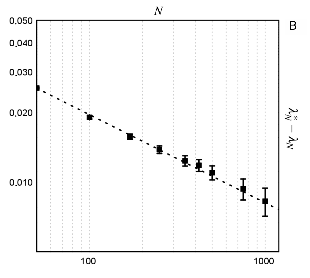
Figure 4: Comparison between the critical ISAW energy from independent PERM simulations with the estimator of Eq. (51) up to $N=1000$ computed with an unbiased algorithm. In figure A, semi-log scale, the black line is the estimator $\lambda_{N}^{*}$ with its error (standard deviation), obtained from an unbiased simulation, while the black dots are values obtained with an independent PERM simulation. Finally, the white squares are the intercepts at $M=0$ from linear fits of Figure 3. B shows the difference $\lambda_{N}^{*}-\lambda_{N}$ between ISAW critical energy and Eq. (51) in log-log scale. The difference is fitted with a power law $K_{0}\,x^{-c}$, with $K_{0}=0.1124\pm 0.0005$ and exponent $c=-0.38\pm 0.01$.

IV Conclusions and Outlooks

Concerning the form of the transition line, it is important to remark that the conjecture in Eq. (51) would open interesting analytic possibilities. In fact, the quantity $\delta_{N}^{*}$ does not depend on $\beta$ and all the averages are taken with respect to the SRW measure. We expect that, apart from messy algebra, the asymptotics of the necessary correlation functions can be computed using the very same techniques developed by Jain and Pruitt to compute the variance of the SRW range Huges ; Jian-Pruitt ; Jiain-Orey ; Dvoretzky-Erdos ; Den Hollander . This would be a nice result, since to the best of our knowledge no exact expression is known or even conjectured for the ISAW critical energy.

Another interesting fact is that the model can be described by a generalized urn model. Since $L\left(\omega_{N}\right)$ can increase only if $M\left(\omega_{N}\right)$ does not, it holds

$$L\left(\omega_{N+1}\right)-L\left(\omega_{N}\right)=2d\cdot\pi\left(\omega_{N+1}\right)\left\{1-\left[M\left(\omega_{N+1}\right)-M\left(\omega_{N}\right)\right]\right\}$$ (52)

where we used the symbol

$$\pi\left(\omega_{N}\right)=\langle M\left(\omega_{N+1}\right)-M\left(\omega_{N}\right)|\omega_{N}\rangle_{0}$$ (53)

to indicate the atmosphere of the chain (see frabalz ). Given the urn kernels

$$\pi_{N}^{\left(k\right)}\left(M,L\right)=\langle I\left(L\left(\omega_{N}\right)-L\left(\omega_{N-1}\right)=k\right)\rangle_{M,L}$$ (54)

for $0\leq k\leq 2d$ we conjecture that

$$\pi^{\left(k\right)}\left(m,\lambda\right)=\lim_{N\rightarrow\infty}\pi_{N}^{\left(k\right)}\left(\left\lfloor mN\right\rfloor,\left\lfloor\lambda N\right\rfloor\right)$$ (55)

exists for all considered $k$, and that it would be possible to extend the urn techniques presented in frabalz ; fra urne to deal with the urn model controlled by the kernels $\pi^{\left(k\right)}\left(m,\lambda\right)$. Notice that for $k=0$ one would have

$$\pi_{N}^{\left(0\right)}\left(M,L\right)=\langle I\left(L\left(\omega_{N}\right)-L\left(\omega_{N-1}\right)=0\right)\rangle_{M,L}=\langle I\left(M\left(\omega_{N}\right)-M\left(\omega_{N-1}\right)=1\right)\rangle_{M,L}$$ (56)

and that by definition must hold

$$1-\pi_{N}^{\left(0\right)}\left(M,L\right)=\sum_{k=1}^{2d}\pi_{N}^{\left(k\right)}\left(M,L\right).$$ (57)

We conclude with one last remark. Due to difficulties in simulating long chains when $m$ is close to $1$ we where unable to directly check the behavior in this region. At first we where tempted to further push the conjecture and guess that in the TL the critical line hits the value $\lambda=0$ at $m=1$, but our PERM estimates seem to exclude this simple ansatz because the observed $\lambda_{N}\left(1\right)$ is always below the value $\lambda_{c}=\lambda_{0}/\left(1-C_{3}\right)\simeq 1.5238$ for which a “linear” critical line can pass through the point $(m_{0},\,\lambda_{0})$, that must lie on the critical line in any case (from SRW theory $\lambda_{0}=6\cdot C_{3}/(1+C_{3})\simeq 1.005$ and $m_{0}=C_{3}\simeq 0.3405$ Douglas ), and then hit the boundary $3\left(1-m\right)$ of the allowed parameter space at $m=1$ exactly.

Then, if the linear behavior of $\ell_{N}\left(m\right)$ can be really extended in the whole $m$ range and $\lambda_{c}<\lambda_{0}/\left(1-C_{3}\right)$ this would imply the existence of a second critical value for the intersection density, ie the $m^{*}=C_{3}\cdot(\lambda_{c}-3)/(\lambda_{c}-\lambda_{0}-3\cdot C_{3})$ at which the crossing between the critical line $\ell_{c}\left(m\right)$ and the boundary $3\left(1-m\right)$ actually happens, and after this value the clustered phase would not be possible anymore except for values of $\lambda$ concentrating on the boundary of the parameter range. For or example, the conjecture would imply that no CG transition can occur for $m<1$ in the $\Omega_{N}\left(\left\lfloor mN\right\rfloor,\left\lfloor\left(1-m\right)N\right\rfloor\right)$ model, where the exceeding nearest neighbor pairs are forbidden. This is likely because in a clustered phase we necessarily have a partial saturation of the nearest neighbor sites of each monomer, and such phase would be extremely unfavored by a small link density.

V Acknowledgments

We would like to thank Giorgio Parisi (Sapienza Univeristà di Roma) and Valerio Paladino (Amadeus IT) for interesting discussions and suggestions. This project has received funding from the European Research Council (ERC) under the European Union’s Horizon 2020 research and innovation programme (grant agreement No [694925]).

References

• (1) P. J. Flory, Principles of Polymer Chemistry (Cornell University Press, 1971).
• (2) I. Nishio, S.-T. Sun, G. Swislow and T. Tanaka, Nature 281, 208–209 (1979).
• (3) K. Minagawa Y. Matsuzawa K. Yoshikawa A. R. Khokhlov and M. Doi, Biopolymers 34, 555-558 (1994).
• (4) P. G. de Gennes, Scaling Concepts in Polymer Physics, Cornell University Press (1979).
• (5) J. des Cloizeaux and G. Jannink, Polymers in solutions: Their Modelling and Structure, Clarendon Press, Oxford (1990).
• (6) A. Y. Grosberg and D. V. Kuznetsov, Macromolecules 25, 1970 (1992).
• (7) P. P. Nidras, J. Phys. A: Math. Gen. 29, 7929 (1996).
• (8) M. C. Tesi, E. J. J. van Rensburgd, E. Orlandini and S. G. Whittington, J. Phys. A: Math. Gen. 29 2451 (1996).
• (9) M. C. Tesi, E. J. J. van Rensburg, E. Orlandini and S. G. Whittington, J. Stat. Phys. 82, 155–181 (1996).
• (10) S. Caracciolo, M. Gherardi, M. Papinutto and A. Pelissetto, J. Phys. A 44, 115004 (2011).
• (11) C.-N. Chen, Y.-H. Hsieh and C.-K. Hu, EPL 104, 20005 (2013).
• (12) N. R. Beaton, A. J. Guttmann and I. Jensen, J. Phys. A: Math. Theo. 53, 165002 (2020).
• (13) C. Domb and G. S. Joyce, J. Phys. C: Solid State Phys. 5, 956 (1972).
• (14) N. Clisby, J. Phys.: Conf. Ser. 921 012012 (2017).
• (15) G. Slade, Proc. R. Soc. A, 475, 20181549 (2019).
• (16) J. F. Douglas and T. Ishinabe, Phys. Rev. E 51, 1791 (1995).
• (17) N. Madras and G. Slade, The Self-Avoiding Walk (Birkhauser, Boston, 1996).
• (18) N. Clisby, Phys. Rev. Lett. 104, 055702 (2010).
• (19) N. Clisby, J. Phys. A: Math. Theor. 34, 5773 (2013).
• (20) S. Franchini, Phys. Rev. E 84, 051104 (2011).
• (21) S. Franchini and R. Balzan, Phys. Rev. E 98, 042502 (2018).
• (22) The Pruned-Enriched Rosenbluth Method (PERM) is a classic stochastic growth algorithm which combines the Rosenbluth-Rosenbluth method with recursive enrichment. One starts by building instances according to a biased distribution, then corrects for this by cloning desired and killing undesired configurations to contain the weights fluctuations, see Grassberger ; Prellberg ; Hsu-Grassberger for reviews and Grassberger for a pseudocode.
• (23) P. Grassberger, Phys. Rev. E 56, 3682 (1997).
• (24) T. Prellberg and J. Krawczyk, Phys. Rev. Lett. 92, 120602 (2004).
• (25) H.-P. Hsu and P. Grassberger, J. Stat. Phys. 144, 597 (2011).
• (26) Although the choice $r=1$ smoothly connects with the SRW we remark that by Eq.(29) the level lines $\ell_{N}\left(m,r\right)$ will eventually converge to the critical line for any fixed $r$.
• (27) See for example the $\Omega_{N}$ $\left(M\right)$ model of frabalz , where the product measure condition is likely to give only approximate results for any $d<\infty$ due to excluded volume effects.
• (28) F. Spitzer, Principles of Random Walk (Springer, New York, 2001).
• (29) B. D. Hughes, Random Walks and Random Enviroments, Vol.1 (Clarendon Press, Oxford, 1995).
• (30) W. Feller, An introduction to Probability Theory and Its Applications, Vol. 1 (Wiley, New York, 1950).
• (31) N. C. Jain and W. E. Pruitt, J. Analyse Math. 24, 369 (1971).
• (32) N. C. Jain, S. Orey, Isr. J. Math. 6, 373 (1968).
• (33) A. Dvoretzky and P. Erdos, Proc. 2nd Berkley Symp. on Prob. and Stat., 353 (1951).
• (34) S. Franchini, Stoc. Proc. Appl. 127 (2017).
• (35) F. Den Hollander, J. Stat. Phys. 37 (1984) 331-367.
• (36) D.C. Brydges and G. Slade, J. Stat. Phys. 159 (2015) 421-667.