Direct Measurement of the Solar-Wind Taylor Microscale using MMS Turbulence Campaign Data

Abstract

Using the novel Magnetospheric Multiscale (MMS) mission data accumulated during the 2019 MMS Solar Wind Turbulence Campaign, we calculate the Taylor microscale $(\lambda_{\mathrm{T}})$ of the turbulent magnetic field in the solar wind. The Taylor microscale represents the onset of dissipative processes in classical turbulence theory. An accurate estimation of Taylor scale from spacecraft data is, however, usually difficult due to low time cadence, the effect of time decorrelation, and other factors. Previous reports were based either entirely on the Taylor frozen-in approximation, which conflates time dependence, or that were obtained using multiple datasets, which introduces sample-to-sample variation of plasma parameters, or where inter-spacecraft distance were larger than the present study. The unique configuration of linear formation with logarithmic spacing of the 4 MMS spacecraft, during the campaign, enables a direct evaluation of the $\lambda_{\mathrm{T}}$ from a single dataset, independent of the Taylor frozen-in approximation. A value of $\lambda_{\mathrm{T}}\approx 7000\,\mathrm{km}$ is obtained, which is about 3 times larger than the previous estimates.

1 Introduction: Turbulence Scales

Turbulence is a multi-scale phenomena. The turbulent solar wind possesses structures and processes with broad range of length scales (Verscharen et al., 2019). The different characteristic length scales enter into the dynamics in various ways. For example, the correlation scale represents the sizes of the most energetic eddies (Smith et al., 2001). The mean-free path between collisions determine the collisionality of the plasma. Proton kinetic physics dominates near the proton inertial length and gyro-radius (Leamon et al., 1998); similarly electron physics becomes important at the electron inertial length and gyro-radius (Alexandrova et al., 2012). These different characteristic scales can provide useful information regarding the propagation of energetic particles, such as cosmic rays in the solar wind (Jokipii, 1973).

Of these various scales there are several related directly to fundamental turbulence properties, and understanding these in various space and astrophysical venues contributes in the understanding of physical effects ranging from reconnection to particle heating and scattering. For an initial orientation, We can appeal to analogies with hydrodynamics, to outline relationships that exist among these scales in classical turbulence. Accordingly, we use as a reference point the case in which the dissipation is controlled by a simple scalar kinematic viscosity $\nu$. We may begin with the scale at which the bulk of turbulence energy resides, or is injected; we call this the energy-containing scale $\lambda_{\mathrm{c}}$. For a turbulence amplitude $Z$, with units of speed, one finds immediately a nonlinear time scale, or the eddy turnover time $\tau_{\mathrm{nl}}=\lambda_{\mathrm{c}}/Z$. Smaller scale structures will have faster time scales that depend on their characteristics speeds. Using Kolmogorov’s famous similarity hypothesis as a guide (Kolmogorov, 1941), we may estimate the speed of structures at smaller scales $\ell$ to be $Z_{\ell}\sim\epsilon^{1/3}\ell^{1/3}=\tau_{\mathrm{nl}}(\ell/L)^{2/3}$, where we also use the de Kármán & Howarth (1938) estimate of the decay rate $\epsilon\sim Z^{3}/\lambda_{\mathrm{c}}$. probing at still smaller scales, very much smaller than $\lambda_{\mathrm{c}}$, eventually dissipative processes of viscous origin become important. As a first approximation one may estimate the time scale for dissipation of a structure (e.g., a vortex) at scale $\ell$ to be $\tau_{\mathrm{diss}}=\ell^{2}/\nu$, using standard viscous dissipation as a model. A reasonable way to estimate the characteristic scale at which dissipation becomes dominant is to ask when the eddy or structure at scale $\ell$ become critically damped. This occurs when the intrinsic nonlinear time balances the local-in-scale dissipative time. For this, we solve $\tau_{\mathrm{nl}}(\eta)=\tau_{\mathrm{diss}}(\eta)$ finding $\eta=\lambda_{\mathrm{c}}(\nu/Z\lambda_{\mathrm{c}})^{3/4}=\lambda_{\mathrm{c}}Re^{-3/4}$. The scale $\eta$ is often called the Kolmogorov dissipation scale, and we recognize standard definition of the large scale Reynolds number $Re\equiv{Z\lambda_{\mathrm{c}}/\nu}$. Note that if the critically damped scale is known or estimated, as it might be in a plasma identified with ion inertial scale for example, then the effective Reynolds number may be defined as $R_{\mathrm{eff}}=(\lambda_{\mathrm{c}}/\eta)^{4/3}$, or $R_{\mathrm{eff}}=(\lambda_{\mathrm{c}}/d_{\mathrm{i}})^{4/3}$ if dissipation is presumed to become dominant over nonlinear effects at scales comparable to the ion inertial length $d_{i}$.

Yet another scale, generally intermediate to $\lambda_{\mathrm{c}}$ and $\eta$ may be defined by equating the large scale eddy turnover time to the scale-dependent dissipative time. Thus, $\tau_{\mathrm{nl}}=\tau_{\mathrm{diss}}(\ell)$ is solved by a particular value $\ell=\lambda_{\mathrm{T}}$. This length scale is the Taylor microscale, the subject of the present paper. The first of its several equivalent definitions highlights a particular physical property, namely that it is critically damped at the large scale nonlinear time. Before turning to its evaluation in the MMS Turbulence Campaign, we introduce and discuss several additional properties of the Taylor scale $\lambda_{\mathrm{T}}$.

2 Taylor Microscale

Like the majority of concepts in plasma turbulence, the Taylor scale is also borrowed from hydrodynamic turbulence research. The Taylor scale can be viewed as the measure of curvature of the autocorrelation function $\left(R(\mathbf{r})=\langle\mathbf{F}(\mathbf{x})\cdot\mathbf{F}(\mathbf{x}+\mathbf{r})\rangle\right)$ at the origin; for isotropy,

$$\lambda_{\mathrm{T}}^{2}=\frac{R(0)}{R^{\prime\prime}(0)},$$ (1)

where $\mathbf{F}$ is the fluctuating field of interest, e.g., velocity field $(\mathbf{v})$ in hydrodynamic turbulence, or magnetic field $(\mathbf{b})$ in magnetohydrodynamic (MHD) and plasma turbulence. Here, we consider only the magnetic field fluctuations. For small lags $r$, using $R(\mathbf{r})=R(-\mathbf{r})$ , a requirement of statistical homogeneity, the autocorrelation function near the origin can be Taylor expanded, assuming isotropy, as

$$R(r)=1-\frac{r^{2}}{2\,\lambda_{\mathrm{T}}^{2}}+\cdots,$$ (2)

Another physically revealing way to view the Taylor microscale is obtained by noting that for viscous-like $\nu$ dissipation in an incompressible medium, the Taylor scale is also related to dissipation, in that

$$\frac{\mathrm{d}\langle|\mathbf{b}|^{2}\rangle}{\mathrm{d}t}=\nu\langle|\nabla\times{\bf b}|^{2}\rangle=\nu\frac{\langle|\mathbf{b}|^{2}\rangle}{\lambda_{\mathrm{T}}^{2}}.$$ (3)

In this sense, the Taylor scale is the “equivalent dissipation scale,” so that, at any instant of time, the dissipation rate is the same if all the energy were at the Taylor scale. This is, in fact, the physical basis upon which Taylor  (Taylor, 1935) first formulated the idea of this particular length scale. Some older turbulence texts (Hinze, 1975) refer to the Taylor scale as “the dissipation scale,” although later Kolomogrov (Kolmogorov, 1941) introduced the similarity variable $(\eta)$, now known as the Kolmogorov length scale, to denote the scale at which eddies become critically damped. Notionally, the Taylor microscale represents the largest eddies in the dissipation range, or equivalently, the smallest eddies in the inertial range. The interpretation, of course, may not be so straightforward in plasma turbulence. However, one may draw some conclusions by analogy with hydrodynamics.

Keeping this parallel in mind, we recall that, indeed, space plasma observations show that the transition of Kolmogorov -5/3 spectra to a steeper slope occur at somewhat larger scales than ion-inertial scale or proton gyro radius (Leamon et al., 2000). In classical hydrodynamic turbulence, the Taylor scale is greater than the Kolmogorov length scale $(\eta)$. Therefore, if one treats the ion-inertial length or the proton gyro radius as equivalent to the classical-turbulence Kolmogorov scale, where dissipative (or kinetic) processes become dominant, the Taylor scale provides a natural descriptor of the slight steepening of spectra, and the onset of dissipation, prior to dissipation becoming dominant at still smaller scales. This also fits well with the idea, from reconnection studies, that intense kinetic activity in current sheets is initiated at some multiple of the ion scales (Shay et al., 1998)

3 Limitations

The computation of Taylor microscale is, however, challenging in spacecraft data due to low temporal cadence, and other factors, as discussed in the following. The primary hindrance in accurate estimation of Taylor microscale, using spacecraft data, comes from the approximation due to Taylor’s frozen-in hypothesis (Taylor, 1938). In-situ spacecraft data are usually collected in the form of time signals at the spacecraft location. However, usually in the solar wind, the Alfvén speed is much smaller than the flow speed, so that one may assume, to a good approximation, that the plasma is frozen-in to the flow (Jokipii, 1973). Therefore, as the plasma convects past the spacecraft, the collected time series data can be essentially interpreted as an one-dimensional “cut” through the three-dimensional plasma. This is the interplanetary spacecraft version of the Taylor’s frozen-in wind-tunnel approximation. In spite of the widespread utility of this approach, it is apparent that, when available, the correct way to probe spatial structures is through simultaneous multi-point observations (Matthaeus et al., 2019). Moreover, the Taylor approximation is only well-justified for inertial-scale and somewhat larger fluctuations, as high frequency kinetic activity at sub-proton scales might introduce substantial inaccuracy (Roberts et al., 2020).

However, the evaluation of $\lambda_{\mathrm{T}}$, requires measurement of the curvature of the correlation function near the origin, precisely demanding such information regarding small spatial range fluctuations. But simultaneous multi-point data, especially at small separation, have generally not been available. Even when multi-point measurements have been obtained, those intervals are typically not very long (e.g., Roberts et al., 2015; Chasapis et al., 2017). For statistical studies of turbulence in the solar wind, continuous intervals of duration of at least a few hours, corresponding to at least a few spacecraft-frame correlation times, are desirable (Isaacs et al., 2015). Consequently, previous studies were forced to perform analyses compiled from a number of different intervals. At that point, additional uncertainty is introduced by variation of plasma conditions from interval-to-interval. The first MMS mini campaign, named the MMS Solar-Wind Turbulence Campaign, explicitly overcomes these limitations, as discussed in the next section. However, we note that the data studied are also limited in that there is one sampling direction i.e., all spacecraft are in a line. Although four-point measurements provide many advantages, this and other related limitations are intrinsic to four-point measurements.

4 MMS Solar-Wind Turbulence Campaign

The Magnetospheric Multiscale (MMS) mission, was launched in 2015 with the primary goal of studying magnetic reconnection — a process responsible for releasing magnetic energy into flows and internal energy. The four MMS spacecraft are equipped with state-of-the-art instruments with unprecedented resolution. During February 2019, the MMS apogee was raised to $\sim 27\,\mathrm{R_{E}}$ on Earth’s dayside of the magnetosphere and outside the ion foreshock region. This orbit allowed the spacecraft to sample the pristine solar wind, outside the Earth’s magnetosheath and far from the bow shock, for extended periods of time (see Fig. 1).

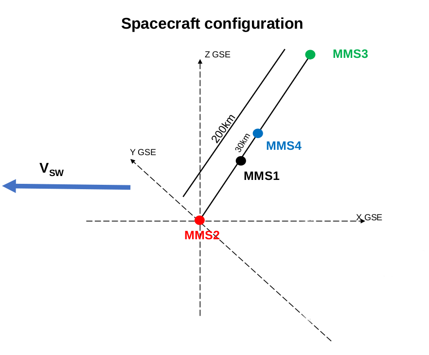
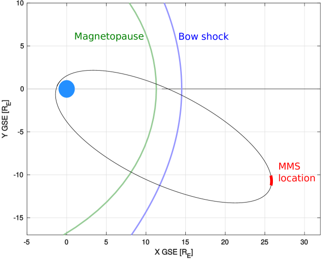
Figure 1: Top: Configuration of the 4 MMS spacecraft and the flow speed direction during the MMS turbulence campaign. Bottom: Location of the MMS, along with the nominal magnetopause and bow-shock locations. The Geocentric Solar Ecliptic (GSE) (Franz & Harper, 2002) coordinate system is used, in which the XY-plane is defined by the Earth mean ecliptic and the +X-axis is defined by the Earth-Sun vector.

During the first mini campaign, the four MMS spacecraft were arranged in a “string of pearls” or “beads on string” formation instead of the usual tetrahedral formation. With the spacecraft baseline almost perpendicular to the solar wind flow, the spacecraft were separated by logarithmic distances ranging from 25 to 200 km, and the baseline separations remain unchanged within $10\%$. This configuration allows direct investigation of the scale-dependent nature of the solar wind structures near proton scales. Laboratory experiments have utilized such formations (Cartagena-Sanchez et al., 2019), but this kind of data are novel in observations. This work is the first of several studies undertaken to take advantage of this unique configuration (see also Chasapis et al. (2020)). Although not relevant for this study, the spacecraft spin-axis were tilted about 15^∘ to obtain improved electric field measurements in the solar wind. A schematic configuration of the four MMS spacecraft in the solar wind, during the Turbulence Campaign, is provided in the top panel of Fig. 1. The orbital context plot showing MMS location relative to the nominal magnetopause (Shue et al., 1998) and bow shock (Farris & Russell, 1994), is illustrated in the bottom panel of Fig. 1.

5 MMS Data

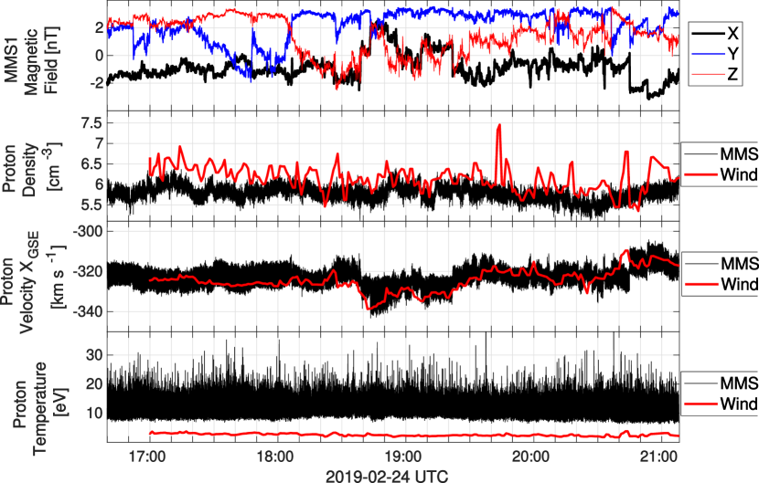
Figure 2: Time series of solar wind observations from 16:39:00 - 21:41:00 UTC on 24 Feb 2019. Top panel: GSE components ofthe MMS1/FGM magnetic field, second panel: Proton number density measured by MMS1 and Wind, third panel: X component of the proton velocity, in GSE coordinate system, measured by MMS1 and Wind, bottom panel: Proton temperature measured by MMS1 and Wind.

Table 1: Parameters for MMS interval on 24 February 2019, from 16:00 to 21:00 UTC (5 hours). Quantities with an asterisks $(^{*})$ have been estimated using Wind data, and for those, the MMS estimates are given in parenthesis.

Solar-wind speed	$V_{\mathrm{SW}}=$ 322 km s-1
Correlation Length	$\lambda_{\mathrm{c}}=3.2\times 10^{5}$ km
Ion inertial length	$d_{\mathrm{i}}=$ 91 km
Ion gyroradius	$\rho_{\mathrm{i}}=$ 64∗ (150) km
Electron inertial length	$d_{\mathrm{e}}=$ 2.3 km
Debye length	$\lambda_{D}=$ 10 m
Proton beta	$\beta_{\mathrm{i}}=$ 0.5∗ (2.5)
Magnetic field	$B_{0}=|\langle\mathbf{B}\rangle|=$ 3.4 nT
Magnetic-field fluctuation	$B_{\mathrm{rms}}/B_{0}=$ 0.72
Proton density	$\langle N_{\mathrm{i}}\rangle=$ 6.2 cm-3
Proton temperature	$\langle T_{\mathrm{i}}\rangle=$ 2.5∗ (12.4) eV

During the three-week long mini campaign, a number of useful solar wind and foreshock intervals were selected. The longest of the selected pristine solar wind intervals, a continuous interval of five hours of burst-mode data, on 24 February 2019, from 16:39:00 to 21:41:00 UTC, is analyzed in this paper. No signature of reflected ions from the bow shock is found. For this interval, we did not detect any high-frequency waves characteristic of the foreshock. We note, however, that the other 5-hour interval (17 February 2019, from 11:24:00 to 16:24:00 UTC) chosen as a part of the turbulence campaign, has foreshock signatures, and consequently that interval was not considered for this analysis.

To evaluate the magnetic field Taylor microscale from two-spacecraft correlation data, We employ data from the Fluxgate Magnetometer (FGM) aboard each each of the four MMS spacecraft(Russell et al., 2016). The top panel of Fig. 2 shows the three Cartesian components of magnetic field in the GSE coordinate system (Franz & Harper, 2002), recorded in this period by the FGM onboard MMS1. It is apparent that this interval is rich in structures, including numerous current sheets, flux tubes, and broad band random fluctuations - taken together these represent a fairly typical sample of solar wind turbulence (Bruno & Carbone, 2005).

The Fast Plasma Investigation (FPI) (Pollock et al., 2016) instrument measures proton and electron distribution functions and moments every 150ms and 30ms, respectively. Due to the limitations of the FPI instruments in the solar wind (Bandyopadhyay et al., 2018a), some systematic uncertainties remain in the moments, and more so in the higher-order moments. Therefore, we cross-check the proton moments in the selected interval with Wind (Ogilvie et al., 1995; Lepping et al., 1995) data, time-shifted to the bow-shock nose. The MMS and Wind estimates of proton density, velocity (X_GSE component), and temperature are shown in the bottom three panels in Fig. 2. The density and velocity are in adequately close agreement, but significant discrepancies exist in the proton temperature values. The FPI estimates of temperature are significantly greater than the Wind values. Given the known limitations of FPI in the solar wind, we use the Wind measurements of temperature to evaluate proton beta and other relevant parameters. The average values of the plasma parameters are reported in Table 1.

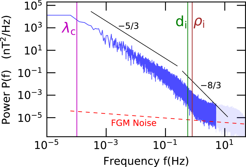
Figure 3: Spectral power density of magnetic field measured by MMS1. Kolmogorov scaling $\sim f^{-5/3}$ is shown for reference. The vertical lines represent the correlation length $(k\lambda_{\mathrm{c}}=1)$, the ion-inertial length $(kd_{\mathrm{i}}=1)$, and the ion gyro-radius $(k\rho_{\mathrm{i}}=1)$, with wavenumber $k\simeq(2\pi f)/|\langle\mathbf{V}\rangle|$. The part of the spectrum where the signal-to-noise ratio decreases below $\sim 5$, is grey-shaded, to indicate that this region is noise dominated. Note that the flattening in the high-frequency range ($f\gtrsim 1$ Hz) is due to noise and not physical (see text).

Fig. 3 shows spacecraft-frame frequency spectrum of the magnetic field during this period. A clear Kolmogorov scaling $(\sim f^{-5/3})$ can be seen at scales smaller than the correlation length, $\lambda_{\mathrm{c}}$ (inferred from the Taylor hypothesis). A break in spectral slope from $\sim f^{-5/3}$ to $\sim f^{-8/3}$ is observed near (inferred) kinetic scales ($d_{\mathrm{i}}$ or $\rho_{\mathrm{i}}$). Often these scales are associated with the dissipation scale $(\lambda_{\mathrm{diss}})$ in collisionless plasmas, equivalent to Kolmogorov scale $(\eta)$ in classical turbulence. Kinetic dissipative processes, such as wave damping, are effective in these small plasma kinetic scales. For example, Leamon et al. (2000) and Wang et al. (2018) argued that the ion inertial scale controls the spectral break and onset of strong dissipation, while Bruno & Trenchi (2014) suggested the break frequency is associated with the resonance condition for parallel propagating Alfvén wave. Another possibility is that the largest of the proton kinetic scales terminates the inertial range and controls the spectral break(Chen et al., 2014). The flattening near $f\gtrsim 1$ Hz is very likely to be noise dominated, since, for example, this behavior is not seen in Cluster search coil observations (e.g., Alexandrova et al., 2009, 2012; Roberts et al., 2017).

6 Taylor Microscale: Results

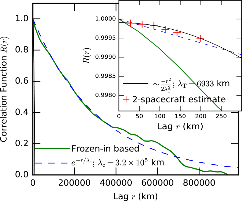
Figure 4: Magnetic-field correlation function based on frozen-in approximation (green, solid line) and obtained from two-spacecraft evaluation (red, cross symbols). An exponential fit (blue, dashed line) to the single-spacecraft measurement is used to obtain the correlation length. A quadratic fit (black, thin line) to the multi-spacecraft points estimates the Taylor scale. The inset plots part of the correlation function enlarged near the origin to clearly show the multi-spacecraft points and the parabolic fit.

To estimate the Taylor scale from this interval, we recall the approximation near the origin:

$$R(r)\approx 1-\frac{r^{2}}{2\,\lambda_{\mathrm{T}}^{2}},$$ (4)

where the higher-order terms are neglected. Therefore, one may obtain the Taylor microscale by fitting the autocorrelation function $R(r)$ to a parabolic curve at the origin. Clearly, the quadratic approximation holds better as one asymptotically approaches smaller values of $r$. Previous multi-spacecraft estimates (Matthaeus et al., 2005) were evaluated with the Cluster spacecraft, with separations in the range 150 km $\leq r\leq$ 270 km. Here, we extend that analysis by approaching the origin closer by about an order of magnitude, with 25 km $\leq r\leq$ 200 km. Appendix A provides an estimate of the accuracy of the correlation measurements. As shown in Fig. 4, we extract an estimate of $\lambda_{\mathrm{T}}$ by fitting the the six available two-point correlation function to a parabolic curve. The resulting value of the Taylor scale is $\lambda_{\mathrm{T}}=6933$km. For comparison, we also show the single-spacecraft, frozen-in hypothesis based evaluation of the correlation function. Evidently, the single-spacecraft estimate decays much rapidly closer to the origin, presumably due to time decorrelation of the solar wind fluctuations in those scales (Matthaeus et al., 2010). At large lags, however, the frozen-in based correlation function exhibits approximately exponential decay and provides a satisfactory estimate of the correlation length, about $320,000$km, consistent with previous reports (Isaacs et al., 2015). Note that the exponential passes close to the multi-spacecraft points (see inset) near the origin; however, the exponential cannot be employed to determined $\lambda_{\mathrm{T}}$ since the curvature at the origin is undefined.

Solar wind viscosity– An accurate estimation of the Taylor scale also permits an evaluation of an effective viscosity (or, turbulent viscosity/resisivity) of the solar wind, according to the expression,

$$\nu=\frac{\epsilon}{2E}\lambda_{T}^{2},$$ (5)

where $\epsilon$ is the cascade rate $\approx 1000\,\mathrm{J\,kg\,s^{-1}}$ and $E$ is the fluctuation energy per unit mass. The cascade rate can be obtained, for example, from the third order law or other estimates, see e.g., Verma et al. (1995); Sorriso-Valvo et al. (2007); MacBride et al. (2008); Bandyopadhyay et al. (2018b). Putting in the rest of the values: $\lambda_{\mathrm{T}}=6933$ km and $2E=\langle|\mathbf{b}|^{2}\rangle=324\,\mathrm{km}^{2}\,\mathrm{s}^{-2}$, we obtain $\nu\approx 150\,\mathrm{km}^{2}\,\mathrm{s}^{-1}$. This value is considerably larger than the one obtained using Braginskii (Braginskii, 1965) formalism, which is based on simple particle-particle collision (Montgomery, 1983). Our result also provides improvement on earlier indirect estimates, based on turbulence-cascade phenomenology (Coleman, 1968; Verma, 1996).

7 Discussion and Conclusions

In this paper, MMS data accumulated during the turbulence campaign have been used to evaluate the Taylor microscale of magnetic field fluctuations using a multi-spacecraft technique, and taking advantage of a unique beads-on-a-string flight formation. The previous estimate by Matthaeus et al. (2005), using Cluster data, is $\lambda_{\mathrm{T}}=2478$ km, which is about 3 times smaller than the present evaluation. The deviation is possibly due to the relatively larger spacecraft separation used in the Cluster data set, comparatively shorter intervals, and mixing of different solar wind intervals. It is also possible that this level of variability is intrinsic to the solar wind for a variety of reasons including $1/f$ noise, stream structure (Matthaeus & Goldstein, 1986). Another possibility is that the differences may be attributable to the differences in the formation of the Cluster and MMS spacecraft. The Cluster spacecraft pair baselines are in a tetrahedron, introducing anisotropy effects, which are not present in the MMS linear formation analyzed here. These limitations are inherent to four-point measurements, and can be overcome by large constellations of simultaneous, in-situ measurements (Matthaeus et al., 2019; Klein et al., 2019; TenBarge et al., 2019).

We note here that the two-spacecraft data points cover a very small range, in contrast with the frozen-in based correlation function (compare the inset in Fig. 4 to the main plot). We, however, do not expect any weakness in the analysis due to this point. The estimation of correlation length by an exponential approximation is only valid at long lag, while the quadratic approximation to the expansion of the correlation function is expected to hold only near the origin. Therefore, the small coverage of scale is not expected to hinder the Taylor-scale estimation.

We find that the break frequency, in the magnetic-field spectrum, is situated between the Taylor scale $(\lambda_{\mathrm{T}})$ and dissipative scales $(d_{\mathrm{i}},\rho_{\mathrm{i}})$. Wang et al. (2018), showed that for $\beta\sim 1$ plasma, the spectral break frequency is better associated with $d_{\mathrm{i}}$ than $\rho_{\mathrm{i}}$, and it is insensitive to $\beta$-values. In general, $\lambda_{\mathrm{T}}/\lambda_{\mathrm{diss}}>1$ in hydrodynamic turbulence, and the separation increases with Reynolds number. Although the dissipation mechanism in the collsiionless solar wind is not due to a viscous closure, we note here that if one associates the ion-inertial length $d_{\mathrm{i}}$ or ion gyro-radius $\rho_{\mathrm{i}}$ with the dissipation scale, then we find that $\lambda_{\mathrm{T}}/\lambda_{\mathrm{diss}}\approx 70$. The relationship of Taylor scale to ion kinetic scales in the solar wind however, appears to be much more variable than it is in hydrodynamics, and in particular the relationship has been found to depend on the turbulence cascade rate (Matthaeus et al., 2008).

The present paper is a step in a broad progression of interplanetary measurements of fundamental plasma turbulence properties. The 1980 NASA Plasma Turbulence Explorer Panel emphasized the need for simultaneous multi-point measurements, in particular, plasma and magnetic field measurements, to make progress in this area (Montgomery & et al., 1980). More recently, the space plasma community has witnessed growing interest in understanding the multi-scale nature of turbulence processes in space, using multi-point measurements in observations (Matthaeus et al., 2019; Klein et al., 2019) as well as laboratory experiments (Schaffner et al., 2014; Schaffner & Brown, 2015), especially with regard to the physics of dissipation and heating mechanisms. The MMS turbulence campaign provides the first opportunity to capture multi-scale processes near the proton scales with a single data interval. Therefore, the results presented in this paper will be useful for future and proposed multi-spacecraft missions (Vaivads et al., 2016; Bookbinder et al., 2018; Plice et al., 2019; Verscharen & Wicks, 2019; Wicks & Verscharen, 2019).

The 2019 Solar Wind turbulence campaign is the first of the many MMS mini-campaigns that are planned to be held in the second extended mission phase. The results presented in this paper will serve as a demonstration of the MMS instrumental capabilities, working outside their original region of interest. Exploring the potential advantages of different MMS formations will allow better understanding of MMS range of capabilities, which will open the door to other scientific campaigns.

Appendix A Measure of Confidence in the two-spacecraft analyses

As can be seen in Fig. 4, the signals between spacecraft are strongly correlated; however, the differences are very small between them. The very small variation in the 2-spacecraft correlations, between $1$ and $0.9995$, calls for further analyses of its accuracy. Here, we provide an error estimate to check the quality of the measurements.

Recall the definition of correlation function for magnetic-field fluctuations $\mathbf{b}$,

$$R(\mathbf{r})=\langle\mathbf{b}(\mathbf{x})\cdot\mathbf{b}(\mathbf{x}+\mathbf{r})\rangle.$$ (A1)

Keeping in mind that the uncertainty in FGM magnetic field measurements are less than $\delta b=0.1$ nT (Russell et al., 2016), and that the average magnetic field is about $b\sim 2$ nT, the fractional error in the individual sample points of the correlation function, $\mathbf{b}(\mathbf{x})\cdot\mathbf{b}(\mathbf{x}+\mathbf{r})$, is less than $2\delta b/b\sim 0.1$. Further, averaging over all the data points reduces the statistical error by $\sim 1/\sqrt{n}$, where $n$ is the number of data points (The error in the mean estimate would be even smaller by another factor of $1/\sqrt{n}$). So we estimate the error in the 2-spacecraft $R(r)$ as $\delta R/R\sim 10^{-7}$. Therefore, even by a very conservative estimate, the 2-spacecraft values are reliable up to $6$ decimal points. Finally, the root-mean-square of two-spacecraft magnetic-field increments, for the smallest separation, is about 5 times larger than the noise level at the scale of spacecraft separation (also see Chhiber et al., 2018), so that we expect that the 2-spacecraft signals are larger than the instrumental noise. These tests indicate that the two-spacecraft analyses are indeed reliable.

References

- Alexandrova et al. (2012) Alexandrova, O., Lacombe, C., Mangeney, A., Grappin, R., & Maksimovic, M. 2012, The Astrophysical Journal, 760, 121, doi: https://doi.org/10.1088/0004-637X/760/2/121
- Alexandrova et al. (2009) Alexandrova, O., Saur, J., Lacombe, C., et al. 2009, Phys. Rev. Lett., 103, 165003, doi: 10.1103/PhysRevLett.103.165003
- Bandyopadhyay et al. (2018a) Bandyopadhyay, R., Chasapis, A., Chhiber, R., et al. 2018a, The Astrophysical Journal, 866, 81, doi: https://doi.org/10.3847/1538-4357/aade93
- Bandyopadhyay et al. (2018b) —. 2018b, The Astrophysical Journal, 866, 106, doi: https://doi.org/10.3847/1538-4357/aade04
- Bookbinder et al. (2018) Bookbinder, J., Spence, H. E., Kasper, J. C., Klein, K. G., & Zank, G. P. 2018, in AGU Fall Meeting Abstracts, Vol. 2018, SH33D–3673
- Braginskii (1965) Braginskii, S. I. 1965, Rev. Plasma Phys., 1, 205
- Bruno & Carbone (2005) Bruno, R., & Carbone, V. 2005, Living Reviews in Solar Physics, 2, 4, doi: 10.12942/lrsp-2005-4
- Bruno & Trenchi (2014) Bruno, R., & Trenchi, L. 2014, The Astrophysical Journal, 787, L24, doi: 10.1088/2041-8205/787/2/l24
- Cartagena-Sanchez et al. (2019) Cartagena-Sanchez, C. A., Schaffner, D. A., Slanksi, A., et al. 2019, in APS Meeting Abstracts, Vol. 2019, APS Division of Plasma Physics Meeting Abstracts, UP10.113
- Chasapis et al. (2017) Chasapis, A., Matthaeus, W. H., Parashar, T. N., et al. 2017, Astrophys. J., 836, 247, doi: 10.3847/1538-4357/836/2/247
- Chasapis et al. (2020) Chasapis, A., Matthaeus, W. H., Bandyopadhyay, R., et al. 2020, In Preparation
- Chen et al. (2014) Chen, C. H. K., Leung, L., Boldyrev, S., Maruca, B. A., & Bale, S. D. 2014, Geophys. Res. Lett., 41, 8081, doi: 10.1002/2014GL062009
- Chhiber et al. (2018) Chhiber, R., Chasapis, A., Bandyopadhyay, R., et al. 2018, Journal of Geophysical Research: Space Physics, 123, 9941, doi: 10.1029/2018JA025768
- Coleman (1968) Coleman, P. J. 1968, The Astrophysical Journal, 153, 371, doi: 10.1086/149674
- de Kármán & Howarth (1938) de Kármán, T., & Howarth, L. 1938, Proc. Roy. Soc. London Ser. A, 164, 192, doi: 10.1098/rspa.1938.0013
- Farris & Russell (1994) Farris, M. H., & Russell, C. T. 1994, Journal of Geophysical Research: Space Physics, 99, 17681, doi: 10.1029/94JA01020
- Franz & Harper (2002) Franz, M., & Harper, D. 2002, Planetary and Space Science, 50, 217, doi: 10.1016/S0032-0633(01)00119-2
- Hinze (1975) Hinze, J. O. 1975, Turbulence (New York: McGraw Hill)
- Isaacs et al. (2015) Isaacs, J. J., Tessein, J. A., & Matthaeus, W. H. 2015, Journal of Geophysical Research: Space Physics, 120, 868, doi: 10.1002/2014JA020661
- Jokipii (1973) Jokipii, J. R. 1973, Annual Review of Astronomy and Astrophysics, 11, 1, doi: 10.1146/annurev.aa.11.090173.000245
- Klein et al. (2019) Klein, K. G., Alexandrova, O., Bookbinder, J., et al. 2019, arXiv e-prints, arXiv:1903.05740. https://arxiv.org/abs/1903.05740
- Kolmogorov (1941) Kolmogorov, A. N. 1941, Dokl. Akad. Nauk SSSR, 30, 301, doi: 10.1098/rspa.1991.0075
- Leamon et al. (2000) Leamon, R. J., Matthaeus, W. H., Smith, C. W., et al. 2000, ApJ, 537, 1054, doi: 10.1086/309059
- Leamon et al. (1998) Leamon, R. J., Smith, C. W., Ness, N. F., Matthaeus, W. H., & Wong, H. K. 1998, Journal of Geophysical Research: Space Physics, 103, 4775, doi: 10.1029/97JA03394
- Lepping et al. (1995) Lepping, R. P., Acũna, M. H., Burlaga, L. F., et al. 1995, Space Science Reviews, 71, 207, doi: 10.1007/BF00751330
- MacBride et al. (2008) MacBride, B. T., Smith, C. W., & Forman, M. A. 2008, Astrophys. J., 679, 1644, doi: 10.1086/529575
- Matthaeus et al. (2010) Matthaeus, W. H., Dasso, S., Weygand, J. M., Kivelson, M. G., & Osman, K. T. 2010, Astrophys. J. Lett., 721, L10, doi: 10.1088/2041-8205/721/1/L10
- Matthaeus et al. (2005) Matthaeus, W. H., Dasso, S., Weygand, J. M., et al. 2005, Phys. Rev. Lett., 95, 231101, doi: 10.1103/PhysRevLett.95.231101
- Matthaeus & Goldstein (1986) Matthaeus, W. H., & Goldstein, M. L. 1986, Phys. Rev. Lett., 57, 495, doi: 10.1103/PhysRevLett.57.495
- Matthaeus et al. (2008) Matthaeus, W. H., Weygand, J. M., Chuychai, P., et al. 2008, Astrophysial Journal, 678, L141, doi: 10.1086/588525
- Matthaeus et al. (2019) Matthaeus, W. H., Bandyopadhyay, R., Brown, M. R., et al. 2019, arXiv e-prints, arXiv:1903.06890. https://arxiv.org/abs/1903.06890
- Montgomery (1983) Montgomery, D. 1983, in NASA Conference Publication, Vol. 228, NASA Conference Publication, 0.107. https://ui.adsabs.harvard.edu/abs/1983NASCP.2280.107M
- Montgomery & et al. (1980) Montgomery, D., & et al. 1980, Report of the NASA Plasma Turbulence Explorer Study Group, Vol. 715-78 (NASA, Jet Propulsion Laboratory, Pasadena, CA)
- Ogilvie et al. (1995) Ogilvie, K. W., Chornay, D. J., Fritzenreiter, R. J., et al. 1995, Space Science Reviews, 71, 55, doi: 10.1007/BF00751326
- Plice et al. (2019) Plice, L., Dono Perez, A., & West, S. 2019. https://ntrs.nasa.gov/search.jsp?R=20190029108
- Pollock et al. (2016) Pollock, C., Moore, T., Jacques, A., et al. 2016, Space Science Reviews, 199, 331, doi: 10.1007/s11214-016-0245-4
- Roberts et al. (2017) Roberts, O. W., Alexandrova, O., Kajdic, P., et al. 2017, The Astrophysical Journal, 850, 120, doi: https://doi.org/10.3847/1538-4357/aa93e5
- Roberts et al. (2015) Roberts, O. W., Li, X., & Jeska, L. 2015, The Astrophysical Journal, 802, 2, doi: 10.1088/0004-637x/802/1/2
- Roberts et al. (2020) Roberts, O. W., Nakamura, R., Narita, Y., et al. 2020, EGU General Assembly 2020, doi: https://doi.org/10.5194/egusphere-egu2020-6815
- Russell et al. (2016) Russell, C. T., Anderson, B. J., Baumjohann, W., et al. 2016, Space Science Reviews, 199, 189, doi: 10.1007/s11214-014-0057-3
- Schaffner & Brown (2015) Schaffner, D. A., & Brown, M. R. 2015, The Astrophysical Journal, 811, 61, doi: 10.1088/0004-637X/811/1/61
- Schaffner et al. (2014) Schaffner, D. A., Brown, M. R., & Lukin, V. S. 2014, The Astrophysical Journal, 790, 126, doi: 10.1088/0004-637x/790/2/126
- Shay et al. (1998) Shay, M. A., Drake, J. F., Denton, R. E., & Biskamp, D. 1998, Journal of Geophysical Research: Space Physics, 103, 9165
- Shue et al. (1998) Shue, J.-H., Song, P., Russell, C. T., et al. 1998, Journal of Geophysical Research: Space Physics, 103, 17691, doi: 10.1029/98JA01103
- Smith et al. (2001) Smith, C. W., Matthaeus, W. H., Zank, G. P., et al. 2001, Journal of Geophysical Research: Space Physics, 106, 8253, doi: 10.1029/2000JA000366
- Sorriso-Valvo et al. (2007) Sorriso-Valvo, L., Marino, R., Carbone, V., et al. 2007, Phys. Rev. Lett., 99, 115001, doi: 10.1103/PhysRevLett.99.115001
- Taylor (1935) Taylor, G. I. 1935, Proc. R. Soc. London Ser. A, 151, 421, doi: 10.1098/rspa.1935.0158
- Taylor (1938) —. 1938, Proceedings of the Royal Society of London Series A, 164, 476, doi: 10.1098/rspa.1938.0032
- TenBarge et al. (2019) TenBarge, J. M., Alexandrova, O., Boldyrev, S., et al. 2019, arXiv e-prints, arXiv:1903.05710. https://arxiv.org/abs/1903.05710
- Vaivads et al. (2016) Vaivads, A., Retinò, A., Soucek, J., et al. 2016, Journal of Plasma Physics, 82, 905820501, doi: 10.1017/S0022377816000775
- Verma (1996) Verma, M. K. 1996, Journal of Geophysical Research: Space Physics, 101, 27543, doi: 10.1029/96JA02324
- Verma et al. (1995) Verma, M. K., Roberts, D. A., & Goldstein, M. L. 1995, Journal of Geophysical Research: Space Physics, 100, 19839, doi: 10.1029/95JA01216
- Verscharen et al. (2019) Verscharen, D., Klein, K. G., & Maruca, B. A. 2019, Living Reviews in Solar Physics, 16, 5, doi: 10.1007/s41116-019-0021-0
- Verscharen & Wicks (2019) Verscharen, D., & Wicks, R. 2019, in EGU General Assembly Conference Abstracts, EGU General Assembly Conference Abstracts, 3114
- Wang et al. (2018) Wang, X., Tu, C.-Y., He, J.-S., & Wang, L.-H. 2018, Journal of Geophysical Research: Space Physics, 123, 68, doi: 10.1002/2017JA024813
- Wicks & Verscharen (2019) Wicks, R., & Verscharen, D. 2019, in EGU General Assembly Conference Abstracts, EGU General Assembly Conference Abstracts, 16737