Bi-orthogonal harmonics for the decomposition of gravitational radiation I: angular modes, completeness, and the introduction of adjoint-spheroidal harmonics

Abstract

The estimation of radiative modes is a central problem in gravitational wave theory, with essential applications in signal modeling and data analysis. This problem is complicated by most astrophysically relevant systems’ not having modes that are analytically tractable. A ubiquitous workaround is to use not modes, but multipole moments defined by spin weighted spherical harmonics. However, spherical multipole moments are only related to the modes of systems without angular momentum. As a result, they can obscure the underlying physics of astrophysically relevant systems, such as binary black hole merger and ringdown. In such cases, spacetime angular momentum means that radiative modes are not spherical, but spheroidal in nature. Here, we work through various problems related to spheroidal harmonics. We show for the first time that spheroidal harmonics are not only capable of representing arbitrary gravitational wave signals, but that they also possess a kind of orthogonality not used before in general relativity theory. Along the way we present a new class of spin weighted harmonic functions dubbed “adjoint-spheroidal” harmonics. These new functions may be used for the general estimation of spheroidal multipole moments via complete bi-orthogonal decomposition (in the angular domain). By construction, adjoint-spheroidal harmonics suppress mode-mixing effects known to plague spherical harmonic decomposition; as a result, they better approximate a system’s true radiative modes. We discuss potential applications of these results. Lastly, we briefly comment on the challenges posed by the analogous problem with Teukolsky’s radial functions.

I Introduction

Central to gravitational wave detection and the inference of source parameters is the representation of gravitational radiation in terms of multipole moments Abbott et al. (2019, 2020). These functions of time or frequency allow the radiation’s angular dependence to be given by spin weighted harmonic functions. This leaves the radiation itself to be represented as a sum over harmonic functions, with each term weighted by a different multipole moment. The choice of representation, namely the choice of which harmonic functions to use, is not unique. Only the radiation’s spin weight must be respected Teukolsky (1973); Newman and Penrose (1966). While there are multiple appropriate spin weighted functions, only one set of harmonic functions corresponds to the system’s natural modes.

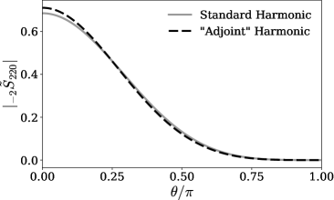
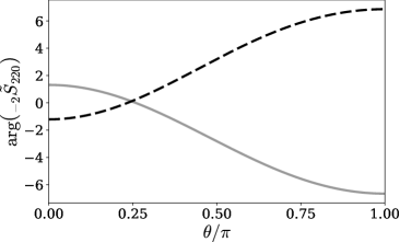
Figure 1: Examples of this work’s central result for spin weight $-2$, and Kerr spin parameter of $a=0.7$: The new adjoint-spheroidal harmonics, ${{}_{-2}}\tilde{S}_{{{\ell mn}}}$, differ from the spheroidal harmonics, ${{}_{-2}}{S}_{{{\ell mn}}}$, in subtle but non-trivial ways. Top: a comparison of harmonic amplitudes for $({{\ell}},m,n)=(2,2,0)$. Bottom: a comparison of harmonic phases for $({{\ell}},m,n)=(2,2,0)$. Note that, for ease of presentation, phases have been scaled by a factor of $100$. Here, $\arg(x+iy)=\tan^{-1}(y/x)$.

Spin-weighted spherical harmonics are perhaps the most commonly used functions for describing the angular behavior of gravitational radiation Thorne (1980); Ruiz et al. (2008). They are the simplest known functions fit for this purpose Thorne (1980). Their completeness and orthonormality make them straightforward to use Breuer et al. (1977). Nevertheless, the spin weighted spherical harmonics are not always the most physically appropriate choice.

This is readily seen in the study of single perturbed black holes (BHs), where the analytic structure of gravitational radiation is understood in terms of the system’s natural modes (eigenfunctions of Einstein’s equations) Teukolsky (1973); Ruiz et al. (2008); London et al. (2014). On one hand, linear perturbations of spherically symmetric spacetimes (e.g. Schwarzschild BHs) are known to yield radiative modes whose angular behavior is spherical harmonic Leaver (1985); Ruiz et al. (2008); Thorne (1980). On the other hand, linear perturbations of spacetimes with angular momentum (e.g. Kerr BHs) are known to yield radiative modes whose angular behavior is spheroidal harmonic Hughes (2000); Leaver (1985); London et al. (2014, 2018); Teukolsky (1973); Holzegel and Smulevici (2013); Berti et al. (2006a); Berti and Klein (2014). There, due to the complete and orthogonal nature of spherical harmonics, spherical harmonic multipole moments may indeed be used to represent gravitational radiation. However, doing so obscures the necessarily simpler information in the system’s natural spheroidal modes Kelly and Baker (2013); London et al. (2014); García-Quirós et al. (2020); Berti and Klein (2014).

The use of spherical harmonics is known to complicate the morphology of gravitational wave signal models, with downstream impact on data analysis  London et al. (2014); García-Quirós et al. (2020); Blackman et al. (2017); Mehta et al. (2019); Carullo et al. (2018); Ghosh et al. (2016); Ota and Chirenti (2020); Bhagwat et al. (2020). In particular, the artificial “mixing” of spheroidal modes is a potentially unnecessary complication, with direct impact on models binary black hole (BBH) merger and ringdown London et al. (2014); García-Quirós et al. (2020); Blackman et al. (2017); Berti and Klein (2014); Kelly and Baker (2013). The need to overcome such complications drives ongoing interest in representing gravitational waves using harmonics that are as closely as possible related to the system’s natural modes Holzegel and Smulevici (2013); García-Quirós et al. (2020); London et al. (2018, 2014).

In this context, spheroidal harmonics represent a logical alternative to spherical harmonics. They are used extensively in black hole perturbation theory, and are integral to the calculation of gravitational waves from extreme mass-ratio inspirals Hughes (2000); Mino et al. (1997); O’Sullivan and Hughes (2014). However, spheroidal harmonics have not been used more broadly in Post-Newtonian (PN) theory or Numerical Relativity (NR), in part, for technical reasons.

In the late inspiral, merger and ringdown of extreme or comparable mass-ratio BH coalescence, spheroidal harmonics are the complex valued, non-orthogonal eigenfunctions of Einstein’s equations, which are themselves non-hermitian in these regimes Hughes (2000); Blanchet (2014); Teukolsky (1973); Leaver (1985). Due in part to these features, it has thus far not been shown whether spheroidal harmonics possess the key properties that make spherical harmonics so useful: completeness (the ability to exactly represent arbitrary gravitational wave signals), and orthogonality (the ability to decompose gravitational wave signals into independent moments of information).

Here, we will see how these technical hurdles can be overcome. The primary result of this work is a class of new special functions that we will call the adjoint-spheroidal harmonics. They are related to the complex conjugates of the regular spheroidal harmonics, but differ from them in important ways. For example, Fig. 1 shows that the absolute values of adjoint harmonics differ nontrivially from the traditional spheroidal harmonics. In this work we lay the mathematical foundation for the adjoint-spheroidal harmonics. For the first time we show that they are complete when defined over the Quasi-Normal Modes (QNMs), and that they exhibit a kind of orthogonality in that setting. These properties are naturally connected to the existence of the adjoint-spheroidal harmonics.

In a companion paper (Paper II, Ref. London (2021)), we present example applications of the adjoint-spheroidal harmonics to gravitational waves from extreme and comparable mass-ratio BBHs, and we discuss potential applications of the adjoint-spheroidal harmonics in gravitational wave theory.

Although our presentation will focus on linear gravitational perturbations of Kerr, their QNMs, and thus their related spheroidal harmonics Leaver (1985), we expect that the mathematical structure of our results applies (exactly or approximately) to any spin weighted harmonics related to the modes of axisymmetric spacetimes with angular momentum.

For simplicity, we consider only spheroidal harmonics corresponding to pro- or retrograde QNMs (i.e. exclusively pro- or retrograde perturbations with respect to the BH spin). The resulting adjoint-spheroidal harmonics can be used to calculate spheroidal harmonic multipole moments via bi-orthogonal decomposition, i.e. orthogonality between two sets of functions rather than one Brauer (1964); Christensen (2003). Like the spin-weighted spherical harmonics, the spin-weighted spheroidal and adjoint-spheroidal harmonics allow the representation of general gravitational wave signals. Unlike the spherical harmonics, the spheroidal harmonics and their multipole moments are closely related to the natural modes of stationary spacetimes with angular momentum Leaver (1985); Teukolsky (1973).

We will discuss QNM orthogonality and completeness in the context of only the polar (i.e. $\theta$) dependence of each mode. In this sense, the presented work focuses on the solutions of Teukolsky’s angular equation Leaver (1985); Teukolsky (1973). One could alternatively focus on Teukolsky’s master equation, which describes all spatial dependencies of perturbations, and separates into the radial and angular equations. In that setting, one would be interested in the master equation’s self-adjointness, with respect to an appropriately constructed weight function. From that perspective, as well as what will be investigated here, the underlying premise is that the known uniqueness of QNM eigenvalues ( see Sec. III.1) strongly implies the existence of a (bi-) orthogonal solution space.

Here, we have chosen to investigate this topic by focusing on the angular equation because of its relative simplicity. While this manuscript was being prepared, the author learned of ongoing and complementary work which investigates orthogonality of QNMs from the perspective of the master equation  Green et al. (2022); Sberna et al. (2022). That work, as well as what we present here, are potential first steps towards a more general representation of gravitational radiation that is closely related to a spacetime’s natural modes.

I.1 Resources for this work

The quantitative results of this work may be reproduced using routines from the openly available Python package, positive London et al. (2020). Of principle use are the Kerr QNM frequencies and the spheroidal harmonics. Both of these quantities may be determined using, for example, Leaver’s analytic representation Leaver (1985). In positive, the QNM frequencies may be accessed via the positive.qnmobj class, which automatically collects a QNM’s frequency, spheroidal and radial harmonics. The class contains convenient routines for calculating spherical-spheroidal inner-products, and can be made consistent with various popular QNM conventions (see positive.qnmobj.explain_conventions). Similarly, positive contains multiple inter-consistent routines for calculating the central objects of current interest, the spheroidal harmonic functions. These may be accessed via positive.slm, which uses Leaver’s representation, and positive.slmcg, which uses a spherical harmonic representation. This work’s central result, namely the adjoint-spheroidal harmonics, may be accessed via positive.calc_adjoint_slm_subset.

I.2 Notation & Conventions

We will at times adopt slightly different notations for convenience and brevity, and we will at times bypass mathematically rigorous definitions, language, and structure with the intent of expediting access to physical concepts. Proofs of various key ideas will be left to references Christensen (2003); Brauer (1964); Courant and Hilbert. (1954). We will work under geometrized units $G=c=1$ with $M=1$.

It will very often be useful to discuss different kinds of functions, e.g. different kinds of spheroidal harmonics. In each case, by “kinds”, “vector space”, or “set”, we mean ordered sets of complex valued square-integrable functions which we may treat as abstract vectors.

Outside of introductory sections we will drop the spin weight labels from the harmonics; for example, spheroidal harmonics ${{}_{s}S_{{{\ell mn}}}}$ will be denoted $S_{{{\ell mn}}}$. We will denote the spherical harmonics, ${{}_{s}}Y_{{\ell m}}$, as $Y_{{\ell m}}$. While we will only be concerned with outgoing gravitational radiation (i.e. spin weight $-2$) most aspects of our discussion apply to all spin weights. In discussion where both spherical and spheroidal harmonics are relevant, we will denote spherical harmonic indices with an overbar. We will be centrally concerned with the $\theta$ dependence of each harmonic; thus, $Y_{{\ell}{m}}$ and $S_{\ell mn}$ will refer to $Y_{{\ell}{m}}(\theta)$ and $S_{\ell m}(\theta;\gamma_{\ell mn})$, where $\gamma_{{{\ell mn}}}$ is the QNM’s oblateness.

In some cases, we will consider the oblateness to not depend on $\ell$ and $n$. There, to emphasize the difference between the fixed-oblateness spheroidal harmonics and the physical ones, we will refer to the fixed-oblateness spheroidal harmonics as $Z_{{{\ell m}}}(\theta;\gamma)$.

The reader should note that in both spherical and spheroidal settings, axisymmetry means that $\phi$ dependence of radiation is $e^{im\phi}$. Since $e^{im\phi}$ are orthogonal in $m$, any radiation may be decomposed into moments with like $m$. Thus we will exclusively work in settings where where $m$ is fixed.

Regarding the spheroidal oblateness, we will let $a$ denote the BH spin magnitude per unit mass, $a=J/M$, and $\tilde{\omega}_{{\ell mn}}$ denote the complex valued QNM frequency. This allows the oblateness to be defined as

$$\gamma_{{{\ell mn}}}\;=\;a\,\tilde{\omega}_{{{\ell mn}}}\;,$$ (1)

where $n$ is an overtone label Berti et al. (2006b); Nollert (1999); Andersson (1997). There will be special cases in which multiple overtones are irrelevant; in these cases the overtone label will be dropped, and the oblateness will simply be denoted as $\gamma$ (i.e. it need not be interpreted according to Eq. (1)). Related spheroidal harmonics will be written as $S_{{\ell m}}$ or $S_{{\ell m}}(\theta;\gamma)$.

Sums over indices will always be between some lower bound and infinity unless otherwise stated. For the spherical polar indices, we will use the usual bounds: $\mathrm{max}(|m|,|s|)\leq{{\ell}}<\infty$ and $-{{\ell}}\leq m\leq{{\ell}}$.

Bra-ket notation, ${\langle{\cdot}\,|\,{\cdot}\rangle}$, will frequently be adopted as short-hand for the scalar product. We will use a standard polar inner-product, where the one dimensional integral is performed over $u=\cos(\theta)$,

$${\langle{p}\,|\,{q}\rangle}\;=\;\int_{-1}^{1}\,p(u)^{*}\,q(u)\,\mathrm{d}u\;.$$ (2)

In Eq. (2), $p(u)$ and $q(u)$ are square-integrable functions of $u$, and $p(u)^{*}$ denotes the complex conjugate of $p(u)$. A spheroidal harmonic ket e.g. $|{S_{{\ell mn}}}\rangle$ is effectively short-hand for $S_{{\ell m}}(\theta;\gamma_{{\ell mn}})$, except in the setting of the scalar product. All harmonics are normalized with respect to Eq. (2) unless otherwise stated.

Lastly, we will only discuss sets of functions with like azimuthal index $m$, and spin weight $s$ Newman and Penrose (1966). The identity operator, ${\mathbb{I}}$, will specifically refer to the space spanned by such functions.

I.3 Outline of the Problem

General gravitational wave signals can be represented in terms of spin-weight $-2$ spherical harmonic multipole moments, but here we wonder if another, perhaps more physical route is possible. If we denote an arbitrary gravitational wave signal (i.e. strain Blanchet (2014)) as $h(r,t,\theta,\phi)$, then its spherical harmonic expansion is

$$h(r,t,\theta,\phi)\;=\;\frac{1}{r}\;\sum_{{{\ell}},m}\,h^{Y}_{{{\ell}}m}(t)\,{{}_{-2}}Y_{{{\ell}}m}(\theta)\,e^{im\phi}\;.$$ (3)

In Eq. (3), $r$ is the radiation’s luminosity distance, $\theta$ and $\phi$ are polar and azimuthal angles describing an observer’s orientation with respect to a source centered frame, and $h^{Y}_{{{\ell}}m}(t)$ is the signal’s spherical harmonic multipole moment Ruiz et al. (2008); Blanchet (2014); London et al. (2018).

Here we will interpret the natural starting point for Eq. (3) to be that the spherical harmonics are naturally related to the QNMs of non-spinning (spherically symmetric) spacetimes Ruiz et al. (2008); Leaver (1985). In that context, $h^{Y}_{{{\ell}}m}(t)$ is naturally a sum over possible overtone contributions Andersson (1997); Leaver (1985). Each overtone QNM ultimately originates from the radial part of the linearized Einstein’s equations, and the physical situation’s initial data determines how much each overtone is excited Leaver (1985); London et al. (2014); Andersson (1997). For general gravitational wave signals, $h^{Y}_{{{\ell}}m}(t)$ may be understood to encode information about the structure and dynamics of the spacetime, including the source Blanchet (2014); Thorne (1980). Despite only corresponding to the modes of spherically symmetric spacetimes, it is well known (e.g. from Sturm-Liouville theory) that the spin-weighted spherical harmonics are complete, orthogonal, and thereby readily applicable to general gravitational wave signals Courant and Hilbert. (1954).

Here, our primary goal is to understand whether the spheroidal harmonics are also applicable to general gravitational wave signals, thereby justifying a spheroidal harmonic multipole moment expansion of the form

$$h(r,t,\theta,\phi)\;=\;\frac{1}{r}\;\sum_{\ell,m}\,h^{S}_{\ell m}(t)\,{{}_{-2}}S_{\ell m}(\theta;\gamma_{\ell m})\,e^{im\phi}\;.$$ (4)

In Eq. (4), $h^{S}_{\ell m}(t)$ are spheroidal harmonic multipole moments, and $\gamma_{\ell m}$ are their closely related oblateness parameters. Note that, like in the case of perturbed spherically symmetric spacetimes, for perturbed Kerr BHs, each $h^{S}_{\ell m}(t)$ may contain information about multiple overtone modes.

In the present work we seek to understand whether Eq. (4) is physically well motivated and mathematically well defined. In Paper II we seek to understand whether the relationship $h^{S}_{\ell m}$ and spacetime modes (e.g. QNMs) makes them useful tools for gravitational wave astronomy London (2021).

Here, we will work through the following technical questions:

1. It is well known that the spheroidal harmonics depend on an oblateness parameter (Eq. 1). In this way, each spheroidal harmonic with polar and azimuthal quantum numbers $\ell$ and $m$ also depends on additional information: the spacetime angular momentum, and the mode frequency which encodes information about the spacetime’s radial structure. What consequences does this additional information have for how we must think about the differential equations which define the QNMs’ spheroidal harmonics?

2. Can the spheroidal harmonics be used to exactly represent arbitrary gravitational wave signals, particularly during e.g. BBH post-merger, but also during merger and inspiral? Equivalently, are the QNMs’ spheroidal harmonics complete?

3. Do the QNMs’ spheroidal harmonics possess a kind of orthogonality?

In forthcoming sections our task is to answer each of these questions.

Along the way we will find that several ideas are intertwined. Whether the spheroidal harmonics are complete is inseparable from how one defines Eq. (4)’s oblateness parameters, $\gamma_{\ell m}$. Completeness of the spheroidal harmonics is sufficient to justify the existence of the adjoint-spheroidal harmonics, and the spheroidal harmonic multipole moments are well defined when the adjoint-spheroidal harmonics are themselves well defined. This work concludes with a discussion of the adjoint-function’s application in the representation of gravitational waves. BH ringdown is chosen as a simple and concrete setting for this discussion. The application of adjoint spheroidal functions to gravitational radiation from the inspiral, merger, and ringdown of extreme and comparable mass ratio BBHs is the subject of Paper II London (2021).

In Sec. II we address question (i), for which a pedagogical review of the spheroidal harmonic differential equation is useful. In short, the differential operator for which the spheroidal harmonics, or simply “spheroidals”, are eigenfunctions can be shown to result from Einstein’s equations linearized about the Kerr solution (i.e. Teukolsky’s equations) Teukolsky (1973); Leaver (1985). For the QNMs, each spheroidal harmonic differential operator depends on the mode’s oblateness, $\gamma_{{\ell mn}}=a\,\tilde{\omega}_{{\ell mn}}$, according to

$$\mathcal{L}_{{{\ell mn}}}=V_{S}(u,\gamma_{{{\ell mn}}})+\partial_{u}(1-u^{2})\partial_{u}\;,$$ (5)

where, $u=\cos{\theta}$, and the operator’s potential is

$$V_{S}(u,\gamma_{{{\ell mn}}})\;=\;s+u\gamma_{{{\ell mn}}}(u\gamma_{{{\ell mn}}}-2s)-\frac{(m^{\prime}+su)^{2}}{1-u^{2}}\;.$$ (6)

In Eq. (6), $s$ is the field’s spin weight, and $m^{\prime}$ is the equation’s analog of the associated Legendre index.

Since each QNM corresponds to a different oblateness, each physical spheroidal harmonic is the eigenfunction of a different differential operator. In turn, each operator is of the associated Legendre type, with a potential given by Eq. (6). Therefore each operator has its own set of eigenfunctions which we may label in ${{\ell^{\prime}}}$ and $m^{\prime}$. Our primary interest will be in the solutions for which ${{\ell^{\prime}}}=\ell$ and $m^{\prime}=m$. These are the physical spheroidal harmonics relevant to gravitational wave theory and experiment Leaver (1985); London et al. (2014); Bhagwat et al. (2017); Berti et al. (2006b). We will at times simply refer to these harmonics as the “physical spheroidals”. As there is an infinity of such harmonics, we are ostensibly faced with an infinity of related different differential operators.

This technical aspect of the QNMs does not appear to have been investigated previously, thus in Sec. II we introduce conceptual tools (ideas and notation) that will help us navigate this “issue of many operators” and its related situations. These tools draw upon ideas from functional analysis and quantum mechanics Christensen (2003); Mostafazadeh (2002).

In Sec. III, we use these tools to address questions (ii) and (iii). We will show that subsets of the physical spheroidal harmonics with fixed overtone label can support bi-orthogonality with the adjoint-spheroidal harmonics, and that related subsets can be complete. If we denote the adjoint-spheroidals as $\tilde{S}_{\ell m}(\theta;\gamma_{{\ell mn}})$, then when we refer to them as the bi-orthogonal dual of the spheroidal harmonics, we simply mean that

$$\int_{0}^{\pi}\,\tilde{S}_{\ell m}(\theta;\gamma_{{{\ell mn}}})\,S^{*}_{{{\ell^{\prime}m}}}(\theta;\gamma_{{{\ell^{\prime}mn}}})\,\sin(\theta)\,\mathrm{d}\theta\;\propto\;\delta_{\ell\ell^{\prime}}\;.$$ (7)

These conclusions are supported by two key ideas from functional analysis. The first is that physical spheroidal harmonics with fixed overtone label form a minimal set, meaning that any one spheroidal harmonic cannot be exactly represented by an infinite sum over the others Christensen (2003). The second key idea is that a set of functions can have a bi-orthogonal dual if and only if it is minimal Christensen (2003). The goal of Sec. III is to to discuss each of these ideas for the spheroidal harmonics of Kerr QNMs.

Section III is the most technical section of this work. It is organized into two subsections. Section III.1 combines ideas presented in Sec. II with old and new perturbation theory results to show that the overtone solutions of Kerr are linearly independent, but not minimal. As will be described in Sec. III.1, this means that from the perspective of the angular harmonics, QNMs with the same values of $\ell$ and $m$, but different overtone labels, $n$, do not encode distinct mode information. This is exactly the situation that one should expect from the Schwarzschild QNMs Leaver (1985). The key corollary of this conclusion is that fixed overtone subsets are minimal. They are therefore a simple and useful way to organize mode information.

Given that the physical spheroidal harmonics on a fixed overtone subset are minimal, the existence of the related adjoint-spheroidal harmonics is assured Christensen (2003). While proof of this fact may be found in Ref. Christensen (2003), the end of Sec. III.1 provides a brief conceptual overview. The reader should note that the full proof does not immediately facilitate calculation of the adjoint-spheroidals, but it does allow us to draw conclusions from their existence.

In particular, existence of the adjoint-spheroidal harmonics allows the construction of a unique linear map (an isomorphism) between spherical and spheroidal harmonics. Once again drawing from results in functional analysis (e.g. Brauer (1964)), Sec. III.2 shows that the uniqueness of this “spherical-to-spheroidal” map means that the spheroidal harmonics are complete Christensen (2003). Like the adjoint-spheroidal harmonics, the existence of a spherical-to-spheroidal map is assured by the properties of the spheroidal harmonics, but not in a way that immediately lends to calculation. However, for concreteness, Sec. III.2 illustrates a way to explicitly define spherical-to-spheroidal maps using the standard spherical harmonic expansion along with related raising and lowering operators defined in Ref. Shah and Whiting (2016).

Section IV goes a step further by showing that spherical-to-spheroidal maps may be expressed as infinite dimensional matrices of inner-products. The truncation of these matrices enables practical non-perturbative calculation of the adjoint-spheroidal harmonics. Section IV presents an algorithm to this end. That algorithm is the central result of this work. Numerical examples are provided for the dominant $m=2$ Kerr spheroidal harmonics.

Section V provides a pedagogical discussion of what spheroidal harmonic decomposition might look like in practice. This section completes our discussion of the potential role of overtones within spheroidal harmonic decomposition (Eq. 4). In particular, a quantitative comparison of mode-mixing between spherical and spheroidal representations closes our discussion.

Section VI summarizes our work thus far and points the way to future development.

Appendix (A) provides a perturbation theory derivation of spherical-spheroidal mixing coefficients that provides leading order estimates at arbitrary perturbative orders. Appendix (B) revisits the issue of many operators by introducing two new operators of relevance to the physical spheroidal harmonics. The first operator is one for which all physical spheroidal harmonics are eigenfunctions. The second is an operator for which all adjoint-spheroidal harmonics are eigenfunctions. While this second operator is simply the adjoint of the first, its introduction helps illuminate the role of isospectrality and operator inter-winding in the adjoint-spheroidal harmonics.

II The Issue of Many Operators

Standard arguments for orthogonality and completeness assume that a single operator defines the space of interest. This is true e.g. for the spherical harmonics. But this is not true for the physical spheroidal harmonics, with their oblateness values that depend on $\ell$. Here we briefly work through standard arguments for orthogonality and completeness in the context of a simple kind of spheroidal harmonic wherein all oblateness values are the same for different values of $\ell$ and $m$ (i.e. not the physical spheroidal harmonics). This special case will allow us to briefly review the concepts of orthogonality and bi-orthogonality. We then show why the standard arguments underpinning these concepts do not trivially generalize to the physical spheroidal harmonics. We conclude with a summary of the ideas necessary to generalize the standard arguments to the physical spheroidals.

We will use bra-ket notation to facilitate various manipulations. We will also use different symbols to distinguish the spheroidal harmonics with fixed oblateness from the physical spheroidal harmonics. Thusly we will denote the spheroidal harmonics with fixed oblateness as $Z_{\ell m}(\theta;\gamma)$, and the associated kets as $|{Z_{{\ell m}}}\rangle$. Similarly, we will denote the physical spheroidal harmonics as $S_{\ell m}(\theta;\gamma_{{\ell mn}})$, and the associated kets as $|{S_{{\ell mn}}}\rangle$. The reader should note that, as discussed in the context of Eq. (6), the fixed-oblateness spheroidals are related to the physical spheroidals when the oblateness varies with $\ell$ (and/or overtone label $n$) according to

$${S_{{\ell mn}}}(\theta,\gamma_{{\ell mn}})\;=\;{Z_{{\ell m}}}(\theta,\gamma)|_{\gamma=\gamma_{{\ell mn}}}\;.$$ (8)

Equation (8) communicates that while each $Z_{{\ell m}}$ and $S_{{\ell mn}}$ are closely related, their key difference is whether they are members of a sequence of harmonics in which the oblateness parameter varies between different harmonics in the sequence.

Our current aim is to describe select properties of the fixed-oblateness spheroidals, and by doing so highlight key aspects of physical spheroidals. In this setting, the spheroidal harmonic differential operator is

$${\mathcal{L}_{o}}\;=\;\left(s+u\gamma(u\gamma-2s)-\frac{(m+su)^{2}}{1-u^{2}}\right)+\partial_{u}(1-u^{2})\partial_{u}\;.$$ (9)

The fixed-oblateness spheroidal harmonic kets, $|{Z_{{\ell m}}}\rangle$, are then eigenvectors of ${\mathcal{L}_{o}}$ with eigenvalues $-A_{{\ell m}}$,

$${\mathcal{L}_{o}}\,|{Z_{{\ell m}}}\rangle\;=\;-A_{{\ell m}}\,|{Z_{{\ell m}}}\rangle\;.$$ (10)

In the context of perturbed Kerr BHs, $A_{{\ell m}}$ is the separation constant for Teukolsky’s master equation Teukolsky (1973).

We are now prepared to demonstrate how the properties of ${\mathcal{L}_{o}}$ provide information about the completeness and orthogonality (or as we shall see bi-orthogonality) of the fixed-oblateness spheroidal harmonics. Pedagogical arguments to this end for e.g. the spherical harmonics begin by determining the adjoint of their differential operator, and then analyzing the matrix elements of that operator in a spherical harmonic basis. Here we may proceed in the same manner, but we must take extra care, as $\gamma$ can be complex valued  (e.g. Eq. 5). As a result, the operator adjoint, ${{\mathcal{L}_{o}}}^{\dagger}$, as defined by

$${\langle{p}\,|\,{{\mathcal{L}_{o}}\,|\,q}\rangle}\;=\;{\langle{p}\,|\,{{\mathcal{L}_{o}}\,q}\rangle}\;=\;{\langle{\,{{\mathcal{L}_{o}}}^{\dagger}p}\,|\,{q}\rangle}\;,$$ (11)

can be shown (via integration by parts) to simply be

$${{\mathcal{L}_{o}}}^{\dagger}\;=\;{\mathcal{L}_{o}}^{*}\;.$$ (12)

The first equality of Eq. (11) simply communicates that ${\mathcal{L}_{o}}$ acting on an arbitrary ket $|{q}\rangle$ results in a new ket, $|{{\mathcal{L}_{o}}\,q}\rangle$. Equation (12) is a slight departure from Sturm-Liouville theory which, if $\gamma$ is real, simply yields that ${{\mathcal{L}_{o}}}^{\dagger}={\mathcal{L}_{o}}\;$ (i.e. if $\gamma$ is real, then ${\mathcal{L}_{o}}$ is self-adjoint) Courant and Hilbert. (1954). Equations (12) and (10) can be used to show that

$${{\mathcal{L}_{o}}}^{\dagger}\,|{Z^{*}_{{\ell m}}}\rangle\;=\;-A^{*}_{{\ell m}}\,|{Z^{*}_{{\ell m}}}\rangle\;,$$ (13)

meaning that the eigenvectors of ${{\mathcal{L}_{o}}}^{\dagger}$ are simply conjugates of the spheroidal harmonics.

We are now prepared to write matrix elements of ${\mathcal{L}_{o}}$ in a vector space for which rows are spanned by eigenvectors of ${{\mathcal{L}_{o}}}^{\dagger}$, and columns are spanned by eigenvectors of ${\mathcal{L}_{o}}$. Doing so yields two equivalent expressions:

$${\langle{\,Z^{*}_{{{\ell^{\prime}m}}}}\,|\,{{\mathcal{L}_{o}}\,|\,Z_{{{\ell m}}}}\rangle} ={\langle{\,Z^{*}_{{{\ell^{\prime}m}}}}\,|\,{{\mathcal{L}_{o}}\,Z_{{{\ell m}}}}\rangle}=-A_{{\ell m}}\,{\langle{\,Z^{*}_{{{\ell^{\prime}m}}}}\,|\,{Z_{{{\ell m}}}}\rangle}$$ (14)

and

$${\langle{\,Z^{*}_{{{\ell^{\prime}m}}}}\,|\,{{\mathcal{L}_{o}}\,|\,Z_{{{\ell m}}}}\rangle} ={\langle{{{\mathcal{L}_{o}}}^{\dagger}\,Z^{*}_{{{\ell^{\prime}m}}}}\,|\,{Z_{{{\ell m}}}}\rangle}=-A_{{\ell^{\prime}m}}\,{\langle{\,Z^{*}_{{{\ell^{\prime}m}}}}\,|\,{Z_{{{\ell m}}}}\rangle}\;.$$ (15)

Equation (14) uses the eigenvalue relation for ${\mathcal{L}_{o}}$, while Eq. (15) uses the definition of the adjoint (Eq. 11) and the eigenvalue relation for ${{\mathcal{L}_{o}}}^{\dagger}$. Since Eqs. (14-15) represent the same quantity in two different ways, their difference must be zero. Subtracting Eq. (14) from Eq. (15) yields

$$(\,A_{{\ell^{\prime}m}}-A_{{\ell m}}\,)\;{\langle{\,Z^{*}_{{{\ell^{\prime}m}}}}\,|\,{Z_{{{\ell m}}}}\rangle}\;=\;0\;.$$ (16)

For ${{\ell}}^{\prime}\neq{{\ell}}$, Eq. (16) communicates that ${\langle{\,Z^{*}_{{{\ell^{\prime}m}}}}\,|\,{Z_{{{\ell m}}}}\rangle}\;=\;0\;$ or, equivalently,

$${\langle{\,Z^{*}_{{{\ell^{\prime}m}}}}\,|\,{Z_{{{\ell m}}}}\rangle}\;\propto\;\delta_{{{\ell}}^{\prime}{{\ell}}}\;.$$ (17)

There are many lessons to be learned from this simple example. Broadly, these lessons can help us distinguish between orthogonality, bi-orthogonality, and the relevance of many operators for the physical spheroidal harmonics. These lessons are prerequisites for our ultimately understanding the physical spheroidal harmonics’ bi-orthogonality and completeness.

One lesson pertains to the case of zero oblateness. There, $\gamma=0$, and Eq. (9) can be used to show that ${\mathcal{L}_{o}}$ reduces to the spherical harmonic differential operator. In that setting Eq. (17) reduces to the known fact that the spin-weighted spherical harmonics are orthogonal in ${{\ell}}$ Newman and Penrose (1966).

Another lesson pertains to cases where the oblateness is complex valued. In that case, Eq. (9) means that the spheroidal harmonics with fixed oblateness are not orthogonal with themselves, but rather with their complex conjugates. Because two sets of functions are needed, Eq. (17) is a statement of biorthogonality Brauer (1964); Christensen (2003); Courant and Hilbert. (1954). Thus it is said that the conjugate spheroidal harmonics, $Z^{*}_{{\ell m}}$, are bi-orthogonal duals of $Z_{{\ell m}}$. In particular, we note that Eq. (17) differs from the usual statement of orthogonality due to the presence of $Z^{*}_{{\ell m}}$ rather than $Z_{{\ell m}}$ in its ket. In Sec. III.1, we will begin to generalize this simple kind of bi-orthogonality to the physical spheroidal harmonics. While Eq. (17) is a simple result that has been known to functional analysis for some time (e.g. Refs. Brauer (1964) and Courant and Hilbert. (1954)), this appears to be the first time it has been pointed out in the context of spheroidal harmonics relevant to BHs.

We now turn to the key lesson of Eqs. (14-17), and the motivating issue of this section. Our previous conclusions of orthogonality or bi-orthogonality hinge upon the fact that ${\mathcal{L}_{o}}$ does not depend explicitly on ${{\ell}}$. It is this point that allows us to calculate matrix elements in Eqs. 14 and 17. To examine this point, we may begin to consider the case of the physical spheroidal harmonics and their operators, $\mathcal{L}_{{\ell mn}}$ (i.e. Eqs. 5-6).

Following Eqs. (14-17), we may attempt to write down the matrix elements of $\mathcal{L}_{{\ell mn}}$ using the physical spheroidal harmonics and their conjugates. As with the fixed-oblateness spheroidals, this yields two equivalent expressions:

$${\langle{\,S^{*}_{{{\ell^{\prime}mn}}}}\,|\,{\mathcal{L}_{{\ell mn}}\,|\,S_{{{\ell mn}}}}\rangle} ={\langle{\,S^{*}_{{{\ell^{\prime}mn}}}}\,|\,{\mathcal{L}_{{\ell mn}}\,S_{{{\ell mn}}}}\rangle}$$ (18)

$$=-A_{{\ell mn}}\,{\langle{\,S^{*}_{{{\ell^{\prime}mn}}}}\,|\,{S_{{{\ell mn}}}}\rangle}$$ (19)

and

$${\langle{\,S^{*}_{{{\ell^{\prime}mn}}}}\,|\,{\mathcal{L}_{{\ell mn}}\,|\,S_{{{\ell mn}}}}\rangle} ={\langle{{\mathcal{L}}^{\dagger}_{{\ell mn}}\,S^{*}_{{{\ell^{\prime}mn}}}}\,|\,{S_{{{\ell mn}}}}\rangle}$$ (20)

$$\neq-A_{{\ell^{\prime}mn}}\,{\langle{\,S^{*}_{{{\ell^{\prime}mn}}}}\,|\,{S_{{{\ell mn}}}}\rangle}\;.$$ (21)

Since $\mathcal{L}_{{\ell mn}}$ and $|{S_{{\ell mn}}}\rangle$ have the same oblateness parameter, namely $\gamma_{{\ell mn}}$, Eqs. (18) and (19) simply communicate that $|{S_{{\ell mn}}}\rangle$ is an eigenket of $\mathcal{L}_{{\ell mn}}$. Thus far, this mirrors the result of our special case.

However, since $\mathcal{L}_{{\ell mn}}$ and $|{S_{{\ell^{\prime}mn}}}\rangle$ have different oblateness parameters, namely $\gamma_{{\ell mn}}$ and $\gamma_{{\ell^{\prime}mn}}$, $|{S_{{\ell^{\prime}mn}}}\rangle$ is not an eigenvector of $\mathcal{L}_{{\ell mn}}$. Thus Eq. (20) is not equal to Eq. (21). This turn of events means that standard arguments for orthogonality and bi-orthogonality do not apply to the physical spheroidal harmonics.

One could also investigate the completeness properties of the spheroidal harmonics with fixed oblateness, $Z_{{\ell m}}(\theta,\gamma)$. Since their operator, ${\mathcal{L}_{o}}$, is of Sturm-Liouville form, there is a standard argument in functional analysis to show that $Z_{{\ell m}}(\theta;\gamma)$ form a complete set: The Sturm-Liouville form of ${\mathcal{L}_{o}}$ means that there exists an invertible operator, say ${\mathcal{T}_{o}}$, that transforms spherical harmonics into spheroidal harmonics. As maths go, one may prove that ${\mathcal{T}_{o}}$ exists without showing explicitly how to calculate it Brauer (1964); Christensen (2003). Nevertheless, the existence of ${\mathcal{T}_{o}}$ can then be used to prove that $Z_{{\ell m}}(\theta,\gamma)$ form a complete set. Crucially, as with ${\mathcal{L}_{o}}$, a key assumption is that ${\mathcal{T}_{o}}$ is independent of $\ell$. Thus this standard argument also falls short of applying to the physical spheroidal harmonics. (This line of reasoning will be revisited in Sec. III.2.)

With the breakdown of standard arguments comes questions. Given that we know the QNM frequencies $\tilde{\omega}_{{\ell mn}}$, and therefore the oblatenesses $\gamma_{{\ell mn}}=a\tilde{\omega}_{{\ell mn}}$, we therefore know all of the operators for which the physical spheroidal harmonics are eigenfunctions. Does this not imply that we should be working within a framework that explicitly accounts for the spheroidal harmonics’ multiple operators? In such a framework, what form should the collection of spheroidal harmonic operators take? Is it possible to use this framework to determine whether the physical spheroidals form a complete set? Does this framework shed light on whether there exist functions that, along with the physical spheroidals, form a bi-orthogonal set?

Hints to each of these question may be found in BH perturbation theory, quantum mechanics and functional analysis literature.

Single BH perturbation theory provides algorithms for computing the physical spheroidal harmonics Leaver (1985); Cook and Zalutskiy (2014). In effect, these algorithms provide a computational definition of a single operator, $\mathcal{L}$, for which all physical spheroidals are eigenfunctions, i.e.

$$\mathcal{L}\,|{S_{{\ell mn}}}\rangle\;=\;-A_{{\ell mn}}\,|{S_{{\ell mn}}}\rangle\;\text{ for all }({{\ell}},m,n).$$ (22)

But it appears that this knowledge has never been articulated mathematically rather than algorithmically. In particular, although we may algorithmically understand the action of $\mathcal{L}$, we cannot begin to determine whether it has an adjoint, ${\mathcal{L}}^{\dagger}$, without a better understanding of its precise mathematical form. We revisit the form of $\mathcal{L}$ in Appx. (B).

From quantum mechanics, Ref. Mostafazadeh (2002) studies the properties of operators (Hamiltonians) whose eigenfunctions are bi-orthogonal. There it is useful to work with a vector space representation of operators (i.e. as is typically done in quantum mechanics with the identity operator).

Lastly, in Refs. Brauer (1964); Christensen (2003) (and many others), the existence of a bi-orthogonal dual and the completeness of the related vector space are discussed in the language of functional analysis. In that setting it is known that a sequence of vectors has a bi-orthogonal dual if it is not only linearly independent, but also minimal (in the sense described in Sec. I.3) Christensen (2003).

Our current task is to apply these hints to questions about the physical spheroidal harmonics, and their many operators $\mathcal{L}_{{\ell mn}}$.

III Spheroidal harmonic bi-orthogonality and completeness

Here we work through two problems regarding the bi-orthogonality and completeness of the physical spheroidal harmonics. For concreteness, our discussion will center about the spheroidal harmonics of Kerr QNMs. The first problem to be addressed has to do with how we should conceptualize the QNMs’ spheroidal harmonics. The result of this discussion is in effect an existence proof of the adjoint-spheroidal harmonics. The second problem has to do with the completeness of the physical spheroidal harmonics. Given the existence of the adjoint-spheroidal harmonics, as well as the existence of an operator that maps spherical to spheroidal harmonics, this section concludes that the spheroidal harmonics are complete, and and therefore may be used to represent arbitrary gravitational radiation.

Regarding how the spheroidal harmonics are conceptualized, it is well known that the QNMs of Schwarzschild BHs are naturally organized into spherical harmonic moments, where each may be a sum of overtones,

$$h^{\mathrm{QNM}}_{\mathrm{Schwarzschild}}=\frac{1}{r}\sum_{{{\ell}},m}\left(\sum_{n=0}^{\infty}b_{{{\ell mn}}}\,e^{-i\tilde{\omega}_{{\ell mn}}t}\right){{}_{-2}Y_{{{\ell m}}}}(\theta)\,e^{im\phi}\;.$$ (23)

In Eq. (23), $b_{{{\ell mn}}}$ is a complex valued QNM amplitude, and the net expression describes the QNM part of BH ringdown Leaver (1985). It may be seen in Eq. (23) that for Schwarzschild BHs, every overtone mode labeled with $\ell$ and $m$ has exactly the same angular “shape” given by ${{}_{-2}Y_{{{\ell m}}}}(\theta)$.

The matter would seem to be very different for Kerr QNMs. The oblateness parameter’s appearance in the spheroidal harmonic differential operator (Eqs. 5-6) means that every overtone labeled with $\ell$ and $m$ is associated with a different spheroidal harmonic, ${{}_{-2}S_{{\ell m}}}(\theta;\gamma_{{\ell mn}})$. Restricting our consideration to (exclusively) only pro- or retrograde Kerr QNMs London and Fauchon-Jones (2019); Magaña Zertuche et al. (2021)

$$h^{\mathrm{QNM}}_{\mathrm{Kerr}}=\frac{1}{r}\sum_{{{\ell}},m}\left(\sum_{n=0}^{\infty}b_{{{\ell mn}}}\,e^{-i\tilde{\omega}_{{\ell mn}}t}{{}_{-2}S_{{{\ell m}}}}(\theta;\gamma_{{\ell mn}})\right)\,e^{im\phi}\;,$$ (24)

where we use the convention that

$$\tilde{\omega}_{{{\ell}}mn}\;=\;-\tilde{\omega}_{{{\ell}}\,-m\,n}^{*}\;.$$ (25)

The simplified perspective of Eq. (24) is relevant to e.g. the post-mergers of non-precessing BBHs (e.g. London et al. (2014); Kamaretsos et al. (2012a); Husa et al. (2016); Khan et al. (2016)), and it has been shown to apply to a large variety of precessing systems Hamilton et al. (2021). We will discuss the implications of that simplification in Sec. VI. For now, with Eqs. (23-24) in mind, the key matter of concern is the extent to which it is meaningful to think of different Kerr overtones as having different angular shapes given by ${{}_{-2}S_{{\ell m}}}(\theta;\gamma_{{\ell mn}})$.

In Sec. III.1 we will show that the multiple overtones in Eq. (24) provide redundant angular information. This will be accomplished by an investigation of the harmonics’ large-${{\ell}}$ behavior in three limits: zero oblateness, linear in oblateness, and general oblateness. We will show that, to linear order in $\gamma_{{\ell mn}}$, the spheroidal harmonics become identical to the spherical harmonics as ${{\ell}}\rightarrow\infty$, regardless of overtone number. We will also see that this conclusion generalizes in a simple way to arbitrary values of $\gamma_{{\ell mn}}$. In this sense we will see that the conceptual structure of Eq. (23) prevails – it is not robust to think of the different overtones’ spheroidal harmonics as being distinct from one another.

It is then fair to wonder whether there exists an alternative representation of Eq. (24) that explicitly accounts for redundancy in the overtones’ spheroidal harmonics. In other words, is there a systematic way to organize the physical spheroidal harmonics into minimal (i.e. non-redundant) subsets? While there are surely many mathematical answers to this question, Sec. III.1 adopts an approach that is physically motivated: The fundamental (i.e. $n=0$) QNMs are known to be the most excited, and persist in time domain signals for the longest duration London et al. (2014); Leaver (1985); Berti et al. (2016); Khan et al. (2016); Kamaretsos et al. (2012b). In physical scenarios, such as the nonlinear BBH merger, where it may be possible for higher overtones to play a significant role, it is currently unclear whether QNMs apply at all, given that the background spacetime is changing at its fastest rate in the entire coalescence, strongly implying that it is not stationary and thus not Kerr Keitel et al. (2017). This reasoning motivates our consideration of what we will call fixed overtone subsets of the spheroidal harmonics. In particular, numerical examples in Sec. III.1 provide evidence that the set of $n=0$ spheroidal harmonics is minimal, and thus supports a bi-orthogonal dual.

The reader should note that when we refer to adjoint-spheroidal harmonics we specifically mean those defined on a single overtone subset, and that all numerical results pertain to the $n=0$ subset which is known to be both astrophysically relevant and spectrally stable Jaramillo et al. (2020).

Section III.2 addresses the question of whether physical spheroidal harmonics may, in principle, be used to exactly represent general gravitational wave signals. In this discussion we begin to address the issue of many operators by constructing a spherical to spheroidal map that is appropriate for the physical spheroidal harmonics. We apply this map to a standard argument for completeness, and show that the physical spheroidal harmonics with $n=0$ form a complete set.

While these discussions of bi-orthogonality and completeness rely on functions and operators that have been shown to simply exist without explicit definition, Sec. III.2 provides an approximate expression for the basic spherical to spheroidal map. The reader may look to Sec. IV for a non-perturbative definition of that map, and the adjoint-spheroidal harmonics.

III.1 Minimal spheroidal harmonic subsets

We will now show that overtone subsets are minimal, and therefore support the existence of the adjoint-spheroidal harmonics. By overtone subsets, we mean sets of Kerr spheroidal harmonics where all members have the same overtone index $n$. For example, all spheroidal harmonics with $n=0$ define the “lowest” or “fundamental” overtone subset. By minimal, we mean that

$$|{S_{{\ell^{\prime}mn}}}\rangle\neq\sum_{{{\ell}}\neq{{\ell^{\prime}}}}\,c_{{{\ell}}}\,|{S_{{\ell mn}}}\rangle,\;\text{for all possible }c_{{\ell}}\text{ and }{{\ell^{\prime}}}\;.$$ (26)

Equation (26) expresses that we cannot equate any member of the overtone subset in terms of a linear combination of all other members. While this may remind the reader of linear independence, it should be noted that linear independence strictly applies to sets of finite size, and so is not quite applicable here. In particular, since Eq. (26) sums over ${{\ell}}$ through infinity, we must investigate the spheroidal harmonics in that limit. Our goal is to determine wether a kind of linearly dependent behavior emerges asymptotically.

To proceed, it suffices to apply a standard argument for linear independence, and then consider the limit as ${{\ell}}\rightarrow\infty$ in that context. To show that a finite subset of harmonics is linearly independent, we may rely on a standard lesson from linear algebra: If the eigenvalues of an operator are unique, then that operator’s eigenfunctions are linearly independent. While there exists a standard proof for this statement (e.g. Ref. Axler (2015)), the first half of this section provides a brief overview for transparency and convenience. The latter half of this subsection provides a large-${{\ell}}$ analysis of the spheroidal harmonic eigenvalues, followed by a brief discussion of why minimal sets support bi-orthogonality.

Towards the linear independence of a finite subset of harmonics, we begin in the spirit of contradiction: we may assume that any two spheroidal harmonics, with labels $({{\ell}},m,n)$ and $({{\ell^{\prime}}},m,n^{\prime})$, are linearly dependent,

$$c_{{\ell}}|{S_{{\ell mn}}}\rangle+c_{{{\ell^{\prime}}}}|{S_{{{\ell^{\prime}mn^{\prime}}}}}\rangle=0\;.$$ (27)

We may then apply $\mathcal{L}$ from Eq. (22),

$$A_{{\ell mn}}\,c_{{\ell}}|{S_{{\ell mn}}}\rangle\;+\;A_{{{\ell^{\prime}mn^{\prime}}}}\,c_{{{\ell^{\prime}}}}|{S_{{{\ell^{\prime}mn^{\prime}}}}}\rangle=0\;.$$ (28)

We may also scale Eq. (27) by $A_{{{\ell^{\prime}mn^{\prime}}}}$,

$$A_{{{\ell^{\prime}mn^{\prime}}}}\,c_{{\ell}}|{S_{{\ell mn}}}\rangle\;+\;A_{{{\ell^{\prime}mn^{\prime}}}}\,c_{{{\ell^{\prime}}}}|{S_{{{\ell^{\prime}mn^{\prime}}}}}\rangle=0\;.$$ (29)

Subtracting Eq. (28) from Eq. (29) gives

$$(A_{{\ell^{\prime}mn^{\prime}}}-A_{{{\ell mn}}})\,c_{{\ell}}\,|{S_{{\ell mn}}}\rangle=0\;.$$ (30)

Equation (30) is a key pedagogical step towards our connecting linear dependence to eigenvalues. The left-hand side of Eq. (30) can only be zero if $c_{{\ell}}$ is zero, or $A_{{\ell mn}}$ equals $A_{{{\ell^{\prime}mn^{\prime}}}}$. Equation (27) means that if $c_{{\ell}}$ is zero, then $c_{{\ell^{\prime}}}$ must also be zero; i.e. only trivial linear dependence is possible if eigenvalues are distinct. Thus, if $A_{{\ell mn}}$ and $A_{{{\ell^{\prime}mn^{\prime}}}}$ are distinct, then we must conclude that $c_{{\ell}}$ and $c_{{\ell^{\prime}}}$ are zero, and so $|{S_{{\ell mn}}}\rangle$ and $|{S_{{\ell^{\prime}mn^{\prime}}}}\rangle$ are linearly independent. Whether applied to an arbitrary finite subset of spheroidal harmonics (e.g. one that includes multiple overtones), or specifically to an overtone subset, this argument extends to multiple spheroidals by induction.

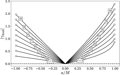
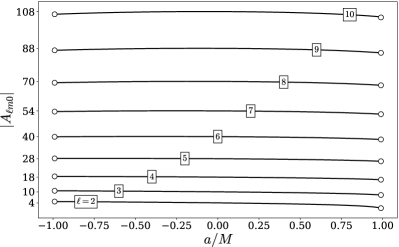
Figure 2: Examples of how physical spheroidal harmonics have distinct oblatenesses for each $\ell$, and that the related eigenvalues are also distinct. Left: The absolute value of oblatenesses for different Kerr BH spins, $a=J/M$, for spin weight $s=-2$, azimuthal index $m=2$, and overtone number $n=0$, and $\ell$ from $2$ to $10$. The horizontal dashed line marks zero oblateness, where the spheroidal harmonics are equal to the sphericals. Open circles signify that extremal BH spins are not shown. Right: Eigenvalues for the left panel’s physical spheroidal harmonics. The $y$-axis of this panel has tick-marks defined by the spherical harmonic eigenvalue, ${{\ell}}({{\ell}}+1)-s(s+1)$.

We now turn to the physical spheroidal harmonics’ eigenvalues ( Eqs. 10 and 22). Our aim is to apply the preceding argument of linear independence to spheroidal harmonics that differ in ${{\ell}}$ and/or $n$. If, for a fixed spin parameter $a$, each $A_{{\ell mn}}$ is distinct as ${{\ell}}\rightarrow\infty$, then the related spheroidal harmonics constitute a set that is not only linearly independent, but also minimal.

The spheroidal harmonic eigenvalues may be calculated to perturbative orders in $\gamma_{{\ell mn}}$ (e.g.  Seidel (1989); Breuer et al. (1977); Press and Teukolsky (1973); Berti et al. (2006a)), or numerically via e.g. Leaver’s method Leaver (1985). We will first use a perturbative approximate to investigate general analytic properties, and then a numerical estimate particular to the $n=0$ spheroidals of Kerr QNMs. For the numerical check, Leaver’s method will be used to compute the QNM frequencies, $\tilde{\omega}_{{\ell mn}}$, from the BH spin parameter, $a$. From this, the oblateness values $\gamma_{{\ell mn}}=a\tilde{\omega}_{{\ell mn}}$ will be used to calculate $A_{{\ell mn}}$ according to Leaver’s algorithm Leaver (1985).

Using the results of Ref. Seidel (1989) to expand $A_{{\ell mn}}$ to second order in $\gamma_{{\ell mn}}$ gives

$$A_{{{\ell mn}}}\; =\;{{\ell}}({{\ell}}+1)-s(s+1)$$ (31a)

$$\;-\;\gamma_{{\ell mn}}\,\frac{2s^{2}m}{\ell(\ell+1)}$$ (31b)

$$\;+\;\gamma_{{\ell mn}}^{2}\,[\;f({{\ell}}+1)-f({{\ell}})-1\;]\;+\;\mathcal{O}(\gamma_{{\ell mn}}^{3}/{{\ell}}^{4})\;,$$ (31c)

where

$$f({{\ell}})\;=\;\frac{\left({{\ell}}^{2}-{{\ell}}_{\min}^{2}\right)\left({{\ell}}^{2}-s^{2}\right)\left({{\ell}}^{2}-\frac{m^{2}s^{2}}{{{\ell}}_{\min}^{2}}\right)}{2\left({{\ell}}-\frac{1}{2}\right){{\ell}}^{3}\left({{\ell}}+\frac{1}{2}\right)}\;,$$ (32)

and ${{\ell}}_{\min}=\mathrm{max}(|m|,|s|)$. Equation (31a) has been written to highlight the perturbative and large-${{\ell}}$ properties of $A_{{\ell mn}}$. The first line of Eq. (31a) is simply the spherical harmonic eigenvalue. Equation (31b) shows the first order correction in $\gamma_{{\ell mn}}$, and Eq. (31c) shows the 2nd order correction along with the order of the remainder. In Eq. (31c) we have taken care to note that the dominant part of the remainder is proportional to both $\gamma_{{\ell mn}}^{3}$ and $\ell^{-4}$. Similarly, higher order corrections are inversely proportional to ${{\ell}}$ at increasing powers Seidel (1989).

We may now use Eqs. (31a-32) to inspect the large-${{\ell}}$ behavior $A_{{\ell mn}}$. The spherical harmonic eigenvalues are distinct in ${{\ell}}$ but degenerate in $n$, thus the same is true for the contribution shown in Eq. (31a). Equation (31b) and Eq. (31c)’s last term vanish as ${{\ell}}\rightarrow\infty$, and an asymptotic expansion of Eq. (31c)’s $\gamma_{{\ell mn}}^{2}$ term shows that its asymptote is $-\gamma_{{\ell mn}}^{2}/2$. In particular, it is not hard to show that as $\ell\rightarrow\infty$,

$$f(\ell+1)-f(\ell)-1 \sim-\frac{1}{2}+\mathcal{O}(\ell^{-2})\;.$$ (33)

Together these points constrain the large-${{\ell}}$ (i.e. asymptotic) behavior of the eigenvalues,

$$A_{{\ell mn}}\;\sim\;{{\ell}}({{\ell}}+1)-s(s+1)-\gamma_{{\ell mn}}^{2}/2\;.$$ (34)

In Eq. (34), “$\sim$” denotes asymptotic equivalence.

As written, Eq. (34) helps us inspect three limits: the zero-oblateness limit, the linear-in-oblateness limit, and the general oblateness limit where the ${{\ell}}$ dependence of $\gamma_{{\ell mn}}$ plays a key role. We will now briefly discuss the spheroidal eigenvalues in each of these contexts.

At $\gamma_{{\ell mn}}=0$, Eq. (34) communicates that the spheroidal eigenvalues are equal to the spherical ones. While this fact is also evident from Eqs. (6) and (31), we emphasize here that the overtone harmonics are neither linearly independent nor minimal for all physically relevant oblatenesses.

We may also draw from Eq. (34) that, at linear order in oblateness, the spheroidal harmonic eigenvalues are equal to the spherical harmonic ones (i.e. one takes $\gamma_{{\ell mn}}^{2}$ to zero at linear order in $\gamma_{{\ell mn}}$). Thus it is not only that the spheroidal harmonics reduce to the spherical harmonics at zero oblateness, but also that in the small oblateness limit, large-${{\ell}}$ spheroidal harmonics have eigenvalues that are asymptotically equivalent to those of the spherical harmonics. Since the spherical eigenvalues only depend on $l$ and $s$, the different overtones’ spheroidal harmonic in $n$ are asymptotically equivalent.

Finally, for large but physical values of the oblateness parameter, Eq. (34) helps us imagine scenarios where the ${{\ell}}$ dependence of $\gamma_{{\ell mn}}$ plays a central role. For this we may draw from the fact that $\gamma_{{\ell mn}}=a\,\tilde{\omega}_{{\ell mn}}$, and that the QNM frequencies, $\tilde{\omega}_{{\ell mn}}$, are known (e.g. from Ref. Yang et al. (2012)) to have the following large-${{\ell}}$ form

$$\tilde{\omega}_{{\ell mn}}\;\sim\;{{\ell}}\,\omega_{\mathrm{Orb}}+ig_{L}(n+1/2)\;.$$ (35)

In Eq. (35), $\omega_{\mathrm{Orb}}$ is the Keplerian orbital frequency for a circular photon orbit, and $g_{L}$ is related to the Lyapunov exponent of that orbit. For simplicity, we have written Eq. (35) to only the dominant terms in ${{\ell}}$. It is important to note that both $\omega_{\mathrm{Orb}}$ and $g_{L}$ are geometric quantities, and are thus independent of ${{\ell}}$. It is also important to note that $n$ appears in Eq. (35) additively with respect to ${{\ell}}$, meaning that for finite $n$, as ${{\ell}}\rightarrow\infty$, $n$ becomes fractionally insignificant.

With Eq. (35) in hand, we may now consider the regime where ${{\ell}}$ is large with respect to $n$ for $n\geq 0$, and the ${{\ell}}$ dependence of $\gamma_{{\ell mn}}$ dominates (i.e. where ${{\ell}}\gg n$ ). There, the $n$-dependent terms in Eq. (35) may be neglected, yielding

$$\tilde{\omega}_{{\ell mn}}\;\sim\;{{\ell}}\,\omega_{\mathrm{Orb}}\;.$$ (36)

When combined with Eq. (34), the asymptotic behavior Eq. (36) allows us to further distill the large-${{\ell}}$ behavior of the spheroidal eigenvalues. Keeping only the largest powers of ${{\ell}}$, this yields

$$A_{{\ell mn}}\;\sim\;{{\ell}}^{2}\,(1-a^{2}\,\omega_{\mathrm{Orb}}^{2}/2\,)\;.$$ (37)

Thus, in the large-${{\ell}}$ limit, and for large and physical values of oblateness, $A_{{\ell mn}}$ asymptotically lose their dependence on the overtone index $n$. In other words, the related overtones’ spheroidal harmonics become (again) asymptotically equivalent: for any two overtone harmonics with label $n$ and $n^{\prime}$ (and like values of $s$ and $m$), there always exists some ${{\ell}}\gg n$ and ${{\ell}}\gg n^{\prime}$, such that $1-|A_{{\ell mn}}/A_{{{\ell mn}}^{\prime}}|$ is arbitrarily small.

From these three settings (zero-oblateness, linear-in-oblateness, and general oblateness), we may conclude that the standard argument for linear independence holds for different overtones if ${{\ell}}$ is finite, but does not hold as ${{\ell}}\rightarrow\infty$. This is because different overtones with the same value of ${{\ell}}$ have the same asymptotic (i.e. large-$\ell$) behavior. As a result, the full set of spheroidal harmonics, including all overtones, is not minimal according to the infinite sum in Eq. (26). Conversely, and perhaps more importantly, we may also conclude that any subset of physical spheroidal harmonics for which every value of ${{\ell}}$ uniquely labels one harmonic is minimal according to Eq. (26). In what follows we take that the simplest and most physically relevant minimal subset is that with $n=0$ (i.e. the fundamental QNM subset).

Figure 2 graphically demonstrates that, for all allowed spin parameters $a$, the $n=0$ Kerr oblatenesses are distinct, and so are their related eigenvalues. While it is known that values of $\ell$ between $2$ and $5$ are more than sufficient to accurately represent gravitational radiation for current ground based detectors (e.g. London et al. (2018); Blackman et al. (2017); Blanchet (2014); Cotesta et al. (2018)), Fig. 2 shows up to ${{\ell}}=10$ as might be relevant for future detectors. The left and right panels plot quantities with respect to the spin parameter, $a$. We use the convention that $a<0$ corresponds to perturbations that are retrograde to the BH spin direction  Husa et al. (2016); London and Fauchon-Jones (2019). By the convention used in e.g. Ref. Berti and Klein (2014), our $a<0$ corresponds to $m<0$. In the left panel of Fig. 2, the sharp feature about $a=0$ corresponds to $\gamma_{{\ell mn}}$ passing through zero and being (approximately) negated. The absolute value of $\gamma_{{\ell mn}}$ is plotted; the sharp feature simply indicates reflection. The underlying real and imaginary parts of $\gamma_{{\ell mn}}$ are smooth functions of $a$ London and Fauchon-Jones (2019); Husa et al. (2016). Outside of $|a|\approx 0$, it is clear that for the QNMs shown, $|\gamma_{{\ell mn}}|$ are distinct in ${{\ell}}$.

The right panel of Fig. 2 shows the absolute value of spheroidal eigenvalues derived from $\gamma_{{\ell mn}}$ in the right panel of Fig. 2 using Leaver’s method Leaver (1985). The $y$-axis’ tick marks are defined by the spherical harmonic eigenvalues. By comparing the $y$-axis’ tick-marks to the curves for each eigenvalue, it is clear that the spherical harmonic contribution to each eigenvalue dominates. For each spin value shown, each $n=0$ eigenvalue is distinct, supporting the minimal nature of the fundamental QNM subset for all spins.

Having reviewed the minimal nature of overtone subsets, what remains is to understand the connection between a minimal subset and the existence of that subset’s bi-orthogonal dual (i.e. the adjoint-spheroidal harmonics). The claimed connection is that the physical spheroidal harmonics of overtone subsets, $|{S_{{\ell mn}}}\rangle$ (where only ${{\ell}}$ varies), have bi-orthogonal duals, $|{\tilde{S}_{{\ell mn}}}\rangle$, if and only if the overtone subset is minimal. Although we refer the reader to Ref. Christensen (2003) for the full proof of this statement, we conclude this section by outlining the proof’s key ideas.

The claim has two assertions: (i) that $|{\tilde{S}_{{\ell mn}}}\rangle$ exist if $|{S_{{\ell mn}}}\rangle$ are minimal, and (ii) if $|{S_{{\ell mn}}}\rangle$ are minimal, then $|{\tilde{S}_{{\ell mn}}}\rangle$ exist. The proof in question must address each of these assertions separately.

Assertion (i) is perhaps the simplest to demonstrate, as the bi-orthogonality of $|{\tilde{S}_{{\ell mn}}}\rangle$ and $|{S_{{\ell mn}}}\rangle$ mean that

$${\langle{S_{{\ell mn}}}\,|\,{\tilde{S}_{{\ell^{\prime}mn}}}\rangle}\;\propto\;\delta_{{{\ell}},{{\ell^{\prime}}}}\;.$$ (38)

This idea is then applied to the notion of whether any data that can be exactly represented in a linear combination of $|{S_{{\ell mn}}}\rangle$ may also be exactly represented using $|{\tilde{S}_{{\ell mn}}}\rangle$. In particular, it can be shown that Eq. (38) means that $|{S_{{\ell mn}}}\rangle$ cannot be represented as a linear combination of the remaining spheroidals with ${{\ell}}\neq{{\ell^{\prime}}}$. This statement is equivalent to Eq. (26). Thus, if bi-orthogonal duals exist, then the related set is minimal.

The proof of assertion (ii) is somewhat more technical. It can be shown that the right-hand-side of Eq. (26) is related to a projection operator, $\mathcal{U}_{{\ell}}$, which projects a ket onto the space of all spheroidal harmonics with the exception of $|{S_{{\ell mn}}}\rangle$. Note that $\mathcal{U}_{{\ell}}$ is labeled by the same value of $\ell$ as $|{S_{{\ell mn}}}\rangle$. By definition, $\mathcal{U}_{{\ell}}$ is such that ${\langle{S_{{\ell^{\prime}mn}}}\,|\,{({\mathbb{I}}-\mathcal{U}_{{\ell}})\,S_{{\ell mn}}}\rangle}\propto\delta_{{{\ell^{\prime}}},{{\ell}}}$, meaning that $|{\tilde{S}_{{\ell mn}}}\rangle\propto|{({\mathbb{I}}-\mathcal{U}_{{\ell}})\,S_{{\ell mn}}}\rangle$. Thus if $|{S_{{\ell mn}}}\rangle$ are minimal, then $|{\tilde{S}_{{\ell mn}}}\rangle$ exist.

III.2 Maps between spherical and spheroidal harmonics

The existence of the adjoint-spheroidal harmonics means that we may, in principle, decompose arbitrary gravitational wave signals into spheroidal harmonics moments. In this, the right-hand-side of Eq. (4) is justified, and Sec. IV will provide a method to calculate the adjoint harmonics. For now, a key remaining issue is whether we may generally equate any square-integrable gravitational wave signal with its spheroidal harmonic decomposition. In other words, the current topic of discussion is whether the physical spheroidal harmonics, and their adjoint-functions, are complete.

It is useful to frame this topic with a few pedagogical ideas: The spin-weighted spherical harmonics are known to be complete because they are closely related to the trigonometric functions, and the trigonometric functions themselves are known to be complete in a rudimentary way (e.g. the Fourier series) Courant and Hilbert. (1954); Brauer (1964). Completeness of the spherical harmonics means that any square-integrable gravitational wave signal (ket), say $|{h}\rangle$, may be equated with,

$$|{h}\rangle\;=\;\sum_{{{\ell}}}\,|{Y_{{{\ell}}m}}\rangle{\langle{Y_{{{\ell}}m}}\,|\,{h}\rangle}\;.$$ (39)

Equivalently, we may define an identity operator in terms of the spherical harmonics,

$${\mathbb{I}}\;=\;\sum_{{\ell}}\,\,|{Y_{{{\ell}}m}}\rangle\langle{Y_{{{\ell}}m}}|\;,$$ (40)

such that Eq. (39) can be compactly written as $|{h}\rangle={\mathbb{I}}\,|{h}\rangle$. In this language, our present task is to determine whether the identity operator in Eq. (40) may be alternatively represented in terms of the physical spheroidal harmonics and their adjoint functions,

$${\mathbb{I}}\;=\;\sum_{{{\ell}}}\,|{S_{{\ell mn}}}\rangle\langle{\tilde{S}_{{\ell mn}}}|\;.$$ (41)

In Eq. (41), the reader should note that ${\mathbb{I}}$ is specifically the identity operator for all functions (e.g. parts of gravitational wave signals) corresponding to a fixed $m$ and $s$.

To proceed, we will first rely on a standard argument from functional analysis applied to the fixed-oblateness harmonics, $|{Z_{{{\ell}}m}}\rangle$. This argument essentially says that the mean difference between the spherical and spheroidal harmonics is proportional to $1/{{\ell}}$, and so the two harmonics are “close” and as so have related properties. These related properties are defined by a linear operator that maps between spherical and spheroidal harmonics. In this section we will focus on how the existence of such a map means that the physical spheroidal harmonics inherit completeness from the sphericals. The details of supporting arguments are left to the appendix.

In particular, that the spherical and spheroidal harmonics are close is shown in Appx. (A). There, perturbative and recursive methods are used to show that any spheroidal harmonic may be written as a sum of spherical harmonics,

$$|{Z_{{\ell m}}}\rangle\;=\;c_{{{\ell}}}\,|{Y_{{\ell m}}}\rangle\;+\;c_{{{\ell}}}\,\sum_{{{\ell^{\prime}}}\neq{{\ell}}}\,\sigma_{{{\ell^{\prime}}}{{\ell}}}\,|{Y_{{{\ell^{\prime}}}m}}\rangle\;,$$ (42)

where $c_{{{\ell}}}$ is a normalization constant, and

$$\sigma_{{{\ell^{\prime}}}{{\ell}}}\; =\;{\langle{Y_{{{\ell^{\prime}}}m}}\,|\,{Z_{{\ell m}}}\rangle}$$ (43)

$$\approx\;\frac{1}{|{{\ell^{\prime}}}-{{\ell}}|!}\,\left(\frac{-\gamma s}{2{{\ell}}}\right)^{|{{\ell^{\prime}}}-{{\ell}}|}\;.$$ (44)

Equation (42) is simply a spherical harmonic expansion. Equation (44) results from recognizing that perturbation theory has an inherently recursive structure which, in the case of the spherical-spheroidal inner-products, has an exact solution at leading order. The form of Eq. (44) is key as it relates to the general convergence of Eq. (42), and (see e.g. Ref. Brauer (1964)) the existence of an invertible operator, ${\mathcal{T}_{o}}$, that maps spherical to spherical harmonics,

$${\mathcal{T}_{o}}\,|{Y_{{{\ell}}m}}\rangle\;=\;|{Z_{{{\ell}}m}}\rangle\;.$$ (45)

It is the existence and invertibility of ${\mathcal{T}_{o}}$ that can be used to show that the spheroidal harmonics with fixed oblateness, $\gamma$, inherit the completeness of the spherical harmonics Brauer (1964); Christensen (2003).

We are presently concerned with generalizing the arguments of e.g. Ref. Brauer (1964) to the $n=0$ physical spheroidal harmonics to show that they too are complete, and can therefore exactly represent arbitrary gravitational wave signals. This will be done by defining an operator for the physical spheroidals, ${\mathcal{T}}$, that is the generalization of ${\mathcal{T}_{o}}$. Together ${\mathcal{T}_{o}}$, ${\mathcal{T}}$, and their inverses, ${\mathcal{V}_{o}}$ and ${\mathcal{V}}$, will play central roles in our showing that the spheroidals are complete,

$${\mathbb{I}}\;=\;\sum_{{{\ell}}}\,|{S_{{\ell mn}}}\rangle\langle{\tilde{S}_{{\ell mn}}}|\,\;.$$ (46)

Per discussion in Sec. III.1, Eq. (46) is defined for fixed $n$. As implied by Eq. (46), a key component of our discussion will be the fact that adjoint-spheroidal harmonics may exist on overtone subsets.

Let us begin. Given the closeness of the spherical and spheroidal harmonics (e.g. Eq. 44), we may be assured that there exists a linear operator ${\mathcal{T}_{o}}$ that transforms spherical harmonics into spheroidals Christensen (2003); Brauer (1964). For now we need only know that such an operator exists. Nevertheless, it may be worthwhile to briefly discuss its construction. For example, it must be the case that ${\mathcal{T}_{o}}$ acts on $|{Y_{{\ell m}}}\rangle$ to exactly the effect of Eq. (42)’s right hand side. It is also true that spherical harmonics with different values of ${{\ell}}$ are related by linear differential “raising” and “lowering” operators Shah and Whiting (2016). Combining these ideas allows us to think of ${\mathcal{T}_{o}}$ as a kind of differential operator. If we let $\mathcal{P}_{{\ell}}$ and $\mathcal{Q}_{{\ell}}$ be the ${{\ell}}$ raising and lowering operators (Eqns. 29 and 30 of  Ref.Shah and Whiting (2016)) then,

$${\mathcal{T}_{o}}\;\approx\;c_{{\ell}}\;(1\;+\;\sigma_{{{\ell}}-1,{{\ell}}}\,\mathcal{Q}_{{\ell}}\;+\;\sigma_{{{\ell}}+1,{{\ell}}}\,\mathcal{P}_{{\ell}}\,)\;,$$ (47)

with

$$\mathcal{Q}_{{\ell}}\,Y_{{\ell m}}\;=\;Y_{{{\ell}}-1,m}\;\text{ and }\;\;\mathcal{P}_{{\ell}}\,Y_{{\ell m}}\;=\;Y_{{{\ell}}+1,m}\;.$$ (48)

In Eq. (48) the raising and lowering operators are of the form $c_{0}(\theta)+c_{1}(\theta)\,\partial_{\theta}$ Shah and Whiting (2016). In Eq. (47) we have only kept the adjacent spherical harmonic contributions for simplicity. We will see in Sec. IV that it is much more useful to think of ${\mathcal{T}_{o}}$ as an infinite dimensional matrix whose elements are simply related to spherical-spheroidal inner products $\sigma_{{{\ell^{\prime}}}{{\ell}}}$.

Given the existence of ${\mathcal{T}_{o}}$, our first task is to determine a generalization for the physical spheroidal harmonics: ${\mathcal{T}_{o}}$ transforms a spherical harmonic into a spheroidal harmonic with fixed oblateness (Eq. 47). Its generalization should transform a spherical harmonic into a physical spheroidal harmonic. The development of this generalization begins with the our recalling that each physical oblateness, $\gamma_{{\ell mn}}$, defines a set of fixed oblateness harmonics. Therefore there exists a sequence spherical-to-spheroidal maps that are essentially ${\mathcal{T}_{o}}$ but parameterized by the different physical oblateness, $\gamma_{{\ell mn}}$. We will refer to each of these maps as ${\mathcal{T}}_{{\ell mn}}$, where

$${\mathcal{T}}_{{\ell mn}}\,|{Y_{{\ell m}}}\rangle\;=\;|{S_{{\ell mn}}}\rangle\;.$$ (49)

Similarly, we will refer to related inverse maps as ${\mathcal{V}}_{{\ell mn}}$, where

$${\mathcal{V}}_{{\ell mn}}\,|{S_{{\ell mn}}}\rangle\;=\;|{Y_{{\ell m}}}\rangle\;.$$ (50)

We are now tasked with determining whether there exists some generalization, say ${\mathcal{T}}$ and ${\mathcal{V}}$, such that

$${\mathcal{T}}\,|{Y_{{\ell m}}}\rangle\;\,\; =\;|{S_{{\ell mn}}}\rangle\text{ for {all} }{{\ell}}\;,$$ (51)

$${\mathcal{V}}\,|{S_{{\ell mn}}}\rangle\; =\;|{Y_{{\ell m}}}\rangle\;\,\text{ for {all} }{{\ell}}\;.$$ (52)

We may consider the following vector space representations

$${\mathcal{T}}\; =\;\sum_{{{\ell^{\prime}}}}\,{\mathcal{T}}_{{\ell^{\prime}mn}}\,|{Y_{{\ell^{\prime}m}}}\rangle\langle{Y_{{\ell^{\prime}m}}}|\;$$ (53)

$$=\;\sum_{{{\ell^{\prime}}}}\,|{S_{{\ell^{\prime}mn}}}\rangle\langle{Y_{{\ell^{\prime}m}}}|\;,$$ (54)

and

$${\mathcal{V}}\; =\;\sum_{{{\ell^{\prime}}}}\,{\mathcal{V}}_{{\ell^{\prime}mn}}\,|{S_{{\ell^{\prime}mn}}}\rangle\langle{\tilde{S}_{{\ell^{\prime}mn}}}|\;$$ (55)

$$=\;\sum_{{{\ell^{\prime}}}}\,|{Y_{{\ell^{\prime}m}}}\rangle\langle{\tilde{S}_{{\ell^{\prime}mn}}}|\;.$$ (56)

In Eq. (53), we have explicitly written ${\mathcal{T}}$ in terms of the objects we wish to generalize, ${\mathcal{T}}_{{\ell^{\prime}mn}}$. In Eq. (54), we apply ${\mathcal{T}}_{{\ell^{\prime}mn}}$ to $|{Y_{{\ell^{\prime}m}}}\rangle$. As represented in Eqs. (53) and (54), ${\mathcal{T}}$ may be easily shown to map spherical harmonics to physical spheroidal harmonics, as expected.

In Eq. (55), we have also written ${\mathcal{V}}$ in terms of the objects we wish to generalize, ${\mathcal{V}}_{{\ell^{\prime}mn}}$. In Eq. (56), we apply the action of ${\mathcal{V}}_{{\ell^{\prime}mn}}$ on $|{S_{{\ell^{\prime}mn}}}\rangle$. As with $\mathcal{L}$, ${\mathcal{V}}$ may be easily shown to have the correct behavior (i.e. Eq. 51) when acting on spheroidal harmonics. In this case, the correct behavior is assured by the existence and bi-orthogonality of the adjoint-spheroidal harmonics, $\tilde{S}_{{\ell mn}}$.

What remains to be shown is whether ${\mathcal{V}}$ is a unique left and right inverse of ${\mathcal{T}}$. To this end, it suffices to evaluate ${\mathcal{T}}{\mathcal{V}}$ and ${\mathcal{V}}{\mathcal{T}}$. From Eqs. (54) and (56), we have that

$${\mathcal{V}}{\mathcal{T}}\; =\;\sum_{{{\ell^{\prime}}},{{\ell}}}\,|{Y_{{\ell^{\prime}m}}}\rangle{\langle{\tilde{S}_{{\ell^{\prime}mn}}}\,|\,{S_{{\ell mn}}}\rangle}\langle{Y_{{\ell m}}}|\;$$ (57)

$$=\;\sum_{{{\ell}}}\,|{Y_{{\ell m}}}\rangle\langle{Y_{{\ell m}}}|\;=\;{\mathbb{I}}\;,$$ (58)

and

$${\mathcal{T}}{\mathcal{V}}\; =\;\sum_{{{\ell^{\prime}}},{{\ell}}}\,|{S_{{\ell mn}}}\rangle{\langle{Y_{{\ell m}}}\,|\,{Y_{{\ell^{\prime}m}}}\rangle}\langle{\tilde{S}_{{\ell^{\prime}mn}}}|\;$$ (59)

$$=\;\sum_{{{\ell}}}\,|{S_{{\ell mn}}}\rangle\langle{\tilde{S}_{{\ell mn}}}|\;.$$ (60)

In Eqs. (57) and (59) we have used the bi-orthogonality and orthogonality of the spheroidal and spherical harmonics. In Eq. (58), we simply find that ${\mathcal{V}}{\mathcal{T}}$ is the identity operator represented in terms of spherical harmonic bras and kets. However, it may not be immediately clear that Eq. (60) is this same identity operator represented with physical spheroidal harmonics. To clarify the matter, it may help to consider that ${\mathbb{I}}^{2}={\mathbb{I}}$, and so

$${\mathbb{I}}\; =\;{\mathcal{V}}{\mathcal{T}}\;{\mathcal{V}}{\mathcal{T}}\;$$ (61)

$$=\;{\mathcal{V}}\left({\mathcal{T}}{\mathcal{V}}\right){\mathcal{T}}\;.$$ (62)

In Eq. (61), we have simply equated the identity operator with its square. In Eq. (62), we have used the associative property of linear operators to group ${\mathcal{T}}$ with ${\mathcal{V}}$. If ${\mathcal{T}}{\mathcal{V}}$ is not ${\mathbb{I}}$, then we might use ${\mathbb{I}}$ to construct a contradiction: ${\mathcal{V}}\,{\mathbb{I}}\,{\mathcal{T}}\neq{\mathcal{V}}\left({\mathcal{T}}{\mathcal{V}}\right){\mathcal{T}}={\mathbb{I}}$, which reduces to ${\mathbb{I}}\neq{\mathbb{I}}$. Clearly, ${\mathbb{I}}={\mathbb{I}}$, so we must conclude that ${\mathcal{T}}{\mathcal{V}}={\mathbb{I}}$, and equivalently

$${\mathbb{I}}\;=\;\sum_{{{\ell}}}\,|{S_{{\ell mn}}}\rangle\langle{\tilde{S}_{{\ell mn}}}|\;.$$ (63)

An alternative but ultimately equivalent argument is that since each physical spheroidal harmonic within an overtone subset is uniquely associated with a single spherical harmonic (via ${\mathcal{T}}_{{\ell mn}}$), ${\mathcal{T}}{\mathcal{V}}$ must transform to the same space as ${\mathcal{V}}{\mathcal{T}}$. Thus if ${\mathcal{V}}{\mathcal{T}}={\mathbb{I}}$, then so must ${\mathcal{T}}{\mathcal{V}}$ Christensen (2003).

In Eq. (63), we have essentially found that overtone subsets of the physical spheroidal harmonics are complete. The ideas and arguments leading to this conclusion have a number of relevant reductions and alternative framings. For example, if we consider the fixed-oblateness spheroidals instead of the physical spheroidals, then it may be shown that Eq. (63) reduces to

$${\mathbb{I}}\;=\;\sum_{{{\ell}}}\,|{Z_{{\ell m}}}\rangle\langle{{Z}^{*}_{{\ell m}}}|\;.$$ (64)

Further, since the identity operator is self-adjoint (i.e. ${\mathbb{I}}={{\mathbb{I}}}^{\dagger}$), we may also conclude that (reversing the location of $\tilde{S}_{{\ell mn}}$ and ${S}_{{\ell mn}}$ yields)

$${\mathbb{I}}\;=\;\sum_{{{\ell}}}\,|{\tilde{S}_{{\ell mn}}}\rangle\langle{S_{{\ell mn}}}|\;.$$ (65)

Similarly, one might redevelop Eqs. (53-63) with the adjoint operators, ${{\mathcal{T}}}^{\dagger}$ and ${{\mathcal{V}}}^{\dagger}$. These may be found by simply adjugating Eqs. (54) and (56),

$${{\mathcal{T}}}^{\dagger}\;=\;\sum_{{{\ell^{\prime}}}}\,|{Y_{{\ell^{\prime}m}}}\rangle\langle{S_{{\ell^{\prime}mn}}}|\;,$$ (66)

$${{\mathcal{V}}}^{\dagger}\;=\;\sum_{{{\ell^{\prime}}}}\,|{\tilde{S}_{{\ell^{\prime}mn}}}\rangle\langle{Y_{{\ell^{\prime}m}}}|\;.$$ (67)

From Eqs. (66-67) it is straightforward to use bi-orthogonality and orthogonality to show that

$${{\mathcal{T}}}^{\dagger}\,|{\tilde{S}_{{\ell mn}}}\rangle\; =\;|{Y_{{\ell m}}}\rangle\;\,\text{ for all }{{\ell}}\;,$$ (68)

$${{\mathcal{V}}}^{\dagger}\,|{Y_{{\ell m}}}\rangle\,\;\; =\;|{\tilde{S}_{{\ell mn}}}\rangle\text{ for all }{{\ell}}\;.$$ (69)

With Eqs. (63-69) we have an abundance of conceptual tools to help us work with and think about the physical spheroidal harmonics. Our next task is to use these tools to non-perturbatively calculate the adjoint spheroidal harmonics.

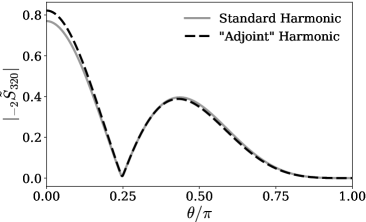
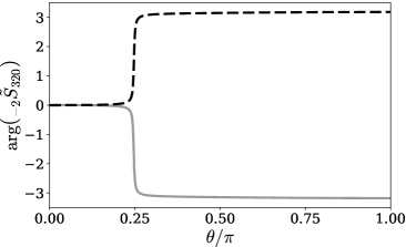
Figure 3: The same as Fig. 1 but for $({{\ell}},m,n)=(3,2,0)$. Examples of this work’s central result for spin weight $-2$, and Kerr spin parameter of $a=0.7$: Top: a comparison of harmonic amplitudes for $({{\ell}},m,n)=(3,2,0)$. Bottom: a comparison of harmonic phases for $({{\ell}},m,n)=(3,2,0)$. Here, $\arg(x+iy)=\tan^{-1}(y/x)$.

IV Calculation of the adjoint-spheroidal harmonics

Here we present a non-perturbative algorithm for calculating the physical adjoint-spheroidal harmonics. The starting point of our discussion is the completeness of the physical spheroidal harmonics on fixed overtone subsets. This result, and related spherical-spheroidal maps, will be used to show that the adjoint-spheroidal harmonics may be calculated using a simple spherical harmonic expansion,

$$|{\tilde{S}_{{\ell mn}}}\rangle\;=\;\sum_{{{\ell^{\prime}}}}\,|{Y_{{\ell^{\prime}m}}}\rangle{\langle{Y_{{\ell^{\prime}m}}}\,|\,{\tilde{S}_{{\ell mn}}}\rangle}\;.$$ (70)

In this, our core task is to determine the inner-product values between spherical and adjoint-spheroidal harmonics, ${\langle{Y_{{\ell^{\prime}m}}}\,|\,{\tilde{S}_{{\ell mn}}}\rangle}$.

We begin by recalling that Eq. (66) provides us with ${{\mathcal{T}}}^{\dagger}$, which transforms adjoint-spheroidal harmonics into spherical ones. We may write ${{\mathcal{T}}}^{\dagger}$ as an infinite dimensional matrix by expanding its spheroidal harmonic bras in spherical harmonics,

$${{\mathcal{T}}}^{\dagger}\;=\;\sum_{{{\ell}},{{\ell^{\prime}}}}\,|{Y_{{\ell^{\prime}m}}}\rangle{\langle{S_{{\ell^{\prime}mn}}}\,|\,{Y_{{\ell m}}}\rangle}\langle{Y_{{\ell m}}}|\;.$$ (71)

Equation (71) simply communicates that, in the spherical harmonic basis, ${{\mathcal{T}}}^{\dagger}$ is simply a matrix of spherical-spheroidal inner-products. For practical numerical calculations, we may consider the $N\times N$ dimensional truncation of ${{\mathcal{T}}}^{\dagger}$,

$${{\mathcal{T}}}^{\dagger}_{(N)}\;=\;\sum_{{{\ell}},{{\ell^{\prime}}}}^{N}\,|{Y_{{\ell^{\prime}m}}}\rangle{\langle{S_{{\ell^{\prime}mn}}}\,|\,{Y_{{\ell m}}}\rangle}\langle{Y_{{\ell m}}}|\;.$$ (72)

In Eq. (72), ${{\ell}}$ and ${{\ell^{\prime}}}$ are between and $\mathrm{max}(|s|,|m|)$ and $N$.

Noting that ${{\mathcal{V}}}^{\dagger}$ is the inverse of ${{\mathcal{T}}}^{\dagger}$, we may use matrix inversion to numerically estimate the matrix elements of ${{\mathcal{V}}}^{\dagger}_{(N)}$, the $N\times N$ truncation of ${{\mathcal{V}}}^{\dagger}$,

$${{\mathcal{V}}}^{\dagger}_{(N)}\; \approx\;{{{\mathcal{T}}}^{\dagger}}^{-1}_{(N)}\;$$ (73)

$$\approx\;\sum_{{{\ell}},{{\ell^{\prime}}}}^{N}\,|{Y_{{\ell^{\prime}m}}}\rangle{\langle{Y_{{\ell^{\prime}m}}}\,|\,{\tilde{S}_{{\ell mn}}}\rangle}\langle{Y_{{\ell m}}}|\;.$$ (74)

In Eq. (73) we denote ${{\mathcal{V}}}^{\dagger}_{(N)}$ as being approximately equal to ${{{\mathcal{T}}}^{\dagger}}^{-1}_{(N)}$, up to truncation error. In Eq. (74), we have expanded Eq. (67)’s adjoint-spheroidal harmonics in sphericals to highlight that the matrix elements of ${{\mathcal{V}}}^{\dagger}_{(N)}$ are the inner-products of interest. In particular, if we denote the matrix elements of ${{\mathcal{V}}}^{\dagger}_{(N)}$ as

$$\tilde{\sigma}_{(N)\,{{\ell^{\prime}}}{{\ell}}}\; =\;\langle{Y_{{\ell^{\prime}m}}}|\,{{\mathcal{V}}}^{\dagger}_{(N)}\,|{Y_{{\ell m}}}\rangle\;,$$ (75)

$$\approx\;{\langle{Y_{{\ell^{\prime}m}}}\,|\,{\tilde{S}_{{\ell mn}}}\rangle}\;.$$ (76)

then the adjoint spheroidal harmonics may be numerically estimated as

$$|{\tilde{S}_{{\ell mn}}}\rangle\; \approx\;\sum_{{{\ell^{\prime}}}}^{N}\;\tilde{\sigma}_{(N)\,{{\ell^{\prime}}}{{\ell}}}\,|{Y_{{{\ell m}}}}\rangle\;.$$ (77)

Equivalently, if we write the adjoint-spheroidals as functions (in full notation) rather than vectors, then

$${{}_{-2}}{\tilde{S}_{{\ell m}}(\theta;\gamma_{{\ell mn}})}\; \approx\;\sum_{{{\ell^{\prime}}}}^{N}\,{{{}_{-2}}Y_{{{\ell m}}}(\theta)}\;\tilde{\sigma}_{(N)\,{{\ell^{\prime}}}{{\ell}}}\;.$$ (78)

Equations (77) and (78) encapsulate the key result of this section. Equation (77) is a way of non-perturbatively calculating the adjoint-spheroidal harmonics, given the spherical-spheroidal inner-products. The approximately diagonal nature of ${{\mathcal{T}}}^{\dagger}$ means that values along the $N^{\mathrm{th}}$ row and column of ${{\mathcal{V}}}^{\dagger}_{(N)}$ are least accurate. In practice, it is found that $N^{\mathrm{th}}$ row and column elements of ${{\mathcal{T}}}^{\dagger}$ rapidly converge with increasing $N$, with $N=\ell+6$ being sufficient to estimate the harmonics to machine precision. An implementation of Eqs. (72-77) is included in positive.aslmcg London et al. (2020).

Figures (1) and (3) show example evaluations of the $({{\ell}},m,n)=(2,2,0)$ and $(3,2,0)$ adjoint-spheroidal harmonics. There each harmonic is normalized when integrated over the solid angle. Prograde QNMs are used (i.e. those with positive QNM frequencies at $m=2$). Each adjoint-harmonic is derived from the $n=0$ overtone subset according to Eq. (77), with $|\ell-\ell^{\prime}|\leq 8$. This choice corresponds to the $|\ell-\ell^{\prime}|=8$ terms’ contributing less than $0.01\%$ in amplitude for each case. Related spheroidal harmonics are calculated from Leaver’s method (i.e. Ref. Leaver (1985)), and positive.physics.qnmobj class has been used to reference QNM frequencies and related spheroidal harmonics with consistent conventions London et al. (2020).

V Spheroidal harmonic decomposition

We have now developed an understanding of why the adjoint-spheroidal harmonics exist, and why an arbitrary gravitational wave signal may be equated with its spheroidal harmonic expansion. While there are still questions of theory within immediate reach, such as whether there exists an operator for which $|{\tilde{S}_{{\ell mn}}}\rangle$ are eigenvectors (See Appx. B), for now, we may begin to focus on somewhat more practical matters. In this section we will be concerned with how one might apply the adjoint-spheroidal harmonics to physical problems.

For simplicity and concreteness we will consider the application of Kerr $n=0$ spheroidal harmonics to arbitrary gravitational wave signals. We will then discuss the specific case of Kerr ringdown (i.e. a sum of QNMs). Lastly, we will discuss the conditions for which a signal’s spheroidal multipole moments may be exactly equated with the physical system’s modes.

Let’s begin by considering the basic situation of gravitational wave theory wherein we wish to represent a gravitational wave signal, $h(r,t,\theta,\phi)$, in terms of radiative multipole moments. In the case of e.g. PN theory, one might want to analytically relate the radiative multipole moments of $h$ to the source’s multipole moments Blanchet (2014); Thorne (1980). In the case of NR, including the numerics of particle perturbation theory, one might be provided with numerical radiation, and then want to decompose that data into multipole moments that are useful for e.g. the development of signal models Hughes et al. (2019); London (2020); Cotesta et al. (2018); Blackman et al. (2017); García-Quirós et al. (2020); London et al. (2018). At the intersection of perturbative and non-perturbative gravitational wave theory, one might want to represent the information perturbing an isolated BH in a way that is closely aligned with the BH’s intrinsic modes Le Tiec et al. (2010); London (2020); Kelly and Baker (2013); García-Quirós et al. (2020). In all of these settings, a spheroidal harmonic representation is of potential use. For each, a choice of oblateness must be made prior to pursuing a spheroidal harmonic decomposition.

In principle, the oblatenesses may be developed to suit the specific physical problem. For example, the Kerr $n=0$ spheroidal harmonics have oblatenesses determined by the BH spin parameter $a$, and the pro- or retrograde QNM frequencies $\tilde{\omega}_{{{\ell mn}}}$. In that setting oblateness values are ordered by ${{\ell}}$, and relate to two physical quantities: the spacetime angular momentum, and its linear mode frequencies. The mode frequencies themselves are largely determined by the problem’s radial structure Yang et al. (2012); Leaver (1985). One might also imagine a physical settings and related mathematical frameworks wherein a (fixed background + adiabatic foreground) Kerr BH’s geometry changes adiabatically (e.g. Post-Newtonian and particle perturbation theory Blanchet (2014); O’Sullivan and Hughes (2014); Sberna et al. (2022)). In that case it might be natural to also consider oblateness values that evolve in time (or frequency) Nollert (1999). Such a framework may be the topic of future work.

For now, it is illustrative to consider oblateness values given by Kerr overtone subsets. This course allows us to concretely discuss applications while maintaining the basic structure of general spheroidal systems (i.e. oblateness values that depend on ${{\ell}}$). While the $n=0$ subset is of primary interest, we will proceed by referring to subset oblateness values as $\gamma_{{\ell m{\bar{n}}}}$, where it should be understood that ${\bar{n}}$ is fixed. In cases where the overtone index is not associated with a fixed overtone subset, $n$ will be used.

Given oblateness values, $\gamma_{{\ell m{\bar{n}}}}$, one might apply the general form of a spheroidal harmonic expansion,

$$h(r,t,\theta,\phi)\;=\;\frac{1}{r}\;\sum_{\ell,m}\,h^{S}_{\ell m{\bar{n}}}(t)\,{{}_{-2}}S_{\ell m}(\theta;\gamma_{{{\ell m{\bar{n}}}}})\,e^{im\phi}\;,$$ (79)

where, the spheroidal harmonic multipole moment, $h^{S}_{\ell m{\bar{n}}}$, is

$$h^{S}_{\ell m{\bar{n}}}=\int_{0}^{2\pi}\int_{0}^{\pi}\, {{}_{-2}}\tilde{S}^{*}_{{\ell m}}(\theta;\gamma_{{\ell m{\bar{n}}}})\,e^{-im\phi}$$ (80)

$$\times\,h(r,t,\theta,\phi)\,\sin(\theta)\,\mathrm{d}\theta\,\mathrm{d}\phi\,.$$

In Eq. (79), ${{}_{-2}}{S}_{{\ell m}}(\theta;\gamma_{{\ell m{\bar{n}}}})$ are the physical spheroidal harmonics as may be calculated e.g. by Leaver’s method Leaver (1985). In Eq. (80), ${{}_{-2}}\tilde{S}_{{\ell m}}(\theta;\gamma_{{\ell m{\bar{n}}}})$ are the adjoint-spheroidals defined by Eq. (78). It may be easily verified that the bi-orthogonality of the physical spheroidals makes Eqs. (79) and (80) inter-consistent. For this, one would begin by substituting the right-hand-side of Eq. (79) into Eq. (80). One would then apply the following bi-orthogonality relationship,

$$\int_{0}^{\pi}\,\tilde{S}^{*}_{\ell m}(\theta;\gamma_{{{\ell m{\bar{n}}}}})\,S_{{{\ell^{\prime}m}}}(\theta;\gamma_{{{\ell^{\prime}m{\bar{n}}}}})\,\sin(\theta)\,\mathrm{d}\theta\;=\;\frac{\delta_{\ell\ell^{\prime}}}{2\pi}\;.$$ (81)

For consistency with Eqs. (79) and (80), in Eq. (81) we define the spheroidal harmonics and their adjoint functions to be normalized when integrated over the solid angle, not just over the polar dimension. This introduces the factor $1/2\pi$, which accounts for the fact that $\int e^{i(m-m^{\prime})\phi}d\phi=2\pi\delta_{mm^{\prime}}$.

With Eqs. (79-81) we have at our disposal the ability to calculate the spheroidal harmonic expansion of arbitrary gravitational wave signals. If, rather than $h$, many spherical harmonic moments are provided, a standard change-of-basis approach may be preferable to the direct integration of Eq. (80). However, the accuracy of that method is inherently limited by the number of available spherical harmonic moments. Direct integration and change-of-basis are equivalent if the latter method is applied with enough spherical moments to reproduce $h$ up to the desired numerical precision. For both methods, completeness of the spheroidal harmonics allows them to encode gravitational waves from arbitrary physical scenarios.

While this is also true of the spherical harmonics, the potential benefit of the spheroidal harmonics is their proximity to the underlying modes of axisymmetric systems. To illustrate this point let us consider BH ringdown, where the underlying spheroidal mode structure is provided by analytic relativity Leaver (1985); Berti et al. (2006b); Teukolsky (1973). If we denote the gravitational radiation from BH ringdown as $h^{\mathrm{RD}}(r,t,\theta,\phi)$, then linear BH perturbation theory has that

$$r\,h^{\mathrm{RD}}\;=\;\sum_{{{\ell}},m}\,e^{im\phi}\,\sum_{n=0}^{\infty}\;\;h_{{\ell mn}}^{\mathrm{Pro}}\; {{}_{-2}S_{{{\ell m}}}}(\theta;\gamma_{{\ell mn}})$$ (82)

$$\;\;+\;h_{{\ell mn}}^{\mathrm{Ret}}\;{{}_{-2}S_{{{\ell m}}}}(\theta;\gamma^{\prime}_{{\ell mn}})\;.$$

where

$$h^{\mathrm{Pro}}_{{\ell mn}}\;=\;b_{{{\ell mn}}}\,e^{-i\tilde{\omega}_{{\ell mn}}t}\;,$$ (83)

$$h^{\mathrm{Ret}}_{{\ell mn}}\;=\;b^{\prime}_{{{\ell mn}}}\,e^{-i\tilde{\omega}^{\prime}_{{\ell mn}}t}\;.$$ (84)

In the left-hand-side of Eq. (82) we have written $rh^{\mathrm{RD}}$ to simplify our consideration of the right-hand-side’s terms which are all independent of $r$. We recall that $r$ is the source’s luminosity distance (Eq. 3). We have written Eq. (82) to emphasize that all spheroidal moments have the same azimuthal dependence, $e^{im\phi}$. We have also written Eq. (82) to emphasize that BH perturbation theory predicts the existence of radiative modes corresponding to perturbations prograde and/or retrograde with respect to the BH angular momentum direction. In Eqs. (82-84), $h^{\mathrm{Pro}}_{{\ell mn}}$ and $h^{\mathrm{Ret}}_{{\ell mn}}$ respectively correspond to pro- and retrograde QNMs. Similarly, in Eqs. (82-84) we denote prograde QNM frequencies with $\tilde{\omega}_{{\ell mn}}$, and retrograde ones with $\tilde{\omega}^{\prime}_{{\ell mn}}$. The related oblatenesses are $\gamma_{{\ell mn}}=a\tilde{\omega}_{{\ell mn}}$ and $\gamma^{\prime}_{{\ell mn}}=a\tilde{\omega}^{\prime}_{{\ell mn}}$.

Equation (82) is the fully general form of Eq. (24), and as was done there for $\tilde{\omega}_{{\ell mn}}$, we use the convention that $\tilde{\omega}^{\prime}_{{{\ell mn}}}=-\tilde{\omega}^{\prime*}_{{{\ell}}\,-m\,n}$. Under this convention, the pro- and retrograde frequencies are related by

$$\tilde{\omega}_{{{\ell mn}}}(a)\;=\;\tilde{\omega}^{\prime}_{{\ell mn}}(-a)\;.$$ (85)

In Eq. (85), we note that the QNM frequencies may be parameterized by the BH spin, just as was done in Fig. 2. It should also be noted that $a\rightarrow-a$ has the principal effect of inverting the BH’s spin axis. In this sense, Eq. (82) communicates that BH ringdown may generally correspond to concurrent pro- and retrograde excitations.

We now wish to decompose Eq. (82)’s $rh^{\mathrm{RD}}$ into spheroidal harmonic moments, as defined by the $n={\bar{n}}$ overtone subset. Our aim is to better understand the relationship between the QNMs of perturbation theory, and the spheroidal multipole moments, $h^{\mathrm{S}}_{{{\ell m{\bar{n}}}}}$. To proceed we will focus on sets of like $m$ by defining

$$h^{\mathrm{RD}}_{m}\; =\;r\,\int_{0}^{2\pi}\,e^{-im\phi}\,h^{\mathrm{RD}}\,\mathrm{d}\phi\;$$ (86)

$$=\;2\pi\,\sum_{{{\ell}},n}\,h_{{\ell mn}}^{\mathrm{Pro}}\;{{}_{-2}S_{{{\ell m}}}}(\theta;\gamma_{{\ell mn}})$$ (87)

$$\quad\quad\quad\quad\quad\quad\quad+\;h_{{\ell mn}}^{\mathrm{Ret}}\;{{}_{-2}S_{{{\ell m}}}}(\theta;\gamma^{\prime}_{{\ell mn}})\;.$$

In Eqs. (86-87) we define $h_{m}^{\mathrm{RD}}$ by simply applying the orthogonality of the complex exponentials to Eq. (82). It is convenient to rewrite Eq. (87) using the more compact bra-ket notation,

$$|{h_{m}^{\mathrm{RD}}}\rangle\;=\;2\pi\,\sum_{{{\ell}},n}\,\left(\,h_{{\ell mn}}^{\mathrm{Pro}}\,|{S_{{\ell mn}}}\rangle+\,h_{{\ell mn}}^{\mathrm{Ret}}\,|{S^{\prime}_{{\ell mn}}}\rangle\,\right)\;.$$ (88)

In Eq. (88), $|{S^{\prime}_{{\ell mn}}}\rangle$ correspond to the retrograde spheroidal harmonics, ${{}_{-2}S_{{{\ell m}}}}(\theta;\gamma^{\prime}_{{\ell mn}})$.

With Eq. (88), the spheroidal moments of $h_{m}^{\mathrm{RD}}$ are determined according to

$$h^{\mathrm{S}}_{{{\ell m{\bar{n}}}}} ={\langle{\tilde{S}_{{\ell m{\bar{n}}}}}\,|\,{h_{m}^{\mathrm{RD}}}\rangle}\;$$ (89)

$$=2\pi\,\sum_{{{\ell^{\prime}}},n}\,h_{{\ell^{\prime}mn}}^{\mathrm{Pro}}{\langle{\tilde{S}_{{\ell m{\bar{n}}}}}\,|\,{S_{{\ell^{\prime}mn}}}\rangle}+\,h_{{\ell^{\prime}mn}}^{\mathrm{Ret}}{\langle{\tilde{S}_{{\ell m{\bar{n}}}}}\,|\,{S^{\prime}_{{\ell^{\prime}mn}}}\rangle}.$$ (90)

In Eq. (89), the inner-product (i.e. Eq. 2) simply corresponds to the $\theta$ integral of Eq. (80). In Eq. (90), we introduce ${{\ell^{\prime}}}$ to sum over polar indices.

We may find in Eq. (90) a starting point for many practical insights. In particular, Eq. (90) may be used to consider two basic cases: one, where only pro- or retrograde modes are present, and another where both are present. The first case is well known to be relevant to BBH merger remnants from nonprecessing to moderately-precessing progenitors Hamilton et al. (2021); Ossokine et al. (2020); London (2020); Khan et al. (2016); Hughes et al. (2019). The second case is known to be most relevant to BBHs which undergo significant precession just prior to merger Hamilton et al. (2021); Hughes et al. (2019).

For the first and simplest case, we may hold that only prograde modes are excited, leaving

$${h^{\mathrm{S}}_{{{\ell m{\bar{n}}}}}}\; =\;{2\pi}\,\sum_{{{\ell^{\prime}}},n}\,h_{{\ell^{\prime}mn}}^{\mathrm{Pro}}{\langle{\tilde{S}_{{\ell m{\bar{n}}}}}\,|\,{S_{{\ell^{\prime}mn}}}\rangle}$$ (91)

$$=\;h_{{\ell m{\bar{n}}}}^{\mathrm{Pro}}\,$$ (92)

$$\;\;\;+\;{2\pi}\,\sum_{{{\ell^{\prime}}}\neq{{\ell}}}\,h_{{\ell mn}}^{\mathrm{Pro}}{\langle{\tilde{S}_{{\ell mn}}}\,|\,{S_{{\ell mn}}}\rangle}$$ (93)

$$\;\;\;+\;{2\pi}\,\sum_{n\neq{\bar{n}}}\,h_{{\ell^{\prime}mn}}^{\mathrm{Pro}}{\langle{\tilde{S}_{{\ell m{\bar{n}}}}}\,|\,{S_{{\ell^{\prime}mn}}}\rangle}\;$$ (94)

$$\;\;\;+\;{2\pi}\,\sum_{{{\ell^{\prime}}}\neq{{\ell}},\,n\neq{\bar{n}}}\,h_{{\ell^{\prime}mn}}^{\mathrm{Pro}}{\langle{\tilde{S}_{{\ell m{\bar{n}}}}}\,|\,{S_{{\ell^{\prime}mn}}}\rangle}\;.$$ (95)

In Eq. (91) we have simply written a prograde-only ringdown. In Eqs. (92-95) we have organized the right-hand-side of Eq. (91) into four parts.

The first part is Eq. (92). This is simply the term for which $\ell^{\prime}=\ell$ and $n={\bar{n}}$. There, $2\pi{\langle{\tilde{S}_{{{\ell m{\bar{n}}}}}}\,|\,{S_{\ell m{\bar{n}}}}\rangle}=1$, making the term likely to dominate. For all other terms, Eqs. (93-95), the inner-product is necessarily smaller than one,

$$2\pi\,{\langle{\tilde{S}_{{{\ell m{\bar{n}}}}}}\,|\,{S_{\ell^{\prime}mn}}\rangle}<1\;\;\;\text{for all }{{\ell}}\neq{{\ell}}^{\prime}\text{ and }n\neq{\bar{n}}\;.$$ (96)

We might next consider the remaining terms for which $n=\bar{n}$ and ${{\ell}}\neq{{\ell^{\prime}}}$, Eq. (93). In the case of spherical harmonic decomposition (e.g. replacing $\tilde{S}_{{{\ell m}}}$ with $Y_{{{\ell m}}}$), these terms would be the next largest, and are known to be the cause of non-physical mode-mixing effects García-Quirós et al. (2020); Cotesta et al. (2018); London et al. (2014). Here, due to bi-orthogonality of the adjoint-spheroidals (Eq. 81), these terms are zero, meaning that the use of the adjoint spheroidal harmonics completely suppressed the primary cause of mode mixing,

$${2\pi}\,\sum_{{{\ell^{\prime}}}\neq{{\ell}}}\,h_{{\ell mn}}^{\mathrm{Pro}}{\langle{\tilde{S}_{{\ell mn}}}\,|\,{S_{{\ell mn}}}\rangle}\;=\;0\;.$$ (97)

We might next consider Eq. (94), which collects terms for which $\ell^{\prime}=\ell$ and $n\neq{\bar{n}}$. In the limit of spherical symmetry (i.e. zero oblateness), these terms lose their dependence on ${\langle{\tilde{S}_{{{\ell m{\bar{n}}}}}}\,|\,{S_{\ell^{\prime}mn}}\rangle}$, and reduce to a sum over overtone contributions, exactly as one would expect from Eq. (23). In this sense, these terms are inherent to the physical situation, and do not result from our choice of spheroidal basis.

Lastly, we are left with Eq. (95) which collects terms for which $\ell^{\prime}\neq\ell$ and $n\neq{\bar{n}}$. In the limit of spherical symmetry, these terms become exactly zero. These terms exist in axisymmetry because of our choice of basis. However, the asymptotic equivalence of different overtone harmonics means that these terms’ inner-products are generally small relative to unity. Thus these terms are likely to contribute the least.

So far, the ideas applied to Eq. (91) apply to any choice of ${\bar{n}}$ (i.e. any overtone subset), and our conclusions would not change if we were to consider only retrograde ringdown with adjoint-spheroidal harmonics derived in that setting. We will now briefly consider cases where pro- and retrograde modes are excited such that both are needed to accurately describe the gravitational radiation. In this setting, many of the ideas discussed thus far apply. If, as in Eq. (90), we wish to decompose the net signal into prograde spheroidal moments, then we will still be left with the four parts seen in Eqs. (92-95). However, due to the presence of retrograde modes, we will have four additional parts: analogs of Eq. (91)’s four parts corresponding to mixing between pro- and retrograde modes. Using the ideas of Sec. III.1, it may be shown that the pro- and retrograde harmonics represent redundant spacial information (e.g. they are and exactly equivalent in the zero-oblatenesses limit, and are each minimal). Thus, like overtones, pro- and retrograde modes cannot be separated by decomposition into only angular harmonics.

This situation is not dissimilar from what one would encounter during spherical harmonic decomposition. However, the key difference is that terms for which ${{\ell}}\neq{{\ell^{\prime}}}$ and $n={\bar{n}}$ are either nullified (as in the case of the prograde sector, Eq. (97)) or lessened (as in the case of mixing between pro- and retrograde modes). Nevertheless, just as in spherical harmonic decomposition, it is clear that multipole moments from spheroidal decomposition alone are not generally modes.

With that in mind, we conclude this section with a brief discussion of exactly when spheroidal multipole moments, $h^{\mathrm{S}}_{{{\ell m{\bar{n}}}}}$, may be exactly identified with the modes of physical systems. We will limit this discussion to ringdown’s spheroidal decomposition. We expect aspects of that context transfer to other settings in which adjoint-spheroidal harmonics may be developed.

For ringdown’s spheroidal decomposition, $h^{\mathrm{S}}_{{{\ell m{\bar{n}}}}}$ will only correspond to a mode when the radiation is dominated by perturbations that are linear, either pro- or retrograde, and excite only one overtone subset. While ostensibly narrow, these cases are known to include BBH ringdown from systems with weak or no precession Hamilton et al. (2021); Ossokine et al. (2020); London (2020); Khan et al. (2016); Hughes et al. (2019). However, even in such astrophysically relevant scenarios, there are limitations. Within the QNMs, there is currently uncertainty regarding the importance of overtones Jaramillo et al. (2020); Giesler et al. (2019). Furthermore, linearly perturbed black holes are known to, in principle, generate various kinds of gravitational radiationNollert (1999). The QNMs are known to be by far the most dominant, but other types include power-law tails, and direct emission Andersson (1997). Like overtones, neither power-law tails nor direct emission are amenable to decomposition with angular harmonics. For these reasons the spheroidal harmonic decomposition discussed here represents a tool for estimating, but not exactly extracting, information about spheroidal modes. However, relative to spherical harmonics decomposition, the explicit lack of mode-mixing on the chosen overtone subset is spheroidal decomposition’s primary advantage.

VI Concluding Remarks

When seeking to represent gravitational radiation in terms of multipole moments, there has been a tension. The spherical harmonics are the typical choice for defining radiative multipole moments Thorne (1980); Ruiz et al. (2008); Blanchet (2014). However, they are most appropriate for systems with zero angular momentum, of which, in nature, we may expect none Ruiz et al. (2008); Leaver (1985); Abbott et al. (2021, 2019). In this context, we have investigated the inclusion of angular momentum in how we represent gravitational waves.

By considering the spheroidal harmonics, and their angular momentum dependent oblateness parameters, we have adopted the simplest known physically motivated alternative to spherical harmonics Teukolsky (1973); Leaver (1985). In doing so, we have encountered multiple challenges.

In Sec. II we have illustrated a previously uninvestigated aspect of the Kerr spheroidal harmonics: each spheroidal harmonic differential operator depends on an oblateness parameter, $\gamma_{{\ell mn}}$, and each Kerr QNM posses a different oblateness. In this sense, each QNM’s spheroidal harmonic is an eigenfunction a different differential operators. From this “issue of many operators” follows many non-standard properties of the physical spheroidal harmonics. While these properties are not standard in gravitational wave physics, they are familiar to other fields.

In Sec. III, we have drawn from functional analysis to show that (i) physical spheroidal harmonics posses a kind of orthogonality, and (ii) that the physical spheroidal harmonics are complete. Most importantly, notion (ii) means that spheroidal harmonics of e.g. Kerr BHs may be used to exactly represent arbitrary gravitational wave signals. In Sec. III.1 we have shown that only subsets of spheroidal harmonics with the same overtone index, $n$, encode unique angular information, and we have used results from functional analysis to conclude that these “fixed overtone subsets” possess a kind of bi-orthogonality. In this sense, Sec. III.1 concludes that there exist angular harmonics, $\tilde{S}_{{\ell mn}}$, that are orthogonal to the physical spheroidal harmonics: ${\langle{\tilde{S}_{{\ell^{\prime}mn}}}\,|\,{{S}_{{\ell mn}}}\rangle}\propto\delta_{{{\ell^{\prime}}}{{\ell}}}$. We have named these new angular functions the “adjoint-spheroidal harmonics”.

In Sec. III.2 we have drawn inspiration from quantum mechanics and functional analysis literature to show that the spheroidal harmonics are complete Mostafazadeh (2002); Rosas-Ortiz and Zelaya (2018); Breuer et al. (1977); Christensen (2003). We have shown that the spheroidal harmonics may be related to the spherical harmonics by an invertible operator, ${\mathcal{T}}$. In adopting a vector space construction of ${\mathcal{T}}$, we took our first step towards overcoming the issue of many operators. This, in turn, allowed us to show that the spherical harmonics and their adjoint functions support a kind of decomposition. This “spheroidal harmonic decomposition” shares many features with spherical harmonic decomposition, but accomplishes our goal of including spacetime angular momentum directly in the definition of the radiative moments.

In Sec. IV we place the adjoint-spheroidal harmonics on concrete footing by showing how they may be calculated. In deeming it essential to first provide a non-perturbative method to calculate the adjoint-harmonics, we have left a thorough analytic treatment for future work. We provide example evaluations of the new harmonics in Figures (1) and (3).

In Sec. V we have outlined what spheroidal harmonic decomposition looks like in practice. There we have addressed general applications, as well specific cases, such as the spheroidal harmonic decomposition of radiation from gravitational wave ringdown. Section V concluded with a general discussion of when spheroidal decomposition allows for the exact extraction of a system’s intrinsic modes, rather than simply multipole moments which may only approximate modes. There we illustrated that the suppression of mode-mixing is spheroidal decomposition’s primary advantage.

Many aspects of the presented work may be refined and expanded upon. For example, we have only briefly discussed the potential applications of spheroidal decomposition. Multifaceted investigations are needed to better determine the potential use of the adjoint-spheroidals. Paper II, with its focus on applications to extreme and comparable BBHs, is one such investigation London (2021). It may also be possible to better understand spacetime oblatenesses, particularly for spacetimes that, unlike Kerr, are not stationary. This direction may also be followed in future work.

Each of these potential investigations brings new and potentially useful questions. Does the analytic structure of adjoint-spheroidal harmonics inform the broader non-hermitian nature of Einstein’s equations? Can any of the techniques used here also be applied to solutions to Teukolsky’s radial equation? How should the oblateness parameter be defined in systems where mass and spin are radiated non-adiabatically? And can the answer to these questions inform yet unprobed aspects of BBH merger?

Appendix A Perturbation theory approximation of the spherical-spheroidal mixing coefficients

Perturbation theory arguments may be used to estimate the spherical-spheroidal mixing coefficients. The preamble to these arguments is largely insensitive to the details of the problem at hand; however, they are useful for the efficient clarification of the matter. In this section, we will use beyond linear order perturbation theory to derive Eq. (44),

$$\sigma_{\ell\pm p,\ell}\;\approx\;\frac{1}{p!}\;\left(\frac{-\gamma s}{2\ell}\right)^{\,p}\;.$$ (98)

Relative to Eq. (44), in Eq. (98) we have labeled the oblateness as $\gamma$ rather than $\gamma_{{\ell mn}}$ as the statement hold regardless of whether the spheroidal oblateness is fixed with respect to physical indices. Here, we have chosen to define $p=|{{\ell^{\prime}}}-{{\ell}}|$, making Eq. (44)’s ${{\ell^{\prime}}}={{\ell}}\pm p$. Without loss of generality we will continue to consider both $m$ and $s$ fixed. We will at times find it useful to use alternative notation for the polar index ${{\ell}}$. For example, $|{Y_{\bar{\ell}m}}\rangle$ represents a spherical harmonic where ${{\ell}}=\bar{\ell}$.

We begin by framing the general perturbative problem as a kind of recursion relation. We then use the specific nature of the spheroidal potential to show that each perturbative order depends on the absolute difference $|{{\ell^{\prime}}}-\ell|$.

Let the zero oblateness spheroidal operator be ${\mathcal{K}}$ (i.e. Eq. 9 with $\gamma=0$), and the perturbing potential be

$$V^{(\mathrm{S})}\;\approx\;-2su\;.$$ (99)

In Eq. (99) we deliberately neglect the full potential’s $\gamma u^{2}$ term as, at every perturbative order, it introduces higher order terms which are peripheral to our final approximation (i.e. including the $\gamma u^{2}$ term produces contributions that decay in $p$ at least as fast as Eq. 98). From this perspective, the spheroidal harmonics are eigenfunctions of the operator

$${\mathcal{L}_{o}}\;=\;{\mathcal{K}}+\gamma V^{(\mathrm{S})}\;,$$ (100)

and the spherical harmonics of eigenfunctions of ${\mathcal{K}}$. Using kets to represent the harmonics, the eigen relationships are

$${\mathcal{L}_{o}}\,|{Z_{{\ell m}}}\rangle\; =\;-A_{{{\ell m}}}\,|{S_{{\ell m}}}\rangle\;,$$ (101)

$${\mathcal{K}}\,|{Y_{{{\ell^{\prime}m}}}}\rangle\; =\;-E_{{{\ell^{\prime}m}}}\,|{Y_{{{\ell^{\prime}m}}}}\rangle\;.$$ (102)

Towards Eq. (98), our first choice in representing $|{S_{{\ell m}}}\rangle$ is a non-perturbative one. The completeness of the spherical harmonics as well as the natural reduction of the spheroidals to the sphericals when $\gamma=0$ mean that a good ansatz for $|{S_{{\ell m}}}\rangle$ is

$$|{Z_{{\ell m}}}\rangle\;=\;\sum_{{{\ell^{\prime}}}}\,{\sigma_{{{\ell^{\prime}}}\ell}}\,|{Y_{{{\ell^{\prime}m}}}}\rangle\;,$$ (103)

where ${\sigma_{{{\ell^{\prime}}}\ell}}$ is the spherical spheroidal mixing coefficient of interest, ${\sigma_{{{\ell^{\prime}}}\ell}}={\langle{Y_{{{\ell^{\prime}m}}}}\,|\,{S_{{\ell m}}}\rangle}$. Using Eq. (101) to apply this ansatz to Eq. (102) gives

$$({\mathcal{K}}+\gamma\,V^{(\mathrm{S})})\sum_{{{\ell^{\prime}}}}\,{\sigma_{{{\ell^{\prime}}}\ell}}\,|{Y_{{{\ell^{\prime}m}}}}\rangle=-A_{{{\ell m}}}\,\sum_{{{{\ell^{\prime}}}}}\,{\sigma_{{{\ell^{\prime}}}\ell}}\,|{Y_{{{\ell^{\prime}m}}}}\rangle\;.$$ (104)

In Eq. (104) we can see that the quantity ${\mathcal{L}_{o}}\,|{S_{{\ell m}}}\rangle$ can be written in terms of only spherical harmonics. With this in mind, acting on Eq. (104) with $\langle{Y_{\bar{\ell}m}}|$, and then applying the spherical harmonics eigenvalue relation (Eq. 102) yields

$$\sum_{{{\ell^{\prime}}}}\,\gamma\,{\sigma_{{{\ell^{\prime}}}\ell}}{\langle{Y_{\bar{\ell}m}}\,|\,{V^{(\mathrm{S})}\,|Y_{{{\ell^{\prime}m}}}}\rangle}\;=\;(E_{\bar{\ell}m}-A_{{{\ell m}}})\,\sigma_{\bar{\ell}\ell}.$$ (105)

It is well known that ${\langle{Y_{\bar{\ell}m}}\,|\,{V^{(\mathrm{S})}\,|Y_{{{\ell^{\prime}m}}}}\rangle}$ is only non-zero when $|\bar{\ell}-{{\ell^{\prime}}}|\leq 1$; thus, Eq. (105) is in effect a 3-term recursion relation. While one may be tempted to investigate its solutions via the roots of its characteristic polynomial, here we will look for approximate solutions using standard perturbation theory ansatzes:

$${\sigma_{{{\ell^{\prime}}}\ell}}\;=\;\sum_{j=0}\,{\sigma_{{{\ell^{\prime}}}\ell}}^{(j)}\,\gamma^{j}\;,$$ (106)

$$A_{{{\ell m}}}\;=\;\sum_{q=0}\,A_{{{\ell m}}}^{(q)}\,\gamma^{q}\;.$$ (107)

Applying Eq. (106) to Eq. (105), and for brevity defining $V^{(\mathrm{S})}_{\bar{\ell}{{\ell^{\prime}}}}={\langle{Y_{\bar{\ell}m}}\,|\,{V\,|Y_{{{\ell^{\prime}m}}}}\rangle}$ yield

$$\sum_{j,q}\gamma^{j+q}\,A_{{{\ell m}}}^{(q)}\,\sigma_{\bar{\ell}\ell}^{(j)}=E_{\bar{\ell}m}\sum_{j}\sigma_{\bar{\ell}\ell}^{(j)}\gamma^{j}\,-\,\sum_{{{{\ell^{\prime}}}},j}{\sigma_{{{\ell^{\prime}}}\ell}}^{(j)}\gamma^{j+1}V^{(\mathrm{S})}_{\bar{\ell}{{\ell^{\prime}}}}\,.$$ (108)

Having applied our perturbative ansatz, our aim is to enforce that Eq. (108) holds for each power of $\gamma$. To this end, we are free to rewrite sums such that coincident powers of $\gamma$ appear in each. This may be accomplished in the left-hand side of Eq. (108) by letting $j+q=v$, and on the right-hand side of Eq. (108) by letting $j+1=z$ with $z>0$. These changes along with relabeling back to $p$ yields

$$\sum_{j=0}\,\gamma^{j}\left(\sum_{v=0}^{j}A_{{{\ell m}}}^{(j-v)}\sigma_{\bar{\ell}\ell}^{(v)}\right)=E_{\bar{\ell}m}\sum_{j=0}\sigma_{\bar{\ell}\ell}^{(j)}\gamma^{j}-\sum_{{{\ell^{\prime}}},j=1}{\sigma_{{{\ell^{\prime}}}\ell}}^{(j-1)}\gamma^{j}V^{(\mathrm{S})}_{\bar{\ell}{{\ell^{\prime}}}}\,.$$ (109)

For clarity, all summation lower bounds are written in Eq. (109). Enforcing that the summed coefficients of $\gamma^{j}$ amount to zero gives

$$\sum_{{{{\ell^{\prime}}}}}{\sigma_{{{\ell^{\prime}}}\ell}}^{(j-1)}V^{(\mathrm{S})}_{\bar{\ell}{{\ell^{\prime}}}}\;=\;E_{\bar{\ell}m}\sigma_{\bar{\ell}\ell}^{(j)}-\sum_{v=0}^{j}\,A_{{{\ell m}}}^{(j-v)}\sigma_{\bar{\ell}\ell}^{(v)}\;,$$ (110)

where if $j=0$, then

$$\sigma_{\bar{\ell}\ell}^{(0)}\;(E_{\bar{\ell}m}-A_{{{\ell m}}}^{(0)})\;=\;0.$$ (111)

Equation (111) communicates that either $\sigma_{\bar{\ell}\ell}^{(0)}=0$ or $E_{\bar{\ell}m}-A_{{{\ell m}}}^{(0)}=0$. The necessary coincidence between the $0th$ order approximant and $\gamma=0$ requires that

$$\sigma_{\bar{\ell}\ell}^{(0)}\;=\;\delta_{\bar{\ell}\ell}\;,$$ (112)

$$A_{{{\ell m}}}^{(0)}\;=\;E_{{\ell m}}\;.$$ (113)

Using Eq. (112), the $v=j$ term may be extracted from the sum in Eq. (110)’s right-hand side, allowing its dependence on $\sigma_{\bar{\ell}\ell}^{(j)}$ to be clarified. Thus, for $j>0$,

$$\sum_{{\bar{\ell}}}{\sigma_{{{\ell^{\prime}}}\ell}}^{(j-1)}V^{(\mathrm{S})}_{\bar{\ell}{{\ell^{\prime}}}}\;=\;(E_{\bar{\ell}m}-E_{{\ell m}})\,\sigma_{\bar{\ell}\ell}^{(j)}\;-\;\sum_{v=0}^{j-1}\,A_{{{\ell m}}}^{(j-v)}\sigma_{\bar{\ell}\ell}^{(v)}\;.$$ (114)

Equation (114) is useful: evaluating it for perturbative orders $j=1$ and greater allows the determination of $\sigma_{{\bar{\ell}}\ell}^{(j)}$.

For $j>0$, Eq. (110) represents a kind of variable order recursion relation. An analog of Eq. (110) may be derived for all perturbative expansions. Equation (112) is the $j=0$ boundary condition.

For the linear in $\gamma$ approximant, we need only consider Eqs. (110-112) with $j=1$. In this, it may be straightforwardly shown that the standard perturbation theory results follow:

$$A_{{{\ell m}}}^{(1)}\;=\;-V^{(\mathrm{S})}_{\ell\ell}$$ (115)

and if $\bar{\ell}\neq\ell$, then

$$\sigma_{\bar{\ell}\ell}^{(1)}\;=\;\frac{V^{(\mathrm{S})}_{\bar{\ell}\ell}}{E_{\bar{\ell}m}-E_{{\ell m}}}\;,$$ (116)

where if $\bar{\ell}=\ell$, then

$$\sigma_{\ell\ell}^{(1)}=0\;.$$ (117)

Thus, to linear order in $\gamma$, we have the spherical-spheroidal mixing coefficients are

$$\sigma_{\bar{\ell}{{\ell}}}=\left\{\begin{array}[]{lr}1,&\text{for }{\bar{\ell}}=\ell\\ \gamma\,\frac{V^{(\mathrm{S})}_{{\bar{\ell}}\ell}}{E_{{{\ell^{\prime}m}}}-E_{{\ell m}}},&\text{for }{\bar{\ell}}\neq\ell\end{array}\right\}\;.$$ (120)

Equation (120) marks the end of our case insensitive preamble. To make progress, we must apply problem specific knowledge about $V^{(\mathrm{S})}_{{\bar{\ell}}\ell}$. According to our approximate $V^{(\mathrm{S})}=-2us$, it follows that its spherical harmonic averages, $V^{(\mathrm{S})}_{{\bar{\ell}}\ell}$, involve ${\langle{Y_{\bar{\ell}m}}\,|\,{u\,|Y_{{\ell m}}}\rangle}$, which are well known in terms of Clebsh-Gordan coefficients Teukolsky (1973); Mino et al. (1997); O’Sullivan and Hughes (2014),

$$V^{(\mathrm{S})}_{{\bar{\ell}}\ell}\; =\;-2s{\langle{Y_{\bar{\ell}m}}\,|\,{u\,|Y_{{\ell m}}}\rangle}$$ (121)

$$=\;-2s\left\{\begin{array}[]{lr}c_{\pm 1}(\ell),&\text{for }\bar{\ell}=\ell\pm 1\\ 0,&\text{otherwise}\end{array}\right\}\;,$$ (124)

where

$$c_{-1}{(\ell)}=\frac{1}{\ell}\sqrt{\frac{(\ell-m)(\ell+m)(\ell-s)(\ell+s)}{(2\ell-1)(2\ell+1)}}$$ (125)

and

$$c_{+1}(\ell)=-c_{-1}(\ell+1)\;.$$ (126)

In the zeroth and linear order approximants, we begin to see a pattern emerge. Equation (112) communicates that orthogonality of the spherical harmonics means that at zeroth order in $\gamma$, $\sigma_{\bar{\ell}{{\ell}}}$ is only non-zero when $\bar{\ell}=\ell$. Equations (121-126) communicate that the structure of $V^{(\mathrm{S})}$ results in a linear in $\gamma$ approximant for $\sigma_{\bar{\ell}{{\ell}}}$ that is non-zero only if $\bar{\ell}\in\{\ell-1,\ell+1\}$. At second order in $\gamma$, evaluating Eq. (114) with $p=2$ yields that,

$$\sigma_{{\bar{\ell}}\ell}^{(2)}\;=\;(E_{{{\bar{\ell}m}}}-E_{{\ell m}})^{-1}\,\left(A_{{{\ell m}}}^{(1)}\sigma_{\bar{\ell}\ell}^{(1)}+\,\sum_{\bar{\ell}}\sigma_{\bar{\ell}\ell}^{(1)}V^{(\mathrm{S})}_{\bar{\ell}\bar{\ell}}\right)\;.$$ (127)

In this, the pattern extends at second order by activating non-zero contributions when $\bar{\ell}\in\{\ell-2,\ell-1,\ell+1,\ell+2\}$. Owing to the nature of $V^{(\mathrm{S})}$ (Eqs. 121-124) leading order contributions for $\sigma_{\ell\pm 2,\ell}^{(2)}$ are necessarily the simplest.

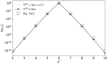
Figure 4: Example of approximate for spherical-spheroidal inner-products $\sigma_{\ell^{\prime}\ell}$ (Eq. 98) for Kerr with dimensionless spin $a=0.01$ and $\ell=6$. Curves compare exact results for the full and approximate spheroidal potentials, $V^{(\mathrm{S})}=-2su+u^{2}\gamma$ and $V^{(\mathrm{S})}\approx-2su$ respectively. Note that the spheroidal differential equation depends on $\gamma V^{(\mathrm{S})}$ (See e.g. Eq. 100).

They emerge from the last term of Eq. (127), when $\bar{\ell}=\ell\pm 1$ and ${\bar{\ell}m}=\ell\pm 2$,

$$\sigma^{(2)}_{\ell\pm 2,\ell}\;=\;\sigma^{(1)}_{\ell\pm 1,\ell}\,\frac{V^{(\mathrm{S})}_{\ell\pm 2,\ell\pm 1}}{E_{\ell\pm 2}-E_{\ell}}\;.$$ (128)

Subsequent orders follow this pattern, with the leading order behavior of each $\sigma_{\ell\pm p,\ell}$ inner product obeying the straight-forward generalization of Eq. (128),

$$\sigma^{(p)}_{\ell\pm p,\ell}\;=\;\sigma^{(p-1)}_{\ell\pm(p-1),\ell}\,\frac{V^{(\mathrm{S})}_{\ell\pm p,\ell\pm(p-1)}}{E_{\ell\pm p}-E_{\ell}}\;.$$ (129)

In Eq. (129), we note the appearance of the absolute difference between $\ell$ and $\bar{\ell}$, namely,

$$p\;=\;|\bar{\ell}-\ell|\;.$$ (130)

With Eq. (129), we have arrived at a recursive formula that is almost ready to lend qualitative insight into the behavior of the spherical-spheroidal inner-products, $\sigma_{\bar{\ell}{{\ell}}}$.

To go further, we may consider the large $p$ behavior of $V_{\ell\pm n,\ell\pm(p-1)}$. It is also useful to recall that the spherical harmonic eigenvalue is

$$E_{\ell m}\;=\;(\ell-s)(\ell+s+1)\;.$$ (131)

Thus, the Clebsh-Gordan coefficients (Eq. 125) along with Eq. (131) communicate that

$$V^{(\mathrm{S})}_{\ell\pm p,\ell\pm(p-1)}\; \sim\;-2\gamma s\,\left(\frac{1}{2}+\mathcal{O}({1}/{p^{2}})\,\right)\;,$$ (132)

$$E_{\ell\pm p,m}-E_{\ell m}\; =\;p\,(1+2\ell+p)\;.$$ (133)

Applying Eqs. (132-133) to the recursion relation presented in Eq. (128) yields

$$\sigma^{(p)}_{\ell\pm p,\ell}\;\approx\;\frac{-\gamma s}{p\,(1+2\ell+p)}\,\sigma^{(p-1)}_{\ell\pm(p-1),\ell}\;.$$ (134)

Equation (128) is the recursive formula for a series whose boundary condition is given by the zeroth order correction, $\sigma^{(0)}_{\ell\ell}=1$. In Eq. (134) we have used Eq. (132) as it is qualitatively accurate for $p>1$. Recursive evaluation of Eq. (134) yields the rather factorial heavy

$$\sigma^{(p)}_{\ell\pm p,\ell}\;\approx\;\left(-\gamma s\right)^{\,p}\;\frac{(2\ell+1)!}{p!(p+2\ell+1)!}\;.$$ (135)

A somewhat simpler but more approximate picture emerges for large $\ell$,

$$\ell\gg p\gg 1$$ (136)

whence we may think of Eq. (134)’s denominator as

$$E_{\ell\pm p,m}-E_{\ell m}\; \approx\;2\ell p\;.$$ (137)

From this perspective the iterative solution to Eq. (134) becomes

$$\sigma^{(p)}_{\ell\pm p,\ell}\;\approx\;\frac{1}{p!}\;\left(\frac{-\gamma s}{2\ell}\right)^{\,p}\;.$$ (138)

In Eq. (138), we have nearly arrived at our destination. Although it was derived under a large $\ell$ assumption, it is qualitatively accurate for $\ell\geq|m|$.

To finish our proof, we need only note that Eq. (135) pertains to the leading order perturbative contribution, $\sigma^{(p)}_{\ell\pm p,\ell}$, rather than the full quantity $\sigma_{\ell\pm p,\ell}$ only as a matter of asymptotics. The full quantity, $\sigma_{\ell\pm p,\ell}$, is equal to $\sigma^{(p)}_{\ell\pm p,\ell}$ plus subdominant higher order terms. But as we are only interested in the leading order approximation, Eq. (135) is equivalent to our prompt, Eq. (98).

Figure 4 presents an example of Eq. (98) applied to Kerr with $a=0.01$. There, the assumption that $V^{(\mathrm{S})}\approx-2su$ and the final approximation (Eq. 98) are compared to the exact numerical calculation. Good agreement is shown.

Appendix B Revisiting the issue of many operators: Physical Spheroidal Harmonics as Eigenfunctions of a Single Operator

The structure of the spherical-spheroidal map ${\mathcal{T}}$ and the existence of the physical adjoint spheroidal harmonics imply and intriguing possibility: we should now be able to construct a single operator for which all of the physical spheroidal harmonics are eigenfunctions. In turn, this raises the possibility that there may be an operator of which the physical adjoint spheroidal harmonics are eigenfunctions. We explore these possibilities in this section. Along the way we encounter a so-called “inter-winding” relationship indicative of two operators which share eigenvalues Shah and Whiting (2016); Rosas-Ortiz and Zelaya (2018); Andrianov et al. (1984).

B.0.1 A unified operator for the physical spheroidal harmonics

In the presence of spacetime angular momentum, a spacetime’s natural modes are spheroidal in nature. The physical spheroidal harmonics naturally emerge in this context. Unlike the fixed oblateness harmonics discussed previously, the physical spheroidal harmonics must be solved simultaneously with a spheroidal radial equation, and as a result have oblatenesses proportional to the polar index, $\ell$ Yang et al. (2012). Although the physical spheroidal harmonics are considered to be a single set of functions, each of these functions has typically been considered to be the eigenfunction of a distinct spheroidal harmonics operator, $\mathcal{L}_{{{{\ell mn}}}}$. This is the operator presented in Eq. (9), and duplicated below for convenience,

$$\mathcal{L}_{{{{\ell mn}}}}=\left(s(1-s)+(u\gamma_{{{{\ell mn}}}}-s)^{2}-\frac{(m+su)^{2}}{1-u^{2}}\right)+\partial_{u}(1-u^{2})\partial_{u}\;.$$ (139)

Here, we are motivated by the possibility that bi-orthogonality in such systems is consistent with the existence of a single operator for which all physical spheroidal harmonics are eigenfunctions. Further, we are motivated by the possibility that this implies the existence of a single such operator for the physical adjoint harmonics, as well as individual operators $\tilde{\mathcal{L}}_{{{\ell mn}}}$ for which each $|{\tilde{S}_{{{\ell mn}}}}\rangle$ is an eigenfunction.

To this end, we start by noting that the physical spherical-spheroidal map ${\mathcal{T}}$ (Eq. 53) already has the key properties of such an operator: when acting on select functions with label ${{{\ell mn}}}$, it has the effect of a ${{{\ell mn}}}$-specific operator. With this in mind, we seek an operator $\mathcal{L}$, such that

$$\mathcal{L}\,|{S_{{{\ell mn}}}}\rangle\;=\;\mathcal{L}_{{{{\ell mn}}}}\,|{S_{k}}\rangle\;=\;-A_{{{\ell mn}}}\,|{S_{{{\ell mn}}}}\rangle\;\text{for all}\;{{{\ell mn}}}.$$ (140)

With this in mind, the structure of ${\mathcal{T}}$ and the existence of the physical adjoint-harmonics allow for $\mathcal{L}$ of the form,

$$\mathcal{L}\; =\;\sum_{{{\ell^{\prime}}}}^{\infty}\,\mathcal{L}_{{{\ell^{\prime}mn}}}\,|{S_{{{\ell^{\prime}mn}}}}\rangle\langle{\tilde{S}_{{{\ell^{\prime}mn}}}}|\;$$ (141)

$$=\;\sum_{{{\ell^{\prime}}}}^{\infty}\,-A_{{{\ell^{\prime}mn}}}\,|{S_{{{\ell^{\prime}mn}}}}\rangle\langle{\tilde{S}_{{{\ell^{\prime}mn}}}}|\;.$$ (142)

Equation (141) is required for Eq. (140) to hold, and Eq. (142) is simply the matrix representation of $\mathcal{L}$ in the bases of spheroidal harmonics (rows) and adjoint spheroidals (columns). In this way the existence of the adjoint spheroidal harmonics enables the physical spheroidals to be unified under a single operator, $\mathcal{L}$.

B.0.2 An operator for the physical adjoint spheroidal harmonics

We are now interested in whether an analog of the spheroidal harmonic differential equation $\mathcal{L}_{{{{\ell mn}}}}$ (Eq. 139) may be constructed for the physical adjoint harmonics. Such an operator should be manifestly consistent with the bi-orthogonality between the spheroidal harmonics and their adjoints. Recalling our discussion of the fixed oblateness spheroidals, it is clear that the adjoint spheroidal harmonics must be eigenfunctions of ${\mathcal{L}}$’s adjoint,

$${\mathcal{L}}^{\dagger}\; =\;\sum_{{{\ell^{\prime}}}}\,|{\tilde{S}_{{{\ell^{\prime}mn}}}}\rangle\langle{S_{{{\ell^{\prime}mn}}}}|\,{\mathcal{L}}^{\dagger}_{{{\ell^{\prime}mn}}}\;$$ (143)

$$=\;\sum_{{{\ell^{\prime}}}}\,-A^{*}_{{{\ell^{\prime}mn}}}\,|{\tilde{S}_{{{\ell^{\prime}mn}}}}\rangle\langle{S_{{{\ell^{\prime}mn}}}}|\;.$$ (144)

Equations (143-144) generalize the same relationship for the fixed oblateness harmonics presented during our discussion of the adjoint eigenfunctions under fixed oblateness (Eq. 9). In Eq. (143), we have used that fact adjugating a product of operators reverses ordering Lax (2002); Christensen (2003). In Eq. (144), we have simply adjugated the last statement of Eq. (141).

Interestingly, Eq. (143) communicates that, if there exist operators $\tilde{\mathcal{L}}_{{{\ell mn}}}$ such that $|{\tilde{S}_{{{\ell mn}}}}\rangle$ are eigenfunctions, then

$$\sum_{{{\ell^{\prime}}}}\,\tilde{\mathcal{L}}_{{{\ell^{\prime}mn}}}\,|{\tilde{S}_{{{\ell^{\prime}mn}}}}\rangle\langle{S_{{{\ell^{\prime}mn}}}}|\;=\;\sum_{{{\ell^{\prime}}}}\,|{\tilde{S}_{{{\ell^{\prime}mn}}}}\rangle\langle{S_{{{\ell^{\prime}mn}}}}|\,{\mathcal{L}}^{\dagger}_{{{\ell^{\prime}mn}}}\;,$$ (145)

with

$$\tilde{\mathcal{L}}_{{{\ell^{\prime}mn}}}\,|{\tilde{S}_{{{\ell^{\prime}mn}}}}\rangle\;=\;-A_{{{\ell^{\prime}mn}}}^{*}\,|{\tilde{S}_{{{\ell^{\prime}mn}}}}\rangle\;.$$ (146)

Perhaps uninterestingly, Eq. (146) is the generalization of the adjoint eigenvalue relation for the fixed oblateness harmonics (Eq. 13). Equation (145) is perhaps more interesting: applying $\langle{S_{{{\ell mn}}}}|$ on the left and $|{\tilde{S}_{{{\ell mn}}}}\rangle$ on the right allows the extraction of terms

$$\sum_{{{\ell^{\prime}}}}\langle{S_{{{\ell mn}}}}|\tilde{\mathcal{L}}_{{{\ell^{\prime}mn}}}|{\tilde{S}_{{{\ell^{\prime}mn}}}}\rangle{\langle{S_{{{\ell^{\prime}mn}}}}\,|\,{\tilde{S}_{{{\ell mn}}}}\rangle} =\sum_{{{\ell^{\prime}}}}{\langle{S_{{{\ell mn}}}}\,|\,{\tilde{S}_{{{\ell^{\prime}mn}}}}\rangle}\langle{S_{{{\ell^{\prime}mn}}}}|{\mathcal{L}}^{\dagger}_{{{\ell^{\prime}mn}}}|{\tilde{S}_{{{\ell mn}}}}\rangle$$ (147)

$$\sum_{{{\ell^{\prime}}}}{\langle{S_{{{\ell mn}}}}\,|\,{\tilde{\mathcal{L}}_{{{\ell^{\prime}mn}}}\tilde{S}_{{{\ell^{\prime}mn}}}}\rangle}{\langle{S_{{{\ell^{\prime}mn}}}}\,|\,{\tilde{S}_{{{\ell mn}}}}\rangle} =\sum_{{{\ell^{\prime}}}}{\langle{S_{{{\ell mn}}}}\,|\,{\tilde{S}_{{{\ell^{\prime}mn}}}}\rangle}{\langle{{\mathcal{L}}_{{{\ell^{\prime}mn}}}S_{{{\ell^{\prime}mn}}}}\,|\,{\tilde{S}_{{{\ell mn}}}}\rangle}$$ (148)

$${\langle{S_{{{\ell mn}}}}\,|\,{\tilde{\mathcal{L}}_{{{\ell mn}}}\tilde{S}_{{{\ell mn}}}}\rangle}\; =\;{\langle{{\mathcal{L}}_{{{\ell mn}}}S_{{{\ell mn}}}}\,|\,{\tilde{S}_{{{\ell mn}}}}\rangle}\;.$$ (149)

In Eqs. (147-149) we have taken care to render the connection between $\mathcal{L}_{{{\ell mn}}}$ and $\tilde{\mathcal{L}}_{{{\ell mn}}}$, as it may not be immediately clear from Eqs. (145-146). In going from Eq. (147) to Eq. (148) we have grouped operators with harmonics that have the same label. In Eq. (148)’s right-hand side, we have used the defining property of the adjoint operator (Eq. 11). In Eq. (149) we have applied bi-orthogonality (Eq. 38).

Together, Eqs. (140-149) illustrate the required relationships between $\mathcal{L}_{{{\ell mn}}}$ and $\tilde{\mathcal{L}}_{{{\ell mn}}}$. Equation (140) and Eq. (146) communicate that $\tilde{\mathcal{L}}_{{{\ell mn}}}$ has the same eigenvalues as $\mathcal{L}_{{{\ell mn}}}^{*}$ , and by Eq. (12) we recall that

$${\mathcal{L}}^{\dagger}_{{{\ell mn}}}=\mathcal{L}^{*}_{{{\ell mn}}}\;.$$ (150)

In this sense, we say that $\tilde{\mathcal{L}}_{{{\ell mn}}}$ is isospectral with ${\mathcal{L}}^{\dagger}_{{{\ell mn}}}$ Mostafazadeh (2002); Rosas-Ortiz and Zelaya (2018). Finally, Eq. (149) communicates that in the case of fixed oblateness, $\tilde{\mathcal{L}}_{{{\ell mn}}}$ would simply be the adjoint of $\mathcal{L}_{{{\ell mn}}}$.

The condition of isospectrality is most interesting. Two operators are isospectral if there exists an operator, $\mathcal{P}$, with inverse $\mathcal{Q}$, such that

$$\mathcal{P}\,{\mathcal{L}}^{\dagger}_{{{\ell mn}}}\; =\;\tilde{\mathcal{L}}_{{{\ell mn}}}\,\mathcal{P}$$ (151)

$${\mathcal{L}}^{\dagger}_{{{\ell mn}}}\,\mathcal{Q}\; =\;\mathcal{Q}\,\tilde{\mathcal{L}}_{{{\ell mn}}}\;,$$ (152)

or, equivalently, since ${\mathcal{L}}^{\dagger}_{{{\ell mn}}}=\mathcal{L}^{*}_{{{\ell mn}}}$,

$$\tilde{\mathcal{L}}_{{{\ell mn}}}\;=\;\mathcal{P}\,{\mathcal{L}^{*}}_{{{\ell mn}}}\,\mathcal{Q}\;.$$ (153)

Equation (151) presents what are called inter-winding relationships Andrianov et al. (1984); Rosas-Ortiz and Zelaya (2018). Equation (153) communicates that, given $\mathcal{P}$ and $\mathcal{Q}$, we may transform ${\mathcal{L}^{*}}_{{{\ell mn}}}$ into $\tilde{\mathcal{L}}_{{{\ell mn}}}$.

The use of Eqs. (151-152) is that they relate eigenfunctions of ${\mathcal{L}^{*}}_{{{\ell mn}}}$ to those of $\tilde{\mathcal{L}}_{{{\ell mn}}}$. For example, applying $|{S_{{{\ell mn}}}^{*}}\rangle$ on the left of Eq. (151) gives

$$\tilde{\mathcal{L}}_{{{\ell mn}}}\,\mathcal{P}\,|{S^{*}_{{{\ell mn}}}}\rangle\; =\;\mathcal{P}\,{\mathcal{L}^{*}}_{{{\ell mn}}}\,|{S^{*}_{{{\ell mn}}}}\rangle$$ (154)

$$\tilde{\mathcal{L}}_{{{\ell mn}}}\,\mathcal{P}\,|{S^{*}_{{{\ell mn}}}}\rangle\; =\;-A^{*}_{{{\ell mn}}}\,\mathcal{P}\,|{S^{*}_{{{\ell mn}}}}\rangle\;.$$ (155)

In going from Eq. (154) to Eq. (155), we apply the eigenvalue relationship appropriate for the conjugate harmonics (Eq. 13). Equation (155) communicates that $\mathcal{P}\,|{S^{*}_{{{\ell mn}}}}\rangle$ is an eigenfunction of $\tilde{\mathcal{L}}_{{{\ell mn}}}$, and so $\mathcal{P}\,|{S^{*}_{{{\ell mn}}}}\rangle$ must be an adjoint-spheroidal function. Thus $\mathcal{P}$ maps conjugated spheroidal harmonics to physical adjoint harmonics, and $\mathcal{Q}$ must have the opposite effect

$$|{\tilde{S}_{{{\ell mn}}}}\rangle\;=\;\mathcal{P}\,|{S^{*}_{{{\ell mn}}}}\rangle\;,$$ (156)

$$|{S^{*}_{{{\ell mn}}}}\rangle\;=\;\mathcal{Q}\,|{\tilde{S}_{{{\ell mn}}}}\rangle\;.$$ (157)

Like ${\mathcal{T}}$, which uses bi-orthogonality to map spherical harmonics into spheroidals, we may write $\mathcal{P}$ and $\mathcal{Q}$ as a sum over projectors

$$\mathcal{P}\;=\;\sum_{{{\ell^{\prime}}}}\,|{\tilde{S}_{{{\ell^{\prime}mn}}}}\rangle\langle{\tilde{S}^{*}_{{{\ell^{\prime}mn}}}}|\;,$$ (158)

$$\mathcal{Q}\;=\;\sum_{{{\ell^{\prime}}}}\,|{S^{*}_{{{\ell^{\prime}mn}}}}\rangle\langle{S_{{{\ell^{\prime}mn}}}}|\;.$$ (159)

In Eq. (158) we have noted and made use of the fact that the complex conjugates of the physical spheroidals and their adjoints are also bi-orthogonal,

$${\langle{\tilde{S}^{*}_{{{\ell^{\prime}mn}}}}\,|\,{S^{*}_{{{\ell mn}}}}\rangle}\;=\;{\langle{\tilde{S}_{{{\ell^{\prime}mn}}}}\,|\,{S_{{{\ell mn}}}}\rangle}^{*}\;=\;\delta_{{{\ell^{\prime}}}{{\ell}}}\;.$$ (160)

Using Eq. (160) it may be easily verified that the $\mathcal{P}$ and $\mathcal{Q}$ of Eq. (158) have the properties given in Eqs. (156-157). Together, Eq. (153) and Eq. (158) allow $\tilde{\mathcal{L}}_{{{\ell mn}}}$ to be written as

$$\tilde{\mathcal{L}}_{{{\ell mn}}}\;=\;\sum_{{{\ell^{\prime}}},{{\ell}}^{\prime\prime}}\,|{\tilde{S}_{{{\ell^{\prime}mn}}}}\rangle\langle{\tilde{S}^{*}_{{{\ell^{\prime}mn}}}}|\,{\mathcal{L}^{*}}_{{{\ell mn}}}\,|{S^{*}_{{{\ell}}^{\prime\prime}mn}}\rangle\langle{S_{{{\ell}}^{\prime\prime}mn}}|\;.$$ (161)

Equation (161) presents a matrix representation for $\tilde{\mathcal{L}}_{{{\ell mn}}}$, the operator for which the adjoint-spherical harmonics are eigenfunctions. It is fair to think of $\tilde{\mathcal{L}}_{{{\ell mn}}}$ as a “heterogeneous adjoint”, as Eq. (161) communicates that it relies on multiple physical oblatenesses rather than one. It may be of future interest to determine whether $\tilde{\mathcal{L}}_{{{\ell mn}}}$ has a linear differential form that does not require prior knowledge of its eigenfunctions.

References

- Abbott et al. (2019) B. Abbott et al. (LIGO Scientific, Virgo), Phys. Rev. X 9, 031040 (2019), arXiv:1811.12907 [astro-ph.HE] .
- Abbott et al. (2020) R. Abbott et al. (LIGO Scientific, Virgo), (2020), arXiv:2004.08342 [astro-ph.HE] .
- Teukolsky (1973) S. A. Teukolsky, Astrophys. J. 185, 635 (1973).
- Newman and Penrose (1966) E. T. Newman and R. Penrose, Journal of Mathematical Physics 7, 863 (1966), https://doi.org/10.1063/1.1931221 .
- Thorne (1980) K. S. Thorne, Rev. Mod. Phys. 52, 299 (1980).
- Ruiz et al. (2008) M. Ruiz, R. Takahashi, M. Alcubierre, and D. Nunez, Gen. Rel. Grav. 40, 2467 (2008), arXiv:0707.4654 [gr-qc] .
- Breuer et al. (1977) R. A. Breuer, M. P. Ryan, Jr., and S. Waller, Proceedings of the Royal Society of London Series A 358, 71 (1977).
- London et al. (2014) L. London, D. Shoemaker, and J. Healy, Phys. Rev. D90, 124032 (2014), arXiv:1404.3197 [gr-qc] .
- Leaver (1985) E. Leaver, Proc. Roy. Soc. Lond. A A402, 285 (1985).
- Hughes (2000) S. A. Hughes, Phys. Rev. D 61, 084004 (2000), [Erratum: Phys.Rev.D 63, 049902 (2001), Erratum: Phys.Rev.D 65, 069902 (2002), Erratum: Phys.Rev.D 67, 089901 (2003), Erratum: Phys.Rev.D 78, 109902 (2008), Erratum: Phys.Rev.D 90, 109904 (2014)], arXiv:gr-qc/9910091 .
- London et al. (2018) L. London, S. Khan, E. Fauchon-Jones, C. García, M. Hannam, S. Husa, X. Jiménez-Forteza, C. Kalaghatgi, F. Ohme, and F. Pannarale, Phys. Rev. Lett. 120, 161102 (2018), arXiv:1708.00404 [gr-qc] .
- Holzegel and Smulevici (2013) G. Holzegel and J. Smulevici, (2013), 10.2140/apde.2014.7.1057, arXiv:1303.5944 [gr-qc] .
- Berti et al. (2006a) E. Berti, V. Cardoso, and M. Casals, Phys. Rev. D73, 024013 (2006a), [Erratum: Phys. Rev.D73,109902(2006)], arXiv:gr-qc/0511111 [gr-qc] .
- Berti and Klein (2014) E. Berti and A. Klein, Phys. Rev. D 90, 064012 (2014), arXiv:1408.1860 [gr-qc] .
- Kelly and Baker (2013) B. J. Kelly and J. G. Baker, Phys. Rev. D 87, 084004 (2013), arXiv:1212.5553 [gr-qc] .
- García-Quirós et al. (2020) C. García-Quirós, M. Colleoni, S. Husa, H. Estellés, G. Pratten, A. Ramos-Buades, M. Mateu-Lucena, and R. Jaume, (2020), arXiv:2001.10914 [gr-qc] .
- Blackman et al. (2017) J. Blackman, S. E. Field, M. A. Scheel, C. R. Galley, C. D. Ott, M. Boyle, L. E. Kidder, H. P. Pfeiffer, and B. Szilágyi, Phys. Rev. D 96, 024058 (2017), arXiv:1705.07089 [gr-qc] .
- Mehta et al. (2019) A. K. Mehta, P. Tiwari, N. K. Johnson-McDaniel, C. K. Mishra, V. Varma, and P. Ajith, Phys. Rev. D100, 024032 (2019), arXiv:1902.02731 [gr-qc] .
- Carullo et al. (2018) G. Carullo et al., Phys. Rev. D 98, 104020 (2018), arXiv:1805.04760 [gr-qc] .
- Ghosh et al. (2016) A. Ghosh et al., Phys. Rev. D94, 021101 (2016), arXiv:1602.02453 [gr-qc] .
- Ota and Chirenti (2020) I. Ota and C. Chirenti, Phys. Rev. D 101, 104005 (2020), arXiv:1911.00440 [gr-qc] .
- Bhagwat et al. (2020) S. Bhagwat, X. J. Forteza, P. Pani, and V. Ferrari, Phys. Rev. D 101, 044033 (2020), arXiv:1910.08708 [gr-qc] .
- Mino et al. (1997) Y. Mino, M. Sasaki, M. Shibata, H. Tagoshi, and T. Tanaka, Progress of Theoretical Physics Supplement 128, 1 (1997), http://oup.prod.sis.lan/ptps/article-pdf/doi/10.1143/PTPS.128.1/5438984/128-1.pdf .
- O’Sullivan and Hughes (2014) S. O’Sullivan and S. A. Hughes, Phys. Rev. D 90, 124039 (2014), [Erratum: Phys.Rev.D 91, 109901 (2015)], arXiv:1407.6983 [gr-qc] .
- Blanchet (2014) L. Blanchet, Living Rev. Rel. 17, 2 (2014), arXiv:1310.1528 [gr-qc] .
- London (2021) L. London, “Bi-orthogonal harmonics for the decomposition of gravitational radiation II: applications for extreme and comparable mass-ratio black hole binaries (Submittted to PRL),” (2021).
- Brauer (1964) F. Brauer, Michigan Math. J. 11, 379 (1964).
- Christensen (2003) O. Christensen, An Introduction to Frames and Riesz Bases (Birkhäuser Boston, 2003).
- Green et al. (2022) S. Green et al., “In preparation.” (2022).
- Sberna et al. (2022) L. Sberna, P. Bosch, W. E. East, S. R. Green, and L. Lehner, Phys. Rev. D 105, 064046 (2022), arXiv:2112.11168 [gr-qc] .
- London et al. (2020) L. London, E. Fauchon, and E. Hamilton, “llondon6/positive: map,” (2020).
- Courant and Hilbert. (1954) R. Courant and D. Hilbert., Quarterly Journal of the Royal Meteorological Society 80, 485 (1954).
- Berti et al. (2006b) E. Berti, V. Cardoso, and C. M. Will, Phys. Rev. D73, 064030 (2006b), arXiv:gr-qc/0512160 [gr-qc] .
- Nollert (1999) H.-P. Nollert, Class. Quant. Grav. 16, R159 (1999).
- Andersson (1997) N. Andersson, Phys. Rev. D 55, 468 (1997), arXiv:gr-qc/9607064 .
- Bhagwat et al. (2017) S. Bhagwat, M. Okounkova, S. W. Ballmer, D. A. Brown, M. Giesler, M. A. Scheel, and S. A. Teukolsky, (2017), arXiv:1711.00926 [gr-qc] .
- Mostafazadeh (2002) A. Mostafazadeh, J. Math. Phys. 43, 205 (2002), arXiv:math-ph/0107001 .
- Shah and Whiting (2016) A. G. Shah and B. F. Whiting, Gen. Rel. Grav. 48, 78 (2016), arXiv:1503.02618 [gr-qc] .
- Cook and Zalutskiy (2014) G. B. Cook and M. Zalutskiy, Phys. Rev. D 90, 124021 (2014), arXiv:1410.7698 [gr-qc] .
- London and Fauchon-Jones (2019) L. London and E. Fauchon-Jones, Class. Quant. Grav. 36, 235015 (2019), arXiv:1810.03550 [gr-qc] .
- Magaña Zertuche et al. (2021) L. Magaña Zertuche et al., (2021), arXiv:2110.15922 [gr-qc] .
- Kamaretsos et al. (2012a) I. Kamaretsos, M. Hannam, S. Husa, and B. Sathyaprakash, Phys.Rev. D85, 024018 (2012a), arXiv:1107.0854 [gr-qc] .
- Husa et al. (2016) S. Husa, S. Khan, M. Hannam, M. Pürrer, F. Ohme, X. Jiménez Forteza, and A. Bohé, Phys. Rev. D93, 044006 (2016), arXiv:1508.07250 [gr-qc] .
- Khan et al. (2016) S. Khan, S. Husa, M. Hannam, F. Ohme, M. Pürrer, X. Jiménez Forteza, and A. Bohé, Phys. Rev. D93, 044007 (2016), arXiv:1508.07253 [gr-qc] .
- Hamilton et al. (2021) E. Hamilton, L. London, J. E. Thompson, E. Fauchon-Jones, M. Hannam, C. Kalaghatgi, S. Khan, F. Pannarale, and A. Vano-Vinuales, (2021), arXiv:2107.08876 [gr-qc] .
- Berti et al. (2016) E. Berti, A. Sesana, E. Barausse, V. Cardoso, and K. Belczynski, Phys. Rev. Lett. 117, 101102 (2016), arXiv:1605.09286 [gr-qc] .
- Kamaretsos et al. (2012b) I. Kamaretsos, M. Hannam, and B. Sathyaprakash, Phys.Rev.Lett. 109, 141102 (2012b), arXiv:1207.0399 [gr-qc] .
- Keitel et al. (2017) D. Keitel et al., Phys. Rev. D96, 024006 (2017), arXiv:1612.09566 [gr-qc] .
- Jaramillo et al. (2020) J. L. Jaramillo, R. Panosso Macedo, and L. Al Sheikh, (2020), arXiv:2004.06434 [gr-qc] .
- Axler (2015) S. Axler, Linear algebra done right (Springer, Cham, 2015).
- Seidel (1989) E. Seidel, Class. Quant. Grav. 6, 1057 (1989).
- Press and Teukolsky (1973) W. H. Press and S. A. Teukolsky, Astrophys. J. 185, 649 (1973).
- Yang et al. (2012) H. Yang, D. A. Nichols, F. Zhang, A. Zimmerman, Z. Zhang, and Y. Chen, Phys. Rev. D 86, 104006 (2012), arXiv:1207.4253 [gr-qc] .
- Cotesta et al. (2018) R. Cotesta, A. Buonanno, A. Bohé, A. Taracchini, I. Hinder, and S. Ossokine, Phys. Rev. D 98, 084028 (2018), arXiv:1803.10701 [gr-qc] .
- Hughes et al. (2019) S. A. Hughes, A. Apte, G. Khanna, and H. Lim, Phys. Rev. Lett. 123, 161101 (2019), arXiv:1901.05900 [gr-qc] .
- London (2020) L. London, “Modeling ringdown. II. Aligned-spin binary black holes, implications for data analysis and fundamental theory,” (2020), arXiv:1801.08208 [gr-qc] .
- Le Tiec et al. (2010) A. Le Tiec, L. Blanchet, and C. M. Will, Class. Quant. Grav. 27, 012001 (2010), arXiv:0910.4594 [gr-qc] .
- Ossokine et al. (2020) S. Ossokine et al., Phys. Rev. D 102, 044055 (2020), arXiv:2004.09442 [gr-qc] .
- Giesler et al. (2019) M. Giesler, M. Isi, M. A. Scheel, and S. Teukolsky, Phys. Rev. X 9, 041060 (2019), arXiv:1903.08284 [gr-qc] .
- Abbott et al. (2021) R. Abbott et al. (LIGO Scientific, Virgo), Phys. Rev. X 11, 021053 (2021), arXiv:2010.14527 [gr-qc] .
- Rosas-Ortiz and Zelaya (2018) O. Rosas-Ortiz and K. Zelaya, Annals of Physics 388, 26 (2018).
- Andrianov et al. (1984) A. Andrianov, N. Borisov, and M. V. Ioffe, Theor. Math. Phys. 61, 1078 (1984).
- Lax (2002) P. Lax, Functional analysis (Wiley, New York, 2002).