A note on Almgren-Chriss optimal execution problem with geometric Brownian motion111The ideas presented in this paper do not necessarily reflect the views or practices at Ritter Alpha LP. This work benefits from the financial support of the Chaires Analytics and Models for Regulation, Financial Risk and Finance and Sustainable Development. Bastien Baldacci gratefully acknowledge the financial support of the ERC Grant 679836 Staqamof. The authors would like to thank Robert Almgren, Peter Carr, Jim Gatheral, Dylan Possamai and Mathieu Rosenbaum for fruitful discussions. In particular, Peter Carr deserves warm thanks as this article would not exist without his inputs.

Bastien Baldacci
CMAP, Ecole Polytechnique
bastien.baldacci@polytechnique.edu
   Jerome Benveniste
Ritter Alpha LP and NYU
ejb14@nyu.edu
Abstract

We solve explicitly the Almgren-Chriss optimal liquidation problem where the stock price process follows a geometric Brownian motion. Our technique is to work in terms of cash and to use functional analysis tools. We show that this framework extends readily to the case of a stochastic drift for the price process and the liquidation of a portfolio.

Keywords: Almgren-Chriss, optimal liquidation, adjoint operator.

1 Introduction

Optimal liquidation is a problem faced by a trader when he needs to liquidate a large number of shares. The trader faces a tradeoff between fast execution, reducing a risk related to price changes and slow execution, allowing to avoid high trading costs. Since the seminal paper by Almgren and Chriss [2], various extensions of optimal liquidation problems have been studied, see for example  [1, 3, 8]. The common framework to address this issue introduced in [2] assumes the following:

  • the efficient price process follows an arithmetic Brownian motion (ABM),

  • permanent market impact is linear,

  • transaction costs are a linear function of the trading rate.

The execution of a large order is then formulated in discrete time as a tradeoff between expected costs and risk of the trading strategy, with variance as a risk measure. Under this framework, there exists a unique optimal liquidation strategy, which is a deterministic function of time and the initial position of the trader.

Continuous versions of this problem have been considered, notably in [5, 6], where the author shows the ill-posedness of the mean-variance framework leading to time-inconsistent solutions. To overcome this issue, the authors suggest using alternative objective functions, particularly mean-quadratic variation. Under this choice, the authors solve a two-dimensional Hamilton-Jacobi-Bellman equation numerically. Moreover, in [8], the authors consider the optimal execution problem with CARA utility objective function. To the best of our knowledge, there is no closed-form solution to the continuous version of the Almgren-Chriss framework with quadratic variation as a risk measure and geometric Brownian motion (GBM) assumption for the efficient price process. In [7], the authors solve a modified version of the problem with GBM, accounting for the risk with a linear function of the trading rate.

In this paper, we solve the optimal liquidation problem under the Almgren-Chriss framework in continuous time, in the case where the efficient price process follows a GBM, and the risk measure is quadratic variation. Motivated by [4], we assume that trading costs are a quadratic function of the amount of cash, instead of shares. Thus, we reformulate the problem in terms of cash traded and derive in closed-form the optimal control of the trader liquidating his position. As the method is based on the resolution of a system of ODEs, it does not suffer from the curse of dimensionality. In particular, we show how to extend this framework to the case of the liquidation of a portfolio of N𝑁N, possibly correlated, assets. It also enables us to treat the case where the return’s drift is a stochastic process without any BSDE methods with a singular condition.

The paper is organized as follows. In Section 2, we describe the Almgren Chriss framework in continuous time and reformulate the optimization problem in terms of cash. In Section 3, we obtain a closed-form solution of the Almgren Chriss framework with GBM for the efficient price process. Finally in Section 4, we present numerical applications under different market conditions.

2 The model

We define (Ω,t[0,T],)Ωsubscript𝑡0𝑇(\Omega,\mathcal{F}_{t\in[0,T]},\mathbb{P}) a filtered probability space, on which all stochastic process are defined, and a trading horizon is T>0𝑇0T>0.

2.1 Almgren-Chriss framework in continuous time

We rapidly recall the well-known Almgren-Chriss problem in continuous time. We consider the issue of the liquidation of q0subscript𝑞0q_{0}\in\mathbb{R} shares of a stock whose price at time t𝑡t is defined by Stsubscript𝑆𝑡S_{t}. The number of shares hold by the trader is defined by an absolutely continuous measurable process qt:=q00tq.sdsassignsubscript𝑞𝑡subscript𝑞0superscriptsubscript0𝑡subscript.𝑞𝑠differential-d𝑠q_{t}:=q_{0}-\int_{0}^{t}\overset{.}{q}_{s}\mathrm{d}s where (q.s)s[0,T]subscriptsubscript.𝑞𝑠𝑠0𝑇(\overset{.}{q}_{s})_{s\in[0,T]} is the trading rate, controlled by the trader. The transaction price is

S~t:=St+λ2q.t+γ(qtq0),assignsubscript~𝑆𝑡subscript𝑆𝑡𝜆2subscript.𝑞𝑡𝛾subscript𝑞𝑡subscript𝑞0\displaystyle\tilde{S}_{t}:=S_{t}+\frac{\lambda}{2}\overset{.}{q}_{t}+\gamma(q_{t}-q_{0}),

where λ,γ+𝜆𝛾superscript\lambda,\gamma\in\mathbb{R}^{+} are constants related respectively to temporary and permanent price impact. Indeed, the term λ2q.t𝜆2subscript.𝑞𝑡\frac{\lambda}{2}\overset{.}{q}_{t} is the impact of trading q.tsubscript.𝑞𝑡\overset{.}{q}_{t} shares at time t𝑡t, whereas the term γ(qtq0)𝛾subscript𝑞𝑡subscript𝑞0\gamma(q_{t}-q_{0}) is the impact generated by the flow of transactions up to time t𝑡t. In the original framework in discrete time, see [2], and in most of the extensions in continuous time, see [8] for example, the price process follows an ABM. The number of shares hold by the trader satisfies the boundary condition qT=0subscript𝑞𝑇0q_{T}=0. Therefore, the cost of this strategy during the trading period is

𝒞(q.):=0TS~tqtdt.assign𝒞.𝑞superscriptsubscript0𝑇subscript~𝑆𝑡subscript𝑞𝑡differential-d𝑡\displaystyle\mathcal{C}(\overset{.}{q}):=\int_{0}^{T}\tilde{S}_{t}q_{t}\mathrm{d}t.

Aiming at remedying the time inconsistency of the optimal strategies in the pre-commitment mean-variance framework, inspired by [6], we replace the variance by the quadratic variation in the penalty. The optimal execution problem consists in the optimization of a mean-quadratic variation objective function over the strategies (q.t)t[0,T]𝒜subscriptsubscript.𝑞𝑡𝑡0𝑇𝒜(\overset{.}{q}_{t})_{t\in[0,T]}\in\mathcal{A} where

𝒜:={(q.t)t[0,T],tmeasurable such that 0Tq.s𝑑s=q0}.assign𝒜subscriptsubscript.𝑞𝑡𝑡0𝑇subscript𝑡measurable such that superscriptsubscript0𝑇subscript.𝑞𝑠differential-d𝑠subscript𝑞0\displaystyle\mathcal{A}:=\Big{\{}(\overset{.}{q}_{t})_{t\in[0,T]},\mathcal{F}_{t}-\text{measurable such that }\int_{0}^{T}\overset{.}{q}_{s}ds=q_{0}\Big{\}}.

The problem can be written as follows:

supv𝒜𝔼[𝒞(q.)κ2𝒞T],subscriptsupremum𝑣𝒜𝔼delimited-[]𝒞.𝑞𝜅2subscriptdelimited-⟨⟩𝒞𝑇\displaystyle\sup_{v\in\mathcal{A}}\mathbb{E}\big{[}-\mathcal{C}(\overset{.}{q})-\frac{\kappa}{2}\langle\mathcal{C}\rangle_{T}\big{]},

with κ>0𝜅0\kappa>0 and

𝒞T:=0Tqt2dSt.assignsubscriptdelimited-⟨⟩𝒞𝑇superscriptsubscript0𝑇superscriptsubscript𝑞𝑡2dsubscriptdelimited-⟨⟩𝑆𝑡\displaystyle\langle\mathcal{C}\rangle_{T}:=\int_{0}^{T}q_{t}^{2}\mathrm{d}\langle S\rangle_{t}.

The use of quadratic variation leads to time-consistent strategies. Moreover, in contrast to the variance, quadratic variation takes into account the trajectory of liquidation. A direct integration by parts on 𝒞(q)𝒞𝑞\mathcal{C}(q) gives

𝒞(q)=q0S00TqtdSt+λ20Tq.t2dt+γ2q02.𝒞𝑞subscript𝑞0subscript𝑆0superscriptsubscript0𝑇subscript𝑞𝑡differential-dsubscript𝑆𝑡𝜆2superscriptsubscript0𝑇superscriptsubscript.𝑞𝑡2differential-d𝑡𝛾2superscriptsubscript𝑞02\displaystyle\mathcal{C}(q)=-q_{0}S_{0}-\int_{0}^{T}q_{t}\mathrm{d}S_{t}+\frac{\lambda}{2}\int_{0}^{T}\overset{.}{q}_{t}^{2}\mathrm{d}t+\frac{\gamma}{2}q_{0}^{2}.

Therefore, the problem writes as

supq.𝒜𝔼[0TqtdStλ20Tq.t2dtκ20Tqt2dSt].subscriptsupremum.𝑞𝒜𝔼delimited-[]superscriptsubscript0𝑇subscript𝑞𝑡differential-dsubscript𝑆𝑡𝜆2superscriptsubscript0𝑇superscriptsubscript.𝑞𝑡2differential-d𝑡𝜅2superscriptsubscript0𝑇superscriptsubscript𝑞𝑡2dsubscriptdelimited-⟨⟩𝑆𝑡\displaystyle\sup_{\overset{.}{q}\in\mathcal{A}}\mathbb{E}\Big{[}\int_{0}^{T}q_{t}\mathrm{d}S_{t}-\frac{\lambda}{2}\int_{0}^{T}\overset{.}{q}_{t}^{2}\mathrm{d}t-\frac{\kappa}{2}\int_{0}^{T}q_{t}^{2}\mathrm{d}\langle S\rangle_{t}\Big{]}. (2.1)

When the price process follows an ABM, Problem (2.1) boils down to a simple calculus of variations problem, which has been solved, for example, in [8]. The case where the dynamics are given by a GBM is more intricate. In [7], the authors consider it analytically intractable when a quadratic variation penalty is used. Moreover, in [6], the authors derive a numerical solution of (2.1) by solving the corresponding Hamilton-Jacobi-Bellman equation. Note that strategies under ABM assumption are good proxies of the ones under GBM assumption in period of low volatility.

2.2 Reformulation in terms of cash

We now reformulate the optimal execution problem in terms of cash. We emphasize that we treat the very same problem as in (2.1), except that we modify the transaction costs such that the penalty for q.tsubscript.𝑞𝑡\overset{.}{q}_{t} becomes q.tStsubscript.𝑞𝑡subscript𝑆𝑡\overset{.}{q}_{t}S_{t}.

We assume that the price process follows a GBM:

dSt=σStdWt.dsubscript𝑆𝑡𝜎subscript𝑆𝑡dsubscript𝑊𝑡\displaystyle\mathrm{d}S_{t}=\sigma S_{t}\mathrm{d}W_{t}.

Multiplying above and below by Stsubscript𝑆𝑡S_{t}, we obtain that

0TqtdSt=0Tθtdyt,superscriptsubscript0𝑇subscript𝑞𝑡differential-dsubscript𝑆𝑡superscriptsubscript0𝑇subscript𝜃𝑡differential-dsubscript𝑦𝑡\displaystyle\int_{0}^{T}q_{t}\mathrm{d}S_{t}=\int_{0}^{T}\theta_{t}\mathrm{d}y_{t},

where dyt:=σdWtassigndsubscript𝑦𝑡𝜎dsubscript𝑊𝑡\mathrm{d}y_{t}:=\sigma\mathrm{d}W_{t} is the return of the price process, and θt:=qtStassignsubscript𝜃𝑡subscript𝑞𝑡subscript𝑆𝑡\theta_{t}:=q_{t}S_{t} is the trader’s position expressed in dollars. Moreover, the quadratic variation penalty has the form

κσ220Tθt2dt.𝜅superscript𝜎22superscriptsubscript0𝑇superscriptsubscript𝜃𝑡2differential-d𝑡\displaystyle\frac{\kappa\sigma^{2}}{2}\int_{0}^{T}\theta_{t}^{2}\mathrm{d}t.

Applying Ito’s formula, we derive that the cash position θt:=θtuassignsubscript𝜃𝑡superscriptsubscript𝜃𝑡𝑢\theta_{t}:=\theta_{t}^{u} has the following dynamics:222We write the superscript u𝑢u since (ut)t[0,T]subscriptsubscript𝑢𝑡𝑡0𝑇(u_{t})_{t\in[0,T]} is the control process.

dθtu=utdt+θtudyt=utdt+σθtudWt,dsuperscriptsubscript𝜃𝑡𝑢subscript𝑢𝑡d𝑡superscriptsubscript𝜃𝑡𝑢dsubscript𝑦𝑡subscript𝑢𝑡d𝑡𝜎superscriptsubscript𝜃𝑡𝑢𝑑subscript𝑊𝑡\displaystyle\mathrm{d}\theta_{t}^{u}=u_{t}\mathrm{d}t+\theta_{t}^{u}\mathrm{d}y_{t}=u_{t}\mathrm{d}t+\sigma\theta_{t}^{u}dW_{t}, (2.2)

where ut=q.tStsubscript𝑢𝑡subscript.𝑞𝑡subscript𝑆𝑡u_{t}=\overset{.}{q}_{t}S_{t} is the trading’s rate in dollar at time t𝑡t.

Recall that in the classical Almgren-Chriss framework (2.1), trading costs are a quadratic function of the number of shares traded at time t𝑡t defined by x.tsubscript.𝑥𝑡\overset{.}{x}_{t} (the second term in (2.1)). The only modification we make here is to assume that instantaneous costs are a quadratic function of the amount of cash. According to [4], working with dollar holdings and returns is more consistent with common practice. We define the set of admissible control processes (ut)t[0,T]subscriptsubscript𝑢𝑡𝑡0𝑇(u_{t})_{t\in[0,T]} as

𝒜:={(ut)t[0,T] measurable, s.t 0T|ut|dt<+,θTu=0}.assign𝒜conditional-setsubscriptsubscript𝑢𝑡𝑡0𝑇 measurable, s.t superscriptsubscript0𝑇formulae-sequenceconditionalsubscript𝑢𝑡d𝑡superscriptsubscript𝜃𝑇𝑢0\displaystyle\mathcal{A}:=\Big{\{}(u_{t})_{t\in[0,T]}\text{ measurable, s.t }\int_{0}^{T}|u_{t}|\mathrm{d}t<+\infty,\theta_{T}^{u}=0\Big{\}}.

where the last condition ensures the complete liquidation of the trader’s position at terminal time T𝑇T. Following the problem formulation in terms of cash instead of shares, we consider the following mean-quadratic variation optimization problem:

lima+supu𝒜𝔼[0T(λ2ut2+κσ22(θtu)2)dta2(θTu)2].subscript𝑎subscriptsupremum𝑢𝒜𝔼delimited-[]superscriptsubscript0𝑇𝜆2superscriptsubscript𝑢𝑡2𝜅superscript𝜎22superscriptsuperscriptsubscript𝜃𝑡𝑢2d𝑡𝑎2superscriptsuperscriptsubscript𝜃𝑇𝑢2\displaystyle\lim_{a\rightarrow+\infty}\sup_{u\in\mathcal{A}}\mathbb{E}\Big{[}\int_{0}^{T}-\Big{(}\frac{\lambda}{2}u_{t}^{2}+\frac{\kappa\sigma^{2}}{2}(\theta_{t}^{u})^{2}\Big{)}\mathrm{d}t-\frac{a}{2}(\theta_{T}^{u})^{2}\Big{]}. (2.3)

The limit over a>0𝑎0a>0 aims at representing the singular condition θTu=0superscriptsubscript𝜃𝑇𝑢0\theta_{T}^{u}=0. Equation (2.3) can be seen as a classical linear-quadratic optimization problem, which is reduced to the resolution of a Riccati equation in dimension one. However such equations are not well suited for multidimensional extensions of this problem, that is to say the liquidation of a portfolio of N𝑁N assets. Furthermore when adding a possibly non-Markovian drift (αt)t[0,T]subscriptsubscript𝛼𝑡𝑡0𝑇(\alpha_{t})_{t\in[0,T]} to the price process, one has to rely on BSDE methods to compute the optimal control.

Our method, developed in the next section, has several advantages. First, it enables us to solve the original Almgren-Chriss problem explicitly, under the GBM assumption, only by assuming that instantaneous costs are a function of the amount of cash. In addition to this, it applies to the case of a stochastic drift (αt)t[0,T]subscriptsubscript𝛼𝑡𝑡0𝑇(\alpha_{t})_{t\in[0,T]} without using the BSDE framework. Finally, an explicit solution can be obtained in the case of the liquidation of a portfolio of N𝑁N possibly correlated assets.

We solve in the next section Problem (2.3) under the dynamics (2.2) for the trader’s position. We treat the non-zero drift case in Section 5.1.

3 Solving explicitly the Almgren-Chriss problem with GBM

Throughout this section, we work on the following functional space:

2:={(vt)t[0,T]:𝔼[0Tvt2dt]<+},assignsuperscript2conditional-setsubscriptsubscript𝑣𝑡𝑡0𝑇𝔼delimited-[]superscriptsubscript0𝑇superscriptsubscript𝑣𝑡2differential-d𝑡\displaystyle\mathbb{H}^{2}:=\Big{\{}(v_{t})_{t\in[0,T]}:\mathbb{E}\big{[}\int_{0}^{T}v_{t}^{2}\mathrm{d}t\big{]}<+\infty\Big{\}},

with its associated inner product and norm

u,vt=𝔼[0tusvsds],u=𝔼[0tus2ds].formulae-sequencesubscript𝑢𝑣𝑡𝔼delimited-[]superscriptsubscript0𝑡subscript𝑢𝑠subscript𝑣𝑠differential-d𝑠norm𝑢𝔼delimited-[]superscriptsubscript0𝑡subscriptsuperscript𝑢2𝑠differential-d𝑠\displaystyle\langle u,v\rangle_{t}=\mathbb{E}\Big{[}\int_{0}^{t}u_{s}v_{s}\mathrm{d}s\Big{]},\quad\|u\|=\mathbb{E}\Big{[}\int_{0}^{t}u^{2}_{s}\mathrm{d}s\Big{]}.

We also define for all t[0,T]𝑡0𝑇t\in[0,T] the exponential martingale Mt:=exp(σWtσ22t)assignsubscript𝑀𝑡𝜎subscript𝑊𝑡superscript𝜎22𝑡M_{t}:=\exp\Big{(}\sigma W_{t}-\frac{\sigma^{2}}{2}t\Big{)} and the associated change of measure dd|T=MTevaluated-atddsubscript𝑇subscript𝑀𝑇\frac{\mathrm{d}\mathbb{Q}}{\mathrm{d}\mathbb{P}}\Big{|}_{\mathcal{F}_{T}}=M_{T}. We begin with a lemma characterizing the trader’s position.

Lemma 3.1.

The unique solution of (2.2) is given by

0tMtMs1usds.superscriptsubscript0𝑡subscript𝑀𝑡superscriptsubscript𝑀𝑠1subscript𝑢𝑠differential-d𝑠\displaystyle\int_{0}^{t}M_{t}M_{s}^{-1}u_{s}\mathrm{d}s.

For all v2𝑣superscript2v\in\mathbb{H}^{2}, we define the operator

(Kv)t:=0tMtMs1vsds.assignsubscript𝐾𝑣𝑡superscriptsubscript0𝑡subscript𝑀𝑡superscriptsubscript𝑀𝑠1subscript𝑣𝑠differential-d𝑠\displaystyle(Kv)_{t}:=\int_{0}^{t}M_{t}M_{s}^{-1}v_{s}\mathrm{d}s.

The adjoint process (Kv)superscript𝐾𝑣(K^{\star}v) is equal for all s[0,T]𝑠0𝑇s\in[0,T] to

(Kv)s:=sT𝔼[vt|s]dt.assignsubscriptsuperscript𝐾𝑣𝑠superscriptsubscript𝑠𝑇superscript𝔼delimited-[]conditionalsubscript𝑣𝑡subscript𝑠differential-d𝑡\displaystyle(K^{\star}v)_{s}:=\int_{s}^{T}\mathbb{E}^{\mathbb{Q}}[v_{t}|\mathcal{F}_{s}]\mathrm{d}t.

The proof is given in Appendix A.1 and relies on a straightforward application of Ito’s formula. Therefore the optimization problem (2.3) can be rewritten, with a fixed a>0𝑎0a>0, as

supu𝒜λ2u2κσ22Ku2a2(Ku)T2.subscriptsupremum𝑢𝒜𝜆2superscriptnorm𝑢2𝜅superscript𝜎22superscriptnorm𝐾𝑢2𝑎2superscriptsubscript𝐾𝑢𝑇2\displaystyle\sup_{u\in\mathcal{A}}-\frac{\lambda}{2}||u||^{2}-\frac{\kappa\sigma^{2}}{2}||Ku||^{2}-\frac{a}{2}(Ku)_{T}^{2}. (3.1)

The problem is a supremum over a concave function of u𝑢u, which is Gateaux-differentiable on 2superscript2\mathbb{H}^{2}. Thus first order condition gives:333See Appendix A.2 for well-definedness of the first order condition.

κσ2λKKu+u+aλ(Ku)T=0,𝜅superscript𝜎2𝜆superscript𝐾𝐾𝑢𝑢𝑎𝜆subscript𝐾𝑢𝑇0\displaystyle\frac{\kappa\sigma^{2}}{\lambda}K^{\star}Ku+u+\frac{a}{\lambda}(Ku)_{T}=0, (3.2)

or equivalently

κσ2λsT0t𝔼[MtMτ1uτ|s]dτdt+us+aλMT0TMτ1uτdτ=0.𝜅superscript𝜎2𝜆superscriptsubscript𝑠𝑇superscriptsubscript0𝑡superscript𝔼delimited-[]conditionalsubscript𝑀𝑡superscriptsubscript𝑀𝜏1subscript𝑢𝜏subscript𝑠differential-d𝜏differential-d𝑡subscript𝑢𝑠𝑎𝜆subscript𝑀𝑇superscriptsubscript0𝑇superscriptsubscript𝑀𝜏1subscript𝑢𝜏differential-d𝜏0\displaystyle\frac{\kappa\sigma^{2}}{\lambda}\int_{s}^{T}\int_{0}^{t}\mathbb{E}^{\mathbb{Q}}[M_{t}M_{\tau}^{-1}u_{\tau}|\mathcal{F}_{s}]\mathrm{d}\tau\mathrm{d}t+u_{s}+\frac{a}{\lambda}M_{T}\int_{0}^{T}M_{\tau}^{-1}u_{\tau}\mathrm{d}\tau=0. (3.3)

For all (s,s0)[0,T]2𝑠subscript𝑠0superscript0𝑇2(s,s_{0})\in[0,T]^{2} such that ss0𝑠subscript𝑠0s\geq s_{0}, we apply 𝔼[|s0]\mathbb{E}^{\mathbb{Q}}[\cdot|\mathcal{F}_{s_{0}}] on both sides of (3.3). This leads to the following technical lemma.

Lemma 3.2.

We define v(s):=𝔼[us|s0]assign𝑣𝑠superscript𝔼delimited-[]conditionalsubscript𝑢𝑠subscriptsubscript𝑠0v(s):=\mathbb{E}^{\mathbb{Q}}[u_{s}|\mathcal{F}_{s_{0}}] such that v(s0)=us0𝑣subscript𝑠0subscript𝑢subscript𝑠0v(s_{0})=u_{s_{0}}, and assume that it is differentiable with respect to s𝑠s.444It will be shown ex-post, by a direct verification argument, that v()𝑣v(\cdot) is differentiable. We also set

z(t)=eσ2(ts0)θs0+s0teσ2(tτ)v(τ)dτ,𝑧𝑡superscript𝑒superscript𝜎2𝑡subscript𝑠0subscript𝜃subscript𝑠0superscriptsubscriptsubscript𝑠0𝑡superscript𝑒superscript𝜎2𝑡𝜏𝑣𝜏differential-d𝜏\displaystyle z(t)=e^{\sigma^{2}(t-s_{0})}\theta_{s_{0}}+\int_{s_{0}}^{t}e^{\sigma^{2}(t-\tau)}v(\tau)\mathrm{d}\tau,

where we recall that θs0:=(Ku)s0assignsubscript𝜃subscript𝑠0subscript𝐾𝑢subscript𝑠0\theta_{s_{0}}:=(Ku)_{s_{0}}.

i) Equation (3.2) can be rewritten

v(s)+κσ2λsTz(t)dt+aλz(T)=0.𝑣𝑠𝜅superscript𝜎2𝜆superscriptsubscript𝑠𝑇𝑧𝑡differential-d𝑡𝑎𝜆𝑧𝑇0\displaystyle v(s)+\frac{\kappa\sigma^{2}}{\lambda}\int_{s}^{T}z(t)\mathrm{d}t+\frac{a}{\lambda}z(T)=0.

ii) The couple (v,z)𝑣𝑧(v,z) satisfies the following system of differential equations

{v(s)=κσ2λz(s)z(s)=σ2z(s)+v(s),casessuperscript𝑣𝑠𝜅superscript𝜎2𝜆𝑧𝑠missing-subexpressionsuperscript𝑧𝑠superscript𝜎2𝑧𝑠𝑣𝑠missing-subexpression\displaystyle\left\{\begin{array}[]{ll}v^{\prime}(s)=\frac{\kappa\sigma^{2}}{\lambda}z(s)\\ z^{\prime}(s)=\sigma^{2}z(s)+v(s),\\ \end{array}\right.

with boundary conditions

{v(T)=aλz(T)z(s0)=θs0.cases𝑣𝑇𝑎𝜆𝑧𝑇missing-subexpression𝑧subscript𝑠0subscript𝜃subscript𝑠0missing-subexpression\displaystyle\left\{\begin{array}[]{ll}v(T)=-\frac{a}{\lambda}z(T)\\ z(s_{0})=\theta_{s_{0}}.\\ \end{array}\right.

Thus, the control problem (2.3) is reduced to the resolution of a linear system of ODEs with constant coefficients. We can now state our main theorem.

Theorem 3.3.

Consider the problem (2.3), the optimal control is given explicitly for all time t[0,T]𝑡0𝑇t\in[0,T] by

ut=θtuΓ(t),subscriptsuperscript𝑢𝑡superscriptsubscript𝜃𝑡superscript𝑢Γ𝑡\displaystyle u^{\star}_{t}=\theta_{t}^{u^{\star}}\Gamma(t),

where Γ()Γ\Gamma(\cdot) is a deterministic function of time defined in (LABEL:Definition_Gamma_nu) and the optimal trader’s position satisfies

θtu=θ0uexp(0t(Γ(s)σ22)ds+σWt).superscriptsubscript𝜃𝑡superscript𝑢superscriptsubscript𝜃0superscript𝑢superscriptsubscript0𝑡Γ𝑠superscript𝜎22differential-d𝑠𝜎subscript𝑊𝑡\displaystyle\theta_{t}^{u^{\star}}=\theta_{0}^{u^{\star}}\exp\big{(}\int_{0}^{t}(\Gamma(s)-\frac{\sigma^{2}}{2})\mathrm{d}s+\sigma W_{t}\big{)}.

The proof is included in the one of Theorem 5.1, where we prove a similar result in a more general framework by allowing a stochastic drift in the dynamics of the price process, and is reported in Appendix A.4. The theorem shows that the optimal control is a linear function of the trader’s position. Therefore, we find an aggressive in-the-money selling strategy, similar to [7], in the sense that the trader liquidates faster when the stock price increases and conversely. This is illustrated in the following section. Moreover, the trader’s position is a geometric Brownian motion, so that it always stays positive, in contrast to [7]. As the function Γ(t)tTΓ𝑡𝑡𝑇\Gamma(t)\underset{t\rightarrow T}{\rightarrow}-\infty superlinearly, we have θtutT0superscriptsubscript𝜃𝑡𝑢𝑡𝑇0\theta_{t}^{u}\underset{t\rightarrow T}{\rightarrow}0.

4 Numerical results

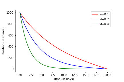
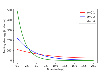
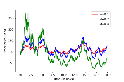
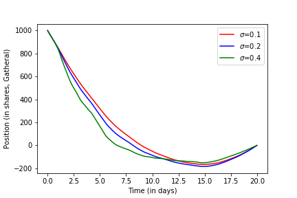
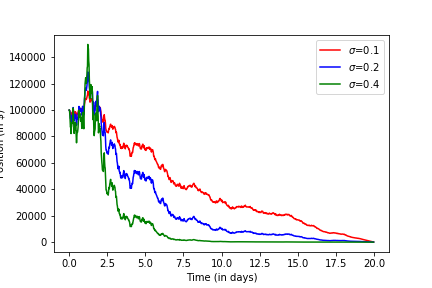
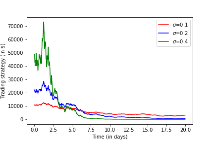
We simulate one Brownian motion trajectory, and plot the corresponding stock price process, as well as trading strategy (ut)t[0,T]subscriptsuperscriptsubscript𝑢𝑡𝑡0𝑇(u_{t}^{\star})_{t\in[0,T]} and trader’s cash position (θt)t[0,T]subscriptsuperscriptsubscript𝜃𝑡𝑡0𝑇(\theta_{t}^{\star})_{t\in[0,T]} and in shares (θt/St)t[0,T]subscriptsuperscriptsubscript𝜃𝑡subscript𝑆𝑡𝑡0𝑇(\theta_{t}^{\star}/S_{t})_{t\in[0,T]} for different values of σ𝜎\sigma. We take a stock with initial price S0=100$subscript𝑆0100currency-dollarS_{0}=100\$ following a GBM without drift (whose trajectories for different values of σ𝜎\sigma are in Figure 6), a portfolio of 103superscript10310^{3} shares to liquidate over T=20𝑇20T=20 days, with λ=κ=0.2𝜆𝜅0.2\lambda=\kappa=0.2. In Figure 2, we see an increase of the cash position at the beginning, which can be misleading but is only due to the initial increase of the stock price process. This is also represented in the trading strategy of Figure 2, where we see that the trader liquidates his position faster when the stock process has a higher volatility. Figures 4 and 4 show the position and the trading strategy in terms of shares. We also compare in Figure 6 our trading strategy in shares to the one in [7], which is defined as

qt:=(TtT)(q0κT40tSudu),assignsuperscriptsubscript𝑞𝑡𝑇𝑡𝑇subscript𝑞0𝜅𝑇4superscriptsubscript0𝑡subscript𝑆𝑢differential-d𝑢\displaystyle q_{t}^{\star}:=\big{(}\frac{T-t}{T}\big{)}\Big{(}q_{0}-\frac{\kappa T}{4}\int_{0}^{t}S_{u}\mathrm{d}u\Big{)}, (4.1)

where q0=θ0S0subscript𝑞0subscript𝜃0subscript𝑆0q_{0}=\frac{\theta_{0}}{S_{0}} is the initial number of shares hold by the trader, and dSt=σStdWtdsubscript𝑆𝑡𝜎subscript𝑆𝑡dsubscript𝑊𝑡\mathrm{d}S_{t}=\sigma S_{t}\mathrm{d}W_{t}. The trader still liquidates faster with a high volatility but his trading strategy, in this rather extreme regime, can go negative.
Refer to caption
Figure 1: Evolution of the cash position with respect to time.
Refer to caption
Figure 2: Trading strategy in cash with respect to time.
Refer to caption
Figure 3: Evolution of the share’s position with respect to time.
Refer to caption
Figure 4: Trading strategy in shares with respect to time.
Refer to caption
Figure 5: Evolution of the stock price with respect to time.
Refer to caption
Figure 6: Evolution of the share’s position with respect to time using (4.1).

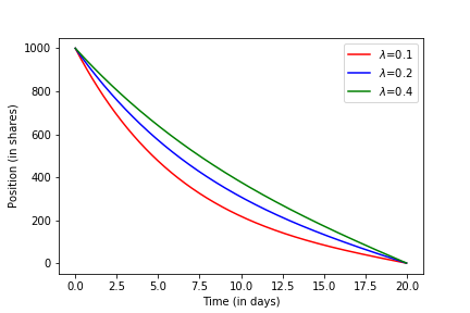
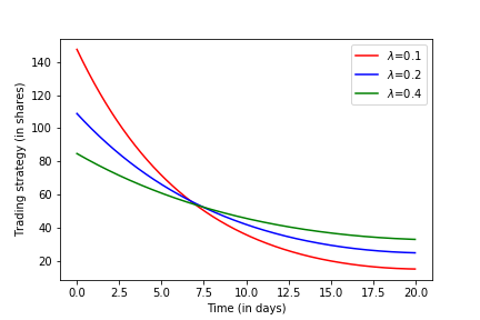
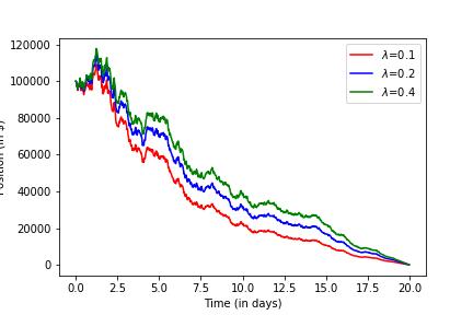
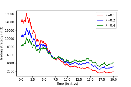
We now fix σ=0.1𝜎0.1\sigma=0.1 and κ=0.2𝜅0.2\kappa=0.2. The various cases of the impact of the transaction costs λ𝜆\lambda on the trader’s behavior are represented in Figures 8,8,10 and 10. Obviously, the price process is insensitive to a variation of λ𝜆\lambda. Moreover, the trading strategies in Figures 8 and 10 are decreasing functions of λ𝜆\lambda meaning that the trader liquidates his position using smaller sell orders when transactions costs are higher. This is also shown in the trader’s position in Figures 8 and 10.
Refer to caption
Figure 7: Evolution of the cash position with respect to time.
Refer to caption
Figure 8: Trading strategy in cash with respect to time.
Refer to caption
Figure 9: Evolution of the share’s position with respect to time.
Refer to caption
Figure 10: Trading strategy in shares with respect to time.

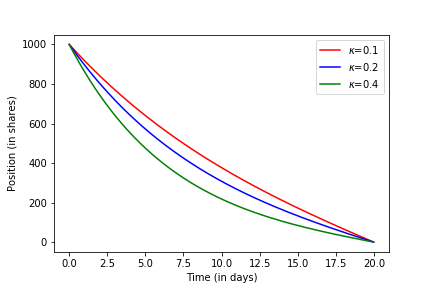
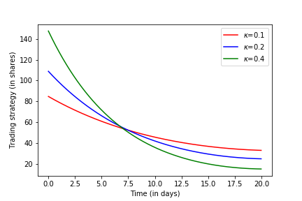
Finally, we set σ=0.1,λ=0.2formulae-sequence𝜎0.1𝜆0.2\sigma=0.1,\lambda=0.2 and study the influence of the risk aversion parameter κ𝜅\kappa. In Figures 12 and 14, we see that a highly risk averse trader will liquidate faster than a low risk averse trader. This is shown in terms of his position in Figures 12 and 14.
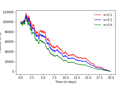
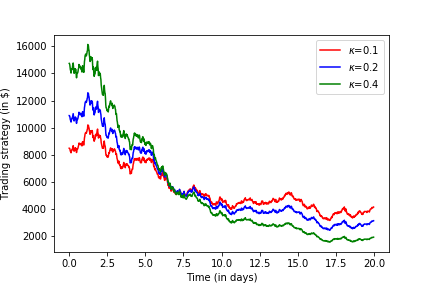
Refer to caption
Figure 11: Evolution of the cash position with respect to time.
Refer to caption
Figure 12: Trading strategy in cash with respect to time.
Refer to caption
Figure 13: Evolution of the share’s position with respect to time.
Refer to caption
Figure 14: Trading strategy in shares with respect to time.

We now show how to extend our framework to the case of a stochastic drift for the price process and the liquidation of a portfolio of N𝑁N assets.

5 Extensions of the model

5.1 Stochastic drift

We now consider the case of a stochastic drift, that is we solve

lima+supu𝒜𝔼[0Tαtθt(λ2ut2+κσ22(θtu)2)dta2(θTu)2],subscript𝑎subscriptsupremum𝑢𝒜𝔼delimited-[]superscriptsubscript0𝑇subscript𝛼𝑡subscript𝜃𝑡𝜆2superscriptsubscript𝑢𝑡2𝜅superscript𝜎22superscriptsuperscriptsubscript𝜃𝑡𝑢2d𝑡𝑎2superscriptsuperscriptsubscript𝜃𝑇𝑢2\displaystyle\lim_{a\rightarrow+\infty}\sup_{u\in\mathcal{A}}\mathbb{E}\Big{[}\int_{0}^{T}\alpha_{t}\theta_{t}-\Big{(}\frac{\lambda}{2}u_{t}^{2}+\frac{\kappa\sigma^{2}}{2}(\theta_{t}^{u})^{2}\Big{)}\mathrm{d}t-\frac{a}{2}(\theta_{T}^{u})^{2}\Big{]},

where (αt)t[0,T]subscriptsubscript𝛼𝑡𝑡0𝑇(\alpha_{t})_{t\in[0,T]} is a stochastic drift of the price process. We consider a slight modification of the problem where we neglect the part αtStsubscript𝛼𝑡subscript𝑆𝑡\alpha_{t}S_{t} of the price’s drift.555It can be shown that, if there exists η>0𝜂0\eta>0 such that supt|αt|<ηsubscriptsupremum𝑡subscript𝛼𝑡𝜂\sup_{t}|\alpha_{t}|<\eta, then the trading strategy derived in this section is arbitrary closed (as a function of η,T,σ𝜂𝑇𝜎\eta,T,\sigma) to the optimal strategy without simplification of the drift. Therefore, we simplify the dynamics of the price process, and assume

dθtu=utdt+σθtudWt.dsuperscriptsubscript𝜃𝑡𝑢subscript𝑢𝑡d𝑡𝜎superscriptsubscript𝜃𝑡𝑢dsubscript𝑊𝑡\displaystyle\mathrm{d}\theta_{t}^{u}=u_{t}\mathrm{d}t+\sigma\theta_{t}^{u}\mathrm{d}W_{t}. (5.1)

The first-order condition associated to this optimization problem writes as

κσ2λsT0t𝔼[MtMτ1uτ|s]dτdt+us+aλMT0TMτ1uτdτ=1λsT𝔼[αt|s]dt.𝜅superscript𝜎2𝜆superscriptsubscript𝑠𝑇superscriptsubscript0𝑡superscript𝔼delimited-[]conditionalsubscript𝑀𝑡superscriptsubscript𝑀𝜏1subscript𝑢𝜏subscript𝑠differential-d𝜏differential-d𝑡subscript𝑢𝑠𝑎𝜆subscript𝑀𝑇superscriptsubscript0𝑇superscriptsubscript𝑀𝜏1subscript𝑢𝜏differential-d𝜏1𝜆superscriptsubscript𝑠𝑇superscript𝔼delimited-[]conditionalsubscript𝛼𝑡subscript𝑠differential-d𝑡\displaystyle\frac{\kappa\sigma^{2}}{\lambda}\int_{s}^{T}\int_{0}^{t}\mathbb{E}^{\mathbb{Q}}[M_{t}M_{\tau}^{-1}u_{\tau}|\mathcal{F}_{s}]\mathrm{d}\tau\mathrm{d}t+u_{s}+\frac{a}{\lambda}M_{T}\int_{0}^{T}M_{\tau}^{-1}u_{\tau}\mathrm{d}\tau=\frac{1}{\lambda}\int_{s}^{T}\mathbb{E}^{\mathbb{Q}}[\alpha_{t}|\mathcal{F}_{s}]\mathrm{d}t.

Then, the analogous of Equation (3.2) can be rewritten

v(s)+κσ2λsTz(t)dt+aλz(T)=1λsT𝔼[αt|s0]dt.𝑣𝑠𝜅superscript𝜎2𝜆superscriptsubscript𝑠𝑇𝑧𝑡differential-d𝑡𝑎𝜆𝑧𝑇1𝜆superscriptsubscript𝑠𝑇superscript𝔼delimited-[]conditionalsubscript𝛼𝑡subscriptsubscript𝑠0differential-d𝑡\displaystyle v(s)+\frac{\kappa\sigma^{2}}{\lambda}\int_{s}^{T}z(t)\mathrm{d}t+\frac{a}{\lambda}z(T)=\frac{1}{\lambda}\int_{s}^{T}\mathbb{E}^{\mathbb{Q}}[\alpha_{t}|\mathcal{F}_{s_{0}}]\mathrm{d}t.

where the couple (v,z)𝑣𝑧(v,z) satisfies the following system of differential equations

{v(s)=κσ2λz(s)1λ𝔼[αs|s0]z(s)=σ2z(s)+v(s),casessuperscript𝑣𝑠𝜅superscript𝜎2𝜆𝑧𝑠1𝜆superscript𝔼delimited-[]conditionalsubscript𝛼𝑠subscriptsubscript𝑠0missing-subexpressionsuperscript𝑧𝑠superscript𝜎2𝑧𝑠𝑣𝑠missing-subexpression\displaystyle\left\{\begin{array}[]{ll}v^{\prime}(s)=\frac{\kappa\sigma^{2}}{\lambda}z(s)-\frac{1}{\lambda}\mathbb{E}^{\mathbb{Q}}[\alpha_{s}|\mathcal{F}_{s_{0}}]\\ z^{\prime}(s)=\sigma^{2}z(s)+v(s),\\ \end{array}\right.

with conditions

{v(T)=aλz(T)z(s0)=θs0.cases𝑣𝑇𝑎𝜆𝑧𝑇missing-subexpression𝑧subscript𝑠0subscript𝜃subscript𝑠0missing-subexpression\displaystyle\left\{\begin{array}[]{ll}v(T)=-\frac{a}{\lambda}z(T)\\ z(s_{0})=\theta_{s_{0}}.\\ \end{array}\right.

We finally obtain the following theorem:

Theorem 5.1.

The optimal control at any time t[0,T]𝑡0𝑇t\in[0,T] is given by

ut=θtuΓ(t)+ν(t),subscriptsuperscript𝑢𝑡superscriptsubscript𝜃𝑡superscript𝑢Γ𝑡𝜈𝑡\displaystyle u^{\star}_{t}=\theta_{t}^{u^{\star}}\Gamma(t)+\nu(t),

where the optimal trader’s position is defined as

θtu=Ht0tHs1ν(s)dssuperscriptsubscript𝜃𝑡superscript𝑢subscript𝐻𝑡superscriptsubscript0𝑡superscriptsubscript𝐻𝑠1𝜈𝑠differential-d𝑠\displaystyle\theta_{t}^{u^{\star}}=H_{t}\int_{0}^{t}H_{s}^{-1}\nu(s)\mathrm{d}s

with dHt=Γ(t)Htdt+σHtdWtdsubscript𝐻𝑡Γ𝑡subscript𝐻𝑡d𝑡𝜎subscript𝐻𝑡dsubscript𝑊𝑡\mathrm{d}H_{t}=\Gamma(t)H_{t}\mathrm{d}t+\sigma H_{t}\mathrm{d}W_{t}, and Γ(),ν()Γ𝜈\Gamma(\cdot),\nu(\cdot) are deterministic functions defined in (LABEL:Definition_Gamma_nu).

The term ν()𝜈\nu(\cdot) is a linear function of both αtsubscript𝛼𝑡\alpha_{t} and 𝔼[αT|t]superscript𝔼delimited-[]conditionalsubscript𝛼𝑇subscript𝑡\mathbb{E}^{\mathbb{Q}}[\alpha_{T}|\mathcal{F}_{t}], representing the influence of the drift on the optimal strategy. It is an increasing function of the drift αtsubscript𝛼𝑡\alpha_{t} meaning that we aim at liquidating faster our position when the stock price increases. Moreover, it is a decreasing function of 𝔼[αT|t]superscript𝔼delimited-[]conditionalsubscript𝛼𝑇subscript𝑡\mathbb{E}^{\mathbb{Q}}[\alpha_{T}|\mathcal{F}_{t}]: when the expected drift at the terminal time is high, the trader prefers to liquidate slower, waiting for a future stock price increase. As in the zero-drift case, we observe an aggressive in-the-money selling strategy.

5.2 Multi-dimensional case

This model extends directly to the problem of optimal execution of a portfolio of N𝑁N assets. We define the return of the i𝑖i-th asset as

dyti=σidWti,dsuperscriptsubscript𝑦𝑡𝑖subscript𝜎𝑖dsuperscriptsubscript𝑊𝑡𝑖\displaystyle\mathrm{d}y_{t}^{i}=\sigma_{i}\mathrm{d}W_{t}^{i},

where (W1,,WN)superscript𝑊1superscript𝑊𝑁(W^{1},\dots,W^{N}) are Brownian motions with non singular covariance matrix Σ=(σiσjρi,j)1i,jNΣsubscriptsubscript𝜎𝑖subscript𝜎𝑗superscript𝜌𝑖𝑗formulae-sequence1𝑖𝑗𝑁\Sigma=(\sigma_{i}\sigma_{j}\rho^{i,j})_{1\leq i,j\leq N}, σi>0subscript𝜎𝑖0\sigma_{i}>0 is the volatility of the i𝑖i-th asset and ρi,jsuperscript𝜌𝑖𝑗\rho^{i,j} is the correlation between the i𝑖i-th and the j𝑗j-th Brownian motion. The cash position of the trader with respect to the i𝑖i-th asset is defined by

dθtu,idsuperscriptsubscript𝜃𝑡𝑢𝑖\displaystyle\mathrm{d}\theta_{t}^{u,i} =utidt+θtu,idyti=utidt+σiθtu,idWti,absentsuperscriptsubscript𝑢𝑡𝑖d𝑡superscriptsubscript𝜃𝑡𝑢𝑖dsuperscriptsubscript𝑦𝑡𝑖superscriptsubscript𝑢𝑡𝑖d𝑡subscript𝜎𝑖superscriptsubscript𝜃𝑡𝑢𝑖dsuperscriptsubscript𝑊𝑡𝑖\displaystyle=u_{t}^{i}\mathrm{d}t+\theta_{t}^{u,i}\mathrm{d}y_{t}^{i}=u_{t}^{i}\mathrm{d}t+\sigma_{i}\theta_{t}^{u,i}\mathrm{d}W_{t}^{i}, (5.2)

where (uti)t[0,T]subscriptsuperscriptsubscript𝑢𝑡𝑖𝑡0𝑇(u_{t}^{i})_{t\in[0,T]} is the trading rate on the i𝑖i-th asset. Therefore the optimization problem (2.3) rewrites as

lima+supu𝒜𝔼[0Ti=1Nλ2(uti)2κ2(i=1Nσi2(θtu,i)2dt+i,j=1ijNρi,jσiσjθtu,iθtu,jdt)a2i=1N(θTu,i)2],subscript𝑎subscriptsupremum𝑢𝒜𝔼delimited-[]superscriptsubscript0𝑇superscriptsubscript𝑖1𝑁𝜆2superscriptsuperscriptsubscript𝑢𝑡𝑖2𝜅2superscriptsubscript𝑖1𝑁superscriptsubscript𝜎𝑖2superscriptsuperscriptsubscript𝜃𝑡𝑢𝑖2d𝑡superscriptsubscript𝑖𝑗1𝑖𝑗𝑁superscript𝜌𝑖𝑗subscript𝜎𝑖subscript𝜎𝑗superscriptsubscript𝜃𝑡𝑢𝑖superscriptsubscript𝜃𝑡𝑢𝑗d𝑡𝑎2superscriptsubscript𝑖1𝑁superscriptsuperscriptsubscript𝜃𝑇𝑢𝑖2\displaystyle\lim_{a\rightarrow+\infty}\sup_{u\in\mathcal{A}}\mathbb{E}\bigg{[}\int_{0}^{T}\sum_{i=1}^{N}-\frac{\lambda}{2}(u_{t}^{i})^{2}-\frac{\kappa}{2}\Big{(}\sum_{i=1}^{N}\sigma_{i}^{2}(\theta_{t}^{u,i})^{2}\mathrm{d}t+\sum_{\begin{subarray}{c}i,j=1\\ i\neq j\end{subarray}}^{N}\rho^{i,j}\sigma_{i}\sigma_{j}\theta_{t}^{u,i}\theta_{t}^{u,j}\mathrm{d}t\Big{)}-\frac{a}{2}\sum_{i=1}^{N}(\theta_{T}^{u,i})^{2}\bigg{]},

where

𝒜:={(uti)t[0,T],i{1,,N} measurable, s.t for all i{1,,N}0T|uti|dt<+,θTu,i=0}.assign𝒜conditional-setsubscriptsuperscriptsubscript𝑢𝑡𝑖formulae-sequence𝑡0𝑇𝑖1𝑁 measurable, s.t for all 𝑖1𝑁superscriptsubscript0𝑇formulae-sequenceconditionalsuperscriptsubscript𝑢𝑡𝑖d𝑡superscriptsubscript𝜃𝑇𝑢𝑖0\displaystyle\mathcal{A}:=\Big{\{}(u_{t}^{i})_{t\in[0,T],i\in\{1,\dots,N\}}\text{ measurable, s.t for all }i\in\{1,\dots,N\}\int_{0}^{T}|u_{t}^{i}|\mathrm{d}t<+\infty,\theta_{T}^{u,i}=0\Big{\}}.

We define (Kiuti)t[0,T],i{1,,N}subscriptsuperscript𝐾𝑖subscriptsuperscript𝑢𝑖𝑡formulae-sequence𝑡0𝑇𝑖1𝑁(K^{i}u^{i}_{t})_{t\in[0,T],i\in\{1,\dots,N\}} as the solution of the SDE (5.2):

(Kiui)t=Mti0t(Msi)1usids,subscriptsuperscript𝐾𝑖superscript𝑢𝑖𝑡superscriptsubscript𝑀𝑡𝑖superscriptsubscript0𝑡superscriptsuperscriptsubscript𝑀𝑠𝑖1subscriptsuperscript𝑢𝑖𝑠differential-d𝑠\displaystyle(K^{i}u^{i})_{t}=M_{t}^{i}\int_{0}^{t}(M_{s}^{i})^{-1}u^{i}_{s}\mathrm{d}s,

where did|T=MTi:=exp(σiWTi(σi)2T2)evaluated-atdsuperscript𝑖dsubscript𝑇superscriptsubscript𝑀𝑇𝑖assignsubscript𝜎𝑖superscriptsubscript𝑊𝑇𝑖superscriptsubscript𝜎𝑖2𝑇2\frac{\mathrm{d}\mathbb{Q}^{i}}{\mathrm{d}\mathbb{P}}\Big{|}_{\mathcal{F}_{T}}=M_{T}^{i}:=\exp\big{(}\sigma_{i}W_{T}^{i}-\frac{(\sigma_{i})^{2}T}{2}\big{)}. The adjoint operator is defined as

(Kiui)s=sT𝔼i[uti|s]dt.subscriptsuperscript𝐾absent𝑖superscript𝑢𝑖𝑠superscriptsubscript𝑠𝑇superscript𝔼superscript𝑖delimited-[]conditionalsubscriptsuperscript𝑢𝑖𝑡subscript𝑠differential-d𝑡\displaystyle(K^{\star i}u^{i})_{s}=\int_{s}^{T}\mathbb{E}^{\mathbb{Q}^{i}}[u^{i}_{t}|\mathcal{F}_{s}]\mathrm{d}t.

For a fixed a>0𝑎0a>0, the optimization problem rewrites

supu𝒜λ2u2κ2Ku,ΣKua2i=1N(Kiui)T2.subscriptsupremum𝑢𝒜𝜆2superscriptnorm𝑢2𝜅2𝐾𝑢Σ𝐾𝑢𝑎2superscriptsubscript𝑖1𝑁subscriptsuperscriptsuperscript𝐾𝑖superscript𝑢𝑖2𝑇\displaystyle\sup_{u\in\mathcal{A}}-\frac{\lambda}{2}\|u\|^{2}-\frac{\kappa}{2}\langle Ku,\Sigma Ku\rangle-\frac{a}{2}\sum_{i=1}^{N}(K^{i}u^{i})^{2}_{T}.

The first order condition gives the following system

ui+κ2λ(2σi2KiKiui+jiNρi,jσiσjKiKjuj)+aλ(Kiui)T=0,i=1,,N,formulae-sequencesuperscript𝑢𝑖𝜅2𝜆2superscriptsubscript𝜎𝑖2superscript𝐾absent𝑖superscript𝐾𝑖superscript𝑢𝑖superscriptsubscript𝑗𝑖𝑁superscript𝜌𝑖𝑗subscript𝜎𝑖subscript𝜎𝑗superscript𝐾absent𝑖superscript𝐾𝑗superscript𝑢𝑗𝑎𝜆subscriptsuperscript𝐾𝑖superscript𝑢𝑖𝑇0𝑖1𝑁\displaystyle u^{i}+\frac{\kappa}{2\lambda}\big{(}2\sigma_{i}^{2}K^{\star i}K^{i}u^{i}+\sum_{j\neq i}^{N}\rho^{i,j}\sigma_{i}\sigma_{j}K^{\star i}K^{j}u^{j}\big{)}+\frac{a}{\lambda}(K^{i}u^{i})_{T}=0,\quad i=1,\dots,N, (5.3)

or equivalently for all i=1,,N𝑖1𝑁i=1,\dots,N,

usi+κ2λ(2σi2sT0t(𝔼i[Mti(Mτi)1uτi|s]dτdt+jiNρi,jσiσj𝔼i[Mtj(Mτj)1uτj|s]dτdt))+aλ(Kiui)T=0.superscriptsubscript𝑢𝑠𝑖𝜅2𝜆2superscriptsubscript𝜎𝑖2superscriptsubscript𝑠𝑇superscriptsubscript0𝑡superscript𝔼superscript𝑖delimited-[]conditionalsuperscriptsubscript𝑀𝑡𝑖superscriptsuperscriptsubscript𝑀𝜏𝑖1superscriptsubscript𝑢𝜏𝑖subscript𝑠d𝜏d𝑡superscriptsubscript𝑗𝑖𝑁superscript𝜌𝑖𝑗subscript𝜎𝑖subscript𝜎𝑗superscript𝔼superscript𝑖delimited-[]conditionalsuperscriptsubscript𝑀𝑡𝑗superscriptsuperscriptsubscript𝑀𝜏𝑗1superscriptsubscript𝑢𝜏𝑗subscript𝑠d𝜏d𝑡𝑎𝜆subscriptsuperscript𝐾𝑖superscript𝑢𝑖𝑇0\displaystyle u_{s}^{i}+\frac{\kappa}{2\lambda}\Big{(}2\sigma_{i}^{2}\int_{s}^{T}\int_{0}^{t}\big{(}\mathbb{E}^{\mathbb{Q}^{i}}[M_{t}^{i}(M_{\tau}^{i})^{-1}u_{\tau}^{i}|\mathcal{F}_{s}]\mathrm{d}\tau\mathrm{d}t+\sum_{j\neq i}^{N}\rho^{i,j}\sigma_{i}\sigma_{j}\mathbb{E}^{\mathbb{Q}^{i}}[M_{t}^{j}(M_{\tau}^{j})^{-1}u_{\tau}^{j}|\mathcal{F}_{s}]\mathrm{d}\tau\mathrm{d}t\big{)}\Big{)}+\frac{a}{\lambda}(K^{i}u^{i})_{T}=0.

For any ss0𝑠subscript𝑠0s\geq s_{0}, apply 𝔼i[|s0]\mathbb{E}^{\mathbb{Q}^{i}}\big{[}\cdot|\mathcal{F}_{s_{0}}\big{]} on both sides of the equations. Simple but tedious computations lead to

𝔼i[usi|s0]+κσi2λ(sTeσi2(ts0)(Kiui)s0dt+sTs0teσi2(tτ)𝔼i[uτi|s0]dτdt)superscript𝔼superscript𝑖delimited-[]conditionalsubscriptsuperscript𝑢𝑖𝑠subscriptsubscript𝑠0𝜅superscriptsubscript𝜎𝑖2𝜆superscriptsubscript𝑠𝑇superscript𝑒superscriptsubscript𝜎𝑖2𝑡subscript𝑠0subscriptsuperscript𝐾𝑖superscript𝑢𝑖subscript𝑠0differential-d𝑡superscriptsubscript𝑠𝑇superscriptsubscriptsubscript𝑠0𝑡superscript𝑒superscriptsubscript𝜎𝑖2𝑡𝜏superscript𝔼superscript𝑖delimited-[]conditionalsuperscriptsubscript𝑢𝜏𝑖subscriptsubscript𝑠0differential-d𝜏differential-d𝑡\displaystyle\mathbb{E}^{\mathbb{Q}^{i}}\big{[}u^{i}_{s}|\mathcal{F}_{s_{0}}\big{]}+\frac{\kappa\sigma_{i}^{2}}{\lambda}\Big{(}\int_{s}^{T}e^{\sigma_{i}^{2}(t-s_{0})}(K^{i}u^{i})_{s_{0}}\mathrm{d}t+\int_{s}^{T}\int_{s_{0}}^{t}e^{\sigma_{i}^{2}(t-\tau)}\mathbb{E}^{\mathbb{Q}^{i}}\big{[}u_{\tau}^{i}|\mathcal{F}_{s_{0}}\big{]}\mathrm{d}\tau\mathrm{d}t\Big{)}
+κλjiNρi,jσiσj(sTeσiσjρi,j(ts0)(Kjuj)s0+sTs0teσiσjρi,j(tτ)𝔼j[uτj|s0]dτdt)𝜅𝜆superscriptsubscript𝑗𝑖𝑁superscript𝜌𝑖𝑗subscript𝜎𝑖subscript𝜎𝑗superscriptsubscript𝑠𝑇superscript𝑒subscript𝜎𝑖subscript𝜎𝑗superscript𝜌𝑖𝑗𝑡subscript𝑠0subscriptsuperscript𝐾𝑗superscript𝑢𝑗subscript𝑠0superscriptsubscript𝑠𝑇superscriptsubscriptsubscript𝑠0𝑡superscript𝑒subscript𝜎𝑖subscript𝜎𝑗superscript𝜌𝑖𝑗𝑡𝜏superscript𝔼superscript𝑗delimited-[]conditionalsuperscriptsubscript𝑢𝜏𝑗subscriptsubscript𝑠0differential-d𝜏differential-d𝑡\displaystyle+\frac{\kappa}{\lambda}\sum_{j\neq i}^{N}\rho^{i,j}\sigma_{i}\sigma_{j}\Big{(}\int_{s}^{T}e^{\sigma_{i}\sigma_{j}\rho^{i,j}(t-s_{0})}(K^{j}u^{j})_{s_{0}}+\int_{s}^{T}\int_{s_{0}}^{t}e^{\sigma_{i}\sigma_{j}\rho^{i,j}(t-\tau)}\mathbb{E}^{\mathbb{Q}^{j}}\big{[}u_{\tau}^{j}|\mathcal{F}_{s_{0}}\big{]}\mathrm{d}\tau\mathrm{d}t\Big{)}
+aλ(eσi2(Ts0)(Kiui)s0+s0Teσi2(Tτ)𝔼i[uτi|s0]dτ)=0.𝑎𝜆superscript𝑒superscriptsubscript𝜎𝑖2𝑇subscript𝑠0subscriptsuperscript𝐾𝑖superscript𝑢𝑖subscript𝑠0superscriptsubscriptsubscript𝑠0𝑇superscript𝑒superscriptsubscript𝜎𝑖2𝑇𝜏superscript𝔼superscript𝑖delimited-[]conditionalsuperscriptsubscript𝑢𝜏𝑖subscriptsubscript𝑠0differential-d𝜏0\displaystyle+\frac{a}{\lambda}\Big{(}e^{\sigma_{i}^{2}(T-s_{0})}(K^{i}u^{i})_{s_{0}}+\int_{s_{0}}^{T}e^{\sigma_{i}^{2}(T-\tau)}\mathbb{E}^{\mathbb{Q}^{i}}\big{[}u_{\tau}^{i}|\mathcal{F}_{s_{0}}\big{]}\mathrm{d}\tau\Big{)}=0.

By denoting for all i=1,,N𝑖1𝑁i=1,\dots,N, vi(s)=𝔼i[usi|s0]superscript𝑣𝑖𝑠superscript𝔼superscript𝑖delimited-[]conditionalsuperscriptsubscript𝑢𝑠𝑖subscriptsubscript𝑠0v^{i}(s)=\mathbb{E}^{\mathbb{Q}^{i}}\big{[}u_{s}^{i}|\mathcal{F}_{s_{0}}\big{]}, and θs0i=(Kiui)s0superscriptsubscript𝜃subscript𝑠0𝑖subscriptsuperscript𝐾𝑖superscript𝑢𝑖subscript𝑠0\theta_{s_{0}}^{i}=(K^{i}u^{i})_{s_{0}} the system becomes

vi(s)+κσi2λ(sTeσi2(ts0)θs0idt+sTs0teσi2(tτ)vi(τ)dτdt)superscript𝑣𝑖𝑠𝜅superscriptsubscript𝜎𝑖2𝜆superscriptsubscript𝑠𝑇superscript𝑒superscriptsubscript𝜎𝑖2𝑡subscript𝑠0subscriptsuperscript𝜃𝑖subscript𝑠0differential-d𝑡superscriptsubscript𝑠𝑇superscriptsubscriptsubscript𝑠0𝑡superscript𝑒superscriptsubscript𝜎𝑖2𝑡𝜏superscript𝑣𝑖𝜏differential-d𝜏differential-d𝑡\displaystyle v^{i}(s)+\frac{\kappa\sigma_{i}^{2}}{\lambda}\Big{(}\int_{s}^{T}e^{\sigma_{i}^{2}(t-s_{0})}\theta^{i}_{s_{0}}\mathrm{d}t+\int_{s}^{T}\int_{s_{0}}^{t}e^{\sigma_{i}^{2}(t-\tau)}v^{i}(\tau)\mathrm{d}\tau\mathrm{d}t\Big{)}
+κλjiNρi,jσiσj(sTeσiσjρi,j(ts0)θs0j+sTs0teσiσjρi,j(tτ)vj(τ)dτdt)𝜅𝜆superscriptsubscript𝑗𝑖𝑁superscript𝜌𝑖𝑗subscript𝜎𝑖subscript𝜎𝑗superscriptsubscript𝑠𝑇superscript𝑒subscript𝜎𝑖subscript𝜎𝑗superscript𝜌𝑖𝑗𝑡subscript𝑠0subscriptsuperscript𝜃𝑗subscript𝑠0superscriptsubscript𝑠𝑇superscriptsubscriptsubscript𝑠0𝑡superscript𝑒subscript𝜎𝑖subscript𝜎𝑗superscript𝜌𝑖𝑗𝑡𝜏superscript𝑣𝑗𝜏differential-d𝜏differential-d𝑡\displaystyle+\frac{\kappa}{\lambda}\sum_{j\neq i}^{N}\rho^{i,j}\sigma_{i}\sigma_{j}\Big{(}\int_{s}^{T}e^{\sigma_{i}\sigma_{j}\rho^{i,j}(t-s_{0})}\theta^{j}_{s_{0}}+\int_{s}^{T}\int_{s_{0}}^{t}e^{\sigma_{i}\sigma_{j}\rho^{i,j}(t-\tau)}v^{j}(\tau)\mathrm{d}\tau\mathrm{d}t\Big{)}
+aλ(eσi2(Ts0)θs0i+s0Teσi2(Tτ)vi(τ)dτ)=0.𝑎𝜆superscript𝑒superscriptsubscript𝜎𝑖2𝑇subscript𝑠0subscriptsuperscript𝜃𝑖subscript𝑠0superscriptsubscriptsubscript𝑠0𝑇superscript𝑒superscriptsubscript𝜎𝑖2𝑇𝜏superscript𝑣𝑖𝜏differential-d𝜏0\displaystyle+\frac{a}{\lambda}\Big{(}e^{\sigma_{i}^{2}(T-s_{0})}\theta^{i}_{s_{0}}+\int_{s_{0}}^{T}e^{\sigma_{i}^{2}(T-\tau)}v^{i}(\tau)\mathrm{d}\tau\Big{)}=0.

We define

zi(t):=eσi2(ts0)θs0i+s0teσi2(tτ)vi(τ)dτ,assignsuperscript𝑧𝑖𝑡superscript𝑒superscriptsubscript𝜎𝑖2𝑡subscript𝑠0subscriptsuperscript𝜃𝑖subscript𝑠0superscriptsubscriptsubscript𝑠0𝑡superscript𝑒superscriptsubscript𝜎𝑖2𝑡𝜏superscript𝑣𝑖𝜏differential-d𝜏\displaystyle z^{i}(t):=e^{\sigma_{i}^{2}(t-s_{0})}\theta^{i}_{s_{0}}+\int_{s_{0}}^{t}e^{\sigma_{i}^{2}(t-\tau)}v^{i}(\tau)\mathrm{d}\tau,
zi,j(t):=eσiσjρi,j(ts0)θs0j+s0teσiσjρi,j(tτ)vj(τ)dτ,assignsuperscript𝑧𝑖𝑗𝑡superscript𝑒subscript𝜎𝑖subscript𝜎𝑗superscript𝜌𝑖𝑗𝑡subscript𝑠0subscriptsuperscript𝜃𝑗subscript𝑠0superscriptsubscriptsubscript𝑠0𝑡superscript𝑒subscript𝜎𝑖subscript𝜎𝑗superscript𝜌𝑖𝑗𝑡𝜏superscript𝑣𝑗𝜏differential-d𝜏\displaystyle z^{i,j}(t):=e^{\sigma_{i}\sigma_{j}\rho^{i,j}(t-s_{0})}\theta^{j}_{s_{0}}+\int_{s_{0}}^{t}e^{\sigma_{i}\sigma_{j}\rho^{i,j}(t-\tau)}v^{j}(\tau)\mathrm{d}\tau,

and obtain for all i=1,,N𝑖1𝑁i=1,\dots,N:

vi(s)+κσi2λ(sTzi(t)dt)+κλjiNρi,jσiσjsTzi,j(t)dt+aλzi(T)=0.superscript𝑣𝑖𝑠𝜅superscriptsubscript𝜎𝑖2𝜆superscriptsubscript𝑠𝑇superscript𝑧𝑖𝑡differential-d𝑡𝜅𝜆superscriptsubscript𝑗𝑖𝑁superscript𝜌𝑖𝑗subscript𝜎𝑖subscript𝜎𝑗superscriptsubscript𝑠𝑇superscript𝑧𝑖𝑗𝑡differential-d𝑡𝑎𝜆superscript𝑧𝑖𝑇0\displaystyle v^{i}(s)+\frac{\kappa\sigma_{i}^{2}}{\lambda}\Big{(}\int_{s}^{T}z^{i}(t)\mathrm{d}t\Big{)}+\frac{\kappa}{\lambda}\sum_{j\neq i}^{N}\rho^{i,j}\sigma_{i}\sigma_{j}\int_{s}^{T}z^{i,j}(t)\mathrm{d}t+\frac{a}{\lambda}z^{i}(T)=0.

Therefore first-order condition (5.3) is equivalent to the system of differential equations

{vi(s)κσi2λzi(s)κλjiNρi,jσiσjzi,j(s)=0zi(s)=σi2zi(s)+vi(s)zi,j(s)=σiσjρi,jzi,j(s)+vj(s),casessuperscript𝑣superscript𝑖𝑠𝜅superscriptsubscript𝜎𝑖2𝜆superscript𝑧𝑖𝑠𝜅𝜆superscriptsubscript𝑗𝑖𝑁superscript𝜌𝑖𝑗subscript𝜎𝑖subscript𝜎𝑗superscript𝑧𝑖𝑗𝑠0missing-subexpressionsuperscript𝑧superscript𝑖𝑠superscriptsubscript𝜎𝑖2superscript𝑧𝑖𝑠superscript𝑣𝑖𝑠missing-subexpressionsuperscript𝑧superscript𝑖𝑗𝑠subscript𝜎𝑖subscript𝜎𝑗superscript𝜌𝑖𝑗superscript𝑧𝑖𝑗𝑠superscript𝑣𝑗𝑠missing-subexpression\displaystyle\left\{\begin{array}[]{ll}v^{{}^{\prime}i}(s)-\frac{\kappa\sigma_{i}^{2}}{\lambda}z^{i}(s)-\frac{\kappa}{\lambda}\sum_{j\neq i}^{N}\rho^{i,j}\sigma_{i}\sigma_{j}z^{i,j}(s)=0\\ z^{{}^{\prime}i}(s)=\sigma_{i}^{2}z^{i}(s)+v^{i}(s)\\ z^{{}^{\prime}i,j}(s)=\sigma_{i}\sigma_{j}\rho^{i,j}z^{i,j}(s)+v^{j}(s),\\ \end{array}\right.

with initial conditions

{vi(T)=aλzi(T)zi(s0)=θs0izi,j(s0)=θs0j.casessuperscript𝑣𝑖𝑇𝑎𝜆superscript𝑧𝑖𝑇missing-subexpressionsuperscript𝑧𝑖subscript𝑠0superscriptsubscript𝜃subscript𝑠0𝑖missing-subexpressionsuperscript𝑧𝑖𝑗subscript𝑠0superscriptsubscript𝜃subscript𝑠0𝑗missing-subexpression\displaystyle\left\{\begin{array}[]{ll}v^{i}(T)=-\frac{a}{\lambda}z^{i}(T)\\ z^{i}(s_{0})=\theta_{s_{0}}^{i}\\ z^{i,j}(s_{0})=\theta_{s_{0}}^{j}.\\ \end{array}\right.

We obtain a system of linear differential equations with constant coefficients. Thus, by noting that for all i=1,,N𝑖1𝑁i=1,\dots,N and s0[0,T]subscript𝑠00𝑇s_{0}\in[0,T], vi(s0)=us0isuperscript𝑣𝑖subscript𝑠0superscriptsubscript𝑢subscript𝑠0𝑖v^{i}(s_{0})=u_{s_{0}}^{i}, we obtain the controls utisuperscriptsubscript𝑢𝑡𝑖u_{t}^{i} for all t[0,T]𝑡0𝑇t\in[0,T] and i=1,,N𝑖1𝑁i=1,\dots,N by solving this system of ODEs.

6 Conclusion

In this article, we present a way to solve the traditional Almgren-Chriss liquidation problem when the underlying asset is driven by a GBM. By working in terms of cash and using functional analysis tools, we can provide the optimal control of the problem explicitly. We provide an extension to the case of a GBM with stochastic drift and the liquidation of a portfolio of correlated assets. In particular, our method does not suffer from the curse of dimensionality.

A Appendix

A.1 Proof of Lemma 3.1

An application of Ito’s formula gives

d(Ku)t=utdt+σ(Ku)tdWt,dsubscript𝐾𝑢𝑡subscript𝑢𝑡d𝑡𝜎subscript𝐾𝑢𝑡dsubscript𝑊𝑡\displaystyle\mathrm{d}(Ku)_{t}=u_{t}\mathrm{d}t+\sigma(Ku)_{t}\mathrm{d}W_{t},

hence solving (2.2). The adjoint of K𝐾K is the operator Ksuperscript𝐾K^{\star} such that for all (u,v)𝒜𝑢𝑣𝒜(u,v)\in\mathcal{A},

Ku,v=u,Kv.𝐾𝑢𝑣𝑢superscript𝐾𝑣\displaystyle\langle Ku,v\rangle=\langle u,K^{\star}v\rangle.

Using Bayes formula, we have

Ku,v𝐾𝑢𝑣\displaystyle\langle Ku,v\rangle =𝔼[0T(Ku)tvtdt]absent𝔼delimited-[]superscriptsubscript0𝑇subscript𝐾𝑢𝑡subscript𝑣𝑡differential-d𝑡\displaystyle=\mathbb{E}\Big{[}\int_{0}^{T}(Ku)_{t}v_{t}\mathrm{d}t\Big{]}
=𝔼[0T0tMtMs1usvtdsdt]absent𝔼delimited-[]superscriptsubscript0𝑇superscriptsubscript0𝑡subscript𝑀𝑡superscriptsubscript𝑀𝑠1subscript𝑢𝑠subscript𝑣𝑡differential-d𝑠differential-d𝑡\displaystyle=\mathbb{E}\Big{[}\int_{0}^{T}\int_{0}^{t}M_{t}M_{s}^{-1}u_{s}v_{t}\mathrm{d}s\mathrm{d}t\Big{]}
=𝔼[0TsTMtMs1usvtdtds]absent𝔼delimited-[]superscriptsubscript0𝑇superscriptsubscript𝑠𝑇subscript𝑀𝑡superscriptsubscript𝑀𝑠1subscript𝑢𝑠subscript𝑣𝑡differential-d𝑡differential-d𝑠\displaystyle=\mathbb{E}\Big{[}\int_{0}^{T}\int_{s}^{T}M_{t}M_{s}^{-1}u_{s}v_{t}\mathrm{d}t\mathrm{d}s\Big{]}
=𝔼[0Tus(Kv)sds]absent𝔼delimited-[]superscriptsubscript0𝑇subscript𝑢𝑠subscriptsuperscript𝐾𝑣𝑠differential-d𝑠\displaystyle=\mathbb{E}\Big{[}\int_{0}^{T}u_{s}(K^{\star}v)_{s}\mathrm{d}s\Big{]}
=u,Kv,absent𝑢superscript𝐾𝑣\displaystyle=\langle u,K^{\star}v\rangle,

where (Kv)s=sTMtMs1vtdt=sT𝔼[vt|s]dtsubscriptsuperscript𝐾𝑣𝑠superscriptsubscript𝑠𝑇subscript𝑀𝑡subscriptsuperscript𝑀1𝑠subscript𝑣𝑡differential-d𝑡superscriptsubscript𝑠𝑇superscript𝔼delimited-[]conditionalsubscript𝑣𝑡subscript𝑠differential-d𝑡(K^{\star}v)_{s}=\int_{s}^{T}M_{t}M^{-1}_{s}v_{t}\mathrm{d}t=\int_{s}^{T}\mathbb{E}^{\mathbb{Q}}[v_{t}|\mathcal{F}_{s}]\mathrm{d}t.

A.2 Gateaux differentiability in (3.1)

We define the map Ξ:2:Ξsuperscript2\Xi:\mathbb{H}^{2}\rightarrow\mathbb{R} by

Ξ(u)=λ2u2κσ22Ku2a2(Ku)2.Ξ𝑢𝜆2superscriptnorm𝑢2𝜅superscript𝜎22superscriptnorm𝐾𝑢2𝑎2superscript𝐾𝑢2\displaystyle\Xi(u)=-\frac{\lambda}{2}\|u\|^{2}-\frac{\kappa\sigma^{2}}{2}\|Ku\|^{2}-\frac{a}{2}(Ku)^{2}.

As K𝐾K is a linear operator of u2𝑢superscript2u\in\mathbb{H}^{2}, and λ,κ>0𝜆𝜅0\lambda,\kappa>0, we deduce that ΞΞ\Xi is continuous, strictly concave and Gateaux differentiable; with Gateaux derivative given, for any h2superscript2h\in\mathbb{H}^{2}, by

Ξ(u)[h]=λu,hκσ2Ku,Kha(Kh).Ξ𝑢delimited-[]𝜆𝑢𝜅superscript𝜎2𝐾𝑢𝐾𝑎𝐾\displaystyle\Xi(u)[h]=-\lambda\langle u,h\rangle-\kappa\sigma^{2}\langle Ku,Kh\rangle-a(Kh).

By setting Ξ(u)[h]=0Ξ𝑢delimited-[]0\Xi(u)[h]=0, and using the definition of an adjoint operator, we obtain Equation (3.2).

A.3 Proof of Lemma 3.2

By the fact that

𝔼[sT0t𝔼[MtMτ1uτ|s]dτdt|s0]superscript𝔼delimited-[]conditionalsuperscriptsubscript𝑠𝑇superscriptsubscript0𝑡superscript𝔼delimited-[]conditionalsubscript𝑀𝑡superscriptsubscript𝑀𝜏1subscript𝑢𝜏subscript𝑠differential-d𝜏differential-d𝑡subscriptsubscript𝑠0\displaystyle\mathbb{E}^{\mathbb{Q}}\Big{[}\int_{s}^{T}\int_{0}^{t}\mathbb{E}^{\mathbb{Q}}[M_{t}M_{\tau}^{-1}u_{\tau}|\mathcal{F}_{s}]\mathrm{d}\tau\mathrm{d}t\big{|}\mathcal{F}_{s_{0}}\Big{]} =sT0t𝔼[MtMτ1uτ|s0]dτdtabsentsuperscriptsubscript𝑠𝑇superscriptsubscript0𝑡superscript𝔼delimited-[]conditionalsubscript𝑀𝑡superscriptsubscript𝑀𝜏1subscript𝑢𝜏subscriptsubscript𝑠0differential-d𝜏differential-d𝑡\displaystyle=\int_{s}^{T}\int_{0}^{t}\mathbb{E}^{\mathbb{Q}}[M_{t}M_{\tau}^{-1}u_{\tau}|\mathcal{F}_{s_{0}}]\mathrm{d}\tau\mathrm{d}t
=sT(0s0Mτ1uτ𝔼[Mt|s0]dτ+s0t𝔼[MtMτ1uτ|s0]dτ)dtabsentsuperscriptsubscript𝑠𝑇superscriptsubscript0subscript𝑠0superscriptsubscript𝑀𝜏1subscript𝑢𝜏superscript𝔼delimited-[]conditionalsubscript𝑀𝑡subscriptsubscript𝑠0differential-d𝜏superscriptsubscriptsubscript𝑠0𝑡superscript𝔼delimited-[]conditionalsubscript𝑀𝑡superscriptsubscript𝑀𝜏1subscript𝑢𝜏subscriptsubscript𝑠0differential-d𝜏differential-d𝑡\displaystyle=\int_{s}^{T}\Big{(}\int_{0}^{s_{0}}M_{\tau}^{-1}u_{\tau}\mathbb{E}^{\mathbb{Q}}[M_{t}|\mathcal{F}_{s_{0}}]\mathrm{d}\tau+\int_{s_{0}}^{t}\mathbb{E}^{\mathbb{Q}}[M_{t}M_{\tau}^{-1}u_{\tau}|\mathcal{F}_{s_{0}}]\mathrm{d}\tau\Big{)}\mathrm{d}t
=sT(eσ2(ts0)(Ku)s0dt+s0t𝔼[𝔼[MtMτ1uτ|s0]|τ]dτ)dtabsentsuperscriptsubscript𝑠𝑇superscript𝑒superscript𝜎2𝑡subscript𝑠0subscript𝐾𝑢subscript𝑠0d𝑡superscriptsubscriptsubscript𝑠0𝑡superscript𝔼delimited-[]conditionalsuperscript𝔼delimited-[]conditionalsubscript𝑀𝑡superscriptsubscript𝑀𝜏1subscript𝑢𝜏subscriptsubscript𝑠0subscript𝜏differential-d𝜏differential-d𝑡\displaystyle=\int_{s}^{T}\Big{(}e^{\sigma^{2}(t-s_{0})}(Ku)_{s_{0}}\mathrm{d}t+\int_{s_{0}}^{t}\mathbb{E}^{\mathbb{Q}}\big{[}\mathbb{E}^{\mathbb{Q}}[M_{t}M_{\tau}^{-1}u_{\tau}|\mathcal{F}_{s_{0}}]|\mathcal{F}_{\tau}\big{]}\mathrm{d}\tau\Big{)}\mathrm{d}t
=sT(eσ2(ts0)(Ku)s0dt+s0teσ2(tτ)𝔼[uτ|s0]dτ)dt.absentsuperscriptsubscript𝑠𝑇superscript𝑒superscript𝜎2𝑡subscript𝑠0subscript𝐾𝑢subscript𝑠0d𝑡superscriptsubscriptsubscript𝑠0𝑡superscript𝑒superscript𝜎2𝑡𝜏superscript𝔼delimited-[]conditionalsubscript𝑢𝜏subscriptsubscript𝑠0differential-d𝜏differential-d𝑡\displaystyle=\int_{s}^{T}\Big{(}e^{\sigma^{2}(t-s_{0})}(Ku)_{s_{0}}\mathrm{d}t+\int_{s_{0}}^{t}e^{\sigma^{2}(t-\tau)}\mathbb{E}^{\mathbb{Q}}[u_{\tau}|\mathcal{F}_{s_{0}}]\mathrm{d}\tau\Big{)}\mathrm{d}t.

Condition (3.3) can be rewritten

κσ2λsTeσ2(ts0)(Ku)s0dt+κσ2λsTs0teσ2(tτ)𝔼[uτ|s0]dτdt+aλeσ2(Ts0)θs0𝜅superscript𝜎2𝜆superscriptsubscript𝑠𝑇superscript𝑒superscript𝜎2𝑡subscript𝑠0subscript𝐾𝑢subscript𝑠0differential-d𝑡𝜅superscript𝜎2𝜆superscriptsubscript𝑠𝑇superscriptsubscriptsubscript𝑠0𝑡superscript𝑒superscript𝜎2𝑡𝜏superscript𝔼delimited-[]conditionalsubscript𝑢𝜏subscriptsubscript𝑠0differential-d𝜏differential-d𝑡𝑎𝜆superscript𝑒superscript𝜎2𝑇subscript𝑠0subscript𝜃subscript𝑠0\displaystyle\frac{\kappa\sigma^{2}}{\lambda}\int_{s}^{T}e^{\sigma^{2}(t-s_{0})}(Ku)_{s_{0}}\mathrm{d}t+\frac{\kappa\sigma^{2}}{\lambda}\int_{s}^{T}\int_{s_{0}}^{t}e^{\sigma^{2}(t-\tau)}\mathbb{E}^{\mathbb{Q}}[u_{\tau}|\mathcal{F}_{s_{0}}]\mathrm{d}\tau\mathrm{d}t+\frac{a}{\lambda}e^{\sigma^{2}(T-s_{0})}\theta_{s_{0}}
+aλs0Teσ2(Tτ)𝔼[uτ|s0]+𝔼[us|s0]=0,𝑎𝜆superscriptsubscriptsubscript𝑠0𝑇superscript𝑒superscript𝜎2𝑇𝜏superscript𝔼delimited-[]conditionalsubscript𝑢𝜏subscriptsubscript𝑠0superscript𝔼delimited-[]conditionalsubscript𝑢𝑠subscriptsubscript𝑠00\displaystyle+\frac{a}{\lambda}\int_{s_{0}}^{T}e^{\sigma^{2}(T-\tau)}\mathbb{E}^{\mathbb{Q}}[u_{\tau}|\mathcal{F}_{s_{0}}]+\mathbb{E}^{\mathbb{Q}}[u_{s}|\mathcal{F}_{s_{0}}]=0,

which proves the first statement of the theorem. We obtain the second point by a straightforward derivation of the functions z𝑧z and v𝑣v.

A.4 Proof of Theorem 5.1

The solution of the ODE for z𝑧z is given by

z(s)=θs0eσ2(ss0)+s0seσ2(su)v(u)du,𝑧𝑠subscript𝜃subscript𝑠0superscript𝑒superscript𝜎2𝑠subscript𝑠0superscriptsubscriptsubscript𝑠0𝑠superscript𝑒superscript𝜎2𝑠𝑢𝑣𝑢differential-d𝑢\displaystyle z(s)=\theta_{s_{0}}e^{\sigma^{2}(s-s_{0})}+\int_{s_{0}}^{s}e^{\sigma^{2}(s-u)}v(u)\mathrm{d}u,

and we can rewrite

v(s)=κσ2λ(θs0eσ2(ss0)+s0seσ2(su)v(u)du)1λ𝔼[αs|s0].superscript𝑣𝑠𝜅superscript𝜎2𝜆subscript𝜃subscript𝑠0superscript𝑒superscript𝜎2𝑠subscript𝑠0superscriptsubscriptsubscript𝑠0𝑠superscript𝑒superscript𝜎2𝑠𝑢𝑣𝑢differential-d𝑢1𝜆superscript𝔼delimited-[]conditionalsubscript𝛼𝑠subscriptsubscript𝑠0\displaystyle v^{\prime}(s)=\frac{\kappa\sigma^{2}}{\lambda}(\theta_{s_{0}}e^{\sigma^{2}(s-s_{0})}+\int_{s_{0}}^{s}e^{\sigma^{2}(s-u)}v(u)\mathrm{d}u)-\frac{1}{\lambda}\mathbb{E}^{\mathbb{Q}}[\alpha_{s}|\mathcal{F}_{s_{0}}].

Multiplying by eσ2ssuperscript𝑒superscript𝜎2𝑠e^{-\sigma^{2}s} on both sides we have

eσ2sv(s)=kσ2λ(eσ2s0θs0+s0seσ2uv(u)du)eσ2sλ𝔼[αs|s0],superscript𝑒superscript𝜎2𝑠superscript𝑣𝑠𝑘superscript𝜎2𝜆superscript𝑒superscript𝜎2subscript𝑠0subscript𝜃subscript𝑠0superscriptsubscriptsubscript𝑠0𝑠superscript𝑒superscript𝜎2𝑢𝑣𝑢differential-d𝑢superscript𝑒superscript𝜎2𝑠𝜆superscript𝔼delimited-[]conditionalsubscript𝛼𝑠subscriptsubscript𝑠0\displaystyle e^{-\sigma^{2}s}v^{\prime}(s)=\frac{k\sigma^{2}}{\lambda}(e^{-\sigma^{2}s_{0}}\theta_{s_{0}}+\int_{s_{0}}^{s}e^{-\sigma^{2}u}v(u)\mathrm{d}u)-\frac{e^{-\sigma^{2}s}}{\lambda}\mathbb{E}^{\mathbb{Q}}[\alpha_{s}|\mathcal{F}_{s_{0}}],

and defining w(s)=eσ2sv(s)𝑤𝑠superscript𝑒superscript𝜎2𝑠𝑣𝑠w(s)=e^{-\sigma^{2}s}v(s) we obtain

w(s)=kσ2λ(eσ2s0θs0+s0sw(u)du)σ2w(s)eσ2sλ𝔼[αs|s0].superscript𝑤𝑠𝑘superscript𝜎2𝜆superscript𝑒superscript𝜎2subscript𝑠0subscript𝜃subscript𝑠0superscriptsubscriptsubscript𝑠0𝑠𝑤𝑢differential-d𝑢superscript𝜎2𝑤𝑠superscript𝑒superscript𝜎2𝑠𝜆superscript𝔼delimited-[]conditionalsubscript𝛼𝑠subscriptsubscript𝑠0\displaystyle w^{\prime}(s)=\frac{k\sigma^{2}}{\lambda}(e^{-\sigma^{2}s_{0}}\theta_{s_{0}}+\int_{s_{0}}^{s}w(u)\mathrm{d}u)-\sigma^{2}w(s)-\frac{e^{-\sigma^{2}s}}{\lambda}\mathbb{E}^{\mathbb{Q}}[\alpha_{s}|\mathcal{F}_{s_{0}}].

We note y(s)=s0sw(u)du𝑦𝑠superscriptsubscriptsubscript𝑠0𝑠𝑤𝑢differential-d𝑢y(s)=\int_{s_{0}}^{s}w(u)\mathrm{d}u, satisfying the following differential equation

y′′(s)=κσ2λy(s)σ2y(s)+κσ2λeσ2s0θs0eσ2sλ𝔼[αs|s0].superscript𝑦′′𝑠𝜅superscript𝜎2𝜆𝑦𝑠superscript𝜎2superscript𝑦𝑠𝜅superscript𝜎2𝜆superscript𝑒superscript𝜎2subscript𝑠0subscript𝜃subscript𝑠0superscript𝑒superscript𝜎2𝑠𝜆superscript𝔼delimited-[]conditionalsubscript𝛼𝑠subscriptsubscript𝑠0\displaystyle y^{\prime\prime}(s)=\frac{\kappa\sigma^{2}}{\lambda}y(s)-\sigma^{2}y^{\prime}(s)+\frac{\kappa\sigma^{2}}{\lambda}e^{-\sigma^{2}s_{0}}\theta_{s_{0}}-\frac{e^{-\sigma^{2}s}}{\lambda}\mathbb{E}^{\mathbb{Q}}[\alpha_{s}|\mathcal{F}_{s_{0}}].

Solving this ODE without second member, we have

y(s)=C1eγ1s+C2eγ2s,𝑦𝑠subscript𝐶1superscript𝑒subscript𝛾1𝑠subscript𝐶2superscript𝑒subscript𝛾2𝑠\displaystyle y(s)=C_{1}e^{\gamma_{1}s}+C_{2}e^{\gamma_{2}s},

where C1,C2subscript𝐶1subscript𝐶2C_{1},C_{2}\in\mathbb{R}, γ1=σ2Δ2,γ2=σ2+Δ2formulae-sequencesubscript𝛾1superscript𝜎2Δ2subscript𝛾2superscript𝜎2Δ2\gamma_{1}=\frac{-\sigma^{2}-\sqrt{\Delta}}{2},\gamma_{2}=\frac{-\sigma^{2}+\sqrt{\Delta}}{2}, Δ=σ2(σ2+4κλ)>0Δsuperscript𝜎2superscript𝜎24𝜅𝜆0\Delta=\sigma^{2}(\sigma^{2}+4\frac{\kappa}{\lambda})>0. A particular solution is given by the function y(s)=θs0eσ2s0+eσ2sκσ2𝔼[αs|s0]𝑦𝑠subscript𝜃subscript𝑠0superscript𝑒superscript𝜎2subscript𝑠0superscript𝑒superscript𝜎2𝑠𝜅superscript𝜎2superscript𝔼delimited-[]conditionalsubscript𝛼𝑠subscriptsubscript𝑠0y(s)=-\theta_{s_{0}}e^{-\sigma^{2}s_{0}}+\frac{e^{-\sigma^{2}s}}{\kappa\sigma^{2}}\mathbb{E}^{\mathbb{Q}}[\alpha_{s}|\mathcal{F}_{s_{0}}]. The general solution is therefore given by:

y(s)=C1eγ1s+C2eγ2sθs0eσ2s0+eσ2sκσ2𝔼[αs|s0].𝑦𝑠subscript𝐶1superscript𝑒subscript𝛾1𝑠subscript𝐶2superscript𝑒subscript𝛾2𝑠subscript𝜃subscript𝑠0superscript𝑒superscript𝜎2subscript𝑠0superscript𝑒superscript𝜎2𝑠𝜅superscript𝜎2superscript𝔼delimited-[]conditionalsubscript𝛼𝑠subscriptsubscript𝑠0\displaystyle y(s)=C_{1}e^{\gamma_{1}s}+C_{2}e^{\gamma_{2}s}-\theta_{s_{0}}e^{-\sigma^{2}s_{0}}+\frac{e^{-\sigma^{2}s}}{\kappa\sigma^{2}}\mathbb{E}^{\mathbb{Q}}[\alpha_{s}|\mathcal{F}_{s_{0}}].

To find C1,C2subscript𝐶1subscript𝐶2C_{1},C_{2} we use the fact that y(s0)=0𝑦subscript𝑠00y(s_{0})=0 and y(T)=w(T)=eσ2Tv(T)=eσ2Taλz(T)superscript𝑦𝑇𝑤𝑇superscript𝑒superscript𝜎2𝑇𝑣𝑇superscript𝑒superscript𝜎2𝑇𝑎𝜆𝑧𝑇y^{\prime}(T)=w(T)=e^{-\sigma^{2}T}v(T)=-\frac{e^{-\sigma^{2}T}a}{\lambda}z(T). Substituting the previous expression of y𝑦y, and making a+𝑎a\rightarrow+\infty to ensure liquidation at terminal time, we obtain

C1(s0)=β(s0)(eγ2Tσ2s0(θs0αs0κσ2)+eγ2s0σ2T𝔼[αT|s0]κσ2),superscriptsubscript𝐶1subscript𝑠0superscript𝛽subscript𝑠0superscript𝑒subscript𝛾2𝑇superscript𝜎2subscript𝑠0subscript𝜃subscript𝑠0subscript𝛼subscript𝑠0𝜅superscript𝜎2superscript𝑒subscript𝛾2subscript𝑠0superscript𝜎2𝑇superscript𝔼delimited-[]conditionalsubscript𝛼𝑇subscriptsubscript𝑠0𝜅superscript𝜎2\displaystyle C_{1}^{\infty}(s_{0})=\beta^{\infty}(s_{0})\bigg{(}e^{\gamma_{2}T-\sigma^{2}s_{0}}(\theta_{s_{0}}-\frac{\alpha_{s_{0}}}{\kappa\sigma^{2}})+e^{\gamma_{2}s_{0}-\sigma^{2}T}\frac{\mathbb{E}^{\mathbb{Q}}[\alpha_{T}|\mathcal{F}_{s_{0}}]}{\kappa\sigma^{2}}\bigg{)},
C2(s0)=β(s0)(eγ1Tσ2s0(θs0αs0κσ2)eγ1s0σ2T𝔼[αT|s0]κσ2),superscriptsubscript𝐶2subscript𝑠0superscript𝛽subscript𝑠0superscript𝑒subscript𝛾1𝑇superscript𝜎2subscript𝑠0subscript𝜃subscript𝑠0subscript𝛼subscript𝑠0𝜅superscript𝜎2superscript𝑒subscript𝛾1subscript𝑠0superscript𝜎2𝑇superscript𝔼delimited-[]conditionalsubscript𝛼𝑇subscriptsubscript𝑠0𝜅superscript𝜎2\displaystyle C_{2}^{\infty}(s_{0})=\beta^{\infty}(s_{0})\bigg{(}-e^{\gamma_{1}T-\sigma^{2}s_{0}}(\theta_{s_{0}}-\frac{\alpha_{s_{0}}}{\kappa\sigma^{2}})-e^{\gamma_{1}s_{0}-\sigma^{2}T}\frac{\mathbb{E}^{\mathbb{Q}}[\alpha_{T}|\mathcal{F}_{s_{0}}]}{\kappa\sigma^{2}}\bigg{)},

where β(s0)=1eγ1s0+γ2Teγ1T+γ2s0>0superscript𝛽subscript𝑠01superscript𝑒subscript𝛾1subscript𝑠0subscript𝛾2𝑇superscript𝑒subscript𝛾1𝑇subscript𝛾2subscript𝑠00\beta^{\infty}(s_{0})=\frac{1}{e^{\gamma_{1}s_{0}+\gamma_{2}T}-e^{\gamma_{1}T+\gamma_{2}s_{0}}}>0. Note that v(s0)=us0=eσ2s0y(s0)𝑣subscript𝑠0subscript𝑢subscript𝑠0superscript𝑒superscript𝜎2subscript𝑠0superscript𝑦subscript𝑠0v(s_{0})=u_{s_{0}}=e^{\sigma^{2}s_{0}}y^{\prime}(s_{0}), which gives

us0=θs0Γ(s0)+ν(s0),subscript𝑢subscript𝑠0subscript𝜃subscript𝑠0Γsubscript𝑠0𝜈subscript𝑠0\displaystyle u_{s_{0}}=\theta_{s_{0}}\Gamma(s_{0})+\nu(s_{0}),

where

Γ(s0):=β(s0)(eγ1s0+γ2Tγ1eγ1T+γ2s0γ2),ν(s0)=β(s0)(γ1e(γ1+σ2)s0(αs0κσ2eγ2Tσ2s0+eγ2s0σ2T𝔼[αT|s0]κσ2)+γ2e(γ2+σ2)s0(αs0κσ2eγ1Tσ2s0eγ1s0σ2T𝔼[αT|s0]κσ2))αs0κ.formulae-sequenceassignΓsubscript𝑠0superscript𝛽subscript𝑠0superscript𝑒subscript𝛾1subscript𝑠0subscript𝛾2𝑇subscript𝛾1superscript𝑒subscript𝛾1𝑇subscript𝛾2subscript𝑠0subscript𝛾2𝜈subscript𝑠0superscript𝛽subscript𝑠0subscript𝛾1superscript𝑒subscript𝛾1superscript𝜎2subscript𝑠0subscript𝛼subscript𝑠0𝜅superscript𝜎2superscript𝑒subscript𝛾2𝑇superscript𝜎2subscript𝑠0superscript𝑒subscript𝛾2subscript𝑠0superscript𝜎2𝑇superscript𝔼delimited-[]conditionalsubscript𝛼𝑇subscriptsubscript𝑠0𝜅superscript𝜎2subscript𝛾2superscript𝑒subscript𝛾2superscript𝜎2subscript𝑠0subscript𝛼subscript𝑠0𝜅superscript𝜎2superscript𝑒subscript𝛾1𝑇superscript𝜎2subscript𝑠0superscript𝑒subscript𝛾1subscript𝑠0superscript𝜎2𝑇superscript𝔼delimited-[]conditionalsubscript𝛼𝑇subscriptsubscript𝑠0𝜅superscript𝜎2subscript𝛼subscript𝑠0𝜅\displaystyle\begin{split}&\Gamma(s_{0}):=\beta^{\infty}(s_{0})(e^{\gamma_{1}s_{0}+\gamma_{2}T}\gamma_{1}-e^{\gamma_{1}T+\gamma_{2}s_{0}}\gamma_{2}),\\ &\nu(s_{0})=\beta^{\infty}(s_{0})\Bigg{(}\gamma_{1}e^{(\gamma_{1}+\sigma^{2})s_{0}}\Big{(}-\frac{\alpha_{s_{0}}}{\kappa\sigma^{2}}e^{\gamma_{2}T-\sigma^{2}s_{0}}+e^{\gamma_{2}s_{0}-\sigma^{2}T}\frac{\mathbb{E}^{\mathbb{Q}}[\alpha_{T}|\mathcal{F}_{s_{0}}]}{\kappa\sigma^{2}}\Big{)}\\ &\hskip 30.00005pt+\gamma_{2}e^{(\gamma_{2}+\sigma^{2})s_{0}}\Big{(}\frac{\alpha_{s_{0}}}{\kappa\sigma^{2}}e^{\gamma_{1}T-\sigma^{2}s_{0}}-e^{\gamma_{1}s_{0}-\sigma^{2}T}\frac{\mathbb{E}^{\mathbb{Q}}[\alpha_{T}|\mathcal{F}_{s_{0}}]}{\kappa\sigma^{2}}\Big{)}\Bigg{)}-\frac{\alpha_{s_{0}}}{\kappa}.\end{split} (A.1)

Substituting this expression in (5.1), the trader’s position becomes

dθtu=(ν(t)+Γ(t)θtu)dt+σθtudWt.dsuperscriptsubscript𝜃𝑡𝑢𝜈𝑡Γ𝑡superscriptsubscript𝜃𝑡𝑢d𝑡𝜎superscriptsubscript𝜃𝑡𝑢dsubscript𝑊𝑡\displaystyle\mathrm{d}\theta_{t}^{u}=(\nu(t)+\Gamma(t)\theta_{t}^{u})\mathrm{d}t+\sigma\theta_{t}^{u}\mathrm{d}W_{t}.

Therefore, we have the optimal position defined by

θtu=Ht0tHs1ν(s)ds,superscriptsubscript𝜃𝑡superscript𝑢subscript𝐻𝑡superscriptsubscript0𝑡superscriptsubscript𝐻𝑠1𝜈𝑠differential-d𝑠\displaystyle\theta_{t}^{u^{\star}}=H_{t}\int_{0}^{t}H_{s}^{-1}\nu(s)\mathrm{d}s,

where dHt=Γ(t)Htdt+σHtdWtdsubscript𝐻𝑡Γ𝑡subscript𝐻𝑡d𝑡𝜎subscript𝐻𝑡dsubscript𝑊𝑡\mathrm{d}H_{t}=\Gamma(t)H_{t}\mathrm{d}t+\sigma H_{t}\mathrm{d}W_{t}. The optimal control is finally given explicitly at any time t[0,T]𝑡0𝑇t\in[0,T] by

ut=θtuΓ(t)+ν(t).subscriptsuperscript𝑢𝑡superscriptsubscript𝜃𝑡superscript𝑢Γ𝑡𝜈𝑡\displaystyle u^{\star}_{t}=\theta_{t}^{u^{\star}}\Gamma(t)+\nu(t).

References

  • [1] A. Alfonsi, A. Fruth, and A. Schied. Optimal execution strategies in limit order books with general shape functions. Quantitative Finance, 10(2):143–157, 2010.
  • [2] R. Almgren and N. Chriss. Optimal execution of portfolio transactions. Journal of Risk, 3:5–40, 2001.
  • [3] A. Cartea and S. Jaimungal. Optimal execution with limit and market orders. Quantitative Finance, 15(8):1279–1291, 2015.
  • [4] P. Collin-Dufresne and V. Fos. Do prices reveal the presence of informed trading? The Journal of Finance, 70(4):1555–1582, 2015.
  • [5] P. A. Forsyth. A Hamilton-Jacobi-Bellman approach to optimal trade execution. Applied numerical mathematics, 61(2):241–265, 2011.
  • [6] P. A. Forsyth, J. S. Kennedy, S. Tse, and H. Windcliff. Optimal trade execution: a mean quadratic variation approach. Journal of Economic Dynamics and Control, 36(12):1971–1991, 2012.
  • [7] J. Gatheral and A. Schied. Optimal trade execution under geometric brownian motion in the Almgren and Chriss framework. International Journal of Theoretical and Applied Finance, 14(03):353–368, 2011.
  • [8] O. Guéant, C.-A. Lehalle, and J. Fernandez-Tapia. Optimal portfolio liquidation with limit orders. SIAM Journal on Financial Mathematics, 3(1):740–764, 2012.