Pedestrian Tracking with Gated Recurrent Units and Attention Mechanisms
Abstract
Pedestrian tracking has long been considered an important problem, especially in security applications. Previously, many approaches have been proposed with various types of sensors. One popular method is Pedestrian Dead Reckoning (PDR) [1] which is based on the inertial measurement unit (IMU) sensor. However PDR is an integration and threshold based method, which suffers from accumulation errors and low accuracy. In this paper, we propose a novel method in which the sensor data is fed into a deep learning model to predict the displacements and orientations of the pedestrian. We also devise a new apparatus to collect and construct databases containing synchronized IMU sensor data and precise locations measured by a LIDAR. The preliminary results are promising, and we plan to push this forward by collecting more data and adapting the deep learning model for all general pedestrian motions.
Index Terms:
Pedestrian, Tracking, PDR, GRU, Attention.I Introduction
Tracking a subject indoors is a very important challenge to solve. The first use case that comes to our mind and that motivated this research was to be able to track in real time, firefighters and first responders when they are intervening on a scene, using a lightweight and uncumbersome sensor. This becomes more complicated to solve than the classical indoor pedestrian tracking when we consider the different complex movements that they have to demonstrate in order be able to move in very damaged areas. Classical tracking methods were tuned to work well when the motion is restricted to straightforward walking. However, they fail and do not have the potential to be generalized when other movement as common as running or as original as knee-crawling or belly-crawling are demonstrated. On the other hand, a deep learning approach has this potential, because the tracking accuracy and types of motions that it will be able to track are going to be only limited by the amount and diversity of the data that it is being trained on. The way that data is being collected is also an interesting topic. Typical databases containing Stride Lengths (SL) data are usually build using one of the following methods :
-
•
Placing labels on the ground, usually equally spaced, that the subject is supposed to step on to follow a path. This usually produces a very limited range of SLs and does not give a true representation of a free motion.
-
•
Using a treadmill with pressure sensors, or combining it with a foot pressure sensor. This only produces straightforward walks with no change in orientation, making the data limited for tracking purposes.
-
•
Using multiple synchronized cameras to track an object placed on the subject, in a restrained and closed indoor space. The main issue with this method is the range of the camera limits the data collection to very small space. Setting up such a setup can also be very costly.
We propose a new method to collect synchronized sensor and SL data by combining a LiDAR and an IMU. Our method gives the subject the possibility to move freely in a big indoor space so that we can produce data that will represent as close as possible a the true motions and displacements that would happen in a free movement.
II Previous Work
II-A Pedestrian tracking
II-A1 Pedestrian Dead Reckoning (PDR)
Dead Reckoning is a navigation method where one’s position is predicted and calculated using it’s precedent position, which is moved based on estimated speeds over a certain period of time. When applied to pedestrians, we obtain the main method used today to track people : Pedestrian Dead Reckoning [1]. Multiple variants of this method have been proposed, using different sensors and different body placements of the sensors used [2, 3, 4], however the best results are obtained by using a foot-mounted IMU [5]. The PDR process follows a few main steps : divide the IMU data into ’steps’ using a manually set threshold, derive the distance traveled during those steps by integrating the accelerometer data from IMU twice, derive the orientation of the subject by integrating the gyroscope data from the IMU twice, and finally combine the number of steps, distance traveled and orientations to re-construct the path of the pedestrian.
The accuracy of this method is extremely sensible to few variables such as the placement of the sensor on the foot and the selected threshold to detect steps. It also only works for a very limited range of movements : Straightforward walking. There is no way today to generalize PDR to more complex movements such as walking backwards, knee-crawling or belly-crawling, which are essential motions for firefighters and first responders for example.
II-A2 Machine Learning Approaches
Predicting Stride Lengths (SL) using IMU data and deep learning has been attracting some attention in the last years. For medical purposes, Julius Hannink et al. proposed in [6] to use Deep Convolutional Neural Networks (CNN) to extract multiple gait parameters such as the SL or the swing and stance time, using data collected from a foot-mounted IMU, in order to detect neurological and musculoskeletal diseases affects human gait quality. This work however does not aim to track the subject and assumes a straightforward motion on a treadmill with no turns.
On the other hand, Marcus Ede et al. have proposed in [7] a B-LSTM network to predict the SL with the objective of abandoning the double integration methods in PDR and were able to obtain impressive results. However, in order to obtain ground truth, they placed labels along a path at 50 cm evenly spaced intervals and asked the subject to step on top of the labels, which is not an accurate representation of the motions present when a human is freely walking. They also did not adress the orientation issue when tracking a subject.
II-B Neural Networks
II-B1 Recurrent Neural Networks (RNN)
-
•
RNN :
Recurrent Neural Networks are a type of deep learning models that were first explored by John Hopfield during the 80’s. They were designed to deal with sequential information, which makes them very suited to tasks such as handwriting recognition or speech recognition. An RNN consists of a hidden state and an optional output which operates on a variable or fixed length sequence. Here, contrary to traditional neural networks, the input and output are not independent from each other, because RNNs have a ”memory” that lets them capture relevant information. Multiple variations of RNN have been proposed and tested such as Multiple Inputs RNN’s, Long Short Term Memory (LSTM) or Gated Recurrent Units (GRU).
-
•
GRU :
Gated Recurrent Units are type of RNN introduced by Cho et al. in [8] which have the particularity of being able to retain information for a long time sequence. It is a gated mechanism where gating is done using the previous hidden state and the bias. GRUs contain two gates which are :
-
1.
Update Gate :
(1) -
2.
Reset Gate :
(2)
The hidden state is calculated as follows :
(3) with
(4) that let us control what we want to keep from the previous state.
-
1.
II-B2 Attention Mechanisms
Attention Mechanisms are a popular trend nowadays in Image Recognition, Neural Machine Translation and Speech Recognition tasks [12, 13, 14]. This mechanism allows for a more straightforward dependence between the state of the model at different points during the time sequence. It basically helps the model to ”pay attention” to the most important data in the sequence. We follow the formulation proposed by Colin Raffel et al. in [15] where the ”context” vector for the entire sequence is defined as:
| (5) |
where is the total number of time steps in the input sequence. The weightings can be computed by:
| (6) |
As we can see, the hidden state is passed through a learnable function that depends on in order to produce a probability vector . The context vector is then computed by weighting with and is then used to compute a new state sequence where depends also on the hidden state . This formulation is called ”Feed-Forward Attention” and it was shown that it is very efficient and performs very well when solving long-term memory problems for long sequences. This is adapted to our task because sensor data received at high frequency tends to form very long time sequences.
III Problem Reformulation
In order to track the trajectory of a pedestrian, we need to have both the SL and the orientation at a given moment in time. We propose, in the context of a 2D trajectory in the plan, to decompose our prediction of the displacement d into 2 predictions: and . By predicting and dy instead of only, we are implicitly predicting the subjects orientation too. This method is not limited to 2D movements only, since the elevation dz can be obtained using other sensors, and thus form the full 3D trajectory in the plan.
IV Data Collection
In order to collect our ground truth and construct our database, we combined a lightweight foot-strapped IMU with a 2D LiDAR. More details below.
IV-A Hardware
-
•
NGIMU ; The NGIMU is an IMU released by x-io Technologies : It was chosen because it is lightweight, compact and easily configurable. The sensors included in this unit are a triple-axis gyroscope, accelerometer, and magnetometer, as well a barometric pressure sensor and humidity sensor. The communication between the IMU and the computer was established using the OSC protocol library in python, through the Robotic Operating System (ROS) system. The sensor data is time stamped on-board when registered by the sensor, making synchronization with others sensor possible. The IMU was strapped to the foot of the subject when recording data with the z axis pointing upward and the x axis pointing forward.
-
•
Hokuyo 2D LiDAR ; In order to register the displacement of the subject, we used a 2D Hokuyo LiDAR, namely the ”Hokuyo UXM-30LAH-EWA Scanning Laser Rangefinder”. This LiDAR was chosen because of it high range of 80 meters. This gives us the possibility to track our subject over long distances while walking around in a room. It has a scan angle of 190 ∘ and an average accuracy of ± 30mm. It outputs through an Ethernet 100Base-TX interface, and we used the Hokuyo ROS driver to obtain time-stamped samples.
IV-B Method
In order to register the displacement of the subject when walking indoors, we use a 2D LiDAR.
We start by scanning the room to get a reference frame , before allowing the subject to start walking
around with the IMU strapped to their foot. To keep track of the position of the subject, we compare
the incoming frames from the LiDAR with the reference frame to see what are the points that
have moved. The centroid of the points that we obtain after subtracting from represent the subjects position. We
then define a constant time period of 2 seconds, and calculate the displacement during these periods
by using our registered centroids positions.
We recorded a total amount of 90 minutes of an adult pedestrian walking freely at a normal pace.
We used a 250 frequency for the IMU which amounts to more than 1 000 000 samples of the triple
axis gyroscope, accelerometer and magnetometer. We also collected data for other motions such as running and standing still. However, we decided to concentrate on the
walking part first, and leave multi-motions tracking for future work.
IV-C Synchronization
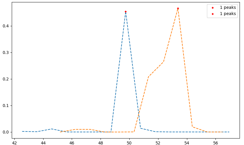
First, the data collected is aligned based on the timestamps attached to each sample. However, during our experiements, we noticed that the LiDAR data still suffer from a small delay. To synchronize the data further, we use a signal alignment technique based on the fact that integrating the accelerometer data once during a very small period of time guarantees that they will be no significant drift : We start by recording multiple 2 or 3 seconds of the IMU and LiDAR data where we try to produce a single spike by moving the IMU once in the field of view of the LiDAR. We then use the IMU data and LiDAR data to generate 2 velocity graphs and and use the spikes in both signals to align them. After calculating the delay value in all the recorded samples, we are able to calculate an average value of what the delay between the two sensors is, which is 3.89 ms. Fig. 1 shows one of the velocity plots used to calculate the delay average between the IMU and LiDAR.
V Stride Lengths Predictions
V-A Preparing and Segmenting the Data
We recorded the data in runs of 10 or 5 minutes. We always start by clipping the 3 first and last seconds of each run, which usually correspond to the periods when the subject was getting in or out of the frame of the LiDAR. We then proceed to normalize the data between and use a sliding window to segment it in sequences of 2 seconds each. After aligning the LiDAR and IMU data, we use the time stamps to assign two label dx and dy to each of the previously segmented sequences. The final data contained in the segmented sequences is a concatenation of the data generated by the triple-axis accelerometer, gyroscope, magnetometer and their magnitudes.
VI Neural Network
Our network structure consists of two stacked GRU layers [8] , followed by a drop out layer with a ratio of 0.25. We add on top of that an Attention layer [15] and finally 2 dense layers, with the last layer being the final regression one with a linear activation function. We used the same network architecture to predict both and . Both networks were implemented using Keras with a TensorFlow backend, and trained on an Nvidia Tesla K40. The networks were trained for 60 epochs, using a batch size of 5, the Mean Absolute Error (MAE) as a loss function and an RMSProp optimizer with a strarting learning rate of 0.001 that was decreased by a factor of 0.2 whenever the validation loss stopped improving for more than 10 epochs. The input dataset set was split into a training and validation datasets using a 0.8 split ratio. The testing dataset was not included in the input dataset. We also trained multiple variants of our network to prove the usefulness of the Attention layer. The other trained network (namely : Bilinear-LSTM [7], GRU, 2GRU, 3GRU) followed the same training procedure and used the same data.
Table 1 shows the order and details of the different layer that were used to build our Neural Network.
| Layer | Input | Output |
|---|---|---|
| (500,12) | (500,12) | |
| (500,12) | (500,256) | |
| (500,256) | (500,256) | |
| (500,256) | (500,256) | |
| (500,256) | (1,256) | |
| (1,256) | (1,64) | |
| (1,64) | (1) |
VII Results
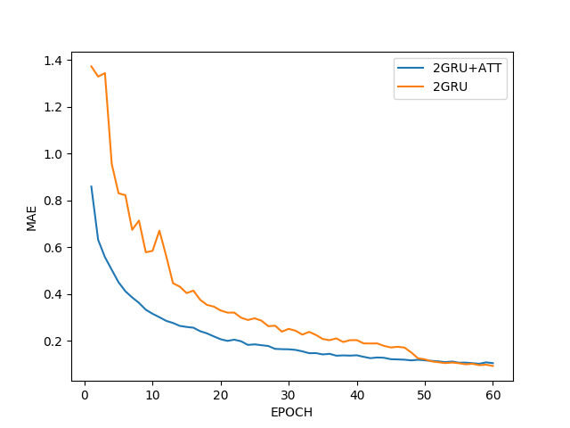
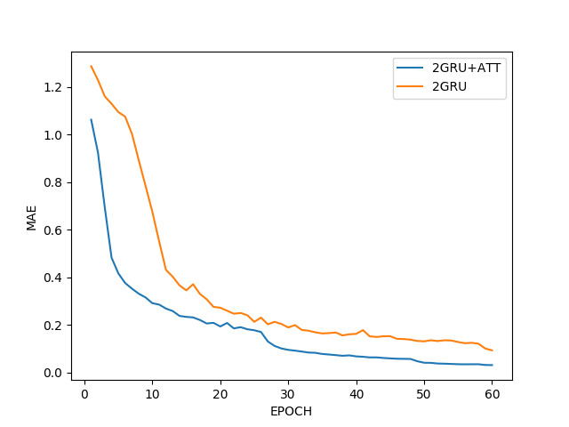
When it comes to predicitng SL for a freely moving human subject, our tests show that the proposed architecture outperforms any other variant or previously proposed network. Also the attention layer seems to make the training more stable and makes it converge faster. Our models are also very lightweight : only 8mb, and requires only 82ms to produce a prediction, making them ideal for real time deployment on embedded structures.
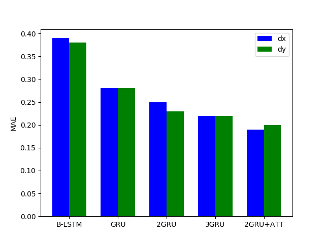
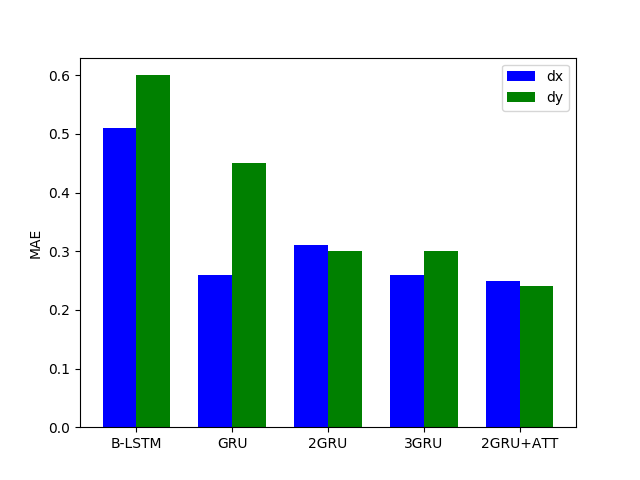
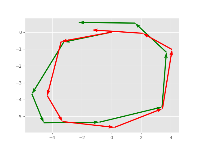
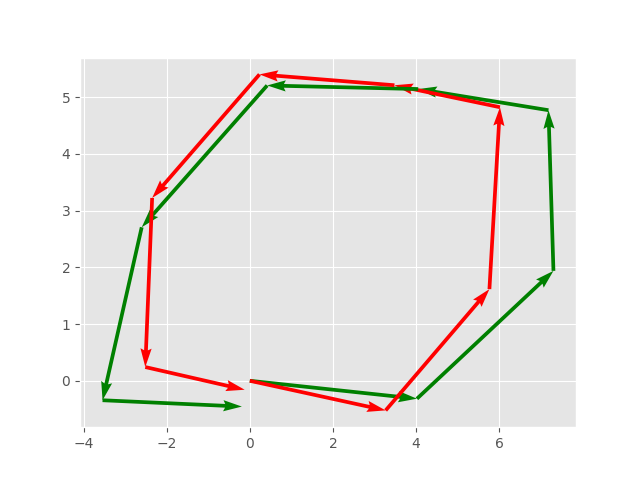
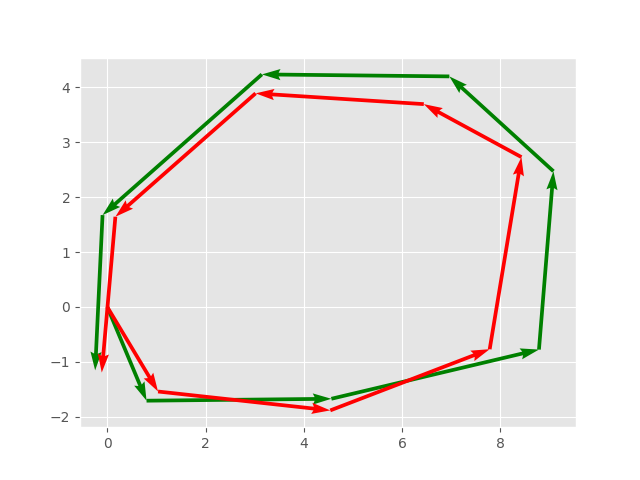
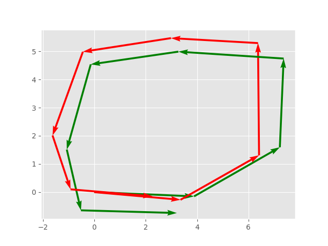
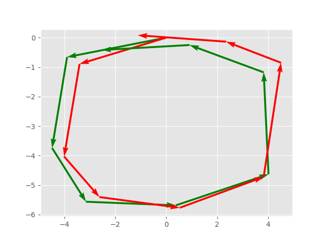
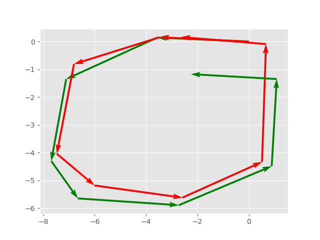
Fig. 2 and Fig. 3 list the different MAE scores of the different networks that were trained. Our method (2GRU+ATT) is shown to have the smallest final error value on both the test and validation datasets. Our final MAE for both the and models are and respectively for the validation dataset, and and respectively for the testing dataset. Fig. 3 shows a qualitative comparaison of some of the plots generated after feeding the test dataset to our trained network. We are able to reproduce the path followed by the subject by combining the predictions of both the dx and dy models.
Ablation Study : Fig. 5 and Fig. 6 show a comparison between the training plots of the NN with and without the Attention Layer for both the and networks. We can see that the Attention Layer helps the network to be more stable while learning and makes it converge faster.
VIII Conclusion
The initial experimental results shows the proposed method is promising. As more data are collected for training, the prediction model has the potential to become more accurate. In its present form, it provides good estimates of dx and dy displacement when the subject moves straight. But when the subject is turning, the predictions become less accurate. This is largely owing to the fact that the turning segments in our training dataset are disproportionally less than the straight movement. In the future work, we plan to collect more data and to generalize this approach to all typical motions such as walking, running, crawling, etc. The goal is to develop a generalized deep learning model that can track pedestrians even with complex motions.
References
- [1] S. Beauregard and H. Haas, “Pedestrian dead reckoning : A basis for personal positioning,” 2006.
- [2] S. Beauregard, “A helmet-mounted pedestrian dead reckoning system,” 2006.
- [3] A. R. Pratama, Widyawan, and R. Hidayat, “Smartphone-based pedestrian dead reckoning as an indoor positioning system,” 2012 International Conference on System Engineering and Technology (ICSET), pp. 1–6, 2012.
- [4] N. Kakiuchi and S. Kamijo, “Pedestrian dead reckoning for mobile phones through walking and running mode recognition,” 16th International IEEE Conference on Intelligent Transportation Systems (ITSC 2013), pp. 261–267, 2013.
- [5] A. A. Jiménez, F. P.-E. Seco, C. Prieto, and J. Guevara, “A comparison of pedestrian dead-reckoning algorithms using a low-cost mems imu,” 2009 IEEE International Symposium on Intelligent Signal Processing, pp. 37–42, 2009.
- [6] J. Hannink, T. Kautz, C. Pasluosta, J. Klucken, and B. Eskofier, “Sensor-based gait parameter extraction with deep convolutional neural networks,” IEEE Journal of Biomedical and Health Informatics, vol. PP, 09 2016.
- [7] M. Edel and E. Koppe, “An advanced method for pedestrian dead reckoning using blstm-rnns,” 2015 International Conference on Indoor Positioning and Indoor Navigation (IPIN), pp. 1–6, 2015.
- [8] J. Chung, Çaglar Gülçehre, K. Cho, and Y. Bengio, “Empirical evaluation of gated recurrent neural networks on sequence modeling,” ArXiv, vol. abs/1412.3555, 2014.
- [9] S. Hochreiter and J. Schmidhuber, “Long short-term memory,” Neural computation, vol. 9, no. 8, pp. 1735–1780, 1997.
- [10] A. Kumar, O. Irsoy, P. Ondruska, M. Iyyer, J. Bradbury, I. Gulrajani, V. Zhong, R. Paulus, and R. Socher, “Ask me anything: Dynamic memory networks for natural language processing,” ArXiv, vol. abs/1506.07285, 2015.
- [11] T. Bansal, D. Belanger, and A. McCallum, “Ask the gru: Multi-task learning for deep text recommendations,” ArXiv, vol. abs/1609.02116, 2016.
- [12] K. Xu, J. Ba, R. Kiros, K. Cho, A. C. Courville, R. Salakhutdinov, R. S. Zemel, and Y. Bengio, “Show, attend and tell: Neural image caption generation with visual attention,” in ICML, 2015.
- [13] A. Vaswani, N. Shazeer, N. Parmar, J. Uszkoreit, L. Jones, A. N. Gomez, L. u. Kaiser, and I. Polosukhin, “Attention is all you need,” in Advances in Neural Information Processing Systems 30, I. Guyon, U. V. Luxburg, S. Bengio, H. Wallach, R. Fergus, S. Vishwanathan, and R. Garnett, Eds. Curran Associates, Inc., 2017, pp. 5998–6008. [Online]. Available: http://papers.nips.cc/paper/7181-attention-is-all-you-need.pdf
- [14] J. K. Chorowski, D. Bahdanau, D. Serdyuk, K. Cho, and Y. Bengio, “Attention-based models for speech recognition,” in Advances in Neural Information Processing Systems 28, C. Cortes, N. D. Lawrence, D. D. Lee, M. Sugiyama, and R. Garnett, Eds. Curran Associates, Inc., 2015, pp. 577–585. [Online]. Available: http://papers.nips.cc/paper/5847-attention-based-models-for-speech-recognition.pdf
- [15] C. Raffel and D. P. W. Ellis, “Feed-forward networks with attention can solve some long-term memory problems,” ArXiv, vol. abs/1512.08756, 2015.