Spatial Variation in Strong Line Ratios and Physical Conditions in Two Strongly-Lensed Galaxies at z$\sim$1.4

Abstract

For studies of galaxy formation and evolution, one of the major benefits of the James Webb Space Telescope is that space-based IFUs like those on its NIRSpec and MIRI instruments will enable spatially resolved spectroscopy of distant galaxies, including spectroscopy at the scale of individual star-forming regions in galaxies that have been gravitationally lensed. In the meantime, there is only a very small subset of lensed sources where work like this is possible even with the Hubble Space Telescope’s Wide Field Camera 3 infrared channel grisms. We examine two of these sources, SDSS J1723$+$3411 and SDSS J2340$+$2947, using HST WFC3/IR grism data and supporting spatially-unresolved spectroscopy from several ground-based instruments to explore the size of spatial variations in observed strong emission line ratios like O32, R23, which are sensitive to ionization parameter and metallicity, and the Balmer decrement as an indicator of reddening. We find significant spatial variation in the reddening and the reddening-corrected O32 and R23 values which correspond to spreads of a few tenths of a dex in ionization parameter and metallicity. We also find clear evidence of a negative radial gradient in star formation in SDSS J2340$+$2947 and tentative evidence of one in SDSS J1723$+$3411  though its star formation is quite asymmetric. Finally, we find that reddening can vary enough spatially to make spatially-resolved reddening corrections necessary in order to characterize gradients in line ratios and the physical conditions inferred from them, necessitating the use of space-based IFUs for future work on larger, more statistically robust samples.

1. Introduction

Strong emission line ratios have emerged as powerful diagnostics to understand the physical conditions within distant (redshift $z\gtrsim 1$) galaxies, particularly the metallicity, pressure, and ionization state of the gas, and the amount of dust (e.g., Kewley & Dopita, 2002, Pettini & Pagel, 2004, Rigby et al., 2011, Steidel et al., 2014, Nakajima & Ouchi, 2014, among many others). Most observational studies that have used these diagnostics to characterize distant galaxies have, by necessity, used the integrated light of entire galaxies to measure them. However, a spatially–integrated measurement is unlikely to fairly represent all regions within a galaxy. Distant galaxies show kiloparsec-scale structures, called “giant clumps” (e.g., Elmegreen et al. 2005; Guo et al. 2012), though recent observational and theoretical results suggest that far smaller spatial scales—tens of parsecs rather than kiloparsecs—are important for star formation in the distant universe (Johnson et al., 2017; Mandelker et al., 2013). A spatially-integrated spectrum may well be dominated by the spectrum of one bright giant clump (or a single complex of smaller clumps), if it has extreme line ratios compared to the rest of the galaxy, particularly at bluer rest wavelengths. For instance, Girard et al. (2018) find that about 40% of the star formation, as indicated by H$\alpha$, lies in just three clumps in a lensed galaxy at $z=1.6$. Moving beyond a bulk measurement of galaxy spectra to truly understand the internal physics of these sources requires spectroscopic studies with high spatial resolution.

Surveys using integral field units have characterized how strong line ratios vary spatially in nearby galaxies. Metallicity gradients, for instance, have been observed in the local universe (e.g., Belfiore et al., 2017, Poetrodjojo et al., 2018), at low redshifts (e.g., $0.1\leq z\leq\ 0.8$ in Carton et al., 2018), and at moderate redshifts (e.g., lensed sources at $z=1.49$ and $2$ in Yuan et al., 2011 and Jones et al., 2010, respectively). Meanwhile, Poetrodjojo et al. (2018) have investigated, but did not find strong evidence of, radial gradients in ionization parameter at low redshifts, though other studies such as Ellison et al. (2018) have found evidence of radial gradients in star formation rate surface densities and Dopita et al. (2014) find correlations between SFR and ionization parameter.

While spatial variation of strong line diagnostics at subgalactic scales is well-established in low-redshift galaxies, it is not yet clear how these diagnostics vary spatially in more distant galaxies, which have systematically more extreme physical conditions (Kewley et al., 2015, Holden et al., 2016, Onodera et al., 2016) and far more disturbed morphologies in which giant clumpy structures are far more prevalent (Elmegreen et al., 2005, Shibuya et al., 2016). Furthermore, the star-formation histories of clumps in such young and disordered objects are likely much different than those of star-forming regions in the local universe. For example, the star-formation history of a single star-forming clump at $z\sim 1-3$ is more likely to be accurately described by a single stellar population than structures in older and more morphologically mature galaxies like the Milky Way would be since there has not been as much time for secondary bursts or mixing with older stellar populations from within the same galaxy or from mergers. It is therefore reasonable to suspect that in addition to more extreme physical conditions, higher redshift objects might also have more extreme variations in those conditions.

Additionally, the spatial variation of these diagnostics likely has important consequences for galaxy evolution and cosmology. For example, the strong line ratio O32 has been found to correlate with Lyman continuum (LyC) leakage (Nakajima et al., 2013; Izotov et al., 2018), likely due to its sensitivity to ionization parameter. But it is unclear whether this is a galaxy-wide phenomenon or a smaller more localized one. Izotov et al. (2018) and Nakajima et al. (2013) identify LyC leakage in the integrated light of their target galaxies, for example, but in a strongly lensed source, Rivera-Thorsen et al. (2019) finds LyC leakage from only a single clump. Understanding the details of processes like this will be critical to understanding how the universe became reionized.

Even with large space telescopes like the Hubble Space Telescope (HST) and the upcoming James Webb Space Telescope (JWST), diffraction limits prevent the study of spatial scales below $\sim 500$ pc in distant field galaxies. The exceptions are galaxies that have been highly magnified by gravitational lensing, thereby providing access to otherwise inaccessible spatial resolution. Lensing has enabled the measurement of star formation rates (Whitaker et al., 2014), metallicity gradients (Jones et al., 2010; Patricio et al., 2019), and rotation curves (Tiley et al., 2019; Wuyts et al., 2014) with tens of parsecs to a few hundred parsecs resolution for small numbers of galaxies.

In this Paper, we use HST grism spectroscopy from GO14230 (PI: Rigby) to measure the standard suite of rest-frame optical strong emission lines, from [O II] 3727, 3729Å to [S II] 6716, 6733Å, in two strongly lensed galaxies at z$\sim$1.4 selected from the Sloan Giant Arcs Survey (SGAS). We map the spatial variation of the diagnostic line ratios H$\alpha$/H$\beta$, R23, O32, and Ne3O2, which are sensitive to dust, metallicity, and ionization parameter. We quantify the spatial variation in these strong line ratios, and examine the corresponding variation in inferred physical characteristics of the nebular gas.

We also examine whether the spatially integrated spectra of these two galaxies tell the whole story of—or even accurately summarize—the physical properties of the nebular gas in the multiple distinct physical regions that are probed at lensing–boosted spatial resolution. Each of these objects provides an opportunity to see, directly, how much we miss by using integrated spectra. SDSS J2340$+$2947  at $z=1.42$, is lensed in such a way that there are 4 complete images of the source galaxy, each of which contains three distinct spatial regions from which we can obtain spectra. The other source, SDSS J1723$+$3411 at $z=1.33$, exists in a lensing configuration such that there are two partial (but nearly complete) images of the source combining to form a giant arc as well as two other magnified complete images and a central, demagnified complete image. The northern most complete image is well-enough separated from the BCG and intracluster light that its spectrum can also be extracted robustly from the HST grism spectroscopy for comparison.

This paper is organized as follows. § 2 describes the experimental design and sample selection. § 3 describes the broad-band imaging, HST spectroscopy, and ground-based spectroscopy that we have obtained to carry out this experiment. Details of emission line fitting are given in § 4. § 5 discusses the observed spatial variation of the strong emission line ratios, explores the implied corresponding variation in physical parameters, and compares the implied measurements for spatially integrated versus spatially resolved spectra. § 6 discusses the implications of such spatial variation in emission line ratios for studying galaxy evolution and the epoch of reionization, and discusses considerations for future observational and theoretical work.

2. Experimental Design and Sample Selection

This study requires technically demanding spectroscopy that fulfills three criteria. First, the highest possible spatial resolution is needed; this demands that the targets be gravitationally lensed, and further that they be observed either from space or with ground-based adaptive optics systems. Second, the spectra must have complete wavelength coverage from rest-frame 3727 Å (to cover the [O II] doublet) to 6730 Å (to cover the [S II] doublet). Third, the spectra must have excellent relative fluxing over that entire wavelength range, in order to use diagnostic line ratios. Together, these criteria drive the experiment to use the WFC3-IR grisms onboard HST. Of currently available spectrographs, only the WFC3-IR grisms provide high spatial resolution, excellent flux calibration, and uninterrupted wavelength coverage over this range.

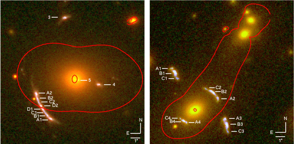
Figure 1.— Left: Three-color HST image (R: F160W, G:F775W, B:F390W) of SDSS J1723$+$3411 with critical curves plotted in red and labels of each image and region in white. Images 1 and 2 are incomplete images, with regions A–D appearing once in each half of the arc. Images 3, 4, and 5 are complete images. Image 3 is separated enough from the BCG that grism spectra could be extracted with minimal contamination. Right: Three-color HST image (R:F140W, G:F814W, B:F390W) of SDSS J2340$+$2947 with critical curves plotted in red and labels for each region in white. There are four complete images with three distinct physical regions that could be extracted from the grism spectroscopy in each. Lens models are described in section 5.1.

Used together, the G102 and G141 WFC3-IR grisms can cover the desired range of rest wavelength for galaxies in a narrow redshift range 1.15 $\lesssim z\lesssim$ 1.58. We therefore selected galaxies in this redshift range from SGAS. We required that the galaxies appear bright enough to obtain high-quality grism spectra, are highly magnified, and have lensing configurations that are amenable to modeling. Only two targets emerged from this selection: SDSS J1723$+$3411 (hereafter SGAS1723) with $z=1.3294\pm 0.0002$ (Kubo et al., 2010), and SDSS J2340$+$2947 (hereafter SGAS2340) with $z=1.420\pm 0.003$. SGAS1723 is one of the brightest lensed sources in the Sloan Digital Sky Survey (SDSS; York et al., 2000) footprint, and has been reported in several independent searches for lensed galaxies within that data (Kubo et al., 2010; Wen et al., 2011; Stark et al., 2013). SGAS2340 has not been previously reported. This lensing system was found as part of the SGAS visual examination of SDSS lines of sight with putative clusters or groups of galaxies, and confirmed as a lens using $gri$ imaging from the 2.5m Nordic Optical Telescope’s MOSCA instrument on UT 2012-09-16, with the lensed source then spectroscopically confirmed using the same telescope’s ALFOSC spectrograph on UT 2013-09-01.

To support the HST grism spectroscopy, we obtained ground-based spectroscopy from large ground-based telescopes. We obtained rest-frame ultraviolet (observed-frame optical) spectra with the Echellette Spectrograph and Imager (ESI) (Sheinis et al., 2002) on the Keck II telescope. We obtained rest-frame optical spectra of [N II] and H$\alpha$ with the Gemini Near-InfraRed Spectrograph (GNIRS) (Elias et al., 2006) on the Gemini-North telescope. These instruments provide much higher spectral resolution than the WFC3-IR grisms, but much lower spatial resolution since they are seeing-limited. Additionally, broadband imaging from HST and Spitzer were leveraged for the creation of lens models, interpretation of source morphologies, and the estimation of stellar masses of each source.

3. Observations, Data, and Data Reduction

Here we describe the observations, data, and data reduction for the spectra from Keck ESI, Gemini GNIRS, and the HST grisms as well as the broadband imaging from HST and Spitzer. All wavelengths are listed in vacuum. Source coordinates and redshifts are listed in Table 1 for ease of reference.

3.1. Broadband HST Imaging

We acquired broadband imaging for SGAS2340 and SGAS1723 using the Wide Field Camera 3 (WFC3) onboard HST, as needed to construct a lens model and do contamination modeling and wavelength calibrations for the grism data.

SGAS1723 was observed in six bands with HST WFC3: F160W, F140W, F110W, and F105W in the IR channel, and F775W and F390W in the UVIS channel. Imaging in the F160W and F110W bands was conducted as part of HST GO13003 (PI: Gladders) on 2013 March 14 for 1112 s each. Imaging with the UVIS channel in the F775W and F390W bands was conducted as part of the same program, with total integration times of 2380 s and 2368 s respectively. Imaging in the F140W and F105W bands was conducted as part of HST GO14230 (PI: Rigby) in January and July 2016 alongside the grism observations, for a total integration of 923 s per band.

SGAS2340 was observed in 4 bands with HST WFC3: F140W and F105W in the IR channel, paired with the grism observations, and F814W and F390W in the UVIS channel, all from program GO14230 (PI: Rigby). In the IR channel, SGAS2340 was observed with the F105W filter for 973 s and F140W for 1635 s; in the UVIS channel, it was observed with the F814W filter for 2504 s and F390W for 2600 s.

Source	RA (J2000)	Dec (J2000)	zgal	$\delta$ zgal
SGAS1723	17:23:36	+34:11:58	1.3293	0.0002
SGAS2340	23:40:29	+29:47:47	1.42151	0.00002

Table 1The positions and redshifts of the targets in this paper. Right ascensions and declinations (columns 2 and 3) are given in the J2000 coordinates and correspond to the centers of each lensing system (i.e., the BCG). Redshifts and uncertainties are for the lensed source galaxies and were determined by the GNIRS spectroscopy reported in this paper (§ 5.5).

For all HST broad-band imaging, a 4-point dither pattern was used. To reduce the imaging data, the images were aligned using the Drizzlepac routine tweakreg, and drizzled to a common refrence grid with a pixel scale of 0.03″ per pixel using astrodrizzle with a “drop size” (final_pixfrac) of 0.8. Three-color images of both SGAS1723 and SGAS2340 are shown in Fig. 1.

3.2. Broadband Spitzer Imaging

Data from the IRAC instrument of the Spitzer Space Telescope, acquired during the post-cryogenic “warm mission”, were obtained through program 90232 (for SGAS 1723; PI J. Rigby) and program 12001 (for SGAS 2340; PI J. Rigby). The individual frame times were 30 s; the total per-pixel integration times were 30 min in IRAC channel 1 (3.6 micron), and 10 min in IRAC channel 2 (4.5 micron). We processed the Spitzer IRAC Ch1 and Ch2 images as follows. At a high level, we followed the general guidance of the IRAC Cookbook for reducing the COSMOS medium-deep data, though with more stringent (3$\sigma$) outlier rejection, and with residual bias correction.

In more detail, we downloaded the “corrected basic calibrated data products” (cBCDs) from the Spitzer archive. These cBCDs are the exposure-level data that have been processed by the IRAC pipeline to remove instrumental signatures and artifacts, and to calibrate into physical units. We applied the warm mission column pulldown correction (bandcor_warm by Matt Ashby) to mitigate column artifacts from bright sources.

For deep integrations, residual bias pattern noise and persistence can dominate over the background. To mitigate these effects, we constructed images of the residual bias, also known as a “delta dark frame”. For each channel in each observation, we created a residual bias correction from all the cBCDs, by detecting and masking sources in each image, adjusting the DC level of each image so that the modes had the same value, and then taking the median with 3$\sigma$ outlier rejection. The relevant median image was then subtracted from every cBCD image in that channel and that observation.

For each target and each filter, we combined the individual images into a mosaic as follows using the mopex command-line tools. We used the overlap correct tool to add an additive correction for each residual-bias–corrected cBCD image to bring it to a common sky background level. We then combined these images into a mosaic using the mopex mosaic tool, using the drizzle algorithm with a pixel fraction of 0.6, and 3$\sigma$ outlier rejection using the box outlier rejection method.

3.3. Keck ESI spectroscopy

Both galaxies were observed with the ESI spectrograph on the Keck II telescope on the nights of 2016 August 27 and 28 UT. Observing time was obtained through the Australian National University. Figure 2 shows how slits were oriented for observations of SGAS2340. A similar figure showing slit orientations for observations of SGAS1723 appears in Rigby et al. (in prep). SGAS1723 was observed each night, with a slit placed along the length of the arc, for 3600 s the first night and 3800 s the second night. For SGAS2340, each of the four complete images were observed each night with the following strategy. Images 1 and 2 were observed simultaneously, for 3800 s on the first night and 3600 s on the second night. Images 3 and 4 were observed simultaneously, for 3600 s on each night. Light from all three spatial subregions of SGAS2340 was captured by the slit.

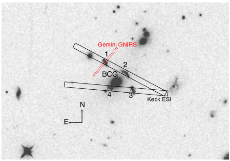
Figure 2.— Finderchart to show spectroscopic slit positions for the lensed galaxy SDSS J2340$+$2947. The background image is HST WFC3-IR F105W. The long rectangles show the two Keck ESI pointings (with a 1 by 20″ long slit), which each captured a pair of images of the lensed galaxy: 1 and 2 in one slit, 3 and 4 in the other. The red rectangle shows the Gemini GNIRS pointing, with a 0.3 by 7″ slit. The ESI slits were positioned by offsetting from the BCG, which is also marked. North and East are shown with a compass.

We reduced the Keck ESI spectra following the same procedure as Rigby et al. 2020 (in prep). For SGAS2340, we extracted the spectrum of each image individually. Line ratios are measured from the sum of the four images’ spectra.

3.3.1 Gemini GNIRS spectroscopy

Gemini GNIRS observations of SGAS1723 and SGAS2340 were obtained through the Gemini Fast Turnaround mode in program GN-2016B-FT-11 (PI Rigby). Observations were conducted on UT 2016-09-07. Observations used the short camera, cross-dispersing prism (“SXD” mode), 0.3″ slit, and the 111 lines/mm grating. Data were obtained as A–B nods. For SGAS1723 the central wavelength was set to 1.529 $\mu$m; for SGAS2340 it was set to 1.588 $\mu$m. Figure 2 shows where the GNIRS slit was positioned for SGAS2340. A similar figure for SGAS1723 is available in Rigby et al.(in prep). For SGAS1723  the GNIRS slit primarily captured light from the brightest region in the southern part of the arc, region A1. For SGAS2340  the GNIRS slit primarily captured light from the central region, “B”. For SGAS1723, the cumulative integration time (discarding one exposure with data quality issues) was 2970 s. For SGAS2340, 12 integrations of 270 s duration were obtained, for a total integration time of 3240 s.

The GNIRS spectra were reduced in IRAF using the GNIRS pipeline, which does sky subtraction by differencing A–B pairs. From each A–B pair, spectra of the A and B images were extracted using a 7 pixel wide boxcar. We combined the individual spectra by calculating the mean spectrum and the error in the mean. Rigby et al. (in prep) discuss special care that had to be taken with the reduction for SGAS1723, due to the fact that the grating shifted position during the observations.

3.4. HST grism spectroscopy

Spectroscopy for SGAS1723 and SGAS2340 was conducted using the HST WFC3/IR G141 and G102 grisms alongside the direct imaging from program GO14230 described in section 3.1.

At the redshift of these arcs, z$\sim$1.4, these grism observations cover the wavelength range from just blueward of [O II] 3727, 3729 Å to just redward of H$\alpha$. Each target was observed twice with each grism, using two different roll angles to facilitate the modeling of contamination from cluster galaxies. For SGAS1723, observations in each grism were performed for 5112 s at one roll angle, and 4812 s at the other. SGAS2340 was observed with a similar strategy except that the exposure times were 7518 s for both roll angles with the G141 grism, and 5012 and 5112 s for the two roll angles with the G102 grism.

The HST grism spectra were reduced with the software package Grizli. We followed the standard Grizli reduction pipeline steps, with a notable extra step of GALFIT (Peng et al., 2010) modeling to account for the contaminating light of the cluster galaxies. This extra step is described in detail in Rigby et al. (in prep), and was performed on the grism data for both targets.

In this paper, we separately extract the HST grism spectra of physically distinct regions within each of the lensed galaxies, guided by the source-plane morphologies described in § 5.2. (This is in contrast to the approach of Rigby et al. (in prep), which considers only the spatially-integrated 1D spectrum of the giant arc of SGAS1723). These regions are labeled with letters in Fig. 1. The 1D spectrum of each individual subregion was constructed by summing over the relevant rows in the 2D grism spectrum, and then stacking the spectra of the multiple lensed images of that region. When the lensing geometry and orientation relative to the dispersion axis of the grisms allows for low morphological broadening and little to no spectral contamination from other pieces of the arcs, spectra from both roll angles are also summed.

For SGAS1723 we separately extract the HST grism spectra for the three clumps (A, B, D) and a diffuse component of the giant arc (C), each of which are imaged twice (A1, A2; B1, B2; etc.), and additionally extract the spectrum of the northern complete image (image 3).

For SGAS2340 we separately extract the HST grism spectra for the following physically-distinct regions. For region A, we extract a spectrum from three of the four lensed images at one roll, and one of the images at the other roll. For region B, we extract a spectrum from three images at one roll, and two images at the other. For region C, we extract a spectrum from two images at each roll (one image at both rolls, and two other images at one roll each). These decisions were guided by the quality of the grism contamination models and the orientation of each image relative to the dispersion axis. The spectra of each region were stacked over the multiple images and rolls. Table 2 summarizes which spectra were included in each of these stacks.

The grism spectra were corrected for foreground reddening from the Milky Way galaxy using the $E(B-V)$ values measured by Green et al. (2015).

Region	Images From Roll 1	Images From Roll 2
A	A1, A2, A4	A1
B	B1, B2, B4	B1, B4
C	C2	C1, C2, C3
Complete Image	1, 2, 4	1

Table 2Images included in the stacked spectra for each region of SDSS J2340$+$2947. Names correspond to the labels in Fig. 1

4. Data Analysis Methods

4.1. Fitting emission lines in the Keck ESI spectra

We fit emission lines in the ESI spectra using the continuum and emission line fitting routines described in Acharyya et al. (2019).

4.2. Fitting emission lines in the Gemini GNIRS spectra

We fit the spectra with Gaussians using MPFIT, as described in Wuyts et al. (2014). The uncertainty spectrum was used as weights in the fitting. The central wavelengths of all lines were set using the rest wavelength from NIST and the measured H$\alpha$ redshift. The widths of all lines were forced to vary in lockstep. The flux ratio of the [N II] doublet was locked at the value from Storey & Zeippen (2000).

4.3. Fitting emission lines in the HST grism spectra

Line fluxes were measured from the stacked spectra using the custom fitting technique described in Rigby et al. (in prep), with a few minor changes to compensate for the lower signal-to-noise ratios of the spectra of individual regions, compared to the spatially–integrated spectrum of the giant arc studied in that paper. Two iterations of the fitting algorithm were run on each spectrum. The first iteration solves for the redshift, the morphological line broadening (a nuisance parameter), and the line fluxes and uncertainties. The second iteration fixes the redshift and morphological broadening parameter determined in the first iteration, and then allows for small variations in the observed wavelength of each emission feature; this is motivated by known uncertainties in the wavelength solutions of HST grism spectra. The second iteration typically resulted in better overall spectral fits. However, for a few low signal-to-noise spectra (the integrated spectra of images 1, 2, and 3 of SGAS2340 from the G102 grism), the second iteration resulted in poorer fits; for those spectra we report only the line fluxes measured from the first iteration.

At the low spectral resolution of the WFC3/IR grisms, the [N II] doublet is unrecoverably blended with H$\alpha$. Therefore, we set the [N II] doublet ratio to its theoretical value (Storey & Zeippen, 2000), and set the [N II]/H$\alpha$ ratio to the value measured from the spatially–integrated Gemini GNIRS spectrum of each galaxy (see §5.5). Similarly, the [O II] 3727/3729 flux ratio was set to the value measured from the Keck ESI spectra (§ 5.4). These values were used for all physical regions of SGAS1723 and SGAS2340 despite coming from the integrated spectrum.

5. Results

5.1. Lens Models

We used the strong lensing evidence, i.e., identification of multiply-imaged lensed galaxies, in order to compute strong lensing models for SGAS1723 and SGAS2340. The lensing analysis of SGAS1723 was published in Sharon et al. (2020) as part of the SGAS-HST program. We describe here the lensing analysis of SGAS2340. However, we note that the lensing analysis of both clusters follows the same procedure.

We identified two strongly lensed galaxies in this field. Source 1, the topic of this paper, has four complete images around the core of the cluster. The images are resolved and show identical morphology and color variation. We used the central positions of four distinct morphological features in each image, as well as the spectroscopic redshift of the source galaxy, $z_{spec}=1.42$, as lensing constraints. Source 2 appears as three images of a faint galaxy, $6\farcs 44$ northwest of the BCG. Its redshift is unknown, and was used as a free parameter in the lens modeling process. Constraints are tabulated in Table 3

The lens model was computed using the publicly available software Lenstool (Jullo et al., 2007). Lenstool uses a bayesian approach to explore the parameter space and identify the best-fit model, as the set of parameters that minimize the scatter between the predicted and observed lensed images in the image plane. The lens model results in a parametric two dimensional description of the lens plane, from which the projected mass density, lensing magnification, and deflection are derived.

The lens was modeled as a linear combination of parameterized mass halos. Each halo was assumed to be a Pseudo Isothermal Elliptical Mass Distribution (PIEMD, or dPIE; Elíasdóttir et al., 2007), with the following parameters: position $x$, $y$; ellipticity $e$; position angle $\theta$; core radius $r_{c}$; truncation radius $r_{cut}$, and normalization $\sigma_{0}$. The lens is composed of cluster-scale halos and galaxy-scale halos. The latter were placed at the positions of observed cluster-member galaxies, identified using the red sequence technique (Gladders & Yee, 2000) in the F814W-F105W color-magnitude space. The position, ellipticity, and position angle of the galaxy halos were fixed to their observed values as measured with Source Extractor (Bertin & Arnouts, 1996). The other parameters are scaled to the luminosity, following Limousin et al. (2005). All the parameters of cluster-scale halos were left free, except for $r_{cut}$ which is beyond the range that can be constrained by the lensing evidence. It was fixed to 1500 kpc.

We find that the lens is best described by two cluster/group scale halos, combined with galaxy scale halos. The statistical uncertainties were derived by computing the lensing outputs from sets of parameters drawn from steps in the MCMC chain. Magnifications and the corresponding uncertainties are tabulated for both this source and SGAS1723 in Table 4. The relatively small number of lensed galaxies in this field limited the number of constraints available for lens modeling, resulting in more uncertain models and relatively larger statistical uncertainties in magnification than for SGAS1723.

ID	R.A.	Decl.	$z_{spec}$	$z_{model}$
	(J2000)	(J2000)
A1	355.119674	29.797717
A2	355.118160	29.796868
A3	355.117915	29.796249
A4	355.119201	29.796155
B1a	355.119622	29.797621	1.4200
B2a	355.118294	29.796994
B3a	355.117874	29.796099
B4a	355.119274	29.796182
B1b	355.119573	29.797569
B2b	355.118377	29.797054
B3b	355.117848	29.796033
B4b	355.119316	29.796206
C1	355.119524	29.797421
C2	355.118555	29.797102
C3	355.117837	29.795886
C4	355.119419	29.796267
11.1	355.118291	29.798323		$1.34^{+0.68}_{-0.42}$
11.2	355.117948	29.798055
11.3	355.117203	29.797563

Table 3Lensing constraints used in the lens model of SDSS J2340$+$2947. IDs correspond to labels in Fig.  1. Region B has been broken up into two components (labeled with lowercase a and b) for modeling. B1a is the northern half of region B in image 1. B2a is the southern half of region B in image 1. IDs beginning with “11” correspond to a second source not studied in this paper.

Source	Region	Magnification	$m_{160}$	$m_{140}$	$m_{110}$	$m_{105}$	$m_{814}$	$m_{775}$	$m_{390}$	$fH\beta\ _{obs}$	$\delta\ fH\beta\ _{obs}$
1723+3411	A1	$16.4^{+0.5}_{-1.4}$	21.8	21.9	21.9	21.5	–	22.3	22.4	15.81	0.75
1723+3411	A2	$16.6^{+0.5}_{-1.6}$	21.9	22.1	22.0	21.7	–	22.4	22.6	18.81	0.63
1723+3411	B1	$25.0^{+0.9}_{-2.1}$	22.6	22.4	22.8	22.2	–	22.9	22.9	7.01	0.35
1723+3411	B2	$25.9^{+0.9}_{-2.3}$	22.5	22.5	22.5	22.2	–	22.9	23.0	7.07	035
1723+3411	C1	$36.2^{+0.9}_{-3.3}$	23.1	23.0	23.3	22.8	–	23.3	23.3	4.76	0.35
1723+3411	C2	$40.3^{+1.4}_{-3.6}$	23.3	23.2	23.4	23.0	–	23.7	23.6	6.32	0.46
1723+3411	D1	$102.7^{+8.2}_{-8.5}$	22.2	22.3	22.4	22.2	–	22.7	23.0	5.29	0.47
1723+3411	D2	$112.6^{+7.6}_{-10.1}$	22.3	22.2	22.4	22.2	–	22.6	22.9	4.78	0.43
1723+3411	Giant Arc	$52.7^{+3.3}_{-1.2}$	20.1	20.2	20.2	19.9	–	20.5	20.6	71.14	2.09
1723+3411	Complete Image 3	$7.2_{-0.31}^{+0.33}$	22.0	22.1	22.0	21.8	–	22.5	23.6	10.72	0.90
2340+2947	A1	$8.9^{+9.0}_{-2.2}$	–	23.3	–	23.8	23.8	–	25.1	6.50	0.45
2340+2947	A2	$8.5^{+8.3}_{-1.7}$	–	22.9	–	23.4	23.4	–	24.4	9.49	0.65
2340+2947	A3	$12.8^{+12.2}_{-3.2}$	–	22.7	–	23.2	23.2	–	24.1	12.47	0.86
2340+2947	A4	$3.1^{+3.0}_{-0.7}$	–	23.5	–	24.0	24.1	–	25.2	3.94	0.27
2340+2947	B1	$9.8^{+10.0}_{-2.2}$	–	22.1	–	22.4	22.5	–	23.3	15.51	0.95
2340+2947	B2	$6.5^{+6.4}_{-1.5}$	–	22.2	–	22.5	22.6	–	23.5	12.72	0.78
2340+2947	B3	$9.2^{+8.1}_{-2.3}$	–	22.1	–	22.4	22.5	–	23.3	15.04	0.92
2340+2947	B4	$2.8^{+2.5}_{-0.6}$	–	22.8	–	23.2	23.3	–	24.3	5.82	0.36
2340+2947	C1	$11.4^{+11.3}_{-2.5}$	–	23.6	–	23.8	24.0	–	24.7	7.85	0.68
2340+2947	C2	$6.8^{+6.9}_{-1.7}$	–	23.5	–	23.9	24.1	–	25.1	5.57	0.48
2340+2947	C3	$7.6^{+7.0}_{-1.8}$	–	23.8	–	24.2	24.3	–	25.0	5.81	0.50
2340+2947	C4	$3.2^{+2.7}_{-0.7}$	–	24.4	–	24.8	25.0	–	26.1	2.16	0.19
2340+2947	Complete Image 1	$9.9^{+9.9}_{-2.3}$	–	21.6	–	22.0	22.0	–	22.9	30.60	1.77
2340+2947	Complete Image 2	$7.1^{+7.0}_{-1.6}$	–	21.6	–	21.9	22.0	–	22.9	27.72	1.61
2340+2947	Complete Image 3	$9.7^{+8.5}_{-2.4}$	–	21.5	–	21.8	21.9	–	22.7	33.24	1.93
2340+2947	Complete Image 4	$3.0^{+2.7}_{-0.7}$	–	22.2	–	22.6	22.7	–	23.8	12.13	0.70

Table 4Magnifications, magnitudes, and H$\beta$ fluxes of each of the images and subregions of SGAS1723 and SGAS2340. Columns 1 and 2 denote the source and the image or subregion. Column 3 contains the magnifications of each region and each complete image of SGAS1723 and SGAS2340. Uncertainties are reported as the 68% level. e.g., for SGAS1723 region A1, 68% of models that produce magnifications below 16.6 produce magnifications above 15.0 and 68% of models that produce magnifications larger than 16.6 produce magnifications below 17.1. Columns 4-10 contain the magnitudes of each region or complete image obtained from simple aperture photometry in each of the available HST filters. For the purposes of planning future observations, the observed H$\beta$ flux is included for each component in column 11 with its uncertainty in column 12. Rather than reporting line fluxes based on fits of individual, often low S/N spectra, we report values measured from the stacked spectra of all images of each region, scaled based on the number of roll angles and the flux ratios from the broadband imaging. The flux ratios used for scaling here are determined from the stacks of the imaging data in the UVIS channel because the higher spatial resolution allows better separation of the subregions while the flux ratios are consistent regardless of wavelength. A full list of fluxes, scaled to H$\beta$ is available as a machine-readable table.

5.2. Source Morphologies

The lens models enable a reconstruction of the source-plane morphology, which informs our extraction and summation of the HST grism data.

The giant arc in SGAS1723 is a merging pair of images of a single source galaxy. Each of these images is nearly complete. As Figure 1 shows, six large clumps are apparent in the broadband imaging; these are two images of each of the three physically distinct clumps (A, B, and D). An additional region, labeled C, appears to correspond to either a diffuse component, or to multiple spatially un-resolved clumps. In addition to the giant arc in SGAS1723, there are two complete but less magnified images of the lensed galaxy (images 3 and 4) and a demagnified central image (5). The grism spectra of images 4 and 5 are badly contaminated by the BCG; we were, howerver, able to extract the spectrum of the northern complete image (3).

There are four lensed images of the source galaxy SGAS2340. Each features a bright central region (B) and two fainter clumps near the edges (A and C). All of these regions, for both sources, are labeled in Figure 1 and correspond to the regions from which the spectra described in § 3.4 were extracted. Because the dither pattern of the HST imaging observations allows us to oversample the PSF, our final drizzled data products are able to resolve region B into two sub-components for the purposes of lens modeling. However, drizzling spectra produces correlated noise which can mimic emission or absorption features, so we are forced to use coarser pixels for the spectral data and interlace rather than drizzle, which reduces the effective spatial resolution of the spectral data and blends the spectra of the two sub-components of region B.

To summarize, for SGAS1723 we extract spectra of four physically distinct regions as well as one complete image; for SGAS2340 we extract spectra of three regions and also create a stacked composite spectrum of the complete images.

5.3. Photometry from the HST images

Broadband magnitudes for SGAS2340 and the giant arc in SGAS1723 were determined using a GALFIT decomposition of each source galaxy. Using these integrated magnitudes, magnitudes measured from the Spitzer data, the magnifications in Table 4 and the stellar population synthesis parameter inference code, Prospector (Leja et al., 2017), we estimated stellar masses of $9.67^{+9.0}_{-4.4}\times 10^{8}$ M_⊙ for the source in SGAS2340 and $5.95^{+2.2}_{-1.86}\times 10^{8}$ M_⊙ for SGAS1723 . Details of these measurements and the process used to infer the stellar masses are included in the Appendix. For the purposes of planning future observations, approximate apparent magnitudes (uncorrected for lensing magnification) of each individual region in these images based on photometry from custom apertures are included, along with the magnifications, in Table 4. We also include the estimated H$\beta$ flux for each region determined by correcting the H$\beta$ flux from the stacked spectrum using the observed broadband flux ratios of the various images of each region.

5.4. Keck ESI results

Fluxes for emission lines measured from the ESI spectra for SGAS1723 are listed in Table 1 of Rigby et al. (in prep), and for SGAS2340 are listed in Table 5 of this paper.

For SGAS1723, the [O II] 3727/3729 flux ratio was measured as $0.71\pm 0.01$. For SGAS2340, the [O II] 3727/3729 flux ratio was measured as $0.82\pm 0.01$.

These values are measured from spatially integrated spectra. Because the HST grisms do not spectrally resolve this doublet, the pressures assumed in section 5.8.2 are based on these values.

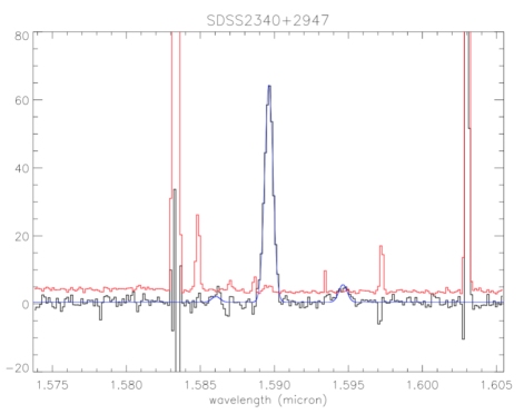
Figure 3.— The $\alpha$ and the [N II] doublet in the Gemini GNIRS spectrum of SGAS2340. Black steps show the summed one-dimensional spectrum; red steps show the uncertainty spectrum, and the blue curve shows the best fit.

5.5. GNIRS Gemini results

For SGAS1723, results from the Gemini GNIRS spectrum were presented in Rigby et al. (in prep). The redshift was measured as $z(H\alpha)=1.3293\pm 0.0002$. The [N II] 6586 / H$\alpha$ flux ratio was measured to be $0.062\pm 0.011$.

For SGAS2340, we measure the redshift of H$\alpha$ as $z=1.42151\pm 0.00002$ . The [N II] 6586 / H$\alpha$ flux ratio is measured to be $0.084\pm 0.03$ (Fig. 3).

These values are spatially integrated for SGAS2340 and come from clump A1 in SGAS1723 .

5.6. Line flux measurements from the HST grism spectra

An example of a reduced 2D grism spectrum for a single image of SGAS2340 and the 1D extraction and linefitting for each subregion is shown in Fig 4. Line fluxes for the stacks of each region in SGAS1723 and SGAS2340 normalized to the H$\beta$ flux, as well as line fluxes for each individual image of each region normalized to the H$\beta$ flux are included as machine readable tables in the electronic version of this article. These are included with the understanding that they may be needed for planning future observations and therefore the H$\beta$ fluxes are reported as observed, not corrected for the lensing magnification. Corrections can be made using the information in Table 4.

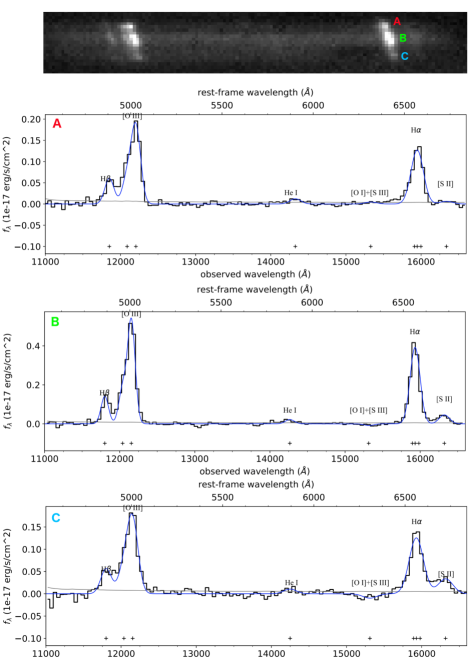
Figure 4.— An example of a reduced 2D grism spectrum (top) for SGAS2340 and the extracted 1D spectra for each of three regions labeled A (second from top), B (second from bottom), and C (bottom), corresponding to the labels in Fig. 1. The 1D continuum-subtracted spectrum is plotted in black, with the fit in blue. The continuum fit is plotted in grey. Emission lines are labeled and their best-fit wavelengths are marked by crosses. This example uses the G141 grism.

5.7. Spatial variation of strong line diagnostics

We investigate the spatial variation of several strong line diagnostics sensitive to dust, ionization parameter, metallicity and star formation rate. Of these, only the H$\alpha$ flux, a star formation rate indicator, is sensitive to the magnification due to gravitational lensing. The others, because they are flux ratios rather than fluxes, are invariant under lensing. Here, we describe the degree of variation seen in observables—line fluxes and ratios. In § 5.8 we explore how these variations correspond to variation in physical parameters, namely metallicity and ionization parameter.

5.7.1 Ratios Sensitive to Reddening: H$\alpha$/H$\beta$ and H$\beta$/H$\gamma$

We use Balmer decrements to estimate the reddening at each region within these two sources. For SGAS1723, H$\alpha$ falls in G141, H$\gamma$ falls in G102, and H$\beta$ is covered by both grisms. We find that H$\beta$ fluxes measured in G102 are more consistent from roll-to-roll than those measured from G141; we attribute this to H$\beta$ falling at an observed wavelength where the sensitivity of the G141 grism is rapidly declining. For SGAS2340, H$\alpha$ and H$\beta$ are both captured by the G141 grism, while H$\gamma$ is captured by G102.

Fig. 5 shows the measured H$\alpha$/H$\beta$ flux ratios. From these, we infer E(B-V) reddening values assuming case B recombination.

Line ID	$\lambda_{\mathrm{rest}}$	Wr,fit	$\delta$ Wr,fit	Wr,signi	fluxobs	$\delta$ fluxobs
	(Å)	(Å)	(Å)	(Å)	(10-17 ergs/s/cm2)	(10-17 ergs/s/cm2)
O III] 1660	1660.8090	-3.05	1.86	4.17	28.6	17.39
O III] 1666	1666.1500	$>$-2.04	..	..	$<$8.38	..
N III] 1750	1749.7000	$>$-0.77	..	..	$<$7.97	..
[Si II] 1808	1808.0130	$>$-4.29	..	..	$<$44.4	..
[Si II] 1816	1816.9280	$>$-36.6	..	..	$<$376.	..
[Si III] 1882	1882.7070	$>$-0.37	..	..	$<$3.13	..
Si III] 1892	1892.0290	$>$-0.33	..	..	$<$2.72	..
[C III] 1906	1906.6800	$>$-0.30	..	..	$<$2.46	..
C III] 1908	1908.7300	$>$-0.29	..	..	$<$2.37	..
N II] 2140	2139.6800	$>$-0.37	..	..	$<$0.69	..
[O III] 2320	2321.6640	$>$-0.33	..	..	$<$0.59	..
C II] 2323	2324.2140	$>$-0.33	..	..	$<$0.60	..
C II] 2325c	2326.1130	-0.98	0.44	8.81	4.28	1.92
C II] 2325d	2327.6450	$>$-0.32	..	..	$<$0.58	..
C II] 2328	2328.8380	$>$-0.33	..	..	$<$0.59	..
Si II] 2335a	2335.1230	$>$-0.32	..	..	$<$0.58	..
Si II] 2335b	2335.3210	$>$-0.33	..	..	$<$0.59	..
Fe II 2365	2365.5520	-0.45	0.22	3.54	1.96	0.98
Fe II 2396a	2396.1497	$>$-0.49	..	..	$<$0.89	..
Fe II 2396b	2396.3559	$>$-0.49	..	..	$<$0.89	..
[O II] 2470	2471.0270	-0.52	0.22	3.46	2.19	0.92
Fe II 2599	2599.1465	$>$-0.34	..	..	$<$0.56	..
Fe II 2607	2607.8664	$>$-0.38	..	..	$<$0.63	..
Fe II 2612	2612.6542	$>$-0.40	..	..	$<$0.65	..
Fe II 2614	2614.6051	$>$-0.47	..	..	$<$0.77	..
Fe II 2618	2618.3991	$>$-0.43	..	..	$<$0.69	..
Fe II 2621	2621.1912	$>$-0.41	..	..	$<$0.67	..
Fe II 2622	2622.4518	$>$-0.49	..	..	$<$0.8	..
Fe II 2626	2626.4511	-0.65	0.21	4.33	2.56	0.84
Fe II 2629	2629.0777	$>$-0.62	..	..	$<$1.01	..
Fe II 2631	2631.8321	$>$-0.47	..	..	$<$0.76	..
Fe II 2632	2632.1081	$>$-0.46	..	..	$<$0.75	..
Mg II 2797b	2798.7550	-1.40	0.15	13.8	5.33	0.57
Mg II 2797d	2803.5310	-0.85	0.15	7.96	3.25	0.57
He I 2945	2945.1030	$>$-0.47	..	..	$<$0.73	..
He I 3187	3188.6660	$>$-0.41	..	..	$<$0.61	..
Ti II 3239	3239.9712	$>$-0.34	..	..	$<$0.50	..
Ne III 3342	3343.1420	$>$-0.61	..	..	$<$0.93	..
S III 3721	3722.6870	$>$-0.35	..	..	$<$0.48	..
[O II] 3727	3727.0920	-20.6	0.26	146.	68.8	0.85
[O II] 3729	3729.9000	-25.1	0.25	164.	83.5	0.83
H$\eta$	3836.4790	-0.62	0.25	3.04	2.22	0.89
[Ne III] 3869	3869.8610	-3.97	0.64	8.07	14.2	2.28
H$\zeta$	3890.1580	-3.57	0.81	9.11	12.8	2.91

Table 5Keck ESI line flux measurements for SDSS J2340$+$2947. The reported numbers are measured from the summed spectra of the four images. Images 2, 3 and 4 are 0.91, 1.09, and 0.40 times as bright, respectively, as image 1. flux_obs and $\delta$ flux_obs denote the observed flux and uncertainty respectively. W_r,fit and $\delta$ W_r,fit denote the rest-frame equivalent width measured and the corresponding uncertainty in Å  respectively, with negative values indicating emission (rather than absorption) lines. For cases of non-detection (i.e. $<$3 $\sigma$ detection), the 3$\sigma$ upper limit on equivalent widths and fluxes are quoted.

SGAS1723 does not appear to be substantially reddened at any location. Region C is consistent with an $E(B-V)$ of zero, though the $1\sigma$ measurement uncertainties in the H_α and H_β lines allow $E(B-V)$to be as high as 0.07. The region with the most reddening is region B, with E(B-V) $=$ 0.10 $\pm$ 0.05. Regions A and D fall in between these values, with reddenings of 0.02 $\pm$ 0.05 and 0.04 $\pm$ 0.09 respectively, though like region C, they are both consistent with zero. There is little evidence of spatial variation in reddening in SGAS1723 except that region B may be slightly more reddened than the other regions as it is the only region inconsistent with zero reddening at about the 2$\sigma$ level.

SGAS2340 shows signs of strong variation in the Balmer line ratios. Regions A and B are more reddened than any of the regions in SGAS1723, having E(B-V) $=$ 0.39 $\pm$ 0.07 and 0.38 $\pm$ 0.06 respectively. Region C, however, is notably less reddened, with E(B-V) $=$ 0.06 $\pm$ 0.13, which is consistent with zero and more comparable to SGAS1723 than to the other regions within SGAS2340. The H$\alpha$/H$\beta$ ratio for region C differs from those of regions A and B by about 2.8$\sigma$. Of the three regions within SGAS2340, region C appears the bluest in broadband imaging, which is consistent with this apparent lower level of extinction, but could also be due, for example, to lower metallicities or a younger stellar population.

In principle, reddening can also be determined using the H$\beta$/H$\gamma$ ratio. In practice, the smaller wavelength separation relative to H$\alpha$/H$\beta$ and the relative faintness of H$\gamma$ make it less useful than H$\alpha$/H$\beta$. In addition, at the low spectral resolution of the G102 grism, H$\gamma$ is blended with [O III] 4363Å, which is responsible for the high uncertainties in our quoted H$\gamma$ flux. We find that, in these spectra, the uncertainties on the H$\gamma$ flux prevent a meaningful measurement of the reddening via H$\beta$/H$\gamma$.

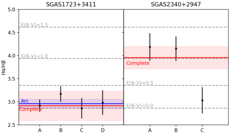
Figure 5.— The H$\alpha$ to H$\beta$ ratios in SGAS1723 (left) and SGAS2340 (right). The latter shows significant spatial variation, with region C being uniquely low. The spatial variation in SGAS1723 is less pronounced, though the difference between region B and region C is suggestive (but not statistically significant). The red bands in each plot show the spatially integrated values measured from the stack of the complete images of SGAS2340, and from the northern complete image of SGAS1723; the widths of the bands correspond to the uncertainties. In blue bands we show the values measured from the integrated spectrum of the giant arc in SGAS1723. For reference, several values of $E(B-V)$for case B recombination and R_v=3.1 are shown by gray dashed lines. While all of the H_α/H_β values are in general agreement for SGAS1723, it is clear that the value inferred from the integrated spectrum of SGAS2340 is not representative of the reddening of region C, while the contribution of region C also pulls the reddening of the complete image down relative to regions A and B. This is discussed in section 6.1

5.7.2 Ratios Sensitive to Ionization Parameter and Metallicity: O32 and R23

Several diagnostic strong line ratios are sensitive to both ionization parameter and metallicity to varying degrees. Those observable in the wavelength range in the grism spectroscopy for SGAS1723 and SGAS2340 include the following:

• R23 $\equiv$ ([O III] 4959, 5007 Å  + [O II] 3727, 3729 Å) / H$\beta$

• O32 $\equiv$ [O III] 4959, 5007 Å / [O II] 3727, 3729 Å

• Ne3O2 $\equiv$ [Ne III] 3869 Å / [O II ] 3727, 3729 Å

• O3H$\beta$ $\equiv$ [O III] 5007 Å / H$\beta$

It should be noted that some of these ratios have varying definitions in the literature. For example, Levesque & Richardson (2014) use only the [O II] 3727 Å line in the definition of Ne3O2, but for this paper we prefer to include the 3729 Å line because the blended sum is all that can be measured in spatially resolved regions due to the low spectral resolution of the HST G102 grism. Similarly, R23 is sometimes defined without the 3729 Å line, as in Nakajima et al. (2013) (who, incidentally, also choose to parameterize the [O III] to [O II] ratio as [O III] 5007 Å / [O II] 3727 Å), though others (Onodera et al. 2016 for example) include the 3729 Å line.

Of these ratios, O32, Ne3O2, and O3H$\beta$ are primarily sensitive to ionization parameter, while R23 is primarily sensitive to metallicity. O3H$\beta$ has a strong dependence on pressure, a quantity for which we do not have spatially–resolved indicators, and as a result is a poor indicator of either ionization parameter or metallicity. For this reason, we do not include this diagnostic in our analysis.

The top row of Fig. 6 shows the spatial variation in the diagnostic R23, which is primarily sensitive to metallicity. The values for the regions of SGAS1723 are somewhat tightly bunched around 8.5; the largest and smallest R23 values—those of regions B and D—disagree at only about the 1.5$\sigma$ level. By contrast, there is substantial variation across the sub-regions of SGAS2340. As we saw with the reddening diagnostics, region C is quite different from the other two regions.

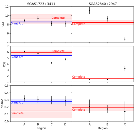
Figure 6.— Comparison of the R23, O32, and Ne3O2 values for spatially resolved regions (black points) and the values measured from spatially integrated spectra of either complete images (red) or the SGAS1723 giant arc (blue). There is a suggestion of spatial variation of R23 and clear variation of O32 in SGAS1723 and as well as significant variation in both R23 and O32 in SGAS2340. It is also clear from the disagreement between the spatially integrated values and some of the spatially resolved values that integrated spectra do not provide a complete picture of the physical conditions inside galaxies like these (see section 6.2).

The middle and bottom rows of Fig. 6 show the spatial variation in the diagnostics O32 and Ne302, which are primarily sensitive to ionization parameter. The regions in SGAS1723 show generally higher O32 than those in SGAS2340, which suggests that the ionization parameter in SGAS1723 is systematically higher than in SGAS2340. Both sources show significant spatial variation in O32. In SGAS2340, once again, region C stands out, differing from A and B at the 4$\sigma$ level, while A and B are in close agreement with each other. In SGAS1723, regions A and B show significantly higher O32 values than regions C and D (at the 5–10$\sigma$ level depending on the pair of regions); regions A and B agree with each other within 1.5$\sigma$ while there is 2.5$\sigma$ difference between C and D.

To summarize, within SGAS1723, regions A and B have higher O32 values than regions C and D; the same pattern is seen (at lower significance) for the Balmer decrement and R23. Within SGAS2340, region C displays higher O32, lower R23, and less reddening than the rest of the source.

As for Ne3O2, the values are slightly higher in SGAS1723 than in SGAS2340. We find no evidence of spatial variation of Ne3O2 in either galaxy. Because of the relatively faint [Ne III] line involved and its potential blends with nearby lines, the fractional uncertainties in Ne3O2 are relatively large (up to 25% in SGAS1723 and larger for SGAS2340), and greatly exceed any apparent variation in the observed Ne3O2 values.

5.7.3 Star Formation Rate

So far, the values that we have considered are all magnification independent because they rely only on relative fluxes, and gravitational lensing is achromatic. We can also look for variation in the H$\alpha$ flux, which is a well-known indicator of star formation (Kennicutt, 1998). Unlike the previous values discussed in this paper, though, this quantity is dependent on the magnification of each region. Table 4 shows the magnifications of each region determined using the lens models discussed in section 5.1.

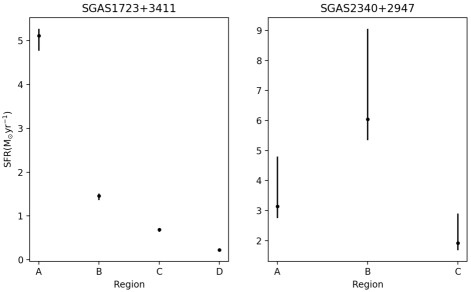
Figure 7.— Variation in star formation rate from region to region within SGAS1723 (left) and SGAS2340 (right). Both show evidence of gradients. SGAS2340 shows a negative radial gradient, with regions A and C forming stars less rapidly than region B. The SFR of SGAS1723 is driven primarily by clump A.

For each region in each source, we applied the conversion from H$\alpha$ to SFR from Kennicutt (1998) using the spatially-resolved reddening corrections and magnification corrections. There is significant spatial variation in the star formation rates across the two galaxies, as shown in Fig. 7. SGAS2340 is forming stars quite rapidly. The central region (B), exhibits the most star formation, about $6.0_{-0.7}^{+3.0}M_{\odot}yr^{-1}$, while the regions near the edges of the source (A and C) are forming about $3.1_{-0.4}^{+1.7}M_{\odot}yr^{-1}$ and $1.9_{-0.2}^{+1.0}M_{\odot}yr^{-1}$ of stars respectively. This suggests a negative radial gradient in star formation rates, but also suggests asymmetric star formation. As a check of consistency, the SFR determined by stacking all 4 complete images is $13.2_{-1.7}^{+7.1}$ M_⊙$yr^{-1}$, which agrees with the sum of the 3 subregions. Significant uncertainties remain, however, due to the lack of extra constraints for the lens model.

SGAS1723 is also undergoing rapid star formation driven by two of the three apparent clumps. Regions A and B are forming $5.11_{-0.34}^{+0.16}M_{\odot}$ and $1.46_{-0.1}^{+0.05}M_{\odot}$ per year, respectively, while regions C and D are forming stars at much lower rates, ($0.69_{-0.05}^{+0.02}M_{\odot}yr^{-1}$ and $0.23_{-0.01}^{+0.01}M_{\odot}yr^{-1}$). The northern complete image of SGAS1723 (image 3) appears to have a SFR of $7.91_{-0.39}^{+0.41}M_{\odot}yr^{-1}$, similar to the sum of these regions, suggesting that the portion of the galaxy visible in the arc accounts for nearly all of the star formation in SGAS1723. The low surface brightness diffuse light at the outskirts of SGAS1723  then, likely contains relatively little star formation (about 0.4 M_⊙yr^-1). Since the bright clumps are concentrated near the center of this galaxy, SGAS1723 may also have a negative gradient in the star formation rate. However, it is clear that the star formation is patchy and asymmetric, dominated by only two clumps.

As a check of consistency, the SFR derived from fitting the integrated spectrum of the entire giant arc (i.e., summing the spectrum of the whole arc and fitting the lines) is $6.68_{-0.20}^{+0.44}M_{\odot}yr^{-1}$, slightly lower than what we measure by summing the measured line fluxes of the individual regions (i.e., extracting spectra for each region and fitting the lines in each), but in agreement within about 1$\sigma$.

Although SGAS1723 shows evidence of patchy star formation dominated by two clumps, those clumps are centrally-located relative to the faint whisps of light evident at the ends of the arc and in image 3 that extend much further out from the center of the galaxy. Both sources, therefore, exhibit centrally-concentrated star formation. Such excesses have been interpreted as “inside-out star formation” in other work (e.g., Nelson et al., 2016 at similar redshifts, and Ellison et al., 2018 at lower redshifts).

5.8. Ionization Parameters and Metallicities

In § 5.7.2 we showed that the observable line ratios O32 and R23 vary in a statistically significant way. We now consider whether this can robustly be attributed to real differences in physical parameters. To address this question, we must convert between the observables and physical parameters by referring to photoionization models, in this case MAPPINGS v5.1 models (described in the following subsection) to infer the physical parameters logU (ionization parameter) and Z (metallicity).

5.8.1 MAPPINGS Photoizonization Model Grids

We use calibrations from Kewley et al. (2019a), and Kewley et al. (2019b) (henceforth K19a and K19b, respectively) and Nicholls et al. (2020), which are based on the latest version of results from the MAPPINGS v5.1 photoionization code (see Sutherland & Dopita, 1993; Dopita et al., 2013). MAPPINGS v5.1 includes the local Milky Way region elemental abundances for 30 elements. Nebular elemental abundances for sub-solar metallicites are scaled according to Nicholls et al. (2017). For depletion of nebular elements on to dust grains, the K19a,b models adopt the parametric models of Jenkins (2009) with a Fe depletion value of -1.5 dex. K19a,b use the atomic data for the 30 elements from the CHIANTI 8 database (Del Zanna et al., 2015). The MAPPINGS photoionization code self-consistently computes the ionization structure of the nebulae, accounting for dust absorption, radiation pressure, grain charging, and photoelectric heating of small grains (Groves et al., 2004).

The ionization parameter is the ratio of the local Lyman photon flux (cm^-2s^-1) to the local hydrogen density (cm^-3). This ionization parameter ($q$), with units of velocity, can be related to a dimension-less ionization parameter ($U$), which we use in this paper, via the speed of light: $U=q/c$. MAPPINGS defines the ionization parameter at the inner edge of the nebula. The photoionization, excitation and recombination is calculated in a detailed, self-consistent manner in linear increments of 0.02 step size through the nebula. See López-Sánchez et al. (2012) for a full description of the models and geometries.

The K19a,b calibrations use constant pressure models with plane parallel geometry. The ISM pressure values range from $\log{(P/k)}=4.0$ to $\log{(P/k)}=9.0$ in increments of 0.5 dex. This pressure corresponds to the total mechanical energy flux imparted on the nebula by the driving stellar source, through contributions from both stellar winds and supernovae. These models compute a detailed temperate and density structure throughout the nebulae, dictated by the metallicity and ionization structure.

For the purpose of calibrating electron density diagnostics, K19a use constant density models with electron densities ranging from $\log{(n_{e}/cm^{3})}$ = 0 to $\log{(n_{e}/cm^{3})}=5$ in increments of 0.5 dex. These models compute a temperature structure in the nebula, but unlike the isobaric models do not allow for a density structure. K19a point out that the isobaric models are the most realistic given that the sound crossing timescale in typical nebulae is shorter than the cooling/heating timescale which allows for the pressure to equalize throughout the nebula.

The metallicity ($12+\log{\mathrm{O/H}}$) values in the models are constrained by the stellar tracks, which use a coarse grid of $12+\log{\mathrm{O/H}}$ = 7.63, 8.23, 8.53, 8.93 and 9.23. The models are computed for a range of ionization parameter values from $\log{(q)}=6.5$ to $\log{(q)}=8.5$, in increments of 0.25 dex. This range corresponds to $\log{(U)}\simeq-4$ to $\log{(U)}\simeq-2$, which covers the typically observed values in H II regions (Dopita et al., 2000).

5.8.2 Variation in ionization parameter and metallicity based on MAPPINGS models

The grids used in this section are derived from models where the pressure, $\log(P/k)$, is 6.0 for SGAS1723 and 6.5 for SGAS2340, as determined by the [O II]3727/3729 ratio measured from the ESI spectra of the giant arc (consisting of two nearly complete images) in SGAS1723 and the sum of the integrated spectra of the complete images of SGAS2340.

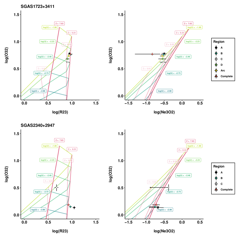
Figure 8.— Spatial variation in physical conditions logU and Z (12 + logO/H) as determined by the O32-R23 and O32-Ne3O2 planes and MAPPINGS models. Red lines indicate curves of constant metallicity, with the color saturation scaling with metallicity. Other colors correspond to curves of constant ionization parameter. Note that the MAPPINGS grid in the O32-R23 plane is double-valued and therefore folds over on itself. Spatial variation in these sources appears to be primarily driven by ionization parameter (and the O32 observable). However, the R23 values of SGAS2340also indicate significant variation in metallicity.

In Fig. 8, we plot the observed strong line ratios for each region in SGAS1723 and SGAS2340, as well as for the northern complete image and the giant arc in SGAS1723 and the stacked spectra of the complete images of SGAS2340 (three images from one roll, and one image from the other as summarized in Table 2) in the O32–R23 and O32–Ne3O2 planes. These points are overlaid on the MAPPINGS grids, from which we infer ionization parameter ($\log U=\log q/c$) and metallicity ($Z=12+\log(O/H)$). Characteristically, the grids in the O32–R23 plane are double-valued; most of our points fall near the double-valued region or where the grids fold over. Consequently, the interpretation of these inferred parameters will have some amount of degeneracy in that there is both a high-metallicity interpretation and a low-metallicity interpretation. The [N II]/H$\alpha$ flux ratio from GNIRS, approximately 6.2% for region A of SGAS1723 and 8.4% region B of SGAS2340, suggest that these regions do fall almost exactly on the fold. The MAPPINGS models suggest a metallicity near $12+\log(O/H)\sim 8.23$ for both sources, though it could be as high as 8.6 for SGAS1723 if it is on the higher metallicity branch. Similarly, the first-order formula of Pettini & Pagel (2004) returns a metallicity of $8.21\pm 0.04$ for SGAS1723 and $8.29\pm 0.09$ for SGAS2340. Their third-order formula returns $8.19\pm 0.03$ for SGAS1723 and $8.25\pm 0.07$ for SGAS2340. Additionally, the ratio of [O II] 2470Å to [O III] 3727/3729Å can be used as a temperature diagnostic, which predicts a temperature of 11,384${}^{+3067}_{-2759}$K for SGAS2340(similar to, but slightly higher than the what Rigby et al., in prep, finds for SGAS1723 ), and also suggests a moderate metallicity (Nicholls et al., 2020).

For SGAS1723, we see that most of the variation is in O32, not in R23. The model grids indicate that this largely corresponds to variation in the ionization parameter. Regardless of which metallicity branch is assumed, the $\log U$ in each region is between $-2.23$ and $-2.48$, for a spread of a little less than 0.25 dex in ionization parameter. If the points are on the low-metallicity branch, then they fall near, but slightly below $Z=8.23$ with very little spread. However, if they are on the high metallicity branch, they fill the region $Z=8.23$ to $Z=8.53$, with a spread of about 0.30 dex.

The O32–Ne3O2 plane suggests that SGAS1723 has a slightly higher ionization parameter than the O32–R23 plane implies, with values falling between $\log U=-1.98$ and $\log U=-2.23$; the spread is similar, still about 0.25 dex. Again, the variation is almost entirely in the ionization parameter and is most apparent in the O32 dimension. Unlike the O32–R23 grid, the Ne3O2–R23 grid is not double-valued, and the Ne3O2 values suggest that the metallicity in every region of SGAS1723 is somewhat higher than we inferred from the O32–R23 grids. Still, if we assume that this means that SGAS1723 falls on the high-metallicity branch in O32–R23 space, then those metallicities agree with the Ne302–R23 metallicities.

SGAS2340 is quite different from SGAS1723 in a number of ways. Of particular interest is the more extreme spatial variation. While regions A and B are very similar in both ionization and metallicity, region C is nothing like them. Both grids, O32 vs R23 and O32 vs Ne3O2, show that regions A and B, as well as the complete image, have ionization parameters that are tightly bunched about halfway between $\log U=-2.73$ and $\log U=-2.98$ (i.e., around $\log U=-2.85$). This is not the case for region C, which has a much higher ionization parameter. While the lack of a robust detection in Ne3O2 diminishes its utility as an indicator of ionization parameter, the location of region C in the O32–R23 plane suggests that it has an ionization parameter of either $\log U\sim-2.65$ (low metallicity branch) or $-2.23$ (high metallicity branch). In the low metallicity case, the offset between region C and the other regions in ionization parameter is about the same size as the spread in ionization parameters across the different regions of SGAS1723. In the high metallicity case, the offset may be more than twice as large. Unlike SGAS1723, though, this variation is driven by a single unique region—the rest of SGAS2340 is nearly uniform in $\log U$.

The interpretation of metallicity for SGAS2340 is a little more difficult because some of the points, particularly in the O32–R23 plane fall outside the model grid. This is likely a real phenomenon, as these points lie in a region of the O32–R32 plane that is populated by z$\sim$2 galaxies in MOSDEF (Reddy et al., 2018), z$\sim$2–3 galaxies in Nakajima et al. (2013), and z$\sim$3.3 galaxies in Onodera et al. (2016). Why the models do not account for this is unclear, but there are several sources of uncertainty in the photoionization models that could lead to this. Nonuniform conditions within emission regions, uncertainties in the calibrations of strong line diagnostics, and uncertainties in atomic data all contribute to uncertainties in the location of grid points. If we assume that the points that fall off of the O32–R23 grids for SGAS2340 are actually at or near the grid’s fold, then the metallicity is around $Z=8.23$.

Small uncertainties in the Ne3O2 ratio correspond to large uncertainties in the inferred $Z$ from the O32–Ne3O2 grid. Still, that grid indicates that regions A and B and the complete image fall at relatively low $Z$, around $7.63$ to $8.23$; however, it does not rule out metallicities as high as $8.53$. Region C, based on O32 vs R23, can either be around $Z\sim 7.7$ if on the low metallicity branch, or $\sim 8.8$ if on the high metallicity branch. Since region C has a higher ionization parameter than the other regions and is substantially less reddened, it would seem reasonable for it to be on the low metallicity branch. However, we do not have a [N II]/H$\alpha$ measurement for this region to break the degeneracy.

Overall, these two galaxies exhibit variation in ionization parameter of at least $0.25$ dex. The metallicity variation is probably smaller, but the double-valued O32–R23 grid makes it difficult to say definitively. The variations in ionization and metallicity in SGAS1723 manifest as slight variation across the different regions. Regions A and B are more similar to each other in all of $\log U$, $Z$, $E(B-V)$, and SFR, than they are to regions C or D (which themselves are more like each other than they are like A or B). Because of the proximity of A to B and C to D, this looks like the physical conditions are, perhaps, spatially correlated, but they are not necessarily representative of a radial gradient (since the morphology is so clumpy and the variations are driven by differences in the clumps) and may simply be indicative of asymmetry. It is much clearer, though, that the variation in SGAS2340 is driven almost entirely by one single spatial region (C) that is very different from the others, especially in $\log U$, $Z$, $E(B-V)$. This, too, appears more like an asymmetry than a radial gradient except in SFR. It is possible that these asymmetries are indicative of a recent or ongoing merger (e.g., region C being accreted by a galaxy composed of regions A and B).

6. Discussion

In the previous sections, we presented observational evidence for significant spatial variation in strong line ratios and the physical conditions that drive them across two galaxies at $z\sim 1.4$. This finding has significant implications for interpreting current observations of field galaxies, as well as implications for planning future observations; here, we explore some of these potential impacts. We focus primarily on observable strong line ratios, rather than physical parameters like $U$ and $Z$, because direct observables are model-independent.

6.1. Reddening

The finding that reddening can vary spatially across $z\sim 1.4$ galaxies should not be surprising, but it importantly affects the interpretation of other observed strong line ratios. Fig. 5 shows the H$\alpha$/H$\beta$ ratios for each spatially-resolved region, compared to the ratios from the spatially-integrated spectra. While there may be slight tension between the value for region B in SGAS1723 and the value derived from the spectrum of the whole arc, there is relatively little variation in reddening throughout the regions visible in the giant arc, and no conflict with the line ratio measured from the spectrum of the complete image, despite the fact that it contains more of the underlying source galaxy than just the regions contained in the arc. This is not particularly surprising, though, since the part of the source that is not imaged in the arc is relatively small, with low surface brightness compared to the rest of the source. It is actually somewhat remarkable that the reddening in the individual regions agrees so well with the reddening of the arc and the complete image despite the spectra of the latter two being essentially wavelength-by-wavelength flux-weighted averages of the spectral properties of regions A–D. This did not have to be the case, as shown clearly by the H$\alpha$/H$\beta$ ratios in SGAS2340. The line ratio in the spectra of the complete images is much more representative of the bright, similarly-reddened regions A and B than it is of the much fainter and much less reddened region C.

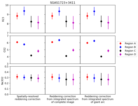
Figure 9.— From top to bottom, R23, O32 and Ne3O2 of individual spatially-resolved regions in SGAS1723 color-coded by region. Each column of plots displays these values determined using different reddening corrections. Using a reddening correction derived from the spatially-resolved spectra(left column) clearly influences the O32 value of region B and brings it below the value of region A, compared to using reddening corrections from the spectrum of the complete image (middle column), or the spectrum of the entire giant arc (right column). This demonstrates the potential importance of obtaining spatially-resolved reddening indicators rather than assuming a single uniform reddening for an entire galaxy.

With this in mind we explore the consequences of using spatially-integrated reddening corrections to spatially-resolved spectra, as one might want to do for higher redshift targets where the H$\alpha$ line is shifted redward of the G141 grism. Figs. 9 and 10 show the difference between the measured values of R23, O32 and Ne3O2 with a spatially-resolved reddening correction applied compared to what we would get using a global correction from either the complete images of SGAS1723 or SGAS2340, or the giant arc for SGAS1723. Fig. 9 shows the impact on the reddening-corrected R23, O32, and Ne3O2 ratios. While individual values do not typically change by much, the slight excess in reddening observed in region B is enough to have an important effect on its O32 ratio. By not using spatially-resolved values of H$\alpha$/H$\beta$, we would incorrectly infer that the value of O32 in region B is actually higher than in region A, even though this is not the case. While the overall change is low, this type of uncertainty could influence searches for spatial gradients in ionization parameter or metallicity. In SGAS2340 (Fig. 10), we see no such changes in ordering, but the value of O32 in region C is noticeably underestimated. Since high O32 correlates with leakage of ionizing photons, searches for LyC leakers that depend on indirect indicators like O32 could miss candidates if they apply spatially integrated reddening corrections.

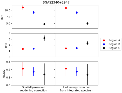
Figure 10.— The same as Fig. 9 except for SGAS2340. In this case there is no giant arc, so the left column uses spatially-resolved H$\alpha$ to H$\beta$ ratios to de-redden the spectra, while the right column uses the ratio from the stack of the complete images. Once again this has a noticeable impact on O32. In particular, O32 is higher in region C when spatially-resolved reddening corrections are used. This is likely because its reddening is much lower than that what would be inferred from the spectrum of the complete image as shown in Fig. 5.

The fact that spatially-resolved reddening corrections can have this kind of impact is a particularly important consideration for planning observations in the near-term because there is only a small window of redshifts where the [O II] 3727/3729 doublet and the H$\alpha$ line are both observable with space-based, spatially-resolved spectroscopy at this point in time (z$\sim$1.15–1.58 with the HST WFC3/IR grisms). Without both of these features one cannot determine a reddening-corrected value of the O32 diagnostic, for instance.

These two objects were chosen to fall within that window, but most potentially interesting targets will not. It may be tempting to extend this window by assuming spatially uniform reddening and using a spatially-integrated H$\alpha$ measurement from ground-based spectroscopy, for example, to determine the reddening. Doing so would expand the observable redshift range to $z\sim 2.4$ by making the reddest line of interest the [O III] 5007 doublet instead of H$\alpha$. While this may work for sources like SGAS1723 where the reddening is relatively uniform spatially, it could cause problems for sources like SGAS2340 where there is significant variation in reddening. In fact, as we have seen here, even the relatively low variation in reddening within SGAS1723 may be enough to meaningfully affect the interpretation of strong line ratios of a region like B.

When reddening cannot be measured in a spatially resolved way, it is likely that regions of higher extinction will be missing or under-represented. This presumably also affects HST surveys that use broad-band rest-frame UV light as a tracer of star formation as well as H$\alpha$–based surveys with the HST grisms. Real progress will come with spectroscopy from the IFUs on JWST’s NIRSPec and MIRI instruments, which will be able to measure spatially-resolved H$\alpha$/H$\beta$ ratios—and better yet, Paschen $\alpha$ / H$\alpha$ ratios—over a much larger range of redshift than is possible with the HST WFC3-IR grisms. Until then, interpretation of spatially-resolved spectroscopic studies of galaxies with redshifts above 1.58 with the HST grisms will suffer from serious uncertainties due to the unconstrained reddening variation.

6.2. O32, R23, Ne3O2

We do not detect statistically significant spatial variation in Ne3O2. This is at least partly due to the fact that [Ne III] 3869 is difficult to disentangle from nearby lines at the low spectral resolution of the HST grisms. In addition, in the MAPPINGS models, while Ne3O2 is more sensitive to $Z$ than to $\log U$, small uncertainties in Ne3O2 can translate to large uncertainties in $Z$, such that it does not usefully constrain $Z$. R23, which does show significant spatial variation, more powerfully discriminates between different Z values than does Ne3O2. The downside is that the MAPPINGS grid is double-valued in the O32–R23 plane, and the spectrographs with high spatial resolution at these wavelengths (WFC3-IR grisms) lack the spectral resolution to obtain other spatially–resolved indicators to break the degeneracy. Ultimately, high spectral resolution, high spatial resolution spectroscopy of lensed galaxies is necessary to break the degeneracy by obtaining, for instance, a spatially-resolved [N II]/H$\alpha$ ratio. This will be firmly within the capabilities of JWST  IFU spectroscopy, for instance (and indeed, SGAS1723 will be observed as part of the JWST Early Release Science program, TEMPLATES; PI: Rigby).

We confidently detect spatial variation in the O32 and R23 ratios. By necessity, most of the spectroscopy of distant ($z\gtrsim 1$) galaxies is spatially integrated, so we now compare the spatially-integrated values of O32, R23 and Ne3O2 to the spatially-resolved values to see what, if anything, we are missing in typical observations. Fig. 6 shows this comparison. There are clear differences in the results. The value of R23 measured from the complete image of SGAS2340 is most in agreement with the value for region B. However, the values for regions A and C lie significantly higher and lower, respectively, than the value for the complete image. Meanwhile, even though the O32 value for the SGAS2340 complete images is near the values for regions A and B, it is significantly below the value for region C.

SGAS1723 further illustrates how spatially integrated spectra can obscure the actual physical conditions within a galaxy. While the O32 value for the complete image agrees with the values in regions A and B, it disagrees with the values for regions C and D, and is only barely compatible with the value for the integrated spectrum of the entire giant arc. The value for the giant arc, interestingly, lies below the values for regions A and B, but above the values for regions C and D. Even though there is general agreement between the spatially-resolved and the spatially-integrated values of R23, it is clear that, in general, the physical conditions in subregions are not necessarily well represented by the values inferred from spatially integrated spectra of either complete images or giant arcs. Just as studies of the stacked spectra of many galaxies miss the unique characteristics of individual galaxies, so too do the integrated spectra of single galaxies miss the unique characteristics of individual physical regions within them.

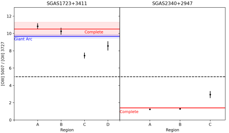
Figure 11.— A slightly different parameterization of the [O III] to [O II] ratio, this time [O III] 5007 / [O II] 3727. This ratio has been suggested to be an indicator of possible LyC leakage if it exceeds 5 (dashed line). Since the spatially-resolved grism spectra cannot spectrally resolve the 3727/3729 doublet, the value of that ratio is set based on the ground-based spatially-integrated ESI spectra (though based on the Figs. 5 and  6, it is not necessarily good to assume that ratios like this do not vary spatially). While the spatially resolved spectra do not result in identifications of LyC leakers where the spatially integrated spectra did not for these two specific sources, SGAS2340 in particular suggests that this may not always be the case.

6.3. Implications for finding galaxies that leak ionizing photons

Galaxies with high O32 ratios are found to be leaking ionizing photons at much higher rates than the general galaxy population (e.g.  Izotov et al. 2018; Nakajima et al. 2013). In particular, Izotov et al. (2018) suggests that a flux ratio of [O III] 5007 / [O II] 3727 $\gtrsim 5$ is necessary but not sufficient for a galaxy to be leaking ionizing photons. (Note: While this is a ratio of [O III] to [O II], it is not the same definition that we have been using for O32 in this paper. See discussion in §5.7.2.) In Fig. 11, we plot this ratio (using their definition) for each of the regions in SGAS1723 and SGAS2340 as well as for the spatially-integrated spectra to determine how using spatially-integrated spectra would have influenced a search for LyC leakers that included SGAS1723 and SGAS2340. The [O II] 3727 and 3729 lines are not resolved in the grism spectra, so in order to assign a value of [OII ] 3727 to each region, the blended [O II] 3727 + 3729 values were multiplied by the spatially-integrated 3727/3729 ratio determined from the ground-based ESI data. For SGAS1723, this is the value for the integrated spectrum of the giant arc. For SGAS2340, this is the value for the summed integrated spectra of all four complete images.

In neither case would the complete or giant arc values have suggested that the source was not a leaker when small regions inside it were leaking. For SGAS1723, all four regions lie well above the threshold of 5. The giant arc and complete image also yield large values. However, the values for regions C and D are somewhat lower than for regions A and B, and they drag down the value measured for the giant arc. So while SGAS1723 would likely have remained on any list of LyC candidates based on this criterion alone, it may have been given a lower priority for follow-up than it deserves, since region A is a stronger candidate for leakage than the spectrum of the sum of the giant arc would suggest.

SGAS2340, while having no region that exceeds [O III] 5007 / [O II] 3727 $=$ 5, still suggests that it is quite possible to miss a candidate by looking only at spatially-unresolved spectra. The value for region C is much higher than what is implied by the complete image. And while it is still well below 5, it is not hard to imagine a similar case where the points are all shifted slightly upward and the complete image shows low [O III] 5007 / [O II] 3727, but one small spatial region, like region C, lies above the threshold. If the physical processes that lead to the conditions that enable the escape of ionizing photons are spatially isolated events rather than large galaxy-wide phenomena, then surveys using spatially-integrated spectra can be expected to systematically miss candidates with only one or a few leaking regions. In fact, it is already known that at least some objects exist where LyC leakage is a local, rather than galaxy-scale event (e.g., Rivera-Thorsen et al., 2019), so this concern must be taken seriously as a potential source of bias.

7. Conclusions

To summarize, using spatially-resolved grism spectroscopy of two highly magnified star-forming galaxies at $z=1.33$ and $z=1.42$, we have explored the extent of spatial variation in observable strong diagnostic lines and the model-dependent physical parameters that they imply. We have also examined potential implications of such variation for interpreting existing data and for planning future observations, including with the JWST IFUs. The following bullet points summarize our main findings.

• There is statistically significant variation in strong-line ratios like O32 and R23, but any variation in the Ne3O2 diagnostic is below the level that we can measure in this type of data.

• These variations lead to spreads of about 0.2-0.5 dex in metallicity and ionization parameter, depending on which metallicity branch these regions reside on in the R23–O32 plane.

• The Balmer decrement, H$\alpha$/H$\beta$ varies significantly within a single source galaxy. Spatially-integrated spectra yield values of this ratio (and of R23 and O32) that may differ substantially from that of individual, distinct physical regions within a single galaxy. Furthermore, applying spatially-integrated reddening corrections to spatially-resolved line fluxes can improperly influence the inferred values of other diagnostic ratios like R23 and O32.

• The star formation in these sources is concentrated near the center of these galaxies, suggesting that they are perhaps undergoing inside-out star formation. Each source also displays a rather large degree of asymmetry in star-formation rates. For SGAS1723 this is apparent even among the bright, star-forming clumps concentrated near the center of the source. The morphology of its star formation is perhaps more characterized by its clumpiness than a radial gradient. It is worth considering whether calculating azimuthally-averaged gradients in properties like SFR is still an effective metric when applied to high-resolution data since asymmetries in annuli would make such a measurement quite misleading in a source like SGAS1723. Curti et al. (2020) raise the same issue in the context of metallicity maps. Perhaps, in high spatial-resolution data, a metric like the clumpiness indices or Gini coefficients of properties like SFR, metallicity, etc. could be more informative.

• If O32 is used as an indirect indicator of possible LyC leakage, then sources in which only a single or a few small regions are leaking LyC photons may systematically be undercounted in surveys that use spatially integrated spectra. Extreme O32 ratios in a single region, for example, can be drowned out by less extreme ratios in the rest of the source, causing a more moderate O32 value to be measured from the integrated spectrum.

• SGAS1723, based on the O32 values in each of its spatial regions, is a candidate for LyC leakage. SGAS2340 has less extreme ratios and is not as good of a candidate.

Appendix A Stellar mass estimates

Total stellar masses for each of these objects were determined using the MCMC-based stellar population synthesis and parameter inference code, Prospector (that is based on the python-FSPS framework, with the MILES stellar spectral library and the MIST set of isochrones; Conroy & Gunn, 2010; Foreman-Mackey et al., 2013; Johnson & Leja, 2017; Leja et al., 2017).

As input to this code, we used the demagnified magnitudes of each of these objects from the avaiable HST and Spitzer bands. For SDSS J1723$+$3411, we used the magnitudes of the giant arc, which required us to apply a correction to account for the fact that it is a merging set of two nearly (but not totally) complete images. For SDSS J2340$+$2947the photometry was summed across the three most magnified images, ignoring the less magnified counterimage (image 4) that is closer to the BCG and more contaminated by light from cluster galaxies. For each source, fluxes were corrected for Milky Way reddening.

We created detailed models for the light profiles of each of these objects using GALFIT (Peng et al., 2002) and calculated the photometry from these models. For the HST images, the models describe the lensed galaxies and the BCG, as well as any other cluster members or nearby foreground or background galaxies that may contaminate the light profiles of the lensed sources. Point spread functions (PSFs) were derived from the data directly, by summing appropriately isolated point source images surrounding the model region. The initial model was constructed using a sum of the F390W and F814W (or F775W) images. This initial model was then propagated to individual HST filter images by re-optimizing it, allowing for small ($\sim 20\%$) variations in fitted structural parameters in each step in wavelength away from the initial model, in addition to freely varying the magnitudes of the model components. Examples of these models are shown in Fig. 12 Total magnitudes of each lensed source were then derived by summing the flux across all relevant structural components that comprise each image. Simple aperture photometry - derived from HST images with the fitted central lens galaxy image removed, is consistent with these more complex measurements.

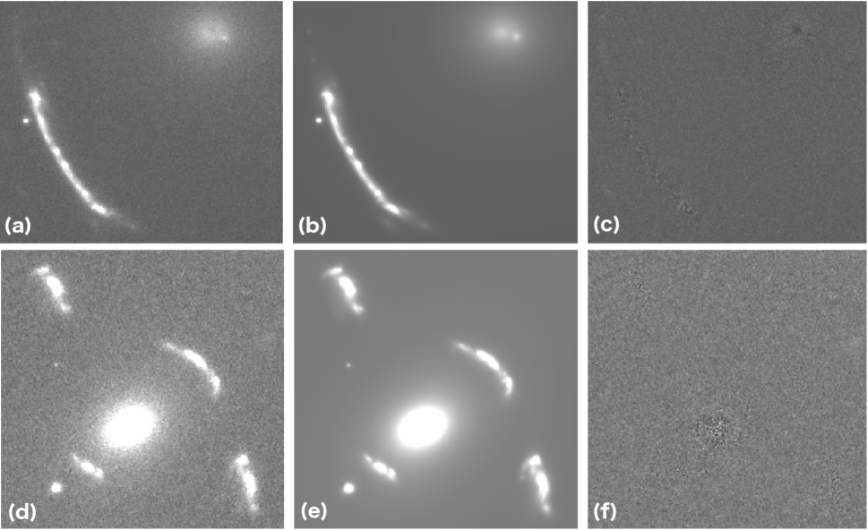
Figure 12.— Direct images, GALFIT models, and residuals for SGAS1723 and SGAS2340. (a): The stack of the F390W and F775W images of SGAS1723. (b): The GALFIT model of (a). (c): The difference (residual) of (a) and (b). (d): The F814W image of SGAS2340. (e): The GALFIT model of (d). (f): The difference (residual) of (d) and (e).

The Spitzer PSF has broad enough wings that this it was necessary to include additional model components to describe other nearby objects to enable a robust sky measurement in the modeling. The HST-derived model of the lensed sources is, in practice, more complex than necessary to describe them in the Spitzer data. In fits in which the source components are essentially unconstrained, it is thus typical that some components trend toward zero flux. Experiment shows that constrained fits, in which the components are all required to be significant, produce the same measurement in that the total flux summed across all the components that describe a given lensed image of the source is consistent.

Demagnified and Milky Way reddening-corrected magnitudes are tabulated for the SGAS1723 and SGAS2340 in Table 6. These magnitudes serve as constraints for the stellar population modeling. In these models for SGAS2340  we assumed a parametric star formation history (simple tau model, with e-folding time $\tau$ and star formation start time $sf_{start}$, both in Gyr), dust attenuation applied to all light from the galaxy (in units of opacity at 5500Å), metallicity $log(Z/Z_{\odot})$ (where $Z_{\odot}=0.0142$), and total mass formed in the galaxy (in M_⊙), as free parameters. The dust extinction and metallicity have priors covering the 2$\sigma$ range suggested by the available spectroscopy. For SGAS1723  which was consistent with zero reddening, we used a dust-free model. These models each assumed a Kroupa IMF (Kroupa 2001) and that nebular continuum and line emission are present. We assumed the WMAP9 cosmology (Hinshaw et al., 2013) where necessary.

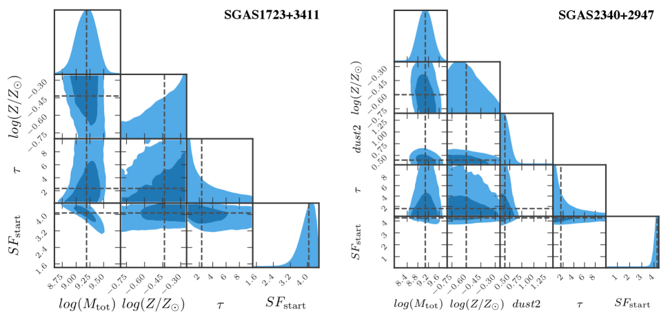
Figure 13.— Corner plots for the SED models of SGAS1723 (left) and SGAS2340 (right). M_tot is the stellar mass in units of solar masses. Z/Z_⊙ is the metallicity relative to solar metallicity. $\tau$ is the star formation e-folding time in Gyr. SF_start is the time, in Gyr, at which star formation began. SGAS1723 was modeled as if it were dust-free (consistent with the Balmer decrement), while our model for SGAS2340 included fitting for dust within a range determined by the measured Balmer decrement and its uncertainties. The parameter, dust2, is the optical depth of the dust at 5500Å .

As seen in the corner plots (Fig. 13), the total mass parameter converges to a tailed Gaussian posterior distribution for these sources, which corresponds to model-generated remnant stellar mass distributions (Figure 14). The favored model for each of these sources is a recent burst of star formation, corroborated by strong emission features—Ly$\alpha$, H$\alpha$, H$\beta$, H$\gamma$ H$\delta$, OIII[5007]—throughout the best fit model spectra (Fig. 15 and Fig. 16 for SGAS1723 and SGAS2340 respectively).

For SGAS2340  the remnant stellar mass, based on stellar population synthesis (SPS) fitting to the 6 photometric data points from HST and Spitzer, is $9.6^{+0.7}_{-0.4}\times 10^{8}$ M_⊙. The uncertainties used in the SPS fitting do not include the system-wide magnification uncertainty, which when combined with the statistical uncertainties, yields a final mass of $9.7^{+9.0}_{-4.4}\times 10^{8}$ M_⊙. We should note, however, that the models preferred a dust value slightly outside of the $2\sigma$ constraint inferred from the Balmer decrement. Relaxing this constraint resulted in the model running to a slightly lower value of the dust2 parameter, but still yielding a stellar mass that agrees within $1\sigma$ ($1.5^{+1.1}_{-0.7}\times 10^{9}$ M_⊙).

For SGAS1723, the remnant stellar mass, based on 8 photometric data points from HST and Spitzer for the giant arc, is $1.190^{+0.440}_{-0.371}\times 10^{9}$ M_⊙. Because of the excellent constraints on the lens model of SGAS1723  the uncertainties are dominated by statistical uncertainties in the SED fitting rather than by the magnification uncertainties. The arc, however, includes two nearly complete images of the source, so this value must be adjusted by about a factor of two. Figure 17, shows the location of the caustic in the source reconstruction of images 1 through 4. Image 3 is a complete image and the exact location of the caustic is better determined for it than for image 4, so we use image 3 to estimate the fraction of the source that is visible in the arc. To do this, we first drew a custom aperture around the source reconstruction of the stacked UVIS images of image 3. The UVIS data was chosen because the higher spatial resolution means less flux will be spread across the critical curve by the wings of the PSF. We then modified that aperture so that it did not cross the caustic (i.e., so that it contained only the portion of the galaxy imaged in the arc). 95.7% of the flux contained in the original aperture is contained in the modified aperture, so the two images of the source galaxy that make up the giant arc are each about 95.7% complete. We therefore adjust the stellar mass estimate by $2\times 0.957$, or a factor of 1.914. This results in a stellar mass estimate of $5.95^{+2.2}_{-1.86}\times 10^{8}$ M_⊙ for SGAS1723.

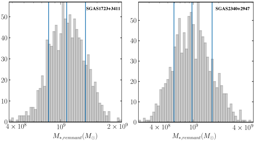
Figure 14.— Posterior distribution for the observed remnant stellar masses, constructed from SPS models corresponding to 10000 random chains for SGAS1723 (top) and SGAS2340 (bottom). Vertical lines, from left to right, denote the $16^{th}$, $50^{th}$, and $84^{th}$ percentiles.

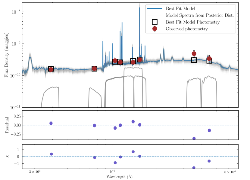
Figure 15.— Top panel: The best fit spectrum for SGAS1723 is plotted here in blue. To visualize the spread in model predictions, 1000 other high-likelihood model spectra are plotted in gray. Photometry from HST and Spitzer data are plotted as red ciricles, with black error bars, while the photometry predicted by the best fit model is plotted as black squares. For reference, the shapes of the transmission curves for the six HST filters and two Spitzer channels are plotted at the bottom. Middle: The residual (model minus observed photometry). Bottom: The $\chi$-value (residual divided by uncertainty) for each point.

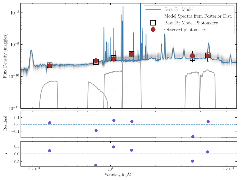
Figure 16.— The observed photometry, best fit model spectrum, distribution of model spectra, residuals, and $\chi$-values for SGAS2340. Colors and labels follow the same pattern as Fig. 15

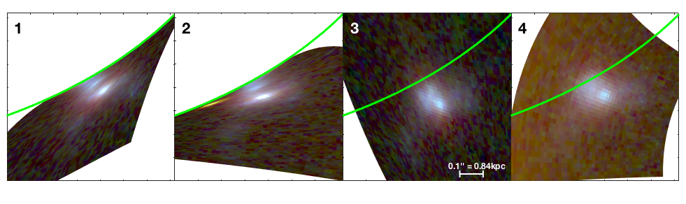
Figure 17.— Source reconstructions of four of the five images of SGAS1723 labeled as they appear in Fig. 1. Caustics are plotted in green. We used image 3 to compute the fraction of the source visible in images 1 and 2 in order to correct the stellar mass calculation.

Source	Band	Magnitude	Uncertainty*
SGAS1723	IRAC Ch1	23.28	0.25
	IRAC Ch2	23.66	0.25
	F160W	23.75	0.15
	F140W	23.95	0.15
	F110W	23.95	0.10
	F105W	23.82	0.10
	F775W	24.44	0.10
	F390W	24.52	0.15
SGAS2340	IRAC Ch1	23.36	0.40
	IRAC Ch2	23.39	0.34
	F140W	23.26	0.19
	F105W	23.60	0.14
	F814W	23.76	0.14
	F390W	24.15	0.12

Table 6Integrated photometry for the arc in SGAS1723 and for the complete image of SGAS2340 determined by combining the three most magnified images. All values are demagnified. *Uncertainties do not include the magnification uncertainty.

References

- Acharyya et al. (2019) Acharyya, A., Kewley, L. J., Rigby, J. R., Bayliss, M., Bian, F., Nicholls, D., Federrath, C., Kaasinen, M., Florian, M., & Blanc, G. A. 2019, MNRAS, 488, 5862
- Belfiore et al. (2017) Belfiore, F., Maiolino, R., Tremonti, C., Sánchez, S. F., Bundy, K., Bershady, M., Westfall, K., Lin, L., Drory, N., Boquien, M., Thomas, D., & Brinkmann, J. 2017, MNRAS, 469, 151
- Bertin & Arnouts (1996) Bertin, E. & Arnouts, S. 1996, A&AS, 117, 393
- Carton et al. (2018) Carton, D., Brinchmann, J., Contini, T., Epinat, B., Finley, H., Richard, J., Patrício, V., Schaye, J., Nanayakkara, T., Weilbacher, P. M., & Wisotzki, L. 2018, MNRAS, 478, 4293
- Conroy & Gunn (2010) Conroy, C. & Gunn, J. E. 2010, FSPS: Flexible Stellar Population Synthesis
- Curti et al. (2020) Curti, M., Maiolino, R., Cirasuolo, M., Mannucci, F., Williams, R. J., Auger, M., Mercurio, A., Hayden-Pawson, C., Cresci, G., Marconi, A., Belfiore, F., Cappellari, M., Cicone, C., Cullen, F., Meneghetti, M., Ota, K., Peng, Y., Pettini, M., Swinbank, M., & Troncoso, P. 2020, MNRAS, 492, 821
- Del Zanna et al. (2015) Del Zanna, G., Dere, K. P., Young, P. R., Landi, E., & Mason, H. E. 2015, arXiv, A56
- Dopita et al. (2000) Dopita, M. A., Kewley, L. J., Heisler, C. A., & Sutherland, R. S. 2000, ApJ, 542, 224
- Dopita et al. (2014) Dopita, M. A., Rich, J., Vogt, F. P. A., Kewley, L. J., Ho, I. T., Basurah, H. M., Ali, A., & Amer, M. A. 2014, Ap&SS, 350, 741
- Dopita et al. (2013) Dopita, M. A., Sutherland, R. S., Nicholls, D. C., Kewley, L. J., & Vogt, F. P. A. 2013, The Astrophysical Journal Supplement Series, 208, 10
- Elias et al. (2006) Elias, J. H., Joyce, R. R., Liang, M., Muller, G. P., Hileman, E. A., & George, J. R. 2006, Ground-based and Airborne Instrumentation for Astronomy. Edited by McLean, 6269, 62694C
- Elíasdóttir et al. (2007) Elíasdóttir, Á., Limousin, M., Richard, J., Hjorth, J., Kneib, J.-P., Natarajan, P., Pedersen, K., Jullo, E., & Paraficz, D. 2007, arXiv e-prints, arXiv:0710.5636
- Ellison et al. (2018) Ellison, S. L., Sánchez, S. F., Ibarra-Medel, H., Antonio, B., Mendel, J. T., & Barrera-Ballesteros, J. 2018, MNRAS, 474, 2039
- Elmegreen et al. (2005) Elmegreen, D. M., Elmegreen, B. G., Rubin, D. S., & Schaffer, M. A. 2005, ApJ, 631, 85
- Foreman-Mackey et al. (2013) Foreman-Mackey, D., Conley, A., Meierjurgen Farr, W., Hogg, D. W., Lang, D., Marshall, P., Price-Whelan, A., Sanders, J., & Zuntz, J. 2013, emcee: The MCMC Hammer
- Girard et al. (2018) Girard, M., Dessauges-Zavadsky, M., Schaerer, D., Richard, J., Nakajima, K., & Cava, A. 2018, A&A, 619, A15
- Gladders & Yee (2000) Gladders, M. D. & Yee, H. K. C. 2000, AJ, 120, 2148
- Green et al. (2015) Green, G. M., Schlafly, E. F., Finkbeiner, D. P., Rix, H.-W., Martin, N., Burgett, W., Draper, P. W., Flewelling, H., Hodapp, K., Kaiser, N., Kudritzki, R.-P., Magnier, E., Metcalfe, N., Price, P., Tonry, J., & Wainscoat, R. 2015, ApJ, 810, 25
- Groves et al. (2004) Groves, B. A., Dopita, M. A., & Sutherland, R. S. 2004, The Astrophysical Journal Supplement Series, 153, 9
- Guo et al. (2012) Guo, Y., Giavalisco, M., Ferguson, H. C., Cassata, P., & Koekemoer, A. M. 2012, ApJ, 757, 120
- Hinshaw et al. (2013) Hinshaw, G., Larson, D., Komatsu, E., Spergel, D. N., Bennett, C. L., Dunkley, J., Nolta, M. R., Halpern, M., Hill, R. S., Odegard, N., Page, L., Smith, K. M., Weiland, J. L., Gold, B., Jarosik, N., Kogut, A., Limon, M., Meyer, S. S., Tucker, G. S., Wollack, E., & Wright, E. L. 2013, ApJS, 208, 19
- Holden et al. (2016) Holden, B. P., Oesch, P. A., González, V. G., Illingworth, G. D., Labbé, I., Bouwens, R., Franx, M., van Dokkum, P., & Spitler, L. 2016, ApJ, 820, 73
- Izotov et al. (2018) Izotov, Y. I., Worseck, G., Schaerer, D., Guseva, N. G., Thuan, T. X., Fricke, V. A., & Orlitova, I. 2018, Monthly Notices of the Royal Astronomical Society, 478, 4851
- Jenkins (2009) Jenkins, E. B. 2009, ApJ, 700, 1299
- Johnson & Leja (2017) Johnson, B. & Leja, J. 2017, Bd-J/Prospector: Initial Release
- Johnson et al. (2017) Johnson, T. L., Sharon, K., Gladders, M. D., Rigby, J. R., Bayliss, M. B., Wuyts, E., Whitaker, K. E., Florian, M., & Murray, K. T. 2017, ApJ, 843, 78
- Jones et al. (2010) Jones, T. A., Swinbank, A. M., Ellis, R. S., Richard, J., & Stark, D. P. 2010, Monthly Notices of the Royal Astronomical Society, 404, 1247
- Jullo et al. (2007) Jullo, E., Kneib, J. P., Limousin, M., Elíasdóttir, Á., Marshall, P. J., & Verdugo, T. 2007, New Journal of Physics, 9, 447
- Kennicutt (1998) Kennicutt, R. C. 1998, Annual Review of Astronomy and Astrophysics, 36, 189
- Kewley & Dopita (2002) Kewley, L. J. & Dopita, M. A. 2002, The Astrophysical Journal Supplement Series, 142, 35
- Kewley et al. (2019a) Kewley, L. J., Nicholls, D. C., Sutherland, R., Rigby, J. R., Acharya, A., Dopita, M. A., & Bayliss, M. B. 2019a, ApJ, 880, 16
- Kewley et al. (2019b) Kewley, L. J., Nicholls, D. C., & Sutherland, R. S. 2019b, ARA&A, 57, 511
- Kewley et al. (2015) Kewley, L. J., Zahid, H. J., Geller, M. J., Dopita, M. A., Hwang, H. S., & Fabricant, D. 2015, The Astrophysical Journal Letters, 812, L20
- Kubo et al. (2010) Kubo, J. M., Allam, S. S., Drabek, E., Lin, H., Tucker, D., Buckley-Geer, E. J., Diehl, H. T., Soares-Santos, M., Hao, J., Wiesner, M., West, A., Kubik, D., Annis, J., & Frieman, J. A. 2010, ApJ, 724, L137
- Leja et al. (2017) Leja, J., Johnson, B. D., Conroy, C., van Dokkum, P. G., & Byler, N. 2017, ApJ, 837, 170
- Levesque & Richardson (2014) Levesque, E. M. & Richardson, M. L. A. 2014, ApJ, 780, 100
- Limousin et al. (2005) Limousin, M., Kneib, J.-P., & Natarajan, P. 2005, MNRAS, 356, 309
- López-Sánchez et al. (2012) López-Sánchez, Á. R., Dopita, M. A., Kewley, L. J., Zahid, H. J., Nicholls, D. C., & Scharwächter, J. 2012, Monthly Notices of the Royal Astronomical Society, 426, 2630
- Mandelker et al. (2013) Mandelker, N., Dekel, A., Ceverino, D., Tweed, D., Moody, C. E., & Primack, J. 2013, arXiv, 3675
- Nakajima & Ouchi (2014) Nakajima, K. & Ouchi, M. 2014, Monthly Notices of the Royal Astronomical Society, 442, 900
- Nakajima et al. (2013) Nakajima, K., Ouchi, M., Shimasaku, K., Hashimoto, T., Ono, Y., & Lee, J. C. 2013, ApJ, 769, 3
- Nelson et al. (2016) Nelson, E. J., Dokkum, P. G. v., Momcheva, I. G., Brammer, G. B., Wuyts, S., Franx, M., Schreiber, N. M. F., Whitaker, K. E., & Skelton, R. E. 2016, ApJ, 817, L9
- Nicholls et al. (2020) Nicholls, D. C., Kewley, L. J., & Sutherland, R. S. 2020, PASP, 132, 033001
- Nicholls et al. (2017) Nicholls, D. C., Sutherland, R. S., Dopita, M. A., Kewley, L. J., & Groves, B. A. 2017, MNRAS, 466, 4403
- Onodera et al. (2016) Onodera, M., Carollo, C. M., Lilly, S., Renzini, A., Arimoto, N., Capak, P., Daddi, E., Scoville, N., Tacchella, S., Tatehora, S., & Zamorani, G. 2016, ApJ, 822, 42
- Patricio et al. (2019) Patricio, V., Richard, J., Carton, D., Péroux, C., Contini, T., Brinchmann, J., Schaye, J., Weilbacher, P. M., Nanayakkara, T., Maseda, M., Mahler, G., & Wisotzki, L. 2019, Monthly Notices of the Royal Astronomical Society
- Peng et al. (2002) Peng, C. Y., Ho, L. C., Impey, C. D., & Rix, H.-W. 2002, AJ, 124, 266
- Peng et al. (2010) Peng, C. Y., Ho, L. C., Impey, C. D., & Rix, H.-W. 2010, The Astronomical Journal, 139, 2097
- Pettini & Pagel (2004) Pettini, M. & Pagel, B. E. J. 2004, Monthly Notices of the Royal Astronomical Society, 348, L59
- Poetrodjojo et al. (2018) Poetrodjojo, H., Groves, B., Kewley, L. J., Medling, A. M., Sweet, S. M., van de Sande, J., Sánchez, S. F., Bland-Hawthorn, J., Brough, S., Bryant, J. J., Cortese, L., Croom, S. M., López-Sánchez, Á. R., Richards, S. N., Zafar, T., Lawrence, J. S., Lorente, N. P. F., Owers, M. S., & Scott, N. 2018, Monthly Notices of the Royal Astronomical Society, 479, 5235
- Reddy et al. (2018) Reddy, N. A., Shapley, A. E., Sanders, R. L., Kriek, M., Coil, A. L., Shivaei, I., Freeman, W. R., Mobasher, B., Siana, B., Azadi, M., Fetherolf, T., Fornasini, F. M., Leung, G., Price, S. H., Zick, T., & Barro, G. 2018, ApJ, 869, 92
- Rigby et al. (2011) Rigby, J. R., Wuyts, E., Gladders, M. D., Sharon, K., & Becker, G. D. 2011, ApJ, 732, 59
- Rivera-Thorsen et al. (2019) Rivera-Thorsen, T. E., Dahle, H., Chisholm, J., Florian, M. K., Gronke, M., Rigby, J. R., Gladders, M. D., Mahler, G., Sharon, K., & Bayliss, M. 2019, Science, 366, 738
- Sharon et al. (2020) Sharon, K., Bayliss, M. B., Dahle, H., Dunham, S. J., Florian, M. K., Gladders, M. D., Johnson, T. L., Mahler, G., Paterno-Mahler, R., Rigby, J. R., Whitaker, K. E., Akhshik, M., Koester, B. P., Murray, K., Remolina González, J. D., & Wuyts, E. 2020, ApJS, 247, 12
- Sheinis et al. (2002) Sheinis, A. I., Bolte, M., Epps, H. W., Kibrick, R. I., Miller, J. S., Radovan, M. V., Bigelow, B. C., & Sutin, B. M. 2002, Publications of the Astronomical Society of the Pacific, 114, 851
- Shibuya et al. (2016) Shibuya, T., Ouchi, M., Kubo, M., & Harikane, Y. 2016, ApJ, 821, 72
- Stark et al. (2013) Stark, D. P., Auger, M., Belokurov, V., Jones, T., Robertson, B., Ellis, R. S., Sand, D. J., Moiseev, A., Eagle, W., & Myers, T. 2013, Monthly Notices of the Royal Astronomical Society, 436, 1040
- Steidel et al. (2014) Steidel, C. C., Rudie, G. C., Strom, A. L., Pettini, M., Reddy, N. A., Shapley, A. E., Trainor, R. F., Erb, D. K., Turner, M. L., Konidaris, N. P., Kulas, K. R., Mace, G., Matthews, K., & McLean, I. S. 2014, ApJ, 795, 165
- Storey & Zeippen (2000) Storey, P. J. & Zeippen, C. J. 2000, Monthly Notices of the Royal Astronomical Society, 312, 813
- Sutherland & Dopita (1993) Sutherland, R. S. & Dopita, M. A. 1993, Astrophysical Journal Supplement Series (ISSN 0067-0049), 88, 253
- Tiley et al. (2019) Tiley, A. L., Swinbank, A. M., Harrison, C. M., Smail, I., Turner, O. J., Schaller, M., Stott, J. P., Sobral, D., Theuns, T., Sharples, R. M., Gillman, S., Bower, R. G., Bunker, A. J., Best, P., Richard, J., Bacon, R., Bureau, M., Cirasuolo, M., & Magdis, G. 2019, Monthly Notices of the Royal Astronomical Society, 485, 934
- Wen et al. (2011) Wen, Z.-L., Han, J.-L., & Jiang, Y.-Y. 2011, Research in Astronomy and Astrophysics, 11, 1185
- Whitaker et al. (2014) Whitaker, K. E., Rigby, J. R., Brammer, G. B., Gladders, M. D., Sharon, K., Teng, S. H., & Wuyts, E. 2014, ApJ, 790, 143
- Wuyts et al. (2014) Wuyts, E., Rigby, J. R., Gladders, M. D., & Sharon, K. 2014, ApJ, 781, 61
- York et al. (2000) York, D. G., Adelman, J., Anderson, John E., J., Anderson, S. F., Annis, J., Bahcall, N. A., Bakken, J. A., Barkhouser, R., Bastian, S., Berman, E., Boroski, W. N., Bracker, S., Briegel, C., Briggs, J. W., Brinkmann, J., Brunner, R., Burles, S., Carey, L., Carr, M. A., Castander, F. J., Chen, B., Colestock, P. L., Connolly, A. J., Crocker, J. H., Csabai, I., Czarapata, P. C., Davis, J. E., Doi, M., Dombeck, T., Eisenstein, D., Ellman, N., Elms, B. R., Evans, M. L., Fan, X., Federwitz, G. R., Fiscelli, L., Friedman, S., Frieman, J. A., Fukugita, M., Gillespie, B., Gunn, J. E., Gurbani, V. K., de Haas, E., Haldeman, M., Harris, F. H., Hayes, J., Heckman, T. M., Hennessy, G. S., Hindsley, R. B., Holm, S., Holmgren, D. J., Huang, C.-h., Hull, C., Husby, D., Ichikawa, S.-I., Ichikawa, T., Ivezić, Ž., Kent, S., Kim, R. S. J., Kinney, E., Klaene, M., Kleinman, A. N., Kleinman, S., Knapp, G. R., Korienek, J., Kron, R. G., Kunszt, P. Z., Lamb, D. Q., Lee, B., Leger, R. F., Limmongkol, S., Lindenmeyer, C., Long, D. C., Loomis, C., Loveday, J., Lucinio, R., Lupton, R. H., MacKinnon, B., Mannery, E. J., Mantsch, P. M., Margon, B., McGehee, P., McKay, T. A., Meiksin, A., Merelli, A., Monet, D. G., Munn, J. A., Narayanan, V. K., Nash, T., Neilsen, E., Neswold, R., Newberg, H. J., Nichol, R. C., Nicinski, T., Nonino, M., Okada, N., Okamura, S., Ostriker, J. P., Owen, R., Pauls, A. G., Peoples, J., Peterson, R. L., Petravick, D., Pier, J. R., Pope, A., Pordes, R., Prosapio, A., Rechenmacher, R., Quinn, T. R., Richards, G. T., Richmond, M. W., Rivetta, C. H., Rockosi, C. M., Ruthmansdorfer, K., Sand ford, D., Schlegel, D. J., Schneider, D. P., Sekiguchi, M., Sergey, G., Shimasaku, K., Siegmund, W. A., Smee, S., Smith, J. A., Snedden, S., Stone, R., Stoughton, C., Strauss, M. A., Stubbs, C., SubbaRao, M., Szalay, A. S., Szapudi, I., Szokoly, G. P., Thakar, A. R., Tremonti, C., Tucker, D. L., Uomoto, A., Vanden Berk, D., Vogeley, M. S., Waddell, P., Wang, S.-i., Watanabe, M., Weinberg, D. H., Yanny, B., Yasuda, N., & SDSS Collaboration. 2000, AJ, 120, 1579
- Yuan et al. (2011) Yuan, T.-T., Kewley, L. J., Swinbank, A. M., Richard, J., & Livermore, R. C. 2011, The Astrophysical Journal Letters, 732, L14