Drell-Yan $q_{T}$ Resummation of Fiducial Power Corrections at N³LL

Abstract

We consider Drell-Yan production $pp\to V^{*}X\to LX$ at small $q_{T}\ll Q$, where $q_{T}$ and $Q$ are the total transverse momentum and invariant mass of the leptonic final state $L$. Experimental measurements require fiducial cuts on $L$, which in general introduce enhanced, linear power corrections in $q_{T}/Q$. We show that they can be unambiguously predicted from factorization, and resummed to the same order as the leading-power contribution. For the fiducial $q_{T}$ spectrum, they constitute the complete linear power corrections. We thus obtain predictions for the fiducial $q_{T}$ spectrum to N³LL and next-to-leading-power in $q_{T}/Q$. Matching to full NNLO ($\alpha_{s}^{2}$), we find that the linear power corrections are indeed the dominant ones, and once included by factorization, the remaining fixed-order corrections become almost negligible below $q_{T}\lesssim 40\,\mathrm{GeV}$. We also discuss the implications for more complicated observables, and provide predictions for the fiducial $\phi^{*}$ spectrum at N³LL$+$NNLO. We find excellent agreement with ATLAS and CMS measurements of $q_{T}$ and $\phi^{*}$. We also consider the $p_{T}^{\ell}$ spectrum. We show that it develops leptonic power corrections in $q_{T}/(Q-2p_{T}^{\ell})$, which diverge near the Jacobian peak $p_{T}^{\ell}\sim Q/2$ and must be kept to all powers to obtain a meaningful result there. Doing so, we obtain for the first time an analytically resummed result for the $p_{T}^{\ell}$ spectrum around the Jacobian peak at N³LL$+$NNLO. Our method is based on performing a complete tensor decomposition for hadronic and leptonic tensors. We show that in practice this is equivalent to often-used recoil prescriptions, for which our results now provide rigorous, formal justification. Our tensor decomposition yields nine Lorentz-scalar hadronic structure functions, which for $Z/\gamma^{*}\to\ell\ell$ or $W\to\ell\nu$ directly map onto the commonly used angular coefficients, but also holds for arbitrary leptonic final states. In particular, for suitably defined Born-projected leptons it still yields a LO-like angular decomposition even when including QED final-state radiation. Finally, we also discuss the application to $q_{T}$ subtractions. Including the unambiguously predicted fiducial power corrections significantly improves their performance, and in particular makes them applicable near kinematic edges where they otherwise break down due to large leptonic power corrections.

1 Introduction

The neutral and charged Drell-Yan processes, $pp\to Z/\gamma^{*}\to\ell\ell$ and $pp\to W\to\ell\nu$, are important benchmark processes at the LHC. We are interested in the kinematic region where the vector boson is produced with small or moderate transverse momentum $q_{T}$, which contains the bulk of the total cross section. In this region, differential distributions can be measured to sub-percent precision [1, 2, 3, 4, 5, 6, 7, 8, 9, 10, 11, 12, 13, 14, 15], allowing for high-precision tests of the electroweak sector of the SM, including the precise measurement of the $W$ boson mass [7] and the weak mixing angle [3, 14].

The Drell-Yan process can also be considered an important benchmark process on the theoretical side and continues to be an important development ground for theoretical predictions at hadron colliders. Inclusive and fully-differential cross sections are known at NNLO [16, 17, 18, 19, 20, 21, 22, 23, 24, 25, 26] and also combined with parton showers [27, 28, 29]. Partial results are also available beyond NNLO [30, 31, 32, 33, 34, 35, 36], and the first N³LO result for the total cross section of $pp\to\gamma^{*}\to\ell\ell$ was obtained recently in ref. [37]. The NLO electroweak corrections have also been calculated [38, 39, 40, 41, 42, 43, 44, 45, 46, 47, 48], as well as the mixed NNLO QCD$+$QED and QCD$+$electroweak corrections in the limit where production and decay are factorized [49, 50, 51, 52, 53, 54, 55].

For small transverse momentum $q_{T}\ll Q$, where $Q$ is the invariant mass of the color-singlet final state, the differential cross section admits an expansion in $q_{T}/Q$

$$\frac{\mathrm{d}\sigma}{\mathrm{d}q_{T}^{2}} =\,\,\frac{\mathrm{d}\sigma^{(0)}}{\mathrm{d}q_{T}^{2}}\,\,\,+\quad\frac{\mathrm{d}\sigma^{(1)}}{\mathrm{d}q_{T}^{2}}\,\,\,+\quad\frac{\mathrm{d}\sigma^{(2)}}{\mathrm{d}q_{T}^{2}}\,\,\,+\quad\cdots$$

$$\,\sim\,\,\frac{1}{q_{T}^{2}}\biggl{[}1\,\,\,+\,\,\mathcal{O}\Bigl{(}\frac{q_{T}}{Q}\Bigr{)}\,\,+\,\,\mathcal{O}\Bigl{(}\frac{q_{T}^{2}}{Q^{2}}\Bigr{)}\,+\quad\cdots\,\,\biggr{]}\,.$$ (1.1)

The dominant term scales as $\mathrm{d}\sigma^{(0)}/\mathrm{d}q_{T}^{2}\sim 1/q_{T}^{2}$ and is referred to as the leading-power (LP) contribution. The additional terms $\mathrm{d}\sigma^{(n)}$ are suppressed by $(q_{T}/Q)^{n}$ relative to $\mathrm{d}\sigma^{(0)}$, and are referred to as power corrections or subleading-power contributions.

At small $q_{T}$, the fixed-order expansion contains logarithmically enhanced terms $\alpha_{s}^{n}\ln^{m}(q_{T}/Q)$ caused by soft and collinear emissions. These series of logarithms need to be resummed to all orders in perturbation theory to obtain precise and reliable perturbative predictions. For the LP term, this resummation is possible thanks to the $q_{T}$-dependent (TMD) factorization theorem for $\mathrm{d}\sigma^{(0)}$, originally derived in refs. [56, 57, 58], with several equivalent formulations [59, 60, 61, 62, 63, 64] based on different regularization methods. A large variety of approaches for the resummation exist [65, 66, 67, 68, 69, 70, 71, 72, 73, 74, 75, 76, 77, 78, 79, 80] and by now have reached N³LL precision [81, 82, 83, 84, 85, 86, 87, 88], the inclusion of quark-mass effects [89] and of QED corrections [90, 91, 92].

The power corrections $\mathrm{d}\sigma^{(n)}$ in eq. (1) are classified by their relative $(q_{T}/Q)^{n}$ suppression, and we refer to $\mathrm{d}\sigma^{(1)}$ as the next-to-leading power (NLP) term, $\mathrm{d}\sigma^{(2)}$ as NNLP etc. Due to their suppression, they are less relevant at small $q_{T}\ll Q$, and are included by matching to the full fixed-order calculations, which amounts to numerically extracting the complete set of power-suppressed terms at a given fixed order in $\alpha_{s}$. They are in principle known to $\mathcal{O}(\alpha_{s}^{3})$ from the NNLO $V+1$-parton calculations [93, 94, 95, 96, 97, 98, 99, 100].

Nevertheless, the subleading-power terms also contain logarithms $\alpha_{s}^{n}\ln^{m}(q_{T}/Q)$, and so in principle should be resummed as well to maintain their power suppression relative to the resummed LP term. Hence, given the high precision reached at LP, it is important to investigate the resummation of the subleading-power corrections to avoid them limiting the theoretical precision. First progress towards this direction has been made in ref. [101], where the power corrections were explicitly calculated at NLO, and in ref. [102], where the resummation at subleading power in a related, simpler context was studied. In ref. [101], it was explicitly shown that the linear NLP corrections for the inclusive $q_{T}$ spectrum are absent, i.e. $\mathrm{d}\sigma^{(1)}=0$, consistent with earlier numerical observations, see e.g. ref. [103]. On the other hand, in ref. [104], it was shown explicitly that linear corrections do generically arise once fiducial cuts on the final-state leptons are applied.

In this work, we consider the generic Drell-Yan process $pp\to VX\to LX$, with the intermediate vector boson decaying to the “leptonic” (color-singlet) final state $L$. We study the origin and resummation of power corrections that arise from applying fiducial cuts or performing measurements on $L$, which we will refer to as fiducial power corrections. While our primary application will be to $Z/\gamma^{*}\to\ell\ell$ and $W\to\ell\nu$, most of our general analysis, which is carried out in section 2, will be for generic $L$. Our analysis and general results also immediately apply to the simpler case of an intermediate color-singlet scalar, such as Higgs production, though we will not consider this case explicitly here.

We encounter two classes of fiducial power corrections in our analysis:

1. Linear fiducial power corrections in $q_{T}/Q$ arise when azimuthal symmetry is preserved by the leptonic measurement at leading power, but is broken at $\mathcal{O}(q_{T}/Q)$. For such measurements, the linear fiducial power corrections constitute the complete NLP corrections $\mathrm{d}\sigma^{(1)}$, and can be unambiguously predicted from factorization, and resummed to the same logarithmic order as the LP term $\mathrm{d}\sigma^{(0)}$.

   The prototypical example is the $q_{T}$ spectrum in the presence of fiducial cuts on $L$, which generically break azimuthal symmetry and induce linear power corrections. It also applies to other more complicated $q_{T}$-like observables, that resolve the recoil of the leptonic final state and vanish at Born level, e.g. the $\phi^{*}$ observable or the scalar $p_{T}$-imbalance $p_{T1}^{\ell}-p_{T2}^{\ell}$.

2. Leptonic fiducial power corrections in $q_{T}/p_{L}$ arise when the leptonic measurement is sensitive to the edge of Born phase space, with $p_{L}$ corresponding to the distance to the Born edge. In the bulk of the leptonic phase space $p_{L}\sim Q$, and the discussion in point 1) applies. As $p_{L}$ gets smaller, the leptonic power corrections become enhanced, and for $q_{T}\sim p_{L}$ they become $\mathcal{O}(1)$ and must be retained exactly to all powers to obtain the actual LP result.

   The prototypical example is the lepton $p_{T}^{\ell}$ spectrum close to the Jacobian peak $p_{T}^{\ell}=Q/2$, with $p_{L}=Q-2p_{T}^{\ell}$. Close to the Jacobian peak $q_{T}\sim p_{L}\ll Q$, fixed-order predictions are not reliable, which is a well-known effect. The resummation at strict LP is also not sufficient as it neglects the $\mathcal{O}(1)$ corrections in $q_{T}/p_{L}$. Hence, in this limit the resummation including all leptonic power corrections is required.

The inclusion of the fiducial power corrections in the $q_{T}$ factorization is derived in section 2. As we will see, the fiducial power corrections are a property of the leptonic decay and are independent of the underlying production of the decaying vector boson. This allows one to include them in the factorization theorem by treating the leptonic vector-boson decay exactly in $q_{T}$ and consequently makes it possible to resum them at the same level of precision as the singular cross section $\mathrm{d}\sigma^{(0)}$. In particular, this yields a resummation of the NLP terms $\mathrm{d}\sigma^{(1)}$ to N³LL.

Our derivation in section 2 is general and independent of the specific method to perform the actual resummation, and of whether $q_{T}$ is treated as a perturbative scale or not. It is based on performing a Lorentz decomposition of the hadronic and leptonic tensors, which encode the production and decay of the intermediate vector boson. The basic idea of Lorentz-decomposing the hadronic tensor is of course not new and has been used before, typically to analyze the angular dependence for lepton pair production, see e.g. [105, 106, 107, 108, 99]. Here, we use it for both hadronic and leptonic tensors to discuss the power counting at small $q_{T}$. The tensor decomposition is discussed in section 2.3. It is constructed in a fully Lorentz-covariant way based on minimal requirements on symmetry and to make the small-$q_{T}$ limit maximally transparent, which leads to a direct equivalence with the Collins-Soper (CS) frame.

Our tensor decomposition holds for any leptonic final state $L$. In section 2.4, we show that for the specific cases of $Z/\gamma^{*}\to\ell\ell$ and $W\to\ell\nu$ it directly maps onto the angular decomposition of the fully differential cross section in terms of CS angles. In section 2.4.4, we discuss that Born leptons have a well-defined theoretical interpretation as a Born projection of the full leptonic final state, and that in this case an analogous angular decomposition in terms of generalized angular coefficients also holds for generic $L$, in particular when including QED final-state radiation. This implies that the use of so-defined Born leptons is theoretically preferred over other lepton definitions in this context.

Our main power-counting analysis of both linear and leptonic fiducial corrections and their inclusion in the factorization is given in section 2.5. Some of the more technical details, such as the required power-counting of the hadronic tensor, are discussed in section 2.6 using soft-collinear effective theory (SCET) [109, 110, 111, 112, 113], which provides a systematic expansion of QCD in $q_{T}/Q\sim\lambda$. Our analysis does not rely on the precise formalism to factorize $\mathrm{d}\sigma^{(0)}$, and thus provides formal justification for existing approaches in the literature that include the exact lepton kinematics in the factorized cross section [65, 66, 67, 73, 74, 86, 87], as discussed in section 2.7.

In section 3, we summarize our specific $q_{T}$ resummation setup, implemented in the C++ library SCETlib [114], which we use to obtain numerical results for all factorized cross sections at fixed order and including resummation up to N³LL. Some additional details on the numerical inputs and computational setup can be found in section 4.1. In section 4, we discuss and illustrate in more detail the different sources of fiducial power corrections and the mechanism for their resummation. We consider three concrete examples, the $q_{T}$ spectrum with fiducial cuts (section 4.2), the $p_{T}^{\ell}$ distribution near the Jacobian peak (section 4.3), and the $\phi^{*}$ distribution (section 4.4). In all cases, we validate numerically that the fiducial power corrections are indeed captured by the $q_{T}$ factorization, that their resummation significantly improves their perturbative stability, and that the size of remaining fixed-order power corrections is significantly reduced. In addition, we provide for the first time the resummed $p_{T}^{\ell}$ spectrum at N³LL$+$NNLO accuracy.

In section 5, we discuss the immediate implications of our findings for the $q_{T}$ subtraction method for fixed-order calculations [115], which is briefly reviewed in section 5.1. By including the fiducial power corrections predicted from $q_{T}$ factorization in the subtractions, their numerical performance improves tremendously. In the presence of fiducial cuts, it reduces the size of missing power corrections by an order of magnitude or more. Moreover, it makes the subtractions applicable also near the edges of Born phase space, where it otherwise breaks down due to uncontrolled leptonic power corrections. In section 5.2, we demonstrate this explicitly for the example of the $p_{T}^{\ell}$ spectrum in the vicinity of the Jacobian peak $p_{T}^{\ell}\sim Q/2$. In section 5.3, we discuss the example of Drell-Yan production with symmetric lepton cuts, for which large corrections due to a sensitivity to small $q_{T}$ have been observed before [116, 117]. In fact, some of our numerical results in sections 4 and 6 rely on $q_{T}$ subtractions with fiducial power corrections to obtain stable results.

In section 6 we compare our resummed predictions at N³LL$+$NNLO for the fiducial $q_{T}$ and $\phi^{*}$ distributions in $pp\to Z/\gamma^{*}\to\ell^{+}\ell^{-}$ with measurements by ATLAS [4] and CMS [15]. We compare the results both with the fiducial power corrections at fixed order as well as resummed, illustrating the improvement from resumming the fiducial power corrections and the fact that this significantly reduces the impact of the remaining fixed-order matching corrections.

To summarize, our general analysis is given in section 2, with the general setup and definitions in section 2.1, a review of the factorization for the inclusive $q_{T}$ spectrum in section 2.2, the hadronic tensor decomposition in section 2.3, the leptonic tensor and relation to angular coefficients in section 2.4, the main power-counting analysis in section 2.5, some of the more technical details in section 2.6, and the relation to other approaches in section 2.7. In section 3, we summarize our $q_{T}$ resummation setup. In section 4, we provide a detailed analysis of fiducial power corrections for the fiducial $q_{T}$ spectrum, the $p_{T}^{\ell}$ distribution, and the $\phi^{*}$ observable. Section 5 discusses the applications to $q_{T}$ subtractions. In section 6, we compare our resummed N³LL$+$NNLO results for $q_{T}$ and $\phi^{*}$ to ATLAS and CMS measurements. We conclude in section 7. In appendix A, we collect the hard functions and leptonic tensors required for Drell-Yan. Some additional data comparisons are provided in appendix B.

2 Theory

2.1 Factorizing production and decay

We consider the production of a single (generically off-shell) electroweak vector boson $V$ in unpolarized proton-proton collisions and its subsequent decay into a set of colorless particles, which we refer to as the “leptonic” final state $L$. Throughout this paper we will work at leading order in the electroweak interactions. At this order, the matrix element for this process factorizes as

$$\mathcal{M}(pp\to V+X\to L+X)=\mathcal{M}^{\mu}_{V\to L}\,\langle X\lvert J_{V\mu}\rvert pp\rangle\,,$$ (2.1)

where $\mathcal{M}_{V\to L}^{\mu}$ is the amplitude for $V$ to propagate and decay into the leptonic final state $L$, $X$ is any additional hadronic radiation in the final state, and $J_{V}^{\mu}$ is the electroweak $q\bar{q}$ current that couples to $V$, including electroweak charges and couplings. The polarizations of the hadronic current and of the propagating vector boson are encoded in the Lorentz index of $J_{V}^{\mu}$ and $\mathcal{M}_{V\to L}^{\mu}$. The currents for $V=\gamma$ and $V=Z$ read

$$J^{\mu}_{\gamma}=|e|\sum_{f}Q_{f}\,\bar{q}_{f}\gamma^{\mu}q_{f}\,,\qquad J^{\mu}_{Z}=-|e|\sum_{f}\bar{q}_{f}\gamma^{\mu}\bigl{(}v_{f}-a_{f}\gamma_{5}\bigr{)}q_{f}\,,$$ (2.2)

where the sum runs over quark flavors $f=\{u,d,s,c,b,t\}$, and $Q_{f}$ is the electromagnetic charge in units of $\lvert e\rvert$. The vector and axial couplings of flavor $f$ to the $Z$ boson are

$$v_{f}=\frac{T_{3}^{f}-2Q_{f}\sin^{2}\theta_{w}}{\sin(2\theta_{w})}\,,\qquad a_{f}=\frac{T_{3}^{f}}{\sin(2\theta_{w})}\,,$$ (2.3)

where $T_{3}^{u,d}=\pm 1/2$ is the weak isospin, and $\theta_{w}$ is the weak mixing angle. For $V=W^{\pm}$, the currents are given by

$$J^{\mu}_{W^{+}}=-\frac{|e|}{\sqrt{2}\sin\theta_{w}}\sum_{f,f^{\prime}}V_{f\!f^{\prime}}\,\bar{q}_{f}\gamma^{\mu}\frac{1-\gamma_{5}}{2}q_{f^{\prime}}\,,\qquad J^{\mu}_{W^{-}}=\bigl{(}J^{\mu}_{W^{+}}\bigr{)}^{\dagger}\,,$$ (2.4)

where the sum runs over $f=\{u,c,t\}$ and $f^{\prime}=\{d,s,b\}$, and $V_{f\!f^{\prime}}$ is the corresponding CKM-matrix element.

The differential cross section for $pp\to VX\to LX$ in the lab frame, which we take to be the hadronic center-of-mass frame, is given by the square of eq. (2.1), integrated over phase space, and factorizes as

$$\frac{\mathrm{d}\sigma(\Theta)}{\mathrm{d}^{4}q\,\mathrm{d}\mathcal{O}} =\frac{1}{2E_{\mathrm{cm}}^{2}}\sum_{V,V^{\prime}}L_{VV^{\prime}\,\mu\nu}(q,\mathcal{O},\Theta)\,W_{VV^{\prime}}^{\mu\nu}(q,P_{a},P_{b})$$

$$\equiv\frac{1}{2E_{\mathrm{cm}}^{2}}L_{\mu\nu}(q,\mathcal{O},\Theta)\,W^{\mu\nu}(q,P_{a},P_{b})\,.$$ (2.5)

Here, $q$ is the total momentum of the leptonic final state $L$ (i.e., the momentum carried by $V$ or $V^{\prime}$). Parametrizing it in terms of the total leptonic invariant mass $Q=\sqrt{q^{2}}$ and the rapidity $Y$ and transverse momentum ${\vec{q}}_{T}$ defined in the lab frame and with respect to the beam axis along the $z$ direction, we have

$$q^{\mu}=(m_{T}\cosh Y,{\vec{q}}_{T},m_{T}\sinh Y)\,,\quad m_{T}=\sqrt{Q^{2}+q_{T}^{2}}\,,\qquad\mathrm{d}^{4}q=\frac{1}{2}\mathrm{d}Q^{2}\,\mathrm{d}Y\,\mathrm{d}^{2}{\vec{q}}_{T}\,.$$ (2.6)

Importantly, in addition to $q$, the cross section depends on a set of differential observables $\mathcal{O}$ measured on $L$, as well as a set of fiducial cuts or angular projections $\Theta$ applied to $L$. The sum over $V,V^{\prime}$ in eq. (2.1) runs over all intermediate vector bosons that contribute to the observed final state. In particular, it encodes the interference of $V=\gamma$ with $V^{\prime}=Z$ for neutral-current Drell-Yan. In the following, we suppress the dependence on $V,V^{\prime}$, as in the second line of eq. (2.1), unless it is of some relevance.

The hadronic tensor $W_{VV^{\prime}}^{\mu\nu}$ describes the QCD dynamics of the proton-proton collision. It is integrated over any additional hadronic radiation $X$ and independent of the measurement and cuts performed on $L$,

$$W_{VV^{\prime}}^{\mu\nu}(q,P_{a},P_{b})=\sum_{X}\langle pp\lvert J_{V}^{\dagger\mu}\rvert X\rangle\langle X\lvert J_{V^{\prime}}^{\nu}\rvert pp\rangle\,\delta^{4}(P_{a}+P_{b}-q-p_{X})\,,$$ (2.7)

where the matrix elements of $J_{V}^{\mu}$ are implicitly averaged over proton spins. In addition to $q$, it depends on the incoming proton momenta $P_{a,b}$. In the lab frame (and neglecting proton masses),

$$P_{a}^{\mu}=\frac{E_{\mathrm{cm}}}{2}(1,0,0,1)\,,\qquad P_{b}^{\mu}=\frac{E_{\mathrm{cm}}}{2}(1,0,0,-1)\,,$$ (2.8)

where $E_{\mathrm{cm}}^{2}\equiv(P_{a}+P_{b})^{2}$ is the hadronic center-of-mass energy.

The leptonic tensor $L_{VV^{\prime}}^{\mu\nu}$ describes the propagation and decay of the intermediate vector boson,

$$L_{VV^{\prime}}^{\mu\nu}(\Phi_{L}) =\mathcal{M}_{V\to L}^{*\mu}(\Phi_{L})\mathcal{M}_{V^{\prime}\to L}^{\nu}(\Phi_{L})\,,$$

$$L_{VV^{\prime}}^{\mu\nu}(q,\mathcal{O},\Theta) =\int\mathrm{d}\Phi_{L}(q)\,L_{VV^{\prime}}^{\mu\nu}(\Phi_{L})\,\delta[\mathcal{O}-\hat{\mathcal{O}}(q,\Phi_{L})]\,\hat{\Theta}(q,\Phi_{L})\,.$$ (2.9)

In addition to $q$ and the polarization of $V$ encoded in the Lorentz indices, it depends on the measurement and cuts acting on the leptonic phase space point $\Phi_{L}$. The leptonic phase-space measure with total momentum $q$ is defined as

$$\mathrm{d}\Phi_{L}(q) =\biggl{[}\prod_{i\in L}\frac{\mathrm{d}^{4}p_{i}}{(2\pi)^{3}}\,\theta(p_{i}^{0})\delta(p_{i}^{2}-m_{i}^{2})\biggr{]}\,(2\pi)^{4}\delta^{4}\Bigl{(}q-\sum_{i\in L}p_{i}\Bigr{)}\,.$$ (2.10)

It is straightforward to extend this setup to the collision of generic hadrons $h_{a}(P_{a})$ and $h_{b}(P_{b})$ with nonzero, possibly distinct masses $m_{a}$ and $m_{b}$. This is relevant for treating proton or ion mass corrections in $pp\to XL$, $pA\to XL$, or $AA^{\prime}\to XL$, where $A$ and $A^{\prime}$ are ions with these atomic numbers. In this case, the differential cross section in the lab frame becomes

$$\frac{\mathrm{d}\sigma(\Theta)}{\mathrm{d}^{4}q\,\mathrm{d}\mathcal{O}} =\frac{1}{2E_{a}\,2E_{b}(v_{a}+v_{b})}L_{\mu\nu}(q,\mathcal{O},\Theta)\,W^{\mu\nu}(q,P_{a},P_{b})\,,$$ (2.11)

where the incoming hadron momenta in the lab frame are given by

$$P_{a}^{\mu}=E_{a}(1,0,0,v_{a})\,,\qquad P_{b}^{\mu}=E_{b}(1,0,0,-v_{b})\,,\qquad v_{a,b}=\frac{1}{E_{a,b}}\sqrt{E_{a,b}^{2}-m_{a,b}^{2}}\,,$$ (2.12)

i.e., $E_{a,b}$ and $v_{a,b}$ are the lab-frame beam energies and beam velocities. Here, we also allow $E_{a}v_{a}\neq E_{b}v_{b}$, so the lab frame does not necessarily have to coincide with the hadronic center-of-mass frame. The leptonic tensor in eq. (2.11) is unchanged and given by eq. (2.1). The hadronic tensor is given by replacing the proton states $\lvert pp\rangle$ by hadron states $\lvert h_{a}h_{b}\rangle$ in eq. (2.7). For notational simplicity in the following we will always write the flux factor as $1/(2E_{\mathrm{cm}}^{2})$ with the obvious replacement as in eq. (2.11) for the massive case understood.

Lorentz invariance dictates that any Lorentz-scalar functions of $q$, $P_{a}$, $P_{b}$ can only depend on Lorentz invariants formed out of $q$, $P_{a}$, $P_{b}$. There are six independent invariants, three of which contain nontrivial kinematic information, which we choose as (recall $m_{T}=\sqrt{Q^{2}+q_{T}^{2}}$)

$$q^{2} =Q^{2}\,,$$

$$s_{aq} \equiv 2q\cdot P_{a} =2E_{a}\,m_{T}\,(\cosh Y-v_{a}\sinh Y) \,\stackrel{{\scriptstyle m_{a,b}\to 0}}{{\longrightarrow}}\,E_{\mathrm{cm}}\,m_{T}\,e^{-Y}\,,$$

$$s_{bq} \equiv 2q\cdot P_{b} =2E_{b}\,m_{T}\,(\cosh Y+v_{b}\sinh Y) \,\stackrel{{\scriptstyle m_{a,b}\to 0}}{{\longrightarrow}}\,E_{\mathrm{cm}}\,m_{T}\,e^{+Y}\,.$$ (2.13)

In the second step we plugged in eqs. (2.6) and (2.12) to write $s_{aq}$ and $s_{bq}$ in terms of lab-frame quantities, and in the last step we took the limit of massless, center-of-mass collisions, which corresponds to taking $v_{a,b}\to 1$ and $E_{a,b}\to E_{\mathrm{cm}}/2$. It is clear that these are in one-to-one correspondence to the three kinematic variables $Q$, $Y$, and $q_{T}^{2}={\vec{q}}_{T}^{\,2}$. The three remaining invariants only encode the beam parameters,

$$P_{a,b}^{2}=m_{a,b}^{2}\,\stackrel{{\scriptstyle m_{a,b}\to 0}}{{\longrightarrow}}\,0\,,\qquad s_{ab}\equiv 2P_{a}\cdot P_{b}=2E_{a}E_{b}(1+v_{a}v_{b})\,\stackrel{{\scriptstyle m_{a,b}\to 0}}{{\longrightarrow}}\,E_{\mathrm{cm}}^{2}\,.$$ (2.14)

The conservation of the vector current in QCD, $\partial_{\mu}J^{\mu}_{\gamma}=0$, implies

$$q_{\mu}W_{\gamma\gamma}^{\mu\nu}=q_{\nu}W_{\gamma\gamma}^{\mu\nu}=0\,.$$ (2.15)

The same relation for $V=Z$ does not automatically follow from gauge invariance, because the axial-vector current is not conserved in QCD due to finite quark masses and because of the Adler-Bell-Jackiw axial anomaly [118, 119, 120]. In the unbroken electroweak theory, the axial anomaly cancels in all gauge currents thanks to the anomaly cancellation in the SM. Since the anomaly coefficient is mass independent, it also does not contribute to the divergence of $J_{Z}^{\mu}$ after electroweak symmetry breaking, namely it still cancels between up-type and down-type quarks due to their opposite $T_{3}^{u,d}=\pm 1/2$. However, the nonzero quark masses now explicitly break the axial-vector current conservation. Therefore, we have the non-conservation relation

$$-\mathrm{i}\partial_{\mu}J_{Z}^{\mu}=\lvert e\rvert\sum_{f}a_{f}\,2m_{f}\,\bar{q}_{f}\gamma_{5}q_{f}\,.$$ (2.16)

In practice, neglecting all but the top-quark masses, we thus have the chiral Ward identity

$$q_{\mu}\langle X\lvert J_{Z}^{\mu}\rvert pp\rangle=\lvert e\rvert a_{t}\,2m_{t}\,\langle X\lvert\bar{t}\gamma_{5}t\rvert pp\rangle\,.$$ (2.17)

At the partonic level, the leading contribution to this relation (without explicit top quarks in the final state) is the gluon-fusion top-quark triangle diagram. To isolate these non-conserved contributions, we write the hadronic matrix element as

$$\Bigl{[}\langle X\lvert J_{V}^{\mu}\rvert pp\rangle-\frac{q^{\mu}q_{\nu}}{q^{2}}\langle X\lvert J_{V}^{\nu}\rvert pp\rangle\Bigr{]}_{\rm cons}+\frac{q^{\mu}q_{\nu}}{q^{2}}\langle X\lvert J_{V}^{\nu}\rvert pp\rangle\,,$$ (2.18)

where the first term is “conserved” by construction, i.e., it vanishes when contracted with $q_{\mu}$, while the second term $\sim q^{\mu}$ contains the non-conserved pieces in eq. (2.17). Similarly, we can write the hadronic tensor as

$$W^{\mu\nu} =W^{\mu\nu}_{\rm cons}+(\text{terms}\propto q^{\mu}\text{ or }q^{\nu})\,,$$

$$q_{\mu}W^{\mu\nu}_{\rm cons} =q_{\nu}W^{\mu\nu}_{\rm cons}=0\,,$$ (2.19)

where the conserved part $W_{\rm cons}^{\mu\nu}$ arises from squaring the conserved parts of the currents.

In practice, the non-conserved pieces rarely matter for various reasons: First, for a real, on-shell massive vector boson with physical polarization $\varepsilon$, they vanish due to $q\cdot\varepsilon=0$. As a result, for an off-shell vector boson near the resonance, they are suppressed by $1-q^{2}/m_{V}^{2}$. This is easy to see in unitary gauge, where all Goldstone bosons have been eaten up and the vector-boson propagator is proportional to $g^{\mu\nu}-q^{\mu}q^{\nu}/m_{V}^{2}$. (In ’t Hooft-Feynman gauge, the second term is generated by the exchange of Goldstone bosons.) Second, we can repeat the analogous discussion on the leptonic decay side, and split the leptonic tensor into conserved parts, $q_{\mu}L^{\mu\nu}_{\rm cons}=q_{\nu}L^{\mu\nu}_{\rm cons}=0$, and non-conserved parts. The non-conserved parts of $W^{\mu\nu}$ are $\propto q^{\mu,\nu}$, and thus they only survive when contracted with the non-conserved parts of the leptonic tensor. However, considering leptonic decays (i.e., with the intermediate vector boson coupling to a leptonic current) the non-conserved leptonic parts are proportional to the lepton masses and can thus be neglected. Therefore, for simplicity, we will ignore the non-conserved contributions for the most part, though we emphasize that they do not pose any additional conceptual problems and could be straightforwardly included in our analysis.

2.2 Factorization for the inclusive $q_{T}$ spectrum

If the measurement on $L$ is inclusive, i.e., if we integrate over $\mathcal{O}$ and set $\hat{\Theta}(q,\Phi_{L})=1$ in the leptonic tensor in eq. (2.1), it reduces to

$$L^{\mu\nu}(q)=\int\mathrm{d}\Phi_{L}(q)\,L^{\mu\nu}(\Phi_{L})=\Bigl{(}\frac{q^{\mu}q^{\nu}}{q^{2}}-g^{\mu\nu}\Bigr{)}L(q^{2})\,.$$ (2.20)

In the second equality we used leptonic current conservation and the fact that after the integration $L^{\mu\nu}(q)$ can only depend on $q$. Explicit expressions for the scalar coefficients $L(q^{2})$ in case of Drell-Yan are given in appendix A.2. Inserting eq. (2.20) into eq. (2.1) yields

$$\frac{\mathrm{d}\sigma}{\mathrm{d}^{4}q}=\frac{1}{2E_{\mathrm{cm}}^{2}}\,L(q^{2})\,W_{\mathrm{incl}}(q^{2},s_{aq},s_{bq})\,,$$ (2.21)

where all QCD dynamics are encoded in the Lorentz-scalar inclusive hadronic structure function

$$W_{\mathrm{incl}}(q^{2},s_{aq},s_{bq})\equiv\Bigl{(}\frac{q^{\mu}q^{\nu}}{q^{2}}-g^{\mu\nu}\Bigr{)}W_{\mu\nu}(q,P_{a},P_{b})\,.$$ (2.22)

By Lorentz invariance, $W_{\mathrm{incl}}$ can only depend on the three kinematic invariants $q^{2}$, $s_{aq}$, $s_{bq}$, which are in one-to-one correspondence to the three kinematic variables $Q$, $Y$, $q_{T}^{2}={\vec{q}}_{T}^{\,2}$, see eq. (2.1). (In addition, $W_{\mathrm{incl}}$ depends on the beam invariants in eq. (2.14), which we keep implicit.) In particular, since $L(q^{2})$ only depends on $q^{2}$, the entire dependence on $Y$ and $q_{T}^{2}$ in eq. (2.21) is carried by $W_{\mathrm{incl}}$, and there is no dependence on the direction of ${\vec{q}}_{T}$. Hence, $W_{\mathrm{incl}}$ encodes the inclusive (without fiducial cuts) $q_{T}$ distribution for fixed $Q$, $Y$.

We are interested in the region of small transverse momentum $q_{T}\ll Q$. In this limit, $W_{\mathrm{incl}}$ satisfies the factorization theorem [56, 57, 58, 59, 60, 61, 62, 64]

$$W_{\mathrm{incl}} =\sum_{a,b}H_{ab}(Q^{2},\mu)\,[B_{a}B_{b}S](Q^{2},x_{a},x_{b},{\vec{q}}_{T},\mu)\,\Bigl{[}1+\mathcal{O}\Bigl{(}\frac{q_{T}^{2}}{Q^{2}},\frac{\Lambda_{\mathrm{QCD}}^{2}}{Q^{2}}\Bigr{)}\Bigr{]}\,.$$ (2.23)

As indicated, $W_{\rm incl}$ receives power corrections in $(q_{T}/Q)^{2}$ and $(\Lambda_{\mathrm{QCD}}/Q)^{2}$, but remains valid in the nonperturbative regime $q_{T}\sim\Lambda_{\mathrm{QCD}}$.

In eq. (2.23), $H_{ab}(Q^{2},\mu)$ denotes the hard function, which encodes the production of the vector boson in the underlying hard interaction $ab\to V$. The $\overline{\text{MS}}$ scheme result for $H_{ab}$ can be obtained either by matching QCD onto SCET or as the IR-finite part of the corresponding form factor using dimensional regularization to regulate IR divergences. Explicit expressions for different vector bosons are given in appendix A.1. In practice, the leptonic prefactor $L(q^{2})$ is often included in the hard function in the inclusive case.

The second factor in eq. (2.23) encodes physics at the low scale $\mu\sim q_{T}$, and can be written in several equivalent forms,

$$[B_{a}B_{b}S](Q^{2},x_{a},x_{b},{\vec{q}}_{T},\mu)$$

$$\qquad\equiv\int\!\mathrm{d}^{2}\vec{k}_{a}\,\mathrm{d}^{2}\vec{k}_{b}\,\mathrm{d}^{2}\vec{k}_{s}\,\delta^{2}({\vec{q}}_{T}-\vec{k}_{a}-\vec{k}_{b}-\vec{k}_{s})$$

$$\qquad\qquad\times B_{a}(x_{a},\vec{k}_{a},\mu,\nu/\omega_{a})\,B_{b}(x_{b},\vec{k}_{b},\mu,\nu/\omega_{b})S(\vec{k}_{s},\mu,\nu)$$ (2.24a)

$$\qquad\equiv\int\!\!\frac{\mathrm{d}^{2}{\vec{b}}_{T}}{(2\pi)^{2}}\,e^{\mathrm{i}{\vec{b}}_{T}\cdot{\vec{q}}_{T}}\,\tilde{B}_{a}(x_{a},b_{T},\mu,\nu/\omega_{a})\,\tilde{B}_{b}(x_{b},b_{T},\mu,\nu/\omega_{b})\tilde{S}(b_{T},\mu,\nu)$$ (2.24b)

$$\qquad\equiv\int\!\!\frac{\mathrm{d}^{2}{\vec{b}}_{T}}{(2\pi)^{2}}\,e^{\mathrm{i}{\vec{b}}_{T}\cdot{\vec{q}}_{T}}\,\tilde{f}_{a}(x_{a},b_{T},\mu,\zeta_{a})\,\tilde{f}_{b}(x_{b},b_{T},\mu,\zeta_{b})\,.$$ (2.24c)

In eq. (2.24), the beam functions $B_{i}(x,\vec{k}_{T},\mu,\nu/\omega)$ describe the extraction of an unpolarized parton $i$ with longitudinal momentum fraction $x$ and transverse momentum $\vec{k}_{T}$ from an unpolarized proton, the soft function $S(\vec{k}_{T},\mu,\nu)$ encodes soft radiation with total transverse momentum $\vec{k}_{T}$, and $\delta^{2}({\vec{q}}_{T}-\cdots)$ encodes momentum conservation in the transverse plane. Eq. (2.24b) shows the equivalent result in Fourier space, where $\tilde{B}_{i}$ and $\tilde{S}$ are the Fourier conjugates of $B_{i}$ and $S$. Equivalently, one can write this as shown in eq. (2.24c), where the transverse-momentum dependent beam and soft functions have been combined into transverse-momentum dependent PDFs (TMDPDFs)

$$\tilde{f}_{i}(x,b_{T},\mu,\zeta)=\tilde{B}_{i}(x,b_{T},\mu,\nu/\sqrt{\zeta})\sqrt{\tilde{S}(b_{T},\mu,\nu)}\,.$$ (2.25)

A key feature of both transverse-momentum dependent beam functions and TMDPDFs is their explicit dependence on the energy of the colliding parton, encoded either in its lightcone component $\omega$ or in the Collins-Soper scale $\zeta$, where

$$x_{a,b}=\frac{\omega_{a,b}}{P_{a,b}^{\mp}}\,,\qquad\omega_{a,b}=Q\,,\qquad\zeta_{a,b}\propto\omega_{a,b}^{2}\,,\qquad(\omega_{a}\omega_{b})^{2}=\zeta_{a}\zeta_{b}=Q^{4}\,,$$ (2.26)

where the lightcone components of the hadron momenta are given by

$$P_{a}^{-} =E_{a}(1+v_{a})e^{-Y} \,\stackrel{{\scriptstyle m_{a,b}\to 0}}{{\longrightarrow}}\,E_{\mathrm{cm}}e^{-Y}\,,\qquad P_{a}^{+} =\frac{m_{a}^{2}}{P_{a}^{-}} \,\stackrel{{\scriptstyle m_{a,b}\to 0}}{{\longrightarrow}}\,0\,,\qquad P_{a\perp}^{\mu}=0\,,$$

$$P_{b}^{+} =E_{b}(1+v_{b})e^{+Y} \,\stackrel{{\scriptstyle m_{a,b}\to 0}}{{\longrightarrow}}\,E_{\mathrm{cm}}e^{+Y}\,,\qquad P_{b}^{-} =\frac{m_{b}^{2}}{P_{b}^{+}} \,\stackrel{{\scriptstyle m_{a,b}\to 0}}{{\longrightarrow}}\,0\,,\qquad P_{b\perp}^{\mu}=0\,,$$ (2.27)

and we also indicated the massless, center-of-mass limit. Accounting for the mass dependence of $P_{a}^{-}$ and $P_{b}^{+}$ implicit in the velocities $v_{a,b}\leq 1$ captures kinematic hadron-mass corrections to the factorization theorem in eq. (2.23). The factors of $e^{\pm Y}$ in $P_{a,b}^{\pm}$ come from our lightcone conventions, see eq. (2.105), which imply that in the lab frame $p^{\pm}=e^{\pm Y}(p^{0}\mp p^{z})$.

The $\nu/\omega$ dependence of the beam functions or the $\zeta$ dependence of the TMDPDFs is a remnant of so-called rapidity divergences [56, 124, 125, 60, 61, 126, 62]. Their regularization and renormalization induces an additional scale in the individual beam and soft functions in eq. (2.24), here denoted as $\nu$, analogously to the appearance of the $\overline{\text{MS}}$ scale $\mu$ from renormalizing UV divergences. Importantly, the $\nu$ dependence cancels between the beam and soft functions, such that eq. (2.24) is independent of $\nu$. This fact allows one to combine beam and soft functions into $\nu$-independent TMDPDFs as shown in eq. (2.25), where the Collins-Soper scale $\zeta$ is the remnant of the rapidity divergences.

In principle, the beam and soft functions (or TMDPDFs) are nonperturbative objects, and thus allow for a rigorous field-theoretic treatment of the ${\vec{q}}_{T}$ spectrum in the nonperturbative regime $q_{T}\sim\Lambda_{\mathrm{QCD}}$. For perturbative $|\vec{k}_{T}|\gg\Lambda_{\mathrm{QCD}}$, the beam functions (or TMDPDFs) can be matched perturbatively onto collinear PDFs [127, 58], while the soft function is perturbatively calculable. The required perturbative results are known at N³LO [128, 129, 130, 131, 132, 133, 134, 135, 136, 137]. In the perturbative regime, eqs. (2.23) and (2.24) allow one to resum large logarithms $\ln(q_{T}/Q)$ arising to all orders in $\alpha_{s}$. In section 3 we review this procedure and describe the specific resummation setup used for the numerical results in this paper.

We note that there are various approaches in the literature on how to perform this resummation. While they all aim to describe the same inclusive hadronic tensor $W_{\rm incl}$ and must ultimately all be based on the factorization theorem in eq. (2.23), they can differ in practice, e.g., due to differences in the rapidity regularization scheme, the different equivalent forms of eq. (2.24), different mathematical methods of performing the actual resummation, and different choices for the precise form of the logarithms that are being resummed. Crucially, all our results in this section 2 are general and hold independently of how precisely the resummation is carried out, and thus immediately apply to all formulations in the literature. This is because they only rely on general arguments, such as Lorentz invariance and power counting, and the general structure of the hadronic and leptonic tensors.

The factorization theorem for the inclusive $q_{T}$ spectrum in eq. (2.23) receives corrections that are suppressed by powers of $q_{T}/Q$ relative to the leading term. As indicated in eq. (2.23), the leading corrections scale as $(q_{T}/Q)^{2}$, while linear power corrections are absent. This can be understood intuitively from the azimuthal symmetry of $W_{\mathrm{incl}}$, i.e., the fact that it only depends on the Lorentz invariants in eq. (2.1), which in turn only depend on $q_{T}^{2}$. The absence of linear power corrections in $W_{\mathrm{incl}}$ has been verified explicitly by analytic $\mathcal{O}(\alpha_{s})$ calculations at next-to-leading power [101]. More formally, an argument for their absence to all orders in the inclusive case is presented in section 2.6. In the remainder of this section, we discuss how eq. (2.23) is extended to the case where the decay products are resolved and, notably, linear power corrections arise.

2.3 Hadronic tensor decomposition

We now return to the generic, fiducial cross section in eq. (2.11), and bring it into a form suitable for factorization at small $q_{T}$. The manipulations of this section are exact in $q_{T}$, i.e., we do not yet expand in $q_{T}\ll Q$. The key idea is to decompose the hadronic tensor $W^{\mu\nu}(q,P_{a},P_{b})$ into Lorentz-scalar projections with respect to four orthogonal unit four-vectors that are constructed from the four-vectors $P_{a,b}^{\mu}$ and $q^{\mu}$ and their invariants, and by imposing reasonable symmetry constraints.

For the decomposition to be complete, we should pick one timelike vector $t^{\mu}$ and three spacelike vectors $x^{\mu},y^{\mu},z^{\mu}$,

$$t^{2} =1\,,\qquad x^{2}=y^{2}=z^{2}=-1\,.$$ (2.28)

Motivated by eq. (2.1), we take the timelike vector to be

$$t^{\mu}=\frac{q^{\mu}}{\sqrt{q^{2}}}\,,$$ (2.29)

such that the conserved and non-conserved parts of $W^{\mu\nu}$ will get projected onto orthogonal components. The spacelike vectors must be given by linear combinations of $P_{a,b}^{\mu}$ and $q^{\mu}$. It will prove convenient to take $z^{\mu}$ to lie in the plane spanned by $P_{a}^{\mu}$ and $P_{b}^{\mu}$,

$$z^{\mu}=\lambda_{a}P_{a}^{\mu}+\lambda_{b}P_{b}^{\mu}\,,$$ (2.30)

where $\lambda_{a}$ and $\lambda_{b}$ are scalar functions of the kinematic invariants. Imposing $t\cdot z=0$ and $z^{2}=-1$ then uniquely fixes $z^{\mu}$ to

$$z^{\mu}=\frac{s_{bq}\,P_{a}^{\mu}-s_{aq}\,P_{b}^{\mu}}{(s_{ab}s_{aq}s_{bq}-m_{b}^{2}s_{aq}^{2}-m_{a}^{2}s_{bq}^{2})^{1/2}}\,,$$ (2.31)

up to a conventional overall sign. The $s_{ij}$ are all positive definite, as can be seen from their explicit expressions in eqs. (2.1) and (2.14), and $s_{ab}s_{aq}s_{bq}-m_{b}^{2}s_{aq}^{2}-m_{a}^{2}s_{bq}^{2}=[2E_{a}E_{b}(v_{a}+v_{b})\,m_{T}]^{2}>0$, so $z^{\mu}$ is real. Interchanging $P_{a}\leftrightarrow P_{b}$, eq. (2.31) satisfies $z^{\mu}\mapsto-z^{\mu}$. The choice for the remaining $x^{\mu}$ and $y^{\mu}$ is degenerate in principle. To reflect the fact that interchanging the initial-state hadrons is equivalent to a $180^{\circ}$ rotation about an axis in the transverse plane, we require $x^{\mu}$ to be invariant under $P_{a}\leftrightarrow P_{b}$ and $y^{\mu}$ to only change sign. All together we then have

$$P_{a}\leftrightarrow P_{b}\,:\qquad x^{\mu}\mapsto+x^{\mu}\,,\qquad y^{\mu}\mapsto-y^{\mu}\,,\qquad z^{\mu}\mapsto-z^{\mu}\,.$$ (2.32)

We can write $x^{\mu}$ as a linear combination of $q^{\mu}$ and $P_{a,b}^{\mu}$,

$$x^{\mu}=\frac{c_{x}}{\sqrt{q^{2}}}\bigl{(}q^{\mu}-\kappa_{a}P_{a}^{\mu}-\kappa_{b}P_{b}^{\mu}\bigr{)}\,,$$ (2.33)

where we chose the $q^{\mu}$ coefficient to be positive to fix the overall sign of $x^{\mu}$. Imposing $t\cdot x=z\cdot x=0$ and $x^{2}=-1$, we find for the scalar coefficients and normalization factor

$$\kappa_{a} =\frac{q^{2}(s_{ab}s_{bq}-2m_{b}^{2}s_{aq})}{s_{ab}s_{aq}s_{bq}-m_{a}^{2}s_{bq}^{2}-m_{b}^{2}s_{aq}^{2}}=\frac{Q^{2}}{m_{T}E_{a}}\,\frac{v_{b}\cosh Y+\sinh Y}{v_{a}+v_{b}}\,,$$

$$\kappa_{b} =\frac{q^{2}(s_{ab}s_{aq}-2m_{a}^{2}s_{bq})}{s_{ab}s_{aq}s_{bq}-m_{a}^{2}s_{bq}^{2}-m_{b}^{2}s_{aq}^{2}}=\frac{Q^{2}}{m_{T}E_{b}}\,\frac{v_{a}\cosh Y-\sinh Y}{v_{a}+v_{b}}\,,$$

$$c_{x}^{2} =\frac{s_{ab}s_{aq}s_{bq}-m_{b}^{2}s_{aq}^{2}-m_{a}^{2}s_{bq}^{2}}{s_{ab}s_{aq}s_{bq}-q^{2}s_{ab}^{2}-m_{b}^{2}s_{aq}^{2}-m_{a}^{2}s_{bq}^{2}+4m_{a}^{2}m_{b}^{2}q^{2}}=1+\frac{Q^{2}}{q_{T}^{2}}=\frac{m_{T}^{2}}{q_{T}^{2}}\,.$$ (2.34)

Finally, $y^{\mu}$ is chosen to complete a righthanded coordinate system

$$y^{\mu}=\epsilon^{\mu\nu\rho\sigma}t_{\nu}x_{\rho}z_{\sigma}\,,$$ (2.35)

where we use the convention $\epsilon^{0123}=+1$. For completeness, the results for the unit vectors in the massless limit are

$$t^{\mu} =\frac{q^{\mu}}{\sqrt{q^{2}}}\,,\qquad x^{\mu}=\frac{s_{aq}s_{bq}\,q^{\mu}-s_{bq}q^{2}\,P_{a}^{\mu}-s_{aq}q^{2}\,P_{b}^{\mu}}{[s_{aq}s_{bq}q^{2}(s_{aq}s_{bq}-s_{ab}q^{2})]^{1/2}}$$

$$z^{\mu} =\frac{s_{bq}\,P_{a}^{\mu}-s_{aq}\,P_{b}^{\mu}}{(s_{ab}s_{aq}s_{bq})^{1/2}}\,,\qquad y^{\mu}=\epsilon^{\mu\nu\rho\sigma}t_{\nu}x_{\rho}z_{\sigma}\,.$$ (2.36)

2.3.1 Reference frame interpretation

The four-vectors $t^{\mu},x^{\mu},y^{\mu},z^{\mu}$ are orthogonal and normalized, and thus uniquely define a reference frame, namely the frame in which they have components $t^{\mu}=(1,0,0,0)$, $x^{\mu}=(0,1,0,0)$, $y^{\mu}=(0,0,1,0)$, and $z^{\mu}=(0,0,0,1)$. Since $t^{\mu}=q^{\mu}/\sqrt{q^{2}}$, this frame is automatically a frame where the vector boson is at rest, i.e., where $q^{\mu}=(\sqrt{q^{2}},0,0,0)$. A goal of this section is to show that this frame turns out to be the well-known Collins-Soper (CS) frame [138]. We will also find and discuss some subtleties in the massive case due to the fact that different CS-frame definitions that are equivalent in the massless case are no longer equivalent in the massive case.

Let us first remind the reader that the vector-boson rest frame is not unique in itself because different rest frames can still differ by spatial rotations, i.e., by their orientation of the $x,y,z$-axes. There are many ways to perform a sequence of pure boosts to go from a given frame, say the lab frame, to the rest frame, and the difference between them precisely corresponds to an overall spatial rotation in the rest frame. Hence, a unique way to define a specific vector-boson rest frame is to specify the precise boost sequence to go from the lab frame to the rest frame. We will discuss how to rotate between different rest frames in section 2.6.3 below.

Intuitively, the CS frame is defined such that its $z$-axis points into the same direction as in the lab frame and its $x$-axis points in the direction of ${\vec{q}}_{T}$ in the lab frame. In terms of boosts from the lab frame, the CS frame is defined by performing two boosts (see figure -656):

1. A longitudinal boost by $Y$ in the beam direction (taken to be the $z$-axis) that takes us to the leptonic frame in which $\tilde{Y}=0$ and $\tilde{q}^{z}=0$. Here and in the following, the tilde denotes the same physical quantity but evaluated in the leptonic frame.

2. A transverse boost in the direction of ${\vec{q}}_{T}$ (taken to be the $x$-axis) with boost parameters

   $$\beta\gamma=\epsilon=\frac{q_{T}}{Q}\,,\qquad\gamma=\sqrt{1+\epsilon^{2}}=\frac{m_{T}}{Q}\,,$$ (2.37)

   which takes us from the leptonic frame to the rest frame.

Under these boosts a generic four-vector $p^{\mu}$ transforms as

$$p^{\mu} =(p^{0},p^{x},p^{y},p^{z})_{\mathrm{lab}}$$

$$=(p^{0}\cosh Y-p^{z}\sinh Y,p^{x},p^{y},p^{z}\cosh Y-p^{0}\sinh Y)_{\mathrm{lep}}\equiv(\tilde{p}^{0},\tilde{p}^{x},\tilde{p}^{y},\tilde{p}^{z})_{\mathrm{lep}}$$

$$=(\gamma\tilde{p}^{0}-\epsilon\tilde{p}^{x},\gamma\tilde{p}^{x}-\epsilon\tilde{p}^{0},\tilde{p}^{y},\tilde{p}^{z})_{\mathrm{CS}}\,,$$ (2.38)

where we explicitly indicated by a subscript in which frame the component-form is given, with $p^{0,x,y,z}$ always denoting the lab-frame components and $\tilde{p}^{0,x,y,z}$ always denoting the leptonic-frame components. To illustrate the boosts, applying them to $q^{\mu}$ itself, we obtain

$$q^{\mu} =Q(\gamma\cosh Y,\epsilon,0,\gamma\sinh Y)_{\mathrm{lab}}=Q(\gamma,\epsilon,0,0)_{\mathrm{lep}}=Q(1,0,0,0)_{\mathrm{CS}}\,.$$ (2.39)

Hence, we indeed arrive in the vector-boson rest frame, which is of course how eq. (2.37) was chosen in the first place.

We can now use this definition of the CS frame to make contact with our unit vectors $t^{\mu},x^{\mu},y^{\mu},z^{\mu}$. To do so, we perform the same exercise for them, i.e., evaluate them in the lab frame and then boost them to the CS frame. For $t^{\mu}=q^{\mu}/Q$, this would just repeat eq. (2.39). For $z^{\mu}$, evaluating its general covariant expression in eq. (2.31) in the lab frame and applying the two boosts to the CS frame, we obtain

$$z^{\mu} =\lambda_{a}P_{a}^{\mu}+\lambda_{b}P_{b}^{\mu}$$

$$=\frac{1}{v_{a}+v_{b}}\biggl{(}\frac{\cosh Y+v_{b}\sinh Y}{E_{a}}\,P_{a}^{\mu}-\frac{\cosh Y-v_{a}\sinh Y}{E_{b}}\,P_{b}^{\mu}\biggr{)}$$

$$=(\sinh Y,0,0,\cosh Y)_{\mathrm{lab}}=(0,0,0,1)_{\mathrm{lep}}=(0,0,0,1)_{\mathrm{CS}}\,.$$ (2.40)

Similarly, starting from the expression for $x^{\mu}$ in eq. (2.33), we obtain

$$x^{\mu} =\frac{c_{x}}{\sqrt{q^{2}}}\bigl{(}q^{\mu}-\kappa_{a}P_{a}^{\mu}-\kappa_{b}P_{b}^{\mu}\bigr{)}$$

$$=\frac{\gamma}{\epsilon}\frac{q^{\mu}}{Q}-\frac{1}{\epsilon(v_{a}+v_{b})}\Bigl{(}\frac{v_{b}\cosh Y+\sinh Y}{E_{a}}\,P_{a}^{\mu}+\frac{v_{a}\cosh Y-\sinh Y}{E_{b}}\,P_{b}^{\mu}\Bigr{)}$$

$$=(\epsilon\cosh Y,\gamma,0,\epsilon\sinh Y)_{\mathrm{lab}}=(\epsilon,\gamma,0,0)_{\mathrm{lep}}=(0,1,0,0)_{\mathrm{CS}}\,.$$ (2.41)

This shows explicitly that the frame defined by $t^{\mu},x^{\mu},y^{\mu},z^{\mu}$ is equivalent to the CS frame (in its boost definition), and that this equivalence also holds in the general massive case. It is quite pleasing to see that the CS frame naturally appears in a covariant way only by imposing eq. (2.30) and the symmetry constraints in eq. (2.32).

Another definition of the CS frame [138], which is also often used in practice, is to consider $\vec{P}_{a}$ and $\vec{P}_{b}$ in the vector-boson rest frame, and to define the $z$-axis to bisect the angle between $\vec{P}_{a}$ and $-\vec{P}_{b}$, while the $x$-axis is chosen to lie in the plane defined by $\vec{P}_{a}$ and $\vec{P}_{b}$. Denoting individual components in the CS frame (defined via the above boosts) by hats, we have

$$P_{a}^{\mu} =E_{a}(1,0,0,+v_{a})_{\mathrm{lab}}=(\hat{P}_{a}^{0},\hat{P}_{a}^{x},0,\hat{P}_{a}^{z})_{\mathrm{CS}}\,,$$

$$P_{b}^{\mu} =E_{b}(1,0,0,-v_{b})_{\mathrm{lab}}=(\hat{P}_{b}^{0},\hat{P}_{b}^{x},0,\hat{P}_{b}^{z})_{\mathrm{CS}}\,,$$ (2.42)

where explicit expressions for the components can be straightforwardly obtained from eq. (2.3.1). The angles $\gamma_{a,b}$ between $\vec{P}_{a,b}$ and the $z$-axis (see figure -659 right) are given by

$$\tan\gamma_{a} =+\frac{\hat{P}_{a}^{x}}{\hat{P}_{a}^{z}}=\epsilon\frac{v_{a}\sinh Y-\cosh Y}{v_{a}\cosh Y-\sinh Y}\,,$$

$$\tan\gamma_{b} =-\frac{\hat{P}_{b}^{x}}{\hat{P}_{b}^{z}}=-\epsilon\frac{v_{b}\sinh Y+\cosh Y}{v_{b}\cosh Y+\sinh Y}\,.$$ (2.43)

The bisector criterion amounts to requiring these two angles to be equal, i.e.,

$$\tan\gamma_{a}-\tan\gamma_{b}=\epsilon\,\frac{(v_{a}-v_{b})\cosh(2Y)-(1-v_{a}v_{b})\sinh(2Y)}{(v_{a}\cosh Y-\sinh Y)(v_{b}\cosh Y+\sinh Y)}\stackrel{{\scriptstyle!}}{{=}}0\,.$$ (2.44)

This can only be satisfied for generic $Y$ if and only if $v_{a}=v_{b}=1$, i.e., both hadrons are massless. This means the bisector definition of the CS frame is only equivalent to the above boost definition for massless hadrons, for which both definitions where originally introduced in ref. [138], while for nonzero hadron masses the two definitions are no longer equivalent. The key advantage of our construction of $t^{\mu}$, $x^{\mu}$, $y^{\mu}$, $z^{\mu}$ and the corresponding boost definition of the CS frame is that they are symmetric under interchanging the beams (see eq. (2.32)) and furthermore are manifestly independent of the beam parameters, i.e., they only depend on $q^{\mu}$ without reference to the beam momenta beyond the beam direction itself. In the rest of the paper, we will always use this definition, unless stated otherwise.

2.3.2 Helicity decomposition

Using $t^{\mu},x^{\mu},y^{\mu},z^{\mu}$, we can define polarization vectors for the vector boson in a fully covariant way as

$$\varepsilon^{\mu}_{\pm}=\frac{1}{\sqrt{2}}\bigl{(}x^{\mu}\mp\mathrm{i}y^{\mu}\bigr{)}\,,\qquad\varepsilon^{\mu}_{0}=z^{\mu}\,,$$ (2.45)

which correspond to positive/negative helicity and longitudinal polarization with respect to $z^{\mu}$. Using these, we project the hadronic tensor onto the entries of a helicity density matrix [106],

$$W_{\lambda\lambda^{\prime}}(q,P_{a},P_{b})\equiv\varepsilon^{\mu}_{\lambda}\varepsilon^{*\nu}_{\lambda^{\prime}}\,W_{\mu\nu}(q,P_{a},P_{b})\qquad\text{with}\qquad\lambda=\{+,-,0\}\,.$$ (2.46)

Since the $\varepsilon^{\mu}_{\pm,0}$ span the space orthogonal to $t^{\mu}=q^{\mu}/Q$, this decomposition fully captures the conserved part of the hadronic tensor, see eq. (2.1). (To also account for the non-conserved parts, we would just have to include the fourth time-like polarization $t^{\mu}$.)

From its definition in eq. (2.7), it is clear that $W^{\mu\nu}$ is hermitian, $W^{*\mu\nu}=W^{\nu\mu}$, so its symmetric (antisymmetric) components are purely real (imaginary). Therefore, the nine helicity components $W_{\lambda\lambda^{\prime}}$ are fully specified by a total of nine real-valued, Lorentz-scalar hadronic structure functions. We will use the following linear combinations:

$$W_{-1} =W_{++}+W_{--} =(x_{\mu}x_{\nu}+y_{\mu}y_{\nu})\,W^{\mu\nu}\,,$$

$$W_{0} =2W_{00} =2\,z_{\mu}z_{\nu}\,W^{\mu\nu}\,,$$

$$W_{1} =-\frac{1}{\sqrt{2}}\bigl{(}W_{+0}+W_{0+}+W_{-0}+W_{0-}\bigr{)} =-(x_{\mu}z_{\nu}+x_{\nu}z_{\mu})\,W^{\mu\nu}\,,$$

$$W_{2} =-2\bigl{(}W_{+-}+W_{-+}\bigr{)} =2\,(y_{\mu}y_{\nu}-x_{\mu}x_{\nu})\,W^{\mu\nu}\,,$$

$$W_{3} =-\sqrt{2}\bigl{(}W_{+0}+W_{0+}-W_{-0}-W_{0-}\bigr{)} =2\mathrm{i}\,(y_{\mu}z_{\nu}-y_{\nu}z_{\mu})\,W^{\mu\nu}\,,$$

$$W_{4} =2\bigl{(}W_{++}-W_{--}\bigr{)} =2\mathrm{i}\,(x_{\mu}y_{\nu}-x_{\nu}y_{\mu})\,W^{\mu\nu}\,,$$

$$W_{5} =-\mathrm{i}\bigl{(}W_{+-}-W_{-+}\bigr{)} =-(x_{\mu}y_{\nu}+x_{\nu}y_{\mu})\,W^{\mu\nu}\,,$$

$$W_{6} =-\frac{\mathrm{i}}{\sqrt{2}}\bigl{(}W_{+0}-W_{0+}-W_{-0}+W_{0-}\bigr{)} =-(y_{\mu}z_{\nu}+y_{\nu}z_{\mu})\,W^{\mu\nu}\,,$$

$$W_{7} =-\mathrm{i}\sqrt{2}\bigl{(}W_{+0}-W_{0+}+W_{-0}-W_{0-}\bigr{)} =-2\mathrm{i}\,(x_{\mu}z_{\nu}-x_{\nu}z_{\mu})\,W^{\mu\nu}\,.$$ (2.47)

The reason for the somewhat odd numbering and normalization will become apparent shortly. In the second equality, we have given the projections in terms of $x^{\mu}$, $y^{\mu}$, $z^{\mu}$, corresponding to linear vector-boson polarizations. The inclusive structure function from eq. (2.22) is given by

$$W_{\mathrm{incl}}\equiv W_{++}+W_{--}+W_{00}=W_{-1}+\frac{1}{2}W_{0}\,.$$ (2.48)

Since the projections of $W^{\mu\nu}$ that define the $W_{i}$ are orthogonal, we can easily invert them and write $W^{\mu\nu}$ in terms of the $W_{i}$ as

$$W^{\mu\nu}=\sum_{i=-1}^{7}P_{i}^{\mu\nu}W_{i}\qquad\text{($+$ terms $\propto q^{\mu}$ or $q^{\nu}$)}\,,$$ (2.49)

where the $P_{i}^{\mu\nu}$ are the same projections as in eq. (2.3.2) up to a trivial difference in normalization, for example,

$$P_{-1}^{\mu\nu} =\frac{1}{2}\,\bigl{(}\varepsilon^{*\mu}_{+}\varepsilon^{\nu}_{+}+\varepsilon^{*\mu}_{-}\varepsilon^{\nu}_{-}\bigr{)} =\frac{1}{2}\,(x^{\mu}x^{\nu}+y^{\mu}y^{\nu})\,,$$

$$P_{0}^{\mu\nu} =\frac{1}{2}\,\varepsilon^{*\mu}_{0}\varepsilon^{\nu}_{0} =\frac{1}{2}\,z^{\mu}z^{\nu}\,,$$

$$P_{4}^{\mu\nu} =\frac{1}{4}\,\bigl{(}\varepsilon^{*\mu}_{+}\varepsilon^{\nu}_{+}-\varepsilon^{*\mu}_{-}\varepsilon^{\nu}_{-}\bigr{)} =\frac{1}{4\mathrm{i}}\,(x^{\mu}y^{\nu}-x^{\nu}y^{\mu})\,.$$ (2.50)

Contracting the leptonic tensor $L_{\mu\nu}$ with $W^{\mu\nu}$ decomposed as in eq. (2.49), we have

$$L_{\mu\nu}W^{\mu\nu}=\sum_{i}L_{\mu\nu}P_{i}^{\mu\nu}W_{i}\equiv\sum_{i}L_{i}W_{i}\,,$$ (2.51)

with the corresponding leptonic structure functions defined as

$$L_{i}(q,\mathcal{O},\Theta)=\int\!\mathrm{d}\Phi_{L}(q)\,P_{i}^{\mu\nu}L_{\mu\nu}(\Phi_{L})\,\delta[\mathcal{O}-\hat{\mathcal{O}}(q,\Phi_{L})]\,\hat{\Theta}(q,\Phi_{L})\,.$$ (2.52)

The cross section in eq. (2.11) in terms of the scalar structure functions now becomes

$$\frac{\mathrm{d}\sigma(\Theta)}{\mathrm{d}^{4}q\,\mathrm{d}\mathcal{O}} \equiv\frac{1}{2E_{\mathrm{cm}}^{2}}\sum_{i}L_{i}(q,\mathcal{O},\Theta)\,W_{i}(q^{2},s_{aq},s_{bq})\,,$$ (2.53)

which generalizes the inclusive cross section in eq. (2.21) to arbitrary leptonic observables and fiducial cuts. As for $W_{\mathrm{incl}}$ before, Lorentz invariance implies that the hadronic structure functions $W_{i}$ only depend on the three kinematic invariants $q^{2}$, $s_{aq}$, $s_{bq}$, or equivalently the three kinematic variables $Q^{2}$, $Y$, $q_{T}^{2}$, see eq. (2.1). In particular, they do not depend on the orientation of ${\vec{q}}_{T}$. Since the $x^{\mu}$, $y^{\mu}$, $z^{\mu}$ reduce to the spatial coordinate axes in the CS frame, the structure functions correspond to the individual tensor components of the hadronic tensor $\hat{W}^{\mu\nu}$ evaluated in the CS frame, e.g., $W_{-1}=\hat{W}^{xx}+\hat{W}^{yy}$, $W_{0}=2W^{zz}$, etc. We will refer to eqs. (2.3.2) and (2.49) as the CS tensor decomposition.

We note that one may also decompose the hadronic tensor in terms of Lorentz structures directly formed out of $g^{\mu\nu}-q^{\mu}q^{\nu}/q^{2}$ and its contractions with $P_{a,b}^{\mu}$, see e.g. refs. [105, 107, 108, 99]. This automatically ensures that the projectors are covariant combinations of $q^{\mu}$ and $P_{a,b}^{\mu}$ and that the corresponding coefficients are Lorentz-scalar functions. This is usually not manifest when one considers the individual tensor components in the CS frame (or any other rest frame). However, as we have seen, the CS-frame components are reproduced by the CS tensor decomposition in a manifestly covariant manner as the Lorentz-scalar structure functions $W_{i}$ that only depend on Lorentz invariants. Hence, there is no formal preference for either decomposition and the two are related by a straightforward change of basis. We will see in the following sections that the physics at small $q_{T}\ll Q$ becomes particularly transparent when using the CS tensor decomposition.

2.4 Leptonic decomposition and relation to angular coefficients

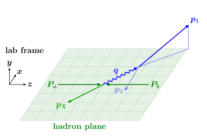
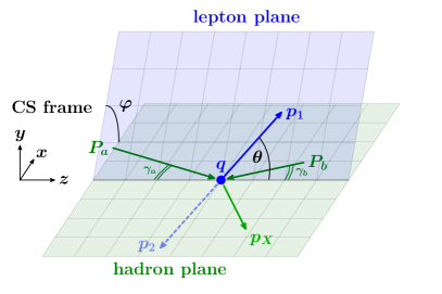
Figure -659: Kinematics in the lab frame (left) and the Collins-Soper frame (right). In the lab frame, the incoming hadron momenta are head-to-head (assuming the lab frame and hadronic center-of-mass frame coincide), while the vector boson has nonvanishing three-momentum $\vec{q}$. The scattering $p(P_{a})\,p(P_{b})\to V(q)\,X(p_{X})$ defines the hadron plane (green). In the CS frame (right), the vector boson is at rest. The leptons are produced back to back in the lepton plane (blue). The magnitudes of the hadron momenta in general differ for $Y\neq 0$, but their angles $\gamma_{a,b}$ with respect to the $z$ axis (indicated by the double arcs) become equal in the limit of vanishing hadron masses. The Collins-Soper angles $\theta$ and $\varphi$ are defined as indicated.

In this subsection, we discuss the leptonic decay in more detail. For the most part, we specifically consider the leading-order Drell-Yan decays

$$Z/\gamma^{\ast}(q) \to\ell^{-}(p_{1})\,\ell^{+}(p_{2})\,,\qquad Z \to\nu(p_{1})\,\bar{\nu}(p_{2})\,,$$

$$\,\quad W^{+}(q) \to\nu_{\ell}(p_{1})\,\ell^{+}(p_{2})\,,\quad W^{-}(q) \to\ell^{-}(p_{1})\,\bar{\nu}_{\ell}(p_{2})\,,$$ (2.54)

neglecting lepton masses, $m_{1,2}=0$, and summing over lepton polarizations. These are the primary application we are eventually interested in. The kinematics of the process in the lab and CS frames are illustrated in the left and right panels of figure -659.

In section 2.4.4, we discuss the extension to more complicated leptonic final states, e.g. including QED final-state radiation, which is important at the precision of current Drell-Yan measurements. In particular, there we show to what extent the LO discussion carries over for measurements that are performed in terms of suitably defined Born leptons.

2.4.1 Definition of CS angles

It is convenient to introduce spherical coordinates $(\cos\theta,\varphi)$ in the CS frame, in terms of which we can parametrize $p_{1,2}$, as illustrated in the right panel of figure -659, as

$$p_{1,2}^{\mu}=\frac{Q}{2}\Bigl{(}t^{\mu}\pm x^{\mu}\sin\theta\cos\varphi\pm y^{\mu}\sin\theta\sin\varphi\pm z^{\mu}\cos\theta\Bigr{)}\,.$$ (2.55)

The angles $\theta,\varphi$ are known as Collins-Soper angles. From eq. (2.55), one can easily derive their explicit expressions in terms of lab-frame quantities $E_{1,2}$, $p_{1,2}^{x,y,z}$,

$$\cos\theta =\frac{1}{Qm_{T}}\bigl{[}(E_{1}+p_{1}^{z})(E_{2}-p_{2}^{z})-(E_{1}-p_{1}^{z})(E_{2}+p_{2}^{z})\bigr{]}\,,$$

$$\cos\varphi =\frac{1}{\sin\theta}\frac{p_{1T}^{2}-p_{2T}^{2}}{q_{T}m_{T}}\,,\qquad\sin\varphi=\frac{2}{\sin\theta}\frac{p_{1}^{y}p_{2}^{x}-p_{2}^{y}p_{1}^{x}}{q_{T}Q}\,,$$ (2.56)

Note that we have arbitrarily chosen the positive orientation of the $z$ axis by having hadron $a$ move in the $z$ direction in the lab frame. As a result, the negatively charged lepton moves into the same rest-frame hemisphere as hadron $a$ for $\cos\theta>0$. In experimental measurements at the LHC, where the choice of $a$ and $b$ is arbitrary, hadron $b$ is often taken to be the one closer to the vector boson in rapidity to ensure that angular distributions do not average out when integrating over rapidity, see e.g. refs. [3, 11, 5, 14]. The resulting angles $\theta^{*}$ and $\varphi^{*}$, which are often also referred to as Collins-Soper angles, are then related to eq. (2.4.1) by

$$\cos\theta^{*}=\frac{Y}{\lvert Y\rvert}\cos\theta\,,\qquad\varphi^{*}=\frac{Y}{\lvert Y\rvert}\varphi\,.$$ (2.57)

On the other hand, eq. (2.4.1) does not depend on the chosen orientations of the $x$ and $y$ axes in the lab frame as long as they form a right-handed coordinate system.

The advantage of eq. (2.55), or equivalently the boost definition to define the CS frame, is that it stays true regardless of whether hadron masses are included or neglected, and thus also any relations like eq. (2.4.1) that are derived from it are independent of any beam parameters. On the other hand, with the bisector construction including hadron masses, eq. (2.4.1) no longer holds, see also the discussion in section 2.3.1.

2.4.2 Leptonic decay parametrization by angles

The fully-differential leptonic tensor for the $1\to 2$ Drell-Yan decays in eq. (2.4) at tree level has the form

$$L^{\mu\nu}(p_{1},p_{2}) =\frac{24\pi}{q^{2}}\Bigl{[}L_{+}(q^{2})\bigl{(}p_{1}^{\mu}p_{2}^{\nu}+p_{1}^{\nu}p_{2}^{\mu}-g^{\mu\nu}p_{1}\cdot p_{2}\bigr{)}+\mathrm{i}L_{-}(q^{2})\,\epsilon^{\mu\nu\rho\sigma}p_{1\rho}p_{2\sigma}\Bigr{]}\,.$$ (2.58)

Only the contribution proportional to $L_{+}$ ($L_{-}$) survives the contraction with the symmetric (antisymmetric) $P_{i}^{\mu\nu}$ corresponding to the parity-even (parity-odd) hadronic structure functions $W_{-1,0,1,2,5,6}$ ($W_{3,4,7}$). The normalization is chosen such that $L_{+}(q^{2})=L(q^{2})$ agrees with the inclusive coefficient in eq. (2.20), and such that $L_{-}(q^{2})=L_{+}(q^{2})$ for $W$ decays, where parity is maximally violated. Explicit expressions for the $L_{\pm}(q^{2})$ are given in appendix A.2.

It is convenient to parametrize the $2$-body decay phase space using the CS angles $\theta,\varphi$, in terms of which the phase-space measure is isotropic,

$$\mathrm{d}\Phi_{L}(q)=\frac{\mathrm{d}\cos\theta\,\mathrm{d}\varphi}{32\pi^{2}}\,.$$ (2.59)

Applying this parametrization to eq. (2.52), we find

$$L_{i}(q,\mathcal{O},\Theta) =\int_{-1}^{1}\!\mathrm{d}\cos\theta\,\int_{0}^{2\pi}\mathrm{d}\varphi\,L_{i}(q^{2},\theta,\varphi)\,\delta[\mathcal{O}-\hat{\mathcal{O}}(q,\theta,\varphi)]\,\hat{\Theta}(q,\theta,\varphi)\,,$$ (2.60)

$$L_{i}(q^{2},\theta,\varphi) =\frac{3}{16\pi}L_{\pm(i)}(q^{2})\,g_{i}(\theta,\varphi)\qquad\text{with}\qquad\pm\!(i)=\begin{cases}+\,,\qquad i\in\{-1,0,1,2,5,6\}\,,\\ -\,,\qquad i\in\{3,4,7\}\,,\end{cases}$$

where the angular dependence arises from contracting $P_{i}^{\mu\nu}$ with the Lorentz structures in eq. (2.58), and is encoded in nine (real combinations of) spherical harmonics

$$g_{-1}(\theta,\varphi) =1+\cos^{2}\theta\,,\qquad g_{2}(\theta,\varphi) =\tfrac{1}{2}\sin^{2}\theta\cos(2\varphi)\,,\qquad g_{5}(\theta,\varphi) =\sin^{2}\theta\sin(2\varphi)\,,$$

$$g_{0}(\theta,\varphi) =1-\cos^{2}\theta\,,\qquad g_{3}(\theta,\varphi) =\sin\theta\cos\varphi\,,\qquad g_{6}(\theta,\varphi) =\sin(2\theta)\sin\varphi\,,$$

$$g_{1}(\theta,\varphi) =\sin(2\theta)\cos\varphi\,,\qquad g_{4}(\theta,\varphi) =\cos\theta\,,\qquad g_{7}(\theta,\varphi) =\sin\theta\sin\varphi\,.$$ (2.61)

Putting everything together, we obtain

$$\frac{\mathrm{d}\sigma(\Theta)}{\mathrm{d}^{4}q\,\mathrm{d}\mathcal{O}} =\int_{-1}^{1}\!\mathrm{d}\cos\theta\,\int_{0}^{2\pi}\mathrm{d}\varphi\,\frac{\mathrm{d}\sigma}{\mathrm{d}^{4}q\,\mathrm{d}\cos\theta\,\mathrm{d}\varphi}\,\delta[\mathcal{O}-\hat{\mathcal{O}}(q,\theta,\varphi)]\,\hat{\Theta}(q,\theta,\varphi)\,,$$

$$\frac{\mathrm{d}\sigma}{\mathrm{d}^{4}q\,\mathrm{d}\cos\theta\,\mathrm{d}\varphi} =\frac{1}{2E_{\mathrm{cm}}^{2}}\sum_{i=-1}^{7}L_{i}(q^{2},\theta,\varphi)\,W_{i}(q^{2},s_{aq},s_{bq})\equiv\frac{3}{16\pi}\sum_{i=-1}^{7}\frac{\mathrm{d}\sigma_{i}}{\mathrm{d}^{4}q}\,g_{i}(\theta,\varphi)\,,$$ (2.62)

where in the last step we defined the so-called helicity cross sections

$$\frac{\mathrm{d}\sigma_{i}}{\mathrm{d}^{4}q}=\frac{1}{2E_{\mathrm{cm}}^{2}}L_{\pm(i)}(q^{2})\,W_{i}(q^{2},s_{aq},s_{bq})\,.$$ (2.63)

Integrating over $\mathcal{O}$ and setting $\hat{\Theta}=1$, we recover the inclusive cross section in eq. (2.21),

$$\frac{\mathrm{d}\sigma}{\mathrm{d}^{4}q}=\frac{\mathrm{d}\sigma_{-1}}{\mathrm{d}^{4}q}+\frac{1}{2}\frac{\mathrm{d}\sigma_{0}}{\mathrm{d}^{4}q}\,,\qquad W_{\mathrm{incl}}=W_{-1}+\frac{W_{0}}{2}\,.$$ (2.64)

2.4.3 Relation to angular coefficients

From eq. (2.4.2), we can write the fully-differential cross section in the CS angles as

$$\frac{\mathrm{d}\sigma}{\mathrm{d}^{4}q\,\mathrm{d}\cos\theta\,\mathrm{d}\varphi}=\frac{3}{16\pi}\frac{\mathrm{d}\sigma}{\mathrm{d}^{4}q}\biggl{[}1+\cos^{2}\theta+\frac{A_{0}}{2}\bigl{(}1-3\cos^{2}\theta\bigr{)}+\sum_{i=1}^{7}A_{i}\,g_{i}(\theta,\varphi)\biggr{]}\,,$$ (2.65)

where the angular coefficients $A_{i}$ are given in terms of the helicity cross sections or the hadronic structure functions as

$$A_{i} =\frac{\mathrm{d}\sigma_{i}}{\mathrm{d}\sigma_{-1}+\frac{1}{2}\mathrm{d}\sigma_{0}} =\frac{L_{\pm(i)}(q^{2})\,W_{i}(q^{2},s_{aq},s_{bq})}{L_{+}(q^{2})\,(W_{-1}+\frac{1}{2}W_{0}\bigr{)}(q^{2},s_{aq},s_{bq})}\,.$$ (2.66)

We deliberately chose the numbering and normalization of the $W_{i}$ in eq. (2.3.2) to match the often used form of the cross section in eq. (2.65). The only exception is the inclusive cross section, which is split into orthogonal contributions from $W_{0}$ and $W_{-1}$. For the same reason, we refrained from normalizing the spherical harmonics in eq. (2.4.2). We remind the reader that both numerator and denominator in eq. (2.66) in general involve a sum over the intermediate vector bosons, $L_{\pm}W_{i}\equiv\sum_{V,V^{\prime}}L_{\pm VV^{\prime}}W_{i\,VV^{\prime}}$ so for neutral-current Drell-Yan ($V=Z,\gamma$), the parity-even leptonic prefactors $L_{+}(q^{2})\equiv L_{+VV^{\prime}}(q^{2})$ do not in general cancel in the ratio in eq. (2.66).

A priori, eq. (2.4.2) or eq. (2.65) simply provide a convenient way to parametrize the fully-differential Drell-Yan cross section for massless $2$-body decays. For this purpose, it is irrelevant whether or not the CS angles can be reconstructed experimentally. Similarly, the choice of the CS tensor decomposition is a priori arbitrary, and we could have used another decomposition. Of course, the combination of using the CS tensor decomposition for the hadronic tensor together with using the CS angles to parametrize the leptonic tensor is what leads to the simple angular dependence in eq. (2.4.2). If we were to choose a different tensor decomposition $W_{i}^{\prime}$, we would also choose polar coordinates $\cos\theta^{\prime}$, $\varphi^{\prime}$ with respect to its corresponding rest frame, and arrive at eqs. (2.65) and (2.66) in terms of $\cos\theta^{\prime}$, $\varphi^{\prime}$, $A_{i}^{\prime}$, and $W_{i}^{\prime}$. On the other hand, when $\cos\theta$ and $\varphi$ are explicitly measured, or when eq. (2.65) is used as a template to measure the $A_{i}$, it obviously does matter with respect to which frame they are defined. It is also straightforward to relate the $W_{i}$ or $A_{i}$ for different frames, see section 2.6 below.

2.4.4 Extension to more complicated leptonic final states

Up to now, our discussion in this subsection assumed the leading-order dilepton final states in eq. (2.4), and so in particular eq. (2.65) is derived in this limit. For a generic leptonic final state $L$, e.g. when including QED final-state radiation (FSR) or for more complicated electroweak decays like $V^{*}\to VH$ or $V^{*}\to V_{1}V_{2}$, there is a priori no reason that the $L_{i}$ are proportional to spherical harmonics $g_{i}(\theta,\varphi)$ any longer, in which case one cannot use eq. (2.65) to define the $A_{i}$ beyond this LO.

On the other hand, as we saw in eq. (2.66), the $A_{i}$ are in one-to-one correspondence with the underlying hadronic structure functions $W_{i}$. The $W_{i}$ are by construction independent of $L$ (apart from its total momentum $q^{\mu}$) and thus well-defined for arbitrary $L$. The physical reason for the appearance of nine independent structures in both cases is exactly the same, namely the spin-1 nature of the intermediate vector boson (and the fact that we ignore the non-conserved parts). Hence, the cross section in the CS tensor decomposition in eq. (2.53) should be considered as the generalization of the LO angular decomposition in eq. (2.65) to arbitrary leptonic final states and measurements. One could also use eq. (2.66) as the all-order definition of the $A_{i}$ in terms of the $W_{i}$ and conventional LO weak couplings and propagators included in the $L_{\pm}(q^{2})$. One could then easily rewrite eq. (2.53) in terms of the so-defined $A_{i}$ multiplied by generic leptonic coefficients $L_{i}(q,\mathcal{O},\Theta)$, which in the simplest case reduce to $L_{\pm}(q^{2})g_{i}(\theta,\varphi)$ as in eq. (2.60), but in general can also be more complicated. Although at that point, it is easier and perhaps less confusing to directly work in terms of the $W_{i}$ and eq. (2.53) as it is.

Nevertheless, in the context of Drell-Yan measurements, the LO relation in eq. (2.65) is very useful in practice because the $g_{i}$ are orthogonal spherical harmonics. This allows one to directly measure the $A_{i}$ (or $W_{i}$) by performing a fit to the angular dependence of the $(\theta,\varphi)$ distribution or by projecting out different terms by taking suitably weighted angular integrals of it [11, 5]. This procedure has received some criticism, since it seemingly relies on a LO QED interpretation of the angular dependence, while QED final-state radiation can be relevant at the level of precision reached by Drell-Yan measurements. In fact, even the definition of the CS angles $(\theta,\varphi)$ themselves becomes nonobvious, because with additional QED radiation in the final state, the lepton momenta generically no longer add to the full vector-boson momentum $q^{\mu}$. Instead, we now have

$$q^{\mu}=p_{1}^{\mu}+p_{2}^{\mu}+k^{\mu}\,,$$ (2.67)

where $p^{\mu}_{1,2}$ are the measured lepton momenta, which depend on the lepton definition, and $k^{\mu}$ is the remaining momentum not included in the definitions of $p_{1,2}$. We stress that here we are not concerned with the experimental methods to reconstruct and calibrate the leptons or to recover photon radiation. The “measured” lepton momenta $p_{1,2}^{\mu}$ refer to the truth-level lepton definition to which the raw reconstructed momenta are corrected or unfolded. This truth-level definition must be theoretically well-defined to have a meaningful measurement that can be compared to theoretical calculations, and one can consider the question whether certain truth-level definitions are theoretically preferred or not.

Obviously, the $(\theta_{1},\varphi_{1})$ angles describing the orientation of $p_{1}$ now depend on the lepton definition and also on whether they are defined in the full vector-boson rest frame (where $q^{\mu}$ or equivalently the full $L$ is at rest) or the dilepton rest frame (where only $p_{1}^{\mu}+p_{2}^{\mu}$ is at rest). Especially in the latter case, there is no guarantee (in fact it seems quite unlikely) that the angular distribution in $(\theta_{1},\varphi_{1})$ will still admit a decomposition in terms of the nine spherical harmonics $g_{i}(\theta_{1},\varphi_{1})$.

For “bare” leptons, $p_{1,2}^{\mu}$ are defined without including any FSR photons. This means infrared QED singularities are regulated by the lepton mass leading to potentially large logarithms of the lepton mass. This effect is reduced by defining “dressed” leptons, which include all photons radiated within a cone of some size around the leptons, and hence can be theoretically thought of as QED “lepton jets”. With either definition, the remaining momentum $k^{\mu}$ in eq. (2.67) is nonzero and so the dilepton and vector-boson rest frames are no longer equivalent.

Another option is to include all $k^{\mu}$ into $p_{1,2}^{\mu}$, i.e., the lepton momenta are (partially) defined by the condition $q^{\mu}=p_{1}^{\mu}+p_{2}^{\mu}$. This is basically what “Born” leptons are. Their full definition corresponds to defining an IR-safe projection of the full leptonic final state $L$ onto a Born-like $2$-body final state. In principle there are many ways to do so, but as long as the Born projection is well defined so are the Born leptons.

To illustrate this, let us consider an explicit example: We start by defining the leptonic thrust axis $\vec{n}_{L}$ of the full leptonic final state $L$ in its rest frame. The thrust axis $\vec{n}_{L}$ is defined in the usual way as the axis $\vec{n}$, with $\vec{n}^{2}=1$, that minimizes

$$\vec{n}_{L}:\qquad\min_{\vec{n}}\sum_{i\in L}(E_{i}-|\vec{n}\cdot\vec{p}_{i}|)=Q-\max_{\vec{n}}\sum_{i}|\vec{n}\cdot\vec{p}_{i}|\,,$$ (2.68)

where the sum runs over all particles in $L$, including in particular all QED FSR, and $E_{i}$, $\vec{p}_{i}$ are defined in the rest frame of $L$. The overall positive (negative) orientation of $\vec{n}_{L}$ can be fixed by convention, e.g., to point into the hemisphere that contains the lepton (antilepton). Imposing the condition $p_{1}^{\mu}+p_{2}^{\mu}=q^{\mu}$, requiring massless on-shell momenta, $p_{1,2}^{2}=0$, and using $\vec{n}_{L}$ to define the direction of $\vec{p}_{1}=-\vec{p}_{2}$, then uniquely determines (recall $Q=\sqrt{q^{2}}$)

$$p_{1,2}^{\mu}=\frac{Q}{2}\,(1,\pm\vec{n}_{L})_{\mathrm{CS}}\equiv\frac{Q}{2}(t^{\mu}\pm n_{L}^{\mu})\,.$$ (2.69)

In the second step we defined the unit vectors

$$t^{\mu}=\frac{q^{\mu}}{Q}=(1,\vec{0})_{\mathrm{CS}}\,,\qquad n_{L}^{\mu}=(0,\vec{n}_{L})_{\mathrm{CS}}\,,\quad n_{L}^{2}=-1\,,\qquad t\cdot n_{L}=0\,,$$ (2.70)

where $t^{\mu}$ is the same as before, and $n_{L}^{\mu}$ describes the overall orientation of $L$.

More generally, we can also carry out the construction in two steps, first constructing $q^{\mu}=P_{1}^{\mu}+P_{2}^{\mu}$ with massive $P_{1,2}^{2}\neq 0$ and then projecting them onto massless $p_{1,2}$. Here, we first cluster all emissions with either the lepton or antilepton based on whose hemisphere they are in, which yields the massive hemisphere momenta $P_{1,2}^{\mu}$,

$$P_{1,2}^{\mu} =\frac{Q}{2}\bigl{[}x_{1,2}\,t^{\mu}\pm\lambda(q^{2},P_{1}^{2},P_{2}^{2})\,n_{L}^{\mu}\bigr{]}\,,$$

$$x_{1,2} =1+\frac{P_{1,2}^{2}-P_{2,1}^{2}}{q^{2}}\,,\qquad\lambda(q^{2},P_{1}^{2},P_{2}^{2})=\frac{1}{q^{2}}\sqrt{(q^{2}-P_{1}^{2}-P_{2}^{2})^{2}-4P_{1}^{2}P_{2}^{2}}\,.$$ (2.71)

Next, we project $P_{1,2}^{\mu}$ onto massless momenta $p_{1,2}^{\mu}$ by preserving the three-momentum direction, $\vec{p}_{1}/\lvert\vec{p}_{1}\rvert=\vec{P}_{1}/\lvert\vec{P}_{1}\rvert=\vec{n}_{L}$, and the total energy, $p_{1}^{0}+p_{2}^{0}=P_{1}^{0}+P_{2}^{0}=Q$, which yields eq. (2.69). The spherical coordinates $(\theta_{L},\varphi_{L})$ of $\vec{n}_{L}$ in the CS frame now provide a unique, all-order definition of the CS angles $(\theta,\varphi)\equiv(\theta_{L},\varphi_{L})$, i.e.,

$$n_{L}^{\mu}=x^{\mu}\sin\theta\cos\varphi+y^{\mu}\sin\theta\sin\varphi+z^{\mu}\cos\theta\,.$$ (2.72)

This is the generalization of eq. (2.55), where the CS angles now describe the overall orientation of $L$ in the CS frame, as illustrated in figure -658.

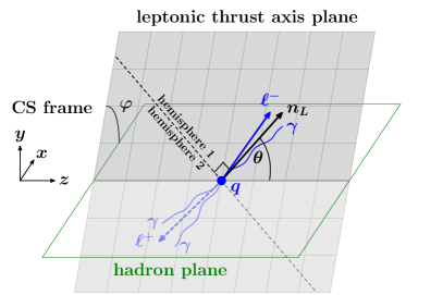
Figure -658: Definition of the Collins-Soper angles $\theta,\varphi$ for a generic leptonic final state including FSR (blue) in terms of the leptonic thrust axis $n_{L}$. The leptonic thrust axis plane in the CS frame is spanned by the $z$ axis and $n_{L}$ and generalizes the lepton plane in figure -659. Beyond LO in QED, the decay products do no longer have to lie in this plane. The hadronic scattering in the hadron plane (green) is as in figure -659 and omitted for clarity. The hemisphere boundary (dashed line) is perpendicular to the thrust axis and separates the emissions into hemisphere 1 (clustered with the lepton) and hemisphere 2 (clustered with the antilepton).

It is easy to see that the above definitions are IR safe and reduce to the respective LO definitions. In principle, any other IR-safe way of clustering the emissions into $P_{1,2}^{\mu}$ is possible. Other ways to project them onto massless $p_{1,2}^{\mu}$ are also possible, as long as the projection is IR safe and preserves the total leptonic momentum $q^{\mu}=P_{1}^{\mu}+P_{2}^{\mu}=p_{1}^{\mu}+p_{2}^{\mu}$. In practice, defining the projection by keeping the orientation fixed is the most natural and also the easiest, as it avoids any confusion about which particular direction is used to define the CS angles.

The advantage of Born leptons is that they do admit an analogous LO-like angular decomposition as we will now show. More generally, it is sufficient to restrict to leptonic measurements that can be written in terms of $P_{1,2}^{\mu}$,

$$\hat{\mathcal{O}}(q,\Phi_{L}) \equiv\hat{\mathcal{O}}(q,P_{1},P_{2})=\hat{\mathcal{O}}(q,\theta,\varphi,P_{1}^{2},P_{2}^{2})\,,$$

$$\hat{\Theta}(q,\Phi_{L}) \equiv\hat{\Theta}(q,P_{1},P_{2})=\hat{\Theta}(q,\theta,\varphi,P_{1}^{2},P_{2}^{2})\,.$$ (2.73)

For such measurements we can write the general leptonic tensor in eq. (2.1) as

$$L^{\mu\nu}(q,\mathcal{O},\Theta) =\int\!\frac{\mathrm{d}^{4}P_{1}}{(2\pi)^{3}}\,\frac{\mathrm{d}^{4}P_{2}}{(2\pi)^{3}}\,(2\pi)^{4}\delta^{4}(q-P_{1}-P_{2})\,F^{\mu\nu}(P_{1},P_{2})$$

$$\qquad\times\delta[\mathcal{O}-\hat{\mathcal{O}}(q,P_{1},P_{2})]\,\hat{\Theta}(q,P_{1},P_{2})\,,$$ (2.74)

where $F^{\mu\nu}(P_{1},P_{2})$ is the projection of the full leptonic decay $L^{\mu\nu}(\Phi_{L})$ onto the massive $2$-body $(P_{1},P_{2})$ phase space,

$$F^{\mu\nu}(P_{1},P_{2}) =(2\pi)^{2}\int\!\mathrm{d}\Phi_{L}(P_{1}+P_{2})\,L^{\mu\nu}(\Phi_{L})\,\delta^{4}[P_{1}-\hat{P}(\Phi_{L})]\,,$$ (2.75)

where $\hat{P}^{\mu}(\Phi_{L})$ implements the clustering of $\Phi_{L}$ into $P_{1}^{\mu}$, and $P_{2}^{\mu}$ is implicitly defined via $q^{\mu}=P_{1}^{\mu}+P_{2}^{\mu}$. For the LO decays in eq. (2.4), we have $\Phi_{L}=(p_{1},p_{2})$ and $\hat{P}(\Phi_{L})=p_{1}$ such that

$$F_{\rm LO}^{\mu\nu}(P_{1},P_{2})=L^{\mu\nu}(P_{1},P_{2})\,\delta(P_{1}^{2})\,\delta(P_{2}^{2})\,,$$ (2.76)

with $L^{\mu\nu}(p_{1},p_{2})$ given by the LO result in eq. (2.58).

The key point is that $F^{\mu\nu}(P_{1},P_{2})$ is defined in a Lorentz-covariant way, and therefore obeys the following Lorentz decomposition (ignoring as before the non-conserved parts)

$$F^{\mu\nu}(P_{1},P_{2}) =12\pi\Bigl{[}(t^{\mu}t^{\nu}-g^{\mu\nu}-n_{L}^{\mu}n_{L}^{\nu})\,F_{+}+(t^{\mu}t^{\nu}-g^{\mu\nu})\,F_{0}+\mathrm{i}\epsilon^{\mu\nu\rho\sigma}n_{L\rho}t_{\sigma}\,F_{-}\Bigr{]}$$

$$\qquad\text{($+$ terms $\propto q^{\mu}$ or $q^{\nu}$)}\,,$$ (2.77)

where $F_{\pm,0}\equiv F_{\pm,0}(q^{2},P_{1}^{2},P_{2}^{2})$ are Lorentz-scalar functions that can only depend on three independent invariants formed out of $P_{1,2}$, which we chose as $q^{2}=(P_{1}+P_{2})^{2}$ and $P_{1,2}^{2}$. The decomposition in eq. (2.4.4) is chosen so that at LO, comparing to eq. (2.58), we have

$$F_{\pm}(q^{2},P_{1}^{2},P_{2}^{2}) =L_{\pm}(q^{2})\,\delta(P_{1}^{2})\delta(P_{2}^{2})+\mathcal{O}(\alpha_{\mathrm{em}})\,,\qquad F_{0}(q^{2},P_{1}^{2},P_{2}^{2})=\mathcal{O}(\alpha_{\mathrm{em}})\,.$$ (2.78)

The leptonic structure functions are now obtained as defined in eq. (2.52), by contracting eq. (2.4.4) with the projectors $P_{i}^{\mu\nu}$ and performing the phase-space integrals in eq. (2.4.4),

$$L_{i}(q,\mathcal{O},\Theta) =\int\!\mathrm{d}\cos\theta\,\mathrm{d}\varphi\,\mathrm{d}P_{1}^{2}\,\mathrm{d}P_{2}^{2}\,\lambda(q^{2},P_{1}^{2},P_{2}^{2})\,L_{i}(q^{2},\theta,\varphi,P_{1}^{2},P_{2}^{2})$$

$$\qquad\times\delta\bigl{[}\mathcal{O}-\hat{\mathcal{O}}(q,\theta,\varphi,P_{1}^{2},P_{2}^{2})\bigr{]}\,\hat{\Theta}(q,\theta,\varphi,P_{1}^{2},P_{2}^{2})\,,$$ (2.79)

with the underlying leptonic structure functions given by

$$L_{-1}(q^{2},\theta,\varphi,P_{1}^{2},P_{2}^{2}) =\frac{3}{16\pi}\Bigl{[}F_{+}(q^{2},P_{1}^{2},P_{2}^{2})\,g_{-1}(\theta,\varphi)+2F_{0}(q^{2},P_{1}^{2},P_{2}^{2})\Bigr{]}\,,$$

$$L_{0}(q^{2},\theta,\varphi,P_{1}^{2},P_{2}^{2}) =\frac{3}{16\pi}\Bigl{[}F_{+}(q^{2},P_{1}^{2},P_{2}^{2})\,g_{0}(\theta,\varphi)+F_{0}(q^{2},P_{1}^{2},P_{2}^{2})\Bigr{]}\,,$$

$$L_{1,2,5,6}(q^{2},\theta,\varphi,P_{1}^{2},P_{2}^{2}) =\frac{3}{16\pi}F_{+}(q^{2},P_{1}^{2},P_{2}^{2})\,g_{1,2,5,6}(\theta,\varphi)\,,$$

$$L_{3,4,7}(q^{2},\theta,\varphi,P_{1}^{2},P_{2}^{2}) =\frac{3}{16\pi}F_{-}(q^{2},P_{1}^{2},P_{2}^{2})\,g_{3,4,7}(\theta,\varphi)\,.$$ (2.80)

Eqs. (2.4.4) and (2.4.4) are the generalization of eq. (2.60) to an arbitrary Born-projected leptonic final state $L$. The $(\theta,\varphi)$ dependence is still completely described by the same $g_{i}(\theta,\varphi)$ in eq. (2.4.2). The $L_{i}$ for $i\geq 1$ are still given by their own respective $g_{i}$ times a common leptonic form factor $F_{+}$ for $i=1,2,5,6$ and $F_{-}$ for $i=3,4,7$. On the other hand, the angular dependence of $L_{-1}$ and $L_{0}$ now gets mixed up by $F_{0}$, which enters with a flat $(\theta,\varphi)$ dependence corresponding to $g_{-1}+g_{0}=2$.

If the measurements are defined in terms of massless Born leptons, then they are also independent of $P_{1,2}^{2}$, such that the $P_{1,2}^{2}$ integrals in eq. (2.4.4) can be performed to give $L_{i}(q^{2},\theta,\varphi)$ that are given by the same expressions as in eq. (2.4.4) but in terms of corresponding integrated

$$F_{\pm,0}(q^{2})=\int\!\mathrm{d}P_{1}^{2}\,\mathrm{d}P_{2}^{2}\,\lambda(q^{2},P_{1}^{2},P_{2}^{2})\,F_{\pm,0}(q^{2},P_{1}^{2},P_{2}^{2})\,.$$ (2.81)

Removing all leptonic measurements, the inclusive $q_{T}$ spectrum is now given by

$$\frac{\mathrm{d}\sigma}{\mathrm{d}^{4}q}=\frac{1}{2E_{\mathrm{cm}}^{2}}\Bigl{[}F_{+}(q^{2})+\frac{3}{2}F_{0}(q^{2})\Bigr{]}W_{\mathrm{incl}}(q^{2},s_{aq},s_{bq})\,,\qquad W_{\mathrm{incl}}=W_{-1}+\frac{W_{0}}{2}\,,$$ (2.82)

i.e., in terms of the same inclusive hadronic structure function multiplied by a generalized inclusive leptonic function. We remind the reader that also here there is always an implicit sum over intermediate vector bosons, $F_{\pm,0}W_{i}\equiv\sum_{V,V^{\prime}}F_{\pm,0\,VV^{\prime}}W_{i\,VV^{\prime}}$. The cross section differential in the CS angles becomes

$$\frac{\mathrm{d}\sigma}{\mathrm{d}^{4}q\,\mathrm{d}\cos\theta\,\mathrm{d}\varphi} =\frac{1}{2E_{\mathrm{cm}}^{2}}\frac{3}{16\pi}\biggl{[}2F_{0}\,W_{\mathrm{incl}}+\sum_{i=-1}^{7}F_{\pm(i)}W_{i}\,g_{i}(\theta,\varphi)\biggr{]}$$ (2.83)

$$=\frac{1}{2E_{\mathrm{cm}}^{2}}\frac{3}{16\pi}\biggl{[}\Bigl{(}F_{+}\!+\frac{3}{2}F_{0}\Bigr{)}W_{\mathrm{incl}}(1+\cos^{2}\theta)+\frac{F_{+}W_{0}+F_{0}\,W_{\mathrm{incl}}}{2}\,\bigl{(}1-3\cos^{2}\theta\bigr{)}$$

$$\qquad\qquad\qquad+\sum_{i=1}^{7}F_{\pm(i)}W_{i}\,g_{i}(\theta,\varphi)\biggr{]}$$

$$\equiv\frac{\mathrm{d}\sigma}{\mathrm{d}^{4}q}\biggl{[}1+\cos^{2}\theta+\frac{\tilde{A}_{0}}{2}\,\bigl{(}1-3\cos^{2}\theta\bigr{)}+\sum_{i=1}^{7}\tilde{A}_{i}\,g_{i}(\theta,\varphi)\biggr{]}\,,$$

where we suppressed the arguments of the structure functions for brevity, and the analogous expression also holds differential in $P_{1,2}^{2}$. To make contact with eq. (2.65), in the second step we split the flat contribution from $F_{0}$ as $(3/2)(1+\cos^{2}\theta)+(1/2)(1-3\cos^{2}\theta)=2$, and in the last step we factored out the inclusive cross section in eq. (2.82), denoting the resulting normalized coefficients of the angular dependence as $\tilde{A}_{i}$,

$$\tilde{A}_{0}=\frac{F_{+}\,W_{0}+F_{0}\,W_{\mathrm{incl}}}{\bigl{(}F_{+}+\tfrac{3}{2}F_{0}\bigr{)}\,W_{\mathrm{incl}}}\,,\qquad\tilde{A}_{i\geq 1}=\frac{F_{\pm(i)}W_{i}}{\bigl{(}F_{+}+\tfrac{3}{2}F_{0}\bigr{)}\,W_{\mathrm{incl}}}\,.$$ (2.84)

These are the generalization of the $A_{i}$ in eq. (2.66) for an arbitrary Born-projected final state. They implicitly depend on the specific Born projection used because the CS angles $(\theta,\varphi)$ implicitly depend on it. The $\tilde{A}_{i}$ are the angular coefficients that are measured by decomposing or projecting the $(\theta,\varphi)$ dependence defined in terms of Born-projected leptons. It would be interesting to precisely identify the underlying Born projection that is effectively used in the measurements [11, 5].

Generically, the QED corrections to $F_{+}$, $F_{-}$, and $F_{0}$ will differ and thus not cancel in eq. (2.84). In other words, even though Born-projected leptons admit a well-defined LO-like angular decomposition as shown in eq. (2.83), the resulting $\tilde{A}_{i}$ in eq. (2.84) still differ by QED FSR corrections from the LO $A_{i}$ in eq. (2.66). These corrections should be of generic $\mathcal{O}(\alpha_{\mathrm{em}})$ size, i.e., neither enhanced by soft or collinear photon emissions nor suppressed near the $Z$ pole. In the limit of an on-shell $Z$ boson, they would produce the QED corrections to the $Z$ decay rate to leptons. For $i\geq 1$, the hadronic contributions to $A_{i}$ and $\tilde{A}_{i}$ are the same. As we will discuss below, $W_{0}$ is suppressed by $\mathcal{O}(q_{T}^{2}/Q^{2})$ relative to $W_{\mathrm{incl}}$ at small $q_{T}$, such that at LO in QED $A_{0}$ vanishes like $q_{T}^{2}$ for $q_{T}\to 0$. Interestingly, $\tilde{A}_{0}$ receives an additional contribution $F_{0}\,W_{\mathrm{incl}}$, and therefore it no longer vanishes for $q_{T}\to 0$ but goes to a calculable $\mathcal{O}(\alpha_{\mathrm{em}})$ constant.

Ref. [139] considered QED radiation off massive final-state leptons, and found linear power corrections even in the inclusive case. Since their massive leptons correspond to bare leptons, this is not entirely surprising. It would be interesting to identify the precise source of linear power corrections, i.e, whether the bare leptons induce linear corrections in the leptonic tensor itself, or populate additional leptonic structure functions that come with linearly suppressed hadronic structure functions, or both.

Finally, while most of the above discussion was phrased in terms of QED FSR corrections to Drell-Yan, it applies to an arbitrary Born-projected final state $L$. For example, keeping the $P_{1,2}^{2}$ dependence, it applies to Drell-Yan-like electroweak diboson production $V^{*}\to VH$ or $V^{*}\to V_{1}V_{2}$ if one remains inclusive over the decays of the final-state bosons.

2.5 Factorization for fiducial power corrections

We now investigate the structure of power corrections in the limit $q_{T}\ll Q$ in the presence of measurements on the leptonic final state. To expand in $q_{T}\ll Q$, we introduce a formal power-counting parameter

$$\lambda\sim q_{T}/Q\,.$$ (2.85)

The leptonic measurements $\hat{\mathcal{O}}$ and $\hat{\Theta}$ in eq. (2.52) are functions of the total four-momentum $q$ of the final state, and admit an expansion in $\lambda$ as

$$\hat{\mathcal{O}}(q,\Phi_{L}) =\hat{\mathcal{O}}^{(0)}(q,\Phi_{L})\bigl{[}1+\mathcal{O}(\lambda)\bigr{]}\,,$$

$$\hat{\Theta}(q,\Phi_{L}) =\hat{\Theta}^{(0)}(q,\Phi_{L})\bigl{[}1+\mathcal{O}(\lambda)\bigr{]}\,.$$ (2.86)

We refer to the corrections in $\lambda$ in these expansions as fiducial power corrections. For observables that exist at Born level, e.g., cuts on the lepton momenta, the leading-power (LP) observables $\hat{\mathcal{O}}^{(0)}$ and $\hat{\Theta}^{(0)}$ are simply obtained by taking the Born limit $q_{T}\to 0$. For $q_{T}$-like resolution variables like $\phi^{*}$ that scale like $q_{T}$ itself and vanish at Born level, $\hat{\mathcal{O}}^{(0)}$ or $\hat{\Theta}^{(0)}$ are given by the leading, nontrivial contribution in the $q_{T}\to 0$ limit.

2.5.1 Linear fiducial power corrections

We first assume that the leptonic measurement does not induce any additional nontrivial dynamic scale $p_{L}$, such that the power expansion in eq. (2.5) is genuinely an expansion in $q_{T}/Q$. We can then focus on the linear $\mathcal{O}(\lambda)$ fiducial power corrections.

Let us consider leptonic measurements that are azimuthally symmetric at leading power, which we will indicate by $L^{(0)}(/\!\!\!\!\varphi)$ and define more precisely in a moment. We will show that for such measurements the only linear $\mathcal{O}(\lambda)$ power corrections that arise are due to the linear fiducial power corrections in eq. (2.5). As a result, the $\mathcal{O}(\lambda)$ power corrections can be uniquely predicted and resummed in terms of leading-power hadronic structure functions.

For measurements that can be parameterized in terms of CS angles $\theta$, $\varphi$, which includes our default Drell-Yan cases in eq. (2.4), azimuthal symmetry means that they do not depend on $\varphi$. Azimuthal symmetry at leading power then simply means that the LP measurements $\hat{\mathcal{O}}^{(0)}(q,\theta)$ and $\hat{\Theta}^{(0)}(q,\theta)$ are $\varphi$ independent, which implies that they average out against $\cos(n\varphi)$ and $\sin(n\varphi)$,

$$L^{(0)}(/\!\!\!\!\varphi)\,:\qquad \int_{0}^{2\pi}\mathrm{d}\varphi\,e^{\mathrm{i}n\varphi}\,\delta[\mathcal{O}-\hat{\mathcal{O}}^{(0)}(q,\theta)]\,\hat{\Theta}^{(0)}(q,\theta)=0\,,\qquad(n\geq 1)\,.$$ (2.87)

In particular, the integration against all spherical harmonics $g_{i}(\theta,\varphi)$ in eqs. (2.60) and (2.4.2) vanishes, except for $i=-1,0,4$, which do not depend on $\varphi$. More generally, we define a generic leptonic measurement as azimuthally symmetric if it only contributes to $L_{-1,0,4}$, such that azimuthal symmetry at leading power is defined by

$$L^{(0)}(/\!\!\!\!\varphi)\,:\qquad L_{i}^{(0)}(q,\mathcal{O},\Theta)=0\,,\qquad i\neq-1,0,4\,.$$ (2.88)

Note that this definition is also natural from the point of view of the CS tensor decomposition in eq. (2.3.2). Azimuthal symmetry corresponds to symmetry under rotations of the $x$ and $y$ axes around the $z$ axis. The projections for $i=-1,0,4$ are precisely those that are invariant under azimuthal rotations (corresponding to the norm and cross product, or are independent of $x$ and $y$), which is the physical reason why their corresponding $g_{i}(\theta,\varphi)$ do not depend on $\varphi$.

A primary example is a fiducial cut on the lepton transverse momenta $p_{T1,2}\geq p_{T}^{\mathrm{min}}$, for which we have

$$\hat{\Theta}^{(0)}(Q,Y,{\vec{q}}_{T},\theta)=\theta\Bigl{(}p_{T}^{\mathrm{min}}\leq\frac{Q}{2}\sin\theta\Bigr{)}=\hat{\Theta}(Q,Y,{\vec{q}}_{T}=0,\theta,\varphi)\,.$$ (2.89)

In words, the leptons are exactly back-to-back at leading power, and whether they pass the cut only depends on their rest-frame energy $Q/2$ and scattering angle $\theta$. We discuss this case as well as a cut on the lepton rapidity in more detail in section 4.2. On the other hand, angular asymmetries that are designed to project out the $\cos\varphi$ or $\cos(2\varphi)$ dependence in the angular distribution (by construction) do not qualify under eq. (2.88).

Power expanding the leptonic structure functions, which includes the power expansion of the measurement, we have

$$L_{i}(q,\mathcal{O},\Theta) =L_{i}^{(0)}(q,\mathcal{O},\Theta)+L_{i}^{(1)}(q,\mathcal{O},\Theta)+\dotsb\,,$$ (2.90)

where with the assumption in eq. (2.88) only $L_{i}^{(0)}$ with $i=-1,0,4$ are nonzero. The $L_{i}^{(1)}$ contain the linear fiducial power corrections. They can be, and in general are, nonzero for other $i$, as our azimuthal symmetry assumption only concerns the leading-power $L_{i}^{(0)}$.

$W_{i}$	Scaling	$\pm(i)$	$g_{i}(\theta,\varphi)$	$L_{i}^{(0)}$
$W_{-1}$	$\sim\lambda^{0}$	$+$	$1+\cos^{2}\theta$	✓
$W_{0}$	$\sim\lambda^{2}$	$+$	$1-\cos^{2}\theta$	✓
$W_{1}$	$\sim\lambda^{1}$	$+$	$\sin(2\theta)\cos\varphi$	$-$
$W_{2}$	$\sim\lambda^{0}$	$+$	$\tfrac{1}{2}\sin^{2}\theta\cos(2\varphi)$	$-$
$W_{3}$	$\sim\lambda^{\geq 1}$	$-$	$\sin\theta\cos\varphi$	$-$
$W_{4}$	$\sim\lambda^{0}$	$-$	$\cos\theta$	✓
$W_{5}$	$\sim\lambda^{0}$	$+$	$\sin^{2}\theta\sin(2\varphi)$	$-$
$W_{6}$	$\sim\lambda^{\geq 1}$	$+$	$\sin(2\theta)\sin\varphi$	$-$
$W_{7}$	$\sim\lambda^{\geq 1}$	$-$	$\sin\theta\sin\varphi$	$-$

Table 1: Scaling of the hadronic structure functions $W_{i}$ in the CS tensor decomposition in eq. (2.3.2) in the limit $\lambda\sim q_{T}/Q\ll 1$ relative to the leading $W_{-1,4}\sim 1/q_{T}^{2}$. In this table we generically count $\Lambda_{\mathrm{QCD}}\sim q_{T}$. In several cases we only derive bounds on the scaling, where $\sim\lambda^{\geq m}$ means the $W_{i}$ is suppressed by at least $\lambda^{m}$. We group the structure functions by parity and whether they arise from the dispersive ($i=-1\dots 4$) or absorptive parts ($i=5\dots 7$) of the production amplitude [140]. The second-to-last column shows the corresponding angular dependence $g_{i}(\theta,\varphi)$ on the Collins-Soper angles for $2$-body decays, and in the last column we indicate whether there is a nonvanishing LP leptonic tensor $L_{i}^{(0)}$ for observables that are azimuthally symmetric at Born level.

We also need to power-count the hadronic structure functions $W_{i}$,

$$W_{i}=\sum_{m=0}^{\infty}W_{i}^{(m)}\,,\qquad W_{i}^{(m)}\sim\frac{\lambda^{m}}{q_{T}^{2}}\,.$$ (2.91)

The $\lambda$ scaling of the first nonzero contributions $W_{i}^{(m)}$ relative to the leading-power $W_{-1,4}^{(0)}\sim 1/q_{T}^{2}$ is summarized in table 1, and is derived more carefully using SCET in section 2.6. From table 1, we see that the only nonvanishing LP structure functions $W_{i}^{(0)}$ are for $i=-1,2,4,5$. The physical reason is that at LP, angular momentum conservation works the same way as at tree level, i.e., as in the collision of two massless partons with $p_{a}+p_{b}=q$, $p_{Ta}=p_{Tb}=q_{T}=0$. In this limit, the CS frame coincides with the leptonic frame, and the longitudinal polarization vector is given by

$$\varepsilon^{\mu}_{0}=\frac{p_{a}^{\mu}-p_{b}^{\mu}}{Q}\qquad\text{(tree level)}\,.$$ (2.92)

It is easy to see that projections of the tree-level partonic matrix element onto $\varepsilon^{\mu}_{0}$ vanish,

$$\varepsilon^{*}_{0\mu}\langle 0\lvert J_{\gamma}^{\mu}\rvert q(p_{a},s_{a})\bar{q}(p_{b},s_{b})\rangle\propto\bar{v}^{s_{b}}(p_{b})(p\!\!\!/_{a}-p\!\!\!/_{b})u^{s_{a}}(p_{a})=0$$ (2.93)

for any polarization $s_{a}$ ($s_{b}$) of the quark (antiquark), and similarly for the axial-vector current. It follows that structure functions $W_{i}$ that involve contractions with $\varepsilon^{\mu}_{0}$ vanish at tree level. We will see in section 2.6 that to all orders, each contraction with $\varepsilon^{\mu}_{0}$ is in fact penalized by at least one power of $\lambda$.

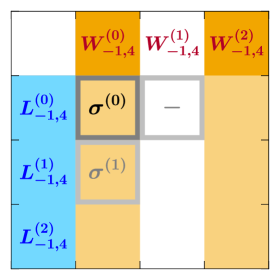
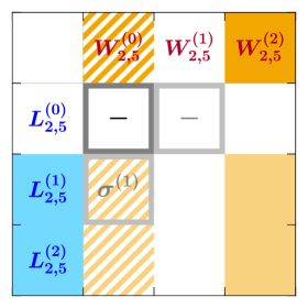
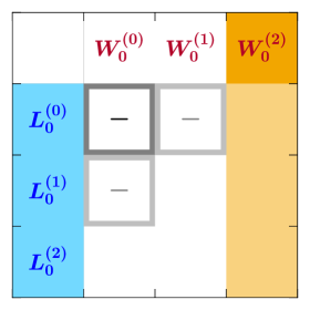
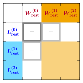
Figure -657: Power counting of hadronic structure functions and their leptonic counterparts for $\lambda\sim q_{T}/Q\ll 1$, assuming azimuthal symmetry at leading power. Nonzero contributions to the hadronic and leptonic tensors are indicated by solid orange and blue filling, respectively. Nonzero contributions to the cross section are indicated by solid light orange filling. Hatched filling for $W_{2,5}^{(0)}$ indicates that this contribution does not match onto leading-twist collinear PDFs and is suppressed for $\Lambda_{\mathrm{QCD}}\ll q_{T}$. Gray boxes indicate contributions to the LP and linear NLP cross sections $\sigma^{(0)}$ and $\sigma^{(1)}$. The latter solely arise through the leptonic tensor as $L_{i}^{(1)}W_{i}^{(0)}$ while all contributions of the form $L_{i}^{(0)}W_{i}^{(1)}$ vanish. Dashes indicate that a contribution vanishes. In the bottom right panel, “rest” refers to structure functions $i=1,3,6,7$.

Suppressing the arguments of $L_{i}$ and $W_{i}$, the strict LP cross section is given by

$$L^{(0)}(/\!\!\!\!\varphi)\,:\qquad\frac{\mathrm{d}\sigma^{(0)}(\Theta)}{\mathrm{d}^{4}q\,\mathrm{d}\mathcal{O}} =\frac{1}{2E_{\mathrm{cm}}^{2}}\sum_{i=-1,4}L_{i}^{(0)}\,W_{i}^{(0)}\,.$$ (2.94)

The $i=2,5$ contribution does not survive because $L_{2,5}^{(0)}=0$ due to eq. (2.88), and the nonzero $L_{0}^{(0)}$ does not contribute because $W_{0}^{(0)}=0$.

Next, the linear $\mathcal{O}(\lambda)$ power corrections to the cross section are given by

$$\frac{\mathrm{d}\sigma^{(1)}(\Theta)}{\mathrm{d}^{4}q\,\mathrm{d}\mathcal{O}} =\frac{1}{2E_{\mathrm{cm}}^{2}}\sum_{i=-1}^{7}\bigl{[}L_{i}^{(1)}\,W_{i}^{(0)}+L_{i}^{(0)}\,W_{i}^{(1)}\bigr{]}\,.$$ (2.95)

In the first term, only $i=-1,2,4,5$ contribute to the sum due to table 1. For the second term, assuming LP azimuthal symmetry, only $i=-1,0,4$ contribute. From table 1, $W_{0}\sim\mathcal{O}(\lambda^{2})$, and as we will argue in section 2.6, all power corrections to $W_{-1,4}$ are quadratic in $\lambda$, so we have

$$W_{-1}^{(1)}=0\,,\qquad W_{0}^{(1)}=0\,,\qquad W_{4}^{(1)}=0\,.$$ (2.96)

For $W_{-1}$ and $W_{0}$, this statement is equivalent to the absence of linear power corrections in the inclusive cross section $\propto W_{-1}+\frac{1}{2}W_{0}$. For $W_{4}$, it is equivalent to the absence of linear power corrections in the inclusive forward-backward asymmetry. Hence, the second term in eq. (2.95) vanishes, and we arrive at

$$L^{(0)}(/\!\!\!\!\varphi)\,:\qquad\frac{\mathrm{d}\sigma^{(1)}(\Theta)}{\mathrm{d}^{4}q\,\mathrm{d}\mathcal{O}} =\frac{1}{2E_{\mathrm{cm}}^{2}}\sum_{i=-1,2,4,5}L_{i}^{(1)}\,W_{i}^{(0)}\,.$$ (2.97)

We have thus shown that for leptonic measurements that are azimuthally symmetric at leading power, all linear power corrections uniquely arise from linear fiducial power corrections $L_{i}^{(1)}$ multiplying the leading-power hadronic structure functions $W_{-1,2,4,5}^{(0)}$. The power-counting logic leading to eq. (2.97) is illustrated in figure -657.

2.5.2 Leptonic fiducial power corrections

We now turn to leptonic fiducial power corrections that arise from the presence of an additional, physical scale $p_{L}$ induced by the leptonic measurement. In this case, the power expansion of the measurements a priori receives power corrections in both $q_{T}/Q$ and $q_{T}/p_{L}$,

$$\hat{\mathcal{O}}(q,\Phi_{L}) =\hat{\mathcal{O}}^{(0)}(q,\Phi_{L})\Bigl{[}1+\mathcal{O}\Bigl{(}\frac{q_{T}}{Q},\frac{q_{T}}{p_{L}}\Bigr{)}\Bigr{]}\,,$$

$$\hat{\Theta}(q,\Phi_{L}) =\hat{\Theta}^{(0)}(q,\Phi_{L})\Bigl{[}1+\mathcal{O}\Bigl{(}\frac{q_{T}}{Q},\frac{q_{T}}{p_{L}}\Bigr{)}\Bigr{]}\,.$$ (2.98)

The case of linear fiducial power corrections discussed above corresponds to $p_{L}\sim Q$. We refer to the $q_{T}/p_{L}$ corrections as leptonic fiducial power corrections. For $q_{T}\ll p_{L}\ll Q$, they become enhanced compared to the $q_{T}/Q$ corrections and for $q_{T}\sim p_{L}$ they become $\mathcal{O}(1)$ and cause the naive expansion in $q_{T}$ to break down.

Generically this happens when the leptonic measurement is close to an edge of Born phase space that is sensitive to additional radiation, such that a nonzero $q_{T}$ opens up new phase space beyond the Born edge, with $p_{L}\sim q_{T}$ parametrizing the distance from the Born edge. We will demonstrate this effect in detail in section 4.3 for the important example of the $p_{T}^{\ell}$ spectrum near the Jacobian peak $p_{T}^{\ell}\sim Q/2$, in which case $p_{L}=Q-2p_{T}^{\ell}$.

To expand in such regions, it is necessary to count both

$$\frac{q_{T}}{Q}\sim\frac{p_{L}}{Q}\sim\lambda\,,$$ (2.99)

which explicitly avoids expanding in $q_{T}/p_{L}\sim\mathcal{O}(1)$ and thereby retains all leptonic power corrections exactly to all powers. Expanding the leptonic measurements in this limit

$$\hat{\mathcal{O}}(q,\Phi_{L}) =\hat{\mathcal{O}}^{(0)}(q,\Phi_{L};q_{T}/p_{L})\Bigl{[}1+\mathcal{O}\Bigl{(}\frac{q_{T}}{Q},\frac{p_{L}}{Q}\Bigr{)}\Bigr{]}\,,$$

$$\hat{\Theta}(q,\Phi_{L}) =\hat{\Theta}^{(0)}(q,\Phi_{L};q_{T}/p_{L})\Bigl{[}1+\mathcal{O}\Bigl{(}\frac{q_{T}}{Q},\frac{p_{L}}{Q}\Bigr{)}\Bigr{]}\,,$$ (2.100)

where with a slight abuse of notation the superscript ${(0)}$ now refers to the leading-power term in $\lambda$ with the modified power counting in eq. (2.99), and the $q_{T}/p_{L}$ argument is meant to remind us that we have not expanded in this ratio.

The cross section at leading power in $\lambda$ in this limit is given by

$$\frac{\mathrm{d}\sigma(\Theta)}{\mathrm{d}^{4}q\,\mathrm{d}\mathcal{O}} =\frac{1}{2E_{\mathrm{cm}}^{2}}\sum_{i=-1,2,4,5}L_{i}^{(0)}(q_{T}/p_{L})\,W_{i}^{(0)}\Bigl{[}1+\mathcal{O}\Bigl{(}\frac{q_{T}}{Q},\frac{p_{L}}{Q}\Bigr{)}\Bigr{]}\,,$$ (2.101)

where the $L_{i}^{(0)}(q_{T}/p_{L})$ arise from the modified LP leptonic measurements in eq. (2.5.2). The hadronic tensor does not know anything about $p_{L}$, and so its power expansion is unaffected by eq. (2.99). However, as we are now keeping some terms in the leptonic measurement that we would otherwise drop in the strict $q_{T}\to 0$ limit, the azimuthal symmetry we might have in the strict $q_{T}\to 0$ limit is typically lost now, and so we do not require it. As a result, also the $W_{2,5}$ contribute at LP in eq. (2.101). Furthermore, there are now generically linear power corrections to eq. (2.101) from both $L_{i}^{(1)}$ and $W_{i}^{(1)}$.

2.5.3 Generic fiducial power corrections

Since eq. (2.101) relies on counting $p_{L}/Q\sim\lambda$ it is not valid for $p_{L}\sim Q$. Hence, to cover the full leptonic phase space, we have to satisfy two competing conditions from the different regions. For $q_{T}\ll p_{L}\sim Q$ we must not expand in $p_{L}/Q$, while for $q_{T}\sim p_{L}\ll Q$ we must count $q_{T}\sim p_{L}$ to avoid uncontrolled power corrections in $q_{T}/p_{L}$. The natural way to satisfy both requirements is to expand the leptonic measurements neither in $q_{T}$ nor $p_{L}$ and thus keep the exact leptonic tensor,

$$\frac{\mathrm{d}\sigma^{(0+L)}(\Theta)}{\mathrm{d}^{4}q\,\mathrm{d}\mathcal{O}}\equiv\frac{1}{2E_{\mathrm{cm}}^{2}}\sum_{i=-1,2,4,5}L_{i}(q,\mathcal{O},\Theta)\,W_{i}^{(0)}(q^{2},s_{aq},s_{bq})\,.$$ (2.102)

Of course, we still need to expand the hadronic tensor in $q_{T}/Q\sim\lambda$, and all four LP hadronic structure functions in principle contribute. For $q_{T}\ll p_{L}\sim Q$, eq. (2.102) obviously captures the linear power corrections as in eq. (2.97), while for $q_{T}\sim p_{L}\ll Q$ it captures as required all leptonic power corrections as in eq. (2.101). In the following, we always use the notation $\mathrm{d}\sigma^{(0+L)}$ to denote the inclusion of the exact leptonic tensor as in eq. (2.102).

Eq. (2.102) is our final master formula. By treating the leptonic tensor exactly, it in fact incorporates all fiducial power corrections that multiply the leading-power hadronic structure functions. The leptonic tensor does not produce small-$q_{T}$ logarithms, which solely arise from the hadronic tensor. Therefore, eq. (2.102) automatically resums all logarithms in fiducial power corrections to the same order as the resummation is included for the hadronic tensor. All further power corrections to $\mathrm{d}\sigma^{(0+L)}$ are obtained by working to subleading power in the hadronic structure functions, and arise purely from subleading-power QCD dynamics.

One might argue that we could have immediately kept the leptonic tensor exact from the start, just because there is no reason or benefit to expanding it, and so one should not. On the other hand, one might argue that by doing so one keeps a seemingly arbitrary set of power corrections in the cross section, and there is a priori no guarantee that doing so would make things better and not worse, and so one should expand the leptonic tensor in order to have a consistent power expansion for the cross section at each order in the power expansion. Both arguments are found in the literature.

Our analysis provides several formal justifications for keeping the exact leptonic tensor. First, for the common case of leptonic measurements that are azimuthally symmetric at Born level (and generic $p_{L}\sim Q$), it uniquely predicts all linear $\mathcal{O}(\lambda)$ next-to-leading power corrections in the cross section. In other words, in this limit the retained power corrections are not arbitrary but provide an unambiguous, systematic improvement in the power expansion of the cross section, including their logarithmic resummation. Second, it retains all leptonic power corrections, which as argued is mandatory to correctly obtain the actual leading-power result for $q_{T}\sim p_{L}$. Third, the actual regions and relevant scales $p_{L}$ depend on the leptonic measurement and identifying them can be quite involved. Keeping the exact leptonic tensor is by far the simplest (and perhaps only sensible) way to guarantee that all such possible regions are correctly treated. Finally, it ensures that any in-between regions $q_{T}\ll p_{L}\ll Q$ are smoothly covered.

The LP hadronic structure functions entering in eq. (2.102) are given by

$$W_{i}^{(0)} =\sum_{a,b}H_{i\,ab}(Q^{2},\mu)\,\begin{cases}[B_{a}B_{b}S](Q^{2},x_{a},x_{b},{\vec{q}}_{T},\mu)\,,&i=-1,4\\ [h_{1a}^{\perp}h_{1b}^{\perp}](Q^{2},x_{a},x_{b},{\vec{q}}_{T},\mu)\,,&i=2,5\,.\end{cases}$$ (2.103)

The cases $i=-1,4$ are a straightforward generalization of the standard inclusive factorization theorem in eqs. (2.23) and (2.24), where $B_{a,b}$ and $S$ are the same beam and soft functions, and only the hard functions $H_{i\,ab}$ depend on the projection $i$. They are collected in appendix A.1.

The $W_{2,5}^{(0)}$ contribution, which corresponds to the $\cos(2\varphi)$ and $\sin(2\varphi)$ angular modulations of the cross section, are proportional to a (weighted) convolution of two Boer-Mulders functions $h_{1}^{\perp}$ in the transverse plane [141, 142, 143], where $h_{1a}^{\perp}$ measures the net transverse polarization of flavor $a$, longitudinal momentum fraction $x$, and given transverse momentum $\vec{k}_{T}$ within an unpolarized proton [144]. It does not match onto leading twist-2 collinear PDFs, i.e., for $\Lambda_{\mathrm{QCD}}\ll q_{T}$, each $h_{1}^{\perp}$ is suppressed by at least one power of $\Lambda_{\mathrm{QCD}}/q_{T}$ [145] relative to the leading-power beam functions $B_{a}$ in $W_{-1,4}$, which do match onto leading twist-2 PDFs. The matching of $h_{1}^{\perp}$ onto subleading twist-3 PDFs was carried out in ref. [146]. On the other hand, the first contribution to $W_{2,5}$ that does match onto leading twist-2 PDFs is suppressed by $q_{T}^{2}/Q^{2}$ relative to $W_{-1,4}$ [107]. For these reasons, we will neglect the $i=2,5$ contributions in our numerical results. However, it should be stressed that for $q_{T}\sim\Lambda_{\mathrm{QCD}}$ they do become formally leading-power contributions.

Perturbatively, eqs. (2.102) and (2.103) allow us to resum fiducial power corrections to the same order to which the LP hadronic structure functions are known. We stress that due to the different sum over flavors with different weights $H_{i\,ab}$, the resummation effects do not in general cancel in the ratio $W_{4}^{(0)}/W_{-1}^{(0)}$. This is relevant when computing the angular coefficient $A_{4}$, corresponding to the forward-backward asymmetry, at small $q_{T}$.

2.6 Uniqueness of linear power corrections

There are several loose ends in the nontechnical discussion of the previous subsection that we now tie up to establish that eq. (2.97) uniquely and unambiguously captures all linear power corrections for LP-azimuthally symmetric observables.

1. In section 2.6.1, we derive the power counting of the hadronic structure functions in table 1.

2. In section 2.6.2, we argue that power corrections to $W_{-1,4}^{(0)}$ are quadratic, such that eq. (2.96) holds.

3. In section 2.6.3, we show explicitly that the linear power corrections in eq. (2.97) are unique, i.e., switching to a different basis induces only quadratic power corrections.

2.6.1 Power counting hadronic structure functions

To derive the $\lambda$ scaling of the $W_{i}$ in table 1, we use SCET [109, 110, 111, 112, 113], which is the effective theory of QCD in the limit $\lambda\ll 1$ and provides a systematic expansion of QCD in powers of $\lambda$. In SCET, each collinear sector is parametrized by two lightlike reference vectors $n_{i}^{\mu}$ and ${\bar{n}}_{i}^{\mu}$, where $n_{i}\cdot{\bar{n}}_{i}=2$. In our case, the relevant collinear sectors describe the incoming hadrons, the colliding partons and collinear radiation off of them. We choose the reference vectors along the beam axis in the leptonic frame as

$$n_{a}^{\mu}=(1,0,0,1)_{\mathrm{lep}}\,,\qquad n_{b}^{\mu}=(1,0,0,-1)_{\mathrm{lep}}\,,\qquad{\bar{n}}_{a}^{\mu}=n_{b}^{\mu}\,,\qquad{\bar{n}}_{b}^{\mu}=n_{a}^{\mu}\,,$$ (2.104)

in terms of which any four-vector $p^{\mu}$ can be decomposed as

$$p^{\mu}=(n_{b}\cdot p)\,\frac{n_{a}^{\mu}}{2}+(n_{a}\cdot p)\,\frac{n_{b}^{\mu}}{2}+p_{\perp}^{\mu}\equiv p^{-}\frac{n_{a}^{\mu}}{2}+p^{+}\frac{n_{b}^{\mu}}{2}+p_{\perp}^{\mu}\,.$$ (2.105)

With this choice, the space perpendicular to $n_{a,b}$ coincides with the transverse plane. It is useful to define the transverse metric and antisymmetric tensor,

$$g_{\perp}^{\mu\nu}=g^{\mu\nu}-\frac{n_{a}^{\mu}n_{b}^{\nu}+n_{a}^{\nu}n_{b}^{\mu}}{2}\,,\qquad\epsilon_{\perp}^{\mu\nu}=\frac{1}{2}{\epsilon^{\mu\nu}}_{\rho\sigma}\,n_{a}^{\rho}n_{b}^{\sigma}\,.$$ (2.106)

In addition, we need to distinguish a direction in the transverse plane, which we take to be

$$n_{\perp}^{\mu}=\frac{q_{\perp}^{\mu}}{(-q_{\perp}^{2})^{1/2}}=(0,1,0,0)_{\mathrm{lep}}\,,\qquad n_{\perp}^{2}=-1\,,\qquad n_{\perp}\cdot n_{a}=n_{\perp}\cdot n_{b}=0\,,$$ (2.107)

where $q_{\perp}^{\mu}\equiv g^{\mu\nu}_{\perp}q_{\nu}$, and we remind the reader that we aligned the $x$ axis in the leptonic frame with the transverse component of $q^{\mu}$.

To discuss the power counting of the hadronic structure functions in SCET, we first write $t^{\mu}$, $x^{\mu}$, $z^{\mu}$ in terms of $n_{a,b}^{\mu}$ and $n_{\perp}^{\mu}$. From their explicit expressions in the leptonic frame in eqs. (2.3.1) and (2.3.1), we have

$$t^{\mu} =\gamma\frac{n_{a}^{\mu}+n_{b}^{\mu}}{2}+\epsilon\,n^{\mu}_{\perp}\,,\qquad y^{\mu} =\epsilon_{\perp}^{\mu\nu}n_{\perp\nu}\,,$$

$$x^{\mu} =\epsilon\frac{n_{a}^{\mu}+n_{b}^{\mu}}{2}+\gamma\,n_{\perp}^{\mu}\,,\qquad z^{\mu} =\frac{n_{a}^{\mu}-n_{b}^{\mu}}{2}\,,$$ (2.108)

where as before $\epsilon=q_{T}/Q\sim\lambda$ and $\gamma=\sqrt{1+\epsilon^{2}}=1+\mathcal{O}(\lambda^{2})$. It is straightforward to expand eq. (2.6.1) in $\lambda$,

$$t^{\mu} =\frac{n_{a}^{\mu}+n_{b}^{\mu}}{2}+\epsilon\,n_{\perp}^{\mu}+\mathcal{O}(\lambda^{2})\,,\qquad y^{\mu} =\epsilon_{\perp}^{\mu\nu}n_{\perp\nu}\,,$$

$$x^{\mu} =n_{\perp}^{\mu}+\epsilon\frac{n_{a}^{\mu}+n_{b}^{\mu}}{2}+\mathcal{O}(\lambda^{2})\,,\qquad z^{\mu} =\frac{n_{a}^{\mu}-n_{b}^{\mu}}{2}\,.$$ (2.109)

Note that the relations for $y^{\mu}$ and $z^{\mu}$ are exact and do not receive power corrections, which is a direct consequence of the symmetry we imposed on $z^{\mu}$. The simple form of eq. (2.6.1) motivates our choice of $n_{a,b}$ in the leptonic frame in eq. (2.104). If we had chosen $n_{a,b}$ as $(1,0,0,\pm 1)_{\mathrm{lab}}$ in the lab frame instead, there would be additional factors of $e^{\pm Y}$ in eq. (2.6.1).

The power counting of the hadronic structure functions is determined by the order in $\lambda$ at which contractions of eq. (2.6.1) with the hadronic current are populated when expanding the hadronic currents $J_{V}^{\mu}$ in eqs. (2.2) and (2.4) in an explicit power expansion in $\lambda$ in terms of the corresponding SCET currents. Schematically,

$$J_{V}^{\mu}=\sum_{k\geq 0}J_{V}^{(k)\mu}=\sum_{k\geq 0}\sum_{m}C^{(k)\mu}_{m}O^{(k)}_{m}\,,$$ (2.110)

where the $\mathcal{O}(\lambda^{k})$ current $J_{V}^{(k)\mu}$ is a combination of $\mathcal{O}(1)$ matching coefficients $C^{(k)\mu}_{m}$ and SCET hard-scattering operators $O^{(k)}_{m}$ that have an explicit power suppression of $\mathcal{O}(\lambda^{k})$ relative to the leading $k=0$ term.

At leading power, $\mathcal{O}(\lambda^{0})$, the hard matching takes the form [147]

$$J_{V}^{(0)\mu}(x) =\sum_{n_{1},n_{2}}\int\!\mathrm{d}\omega_{1}\,\mathrm{d}\omega_{2}\,e^{-\mathrm{i}(\omega_{1}n_{1}\cdot x+\omega_{2}n_{2}\cdot x)/2}$$

$$\qquad\times\sum_{q,q^{\prime}}C^{(0)\mu\,\alpha\beta}_{V\,q\bar{q}^{\prime}}(n_{1},n_{2};\omega_{1},\omega_{2})\,O^{(0)\alpha\beta}_{q\bar{q}^{\prime}}(n_{1},n_{2};\omega_{1},\omega_{2};x)\,,$$ (2.111)

where $x$ is the current’s spacetime position, $\alpha,\beta$ are spinor indices, and the second sum runs over the flavor labels $q,q^{\prime}$ carried by the SCET operator, which in general are distinct from the flavors coupling directly to the vector boson. The $\omega_{1,2}$ and $n_{1,2}$ are (at this point arbitrary) large label momenta and directions. The leading-power hard-scattering operator $O^{(0)\alpha\beta}_{q\bar{q}^{\prime}}$ reads

$$O^{(0)\alpha\beta}_{q\bar{q}^{\prime}}(n_{1},n_{2};\omega_{1},\omega_{2};x)=\bar{\chi}^{\alpha}_{q\,n_{1},-\omega_{1}}(x)\,\chi^{\beta}_{q^{\prime}\,n_{2},\omega_{2}}(x)\,,$$ (2.112)

where $\chi_{q\,n,\omega}(x)$ is an $n$-collinear field with total label momentum $\omega$, with color indices implicit. It is defined as

$$\chi_{q\,n,\omega}(x)=\bigl{[}\delta(\omega-{\bar{n}}\cdot\mathcal{P})\,W_{n}^{\dagger}(x)\,\xi_{q\,n}(x)\bigr{]}\,,$$ (2.113)

where $\xi_{q\,n}$ is an $n$-collinear quark field with flavor $q$, and $W_{n}$ is a Wilson line constructed from $n$-collinear gluons, such that the product $W_{n}^{\dagger}\xi_{n}$ is invariant under $n$-collinear gauge transformations. The $\delta$ function picks out the total large label momentum $\omega$. The sign conventions for $\omega$ in eqs. (2.112) and (2.113) are chosen such $\omega_{1,2}>0$ for incoming particles [147].

In principle, eq. (2.6.1) also receives a contribution from a corresponding leading-power $O^{(0)}_{gg}$ operator, whose matching coefficient is proportional to $q^{\mu}$ [147]. It precisely captures the non-conserved part of the current, see eq. (2.17) and the discussion below it. Since it does not contribute to Drell-Yan for massless leptons, we do not consider it here.

When evaluating proton matrix elements of eq. (2.6.1), momentum conservation requires $n_{2,1}=n_{a,b}$ and $\omega_{2,1}=\omega_{a,b}$ in the case where parton $a$ is a quark. Making use of these identifications and the fact that $\omega_{a}\omega_{b}=q^{2}$, the hard matching coefficients for $V=\gamma,Z,W$ are given by [147, 148]

$$C^{(0)\mu\,\alpha\beta}_{\gamma\,q\bar{q}^{\prime}}(n_{b},n_{a};\omega_{b},\omega_{a}) =\delta_{qq^{\prime}}|e|(\gamma_{\perp}^{\mu})^{\alpha\beta}\Bigl{[}Q_{q}\,C_{q}(q^{2})+\sum_{f}Q_{f}\,C_{vf}(q^{2})\Bigr{]}\,,$$

$$C^{(0)\mu\,\alpha\beta}_{Z\,q\bar{q}^{\prime}}(n_{b},n_{a};\omega_{b},\omega_{a}) =\delta_{qq^{\prime}}(-|e|)\biggl{\{}\bigl{[}\gamma_{\perp}^{\mu}(v_{q}-a_{q}\gamma_{5}\bigr{)}\bigr{]}^{\alpha\beta}C_{q}(q^{2})$$

$$\qquad\qquad\qquad+\sum_{f}\Bigl{[}(\gamma_{\perp}^{\mu})^{\alpha\beta}v_{f}\,C_{vf}(q^{2})-\bigl{(}\gamma_{\perp}^{\mu}\gamma_{5}\bigr{)}^{\alpha\beta}a_{f}\,C_{af}(q^{2})\Bigr{]}\biggr{\}}\,,$$

$$C^{(0)\mu\,\alpha\beta}_{W^{+}q\bar{q}^{\prime}}(n_{b},n_{a};\omega_{b},\omega_{a}) =-\frac{|e|V_{qq^{\prime}}}{2\sqrt{2}\sin\theta_{w}}\,\bigl{[}\gamma_{\perp}^{\mu}(1-\gamma_{5})\bigr{]}^{\alpha\beta}C_{q}(q^{2})\,,$$

$$C^{(0)\mu\,\alpha\beta}_{W^{-}q\bar{q}^{\prime}}(n_{b},n_{a};\omega_{b},\omega_{a}) =-\frac{|e|V_{q^{\prime}q}^{*}}{2\sqrt{2}\sin\theta_{w}}\,\bigl{[}\gamma_{\perp}^{\mu}(1-\gamma_{5})\bigr{]}^{\alpha\beta}C_{q}(q^{2})\,,$$ (2.114)

where the vector and axial-vector contributions have the same flavor-diagonal matching coefficient $C_{q}(q^{2})$ because massless QCD preserves chirality, but in general have different singlet coefficients $C_{vf}(q^{2})$ and $C_{af}(q^{2})$. The latter arise from closed quark loops coupling to the vector boson, and thus involve an electroweak coupling different from the external quark flavors. Here, $V_{qq^{\prime}}$ is the CKM-matrix element for $q\in\{u,c,t\}$ and $q^{\prime}\in\{d,s,b\}$ (and we take it to vanish in all other cases).

Importantly, the spin structure of the leading-power hard matching coefficient is proportional to $\gamma_{\perp}^{\mu}=g_{\perp}^{\mu\nu}\gamma_{\nu}$, and therefore satisfies

$$n_{a}\cdot C^{(0)\alpha\beta}_{V\,q\bar{q}^{\prime}}(n_{b},n_{a};\omega_{b},\omega_{a})=n_{b}\cdot C^{(0)\alpha\beta}_{V\,q\bar{q}^{\prime}}(n_{b},n_{a};\omega_{b},\omega_{a})=0\,.$$ (2.115)

Using eq. (2.6.1), it is easy to see that contractions with the longitudinal polarization vector $\varepsilon^{\mu}_{0}=z^{\mu}$ vanish to all orders at the level of the amplitude,

$$\varepsilon^{*}_{0\mu}\,\langle X\lvert J_{V}^{(0)\mu}\rvert pp\rangle=0\,.$$ (2.116)

This is the all-order analogue of eq. (2.93) in the limit $\lambda\ll 1$. It follows that projections onto $\varepsilon^{\mu}_{0}$ in eq. (2.3.2) are only populated by matrix elements of the subleading-power currents $J_{V}^{(j)\mu}$ with $j\geq 1$ in eq. (2.110), and are penalized by at least one power of $\lambda$. This implies that only $W_{-1,2,4,5}$, which do not involve longitudinal polarizations, can scale as $\mathcal{O}(\lambda^{0})$, while $W_{1,3,6,7}$ are suppressed at least by $\mathcal{O}(\lambda)$, and $W_{0}=2W_{00}$ is suppressed by at least $\mathcal{O}(\lambda^{2})$. This completes the derivation of table 1.

For $W_{-1,2,4,5}$, our power-counting argument agrees with the well-known scaling of the leading contributions given by eq. (2.103), while for $W_{0}$ and $W_{1}$ it reproduces the known scaling at fixed $\mathcal{O}(\alpha_{s})$ [107]. For the remaining $W_{3,6,7}$, our argument provides a lower bound on the degree of power suppression. To our knowledge, this is the first time that the scaling of $W_{3,6,7}$ at small $q_{T}$ has been explicitly considered for generic currents.

We also point out that starting from eq. (2.6.1), it is straightforward to identify the subleading-power SCET currents that populate a given $W_{i}$. For example, $W_{1,3,6,7}$ can only receive their leading contributions from the interference of $J_{V}^{(1)\mu}$ with the leading-power current $J_{V}^{(0)\mu}$, while the leading contribution to $W_{0}$ must arise from the interference of $J_{V}^{(1)\mu}$ with itself due to eq. (2.116). The hard-scattering operators to $\mathcal{O}(\lambda^{2})$ relevant for color-singlet production have been constructed in refs. [149, 150, 151] using the approach of helicity operators [148, 152], and the list of operators contributing to $J_{V}^{(1)\mu}$ is fairly short. Due to the explicit power suppression from the current, it should be possible to derive factorization theorems for these $W_{i}$ in the $q_{T}\ll Q$ limit using SCET. This would be relevant e.g. to understand the degree to which resummation effects are universal between $W_{i}$ and $W_{-1}$, and hence to what extent they cancel in predictions for the angular coefficients $A_{i}$. A conjecture for the factorization of $W_{1}$ at small $q_{T}$ was given in ref. [153], and it would be interesting to analyze it using the systematic organization of subleading operators in SCET.

2.6.2 Vanishing $\mathcal{O}(\lambda)$ corrections in $W_{-1,4}$

We next discuss the absence of linear power corrections in $W_{-1,4}$, cf. eq. (2.96). The projectors defining $W_{-1,4}$ involve $x^{\mu}$, which in principle receives a linear power correction, see eq. (2.6.1). However, this $\mathcal{O}(\lambda)$ correction is proportional to $n_{a}+n_{b}$ and thus orthogonal to the leading-power SCET current in eq. (2.6.1) due to eq. (2.115), similar to the longitudinal polarization vector discussed above. We therefore have up to quadratic power corrections,

$$W_{-1}=-g_{\perp\mu\nu}W^{\mu\nu}\bigl{[}1+\mathcal{O}(\lambda^{2})\bigr{]}\,,\qquad W_{4}=2\mathrm{i}\epsilon_{\perp\mu\nu}W^{\mu\nu}\bigl{[}1+\mathcal{O}(\lambda^{2})\bigr{]}\,.$$ (2.117)

The question then reduces to why $-g_{\perp\mu\nu}W^{\mu\nu}$ and $2\mathrm{i}\epsilon_{\perp\mu\nu}W^{\mu\nu}$ do not receive linear power corrections relative to the contribution from the squared LP current.

It is well known that for $e^{+}e^{-}\to\text{dijets}$ event shapes such as thrust, the leading $\mathcal{O}(\lambda)$ corrections vanish [154, 155, 156, 150, 157]. The explicit proof in refs. [150, 157] relies on invariance under rotations about the axis defined by the lightlike directions that parametrize the collinear sectors for the outgoing jets. The analogous statement here is that $-g_{\perp\mu\nu}W^{\mu\nu}$ and $2\mathrm{i}\epsilon_{\perp\mu\nu}W^{\mu\nu}$ are indeed invariant under rotations about $n_{a}^{\mu}-n_{b}^{\mu}$. To see that this implies the absence of linear power corrections, we discuss the possible sources of power corrections in turn:

1. Subleading hard-scattering operators were shown not to contribute to the thrust spectrum at $\mathcal{O}(\lambda)$ in ref. [150], using the rotational symmetry. While thrust is described by SCET_I and $q_{T}$ is a SCET_II observable, the operator basis involving only collinear fields is identical and has manifest crossing symmetry, so for these contributions the argument carries over to the case of Drell-Yan.

2. On the other hand, contributions involving soft fields differ between SCET_I and SCET_II, and occur both through subleading hard-scattering operators and subleading Lagrangian insertions. For SCET_I-like event shapes the vanishing of such terms at $\mathcal{O}(\lambda)$ was demonstrated in refs. [150, 157]. The analysis of $\mathcal{O}(\lambda)$ terms in SCET_II is more difficult due to the non-locality of the theory and existence of $\mathcal{O}(\lambda^{1/2})$ operators [158]. In ref. [159], subleading-power Lagrangians and hard-scattering operators involving soft fields in SCET_II are constructed, and it is demonstrated that soft $\mathcal{O}(\lambda)$ contributions are absent for the inclusive Drell-Yan small $q_{T}$ spectrum, including the forward-backward asymmetry.

3. For the choice of $n_{a,b}$ in eq. (2.104), the measurement function for $\vec{q}_{T}$ is the vectorial sum of the perpendicular momenta of all particles in the hadronic final state. Unlike the case of $e^{+}e^{-}$ event shapes, the sum factorizes into $n_{a}$-collinear, $n_{b}$-collinear, and soft contributions without approximation, so power corrections from the $\vec{q}_{T}$ measurement are absent. Since fundamentally the hadronic structure functions only depend on the Lorentz invariants in eq. (2.1), the measurement can be marginalized over the azimuthal angle of ${\vec{q}}_{T}$ and thus preserves the rotational symmetry.

4. A source of power corrections absent in the $e^{+}e^{-}$ case are the Born measurements on $Q$ and $Y$ that set the arguments of the PDFs. As has been discussed in detail in refs. [160, 101], these give rise to new nonperturbative functions such as derivatives of the PDFs at subleading power in $q_{T}$. It can easily be seen from the exact result that these corrections are quadratic,

   $$\frac{q^{-}}{P_{a}^{-}}=\frac{\sqrt{Q^{2}+q_{T}^{2}}e^{Y}}{E_{\mathrm{cm}}}=\frac{Qe^{Y}}{E_{\mathrm{cm}}}\bigl{[}1+\mathcal{O}(\lambda^{2})\bigr{]}=x_{a}\bigl{[}1+\mathcal{O}(\lambda^{2})\bigr{]}\,.$$ (2.118)

Recall that $W_{\rm incl}=W_{-1}+W_{0}/2$ and we already showed that $W_{0}\sim\lambda^{2}$, so the absence of linear power corrections for $W_{\mathrm{incl}}$ and $W_{-1}$ is equivalent. We can thus conclude that $W_{-1}$ and $W_{4}$ do not receive linear power corrections.

2.6.3 Choice of tensor decomposition is $\mathcal{O}(\lambda^{2})$

In section 2.3, we defined a set of reference vectors $t^{\mu},x^{\mu},y^{\mu},z^{\mu}$ to perform the tensor decomposition into hadronic structure functions, which turned out to be equivalent to the CS frame (using the boost definition). The $x^{\mu},y^{\mu},z^{\mu}$ were uniquely determined by imposing eqs. (2.30) and (2.32), but these constraints are not technically required. In general, we can also pick a different set $x^{\prime\mu},y^{\prime\mu},z^{\prime\mu}$ of orthonormal, spacelike reference vectors. These in turn define a vector-boson rest frame related to the CS frame by a rotation $r\in\mathrm{SO}(3)$ that in general depends on $q$,

$$\begin{pmatrix}x^{\prime\mu}\\ y^{\prime\mu}\\ z^{\prime\mu}\\ \end{pmatrix}=r(q)\begin{pmatrix}x^{\mu}\\ y^{\mu}\\ z^{\mu}\\ \end{pmatrix}\,.$$ (2.119)

The corresponding hadronic structure functions $W^{\prime}_{i}$ are related to the $W_{i}$ by a corresponding orthogonal transformation

$$W^{\prime}_{i}=\sum_{j}R_{ij}(q)W_{j}\,.$$ (2.120)

In terms of the $W^{\prime}_{i}$, the fully differential cross section is given by

$$\frac{\mathrm{d}\sigma(\Theta)}{\mathrm{d}^{4}q\,\mathrm{d}\mathcal{O}} =\frac{1}{2E_{\mathrm{cm}}^{2}}\sum_{i}L_{i}(q,\mathcal{O},\Theta)\,\sum_{j}R^{-1}_{ij}(q)\,W^{\prime}_{j}(q^{2},s_{aq},s_{bq})\,.$$ (2.121)

Note that the parametrization of the lepton phase space used to evaluate the $L_{i}$ is irrelevant here. Of course, if corresponding angles $\theta^{\prime},\varphi^{\prime}$ are considered, the corresponding spherical harmonics are related by the same rotation $R_{ij}(q)$, such that their angular coefficients are given by ratios of the $W^{\prime}_{i}$.

First, let us point out that there is never any frame ambiguity to the order in the power expansion we are working in, because to the working order different frame choices simply amount to a specific choice of basis or coordinate system, which the final result cannot depend on. An ambiguity can only arise in the higher-order terms that are partially retained and partially neglected, which in general do depend on the frame choice.

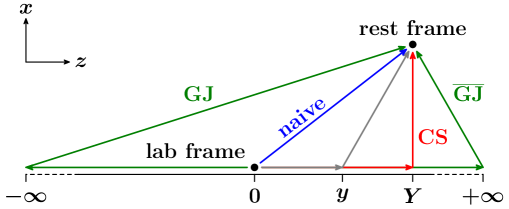
Figure -656: Sequence of boosts definining different vector-boson rest frames. In the general case (gray), we first boost by a rapidity $y$ along the lab-frame beam axis, and then boost into the rest frame. Different choices of $y$ lead to a relative Wigner rotation of the resulting rest frames. Relevant special cases are $y=Y$ (Collins-Soper frame, red), $y=0$ (the naive rest frame, blue) and $y\to\pm\infty$, (Gottfried-Jackson frame, green).

To remove the trivial effect from a mere basis choice at LP, we start from a common LP rest frame at $q_{T}=0$, which is the leptonic frame. A convenient way to parametrize the different possible frames for nonzero $q_{T}$ is by the sequence of boosts starting from the lab frame as shown in figure -656. Specifically, we first boost by a rapidity $y$ along the beam direction and then directly into the rest frame. Some cases of interest are the “naive” rest frame, obtained by performing a single direct boost from the lab frame ($y=0$) into the rest frame, the CS frame ($y=Y$), the Gottfried-Jackson (GJ) frame defined by the limit $y\to-\infty$, or the $\overline{\mathrm{GJ}}$ frame obtained by taking $y\to+\infty$. Another way to conceptualize these frames is through the angles between their respective $z^{\prime\mu}$ axes and the momenta of the incoming protons. In the CS frame, those angles become precisely equal for massless hadrons, see figure -659. In the GJ frame, the $z$ axis is aligned with the direction of $P_{a}$, while the naive case falls in between for $Y>0$.

It is easy to see that for $q_{T}\to 0$, the two boosts for any frame collapse into a single boost from the lab frame to the leptonic frame. Since for $q_{T}\to 0$ all frames coincide, we have

$$r(q)=\mathbf{1}_{3\times 3}+\mathcal{O}(\lambda)\,,\qquad R_{ij}(q)=\delta_{ij}+\mathcal{O}(\lambda)\,.$$ (2.122)

Working at LP in the hadronic tensor, the $\mathcal{O}(\lambda)$ corrections in eq. (2.122) could in principle induce an $\mathcal{O}(\lambda)$ ambiguity in the hadronic power corrections. We now show that this is not the case, which means that the linear power corrections predicted by eq. (2.97) are unique. In other words, we have to show that the absence of additional linear corrections from the hadronic tensor that lead to eq. (2.97) was not just an accident of our particular choice of tensor decomposition.

Eq. (2.122) immediately implies that the new axes still satisfy

$$x^{\prime\mu}=n_{\perp}^{\mu}+\mathcal{O}(\lambda)\,,\qquad y^{\prime\mu}=\epsilon_{\perp}^{\mu\nu}n_{\perp\nu}+\mathcal{O}(\lambda)\,,\qquad z^{\prime\mu}=\frac{n_{a}^{\mu}-n_{b}^{\mu}}{2}+\mathcal{O}(\lambda)\,,$$ (2.123)

so the scaling properties in table 1 also hold for the $W^{\prime}_{j}$. Following our previous analysis, we would now discard all power-suppressed $W^{\prime}_{j}$ structure functions, evaluate the remaining ones ($j=-1,2,4,5$) at leading power, and dress them with exact leptonic tensor components,

$$\frac{\mathrm{d}\sigma^{(0+L)}(\Theta)}{\mathrm{d}^{4}q\,\mathrm{d}\mathcal{O}} =\frac{1}{2E_{\mathrm{cm}}^{2}}\sum_{i}L_{i}(q,\mathcal{O},\Theta)\,\sum_{j=-1,2,4,5}R^{-1}_{ij}(q)\,W^{\prime(0)}_{j}(q^{2},s_{aq},s_{bq})\bigl{[}1+\mathcal{O}(\lambda^{2})\bigr{]}\,.$$ (2.124)

Since all $i=-1,\ldots,7$ are now populated by $R^{-1}_{ij}$, one might think that the different choice of tensor decomposition amounts to a linear power correction compared to the left-hand side as given in eq. (2.102), because the $R_{ij}$ differ from unity by $\mathcal{O}(\lambda)$, but as indicated it is only of $\mathcal{O}(\lambda^{2})$.

To show that the induced difference is indeed only $\mathcal{O}(\lambda^{2})$, first note that rotations around the $z$ axis amount to a trivial shift in $\varphi$. This induces an $\mathcal{O}(\lambda^{2})$ difference at cross-section level due to our assumption of azimuthal symmetry at leading power in eq. (2.88). Hence, it is sufficient to consider the $\mathrm{SO}(2)$ subgroup of rotations around the $y$ axis parametrized by one remaining Euler angle $\alpha$,

$$\begin{pmatrix}x^{\prime\mu}\\ z^{\prime\mu}\\ \end{pmatrix}=\begin{pmatrix}c_{\alpha}&s_{\alpha}\\ -s_{\alpha}&c_{\alpha}\\ \end{pmatrix}\begin{pmatrix}x^{\mu}\\ z^{\mu}\\ \end{pmatrix}\,,\qquad y^{\prime\mu}=y^{\mu}\,,$$ (2.125)

with $c_{\alpha}\equiv\cos\alpha$ and $s_{\alpha}\equiv\sin\alpha$. By a straightforward calculation, the $W_{i}$ can be shown to transform under the following representations of $\mathrm{SO}(2)$:

$$\begin{pmatrix}W^{\prime}_{-1}\\ W^{\prime}_{0}\\ W^{\prime}_{1}\\ W^{\prime}_{2}\\ \end{pmatrix} =\begin{pmatrix}1-\frac{s_{\alpha}^{2}}{2}~{}&\frac{s_{\alpha}^{2}}{2}~{}&-s_{\alpha}c_{\alpha}~{}&\frac{s_{\alpha}^{2}}{4}\\ s_{\alpha}^{2}~{}&1-s_{\alpha}^{2}~{}&2s_{\alpha}c_{\alpha}~{}&-\frac{s_{\alpha}^{2}}{2}\\ s_{\alpha}c_{\alpha}~{}&-s_{\alpha}c_{\alpha}~{}&1-2s_{\alpha}^{2}~{}&-\frac{s_{\alpha}c_{\alpha}}{2}\\ s_{\alpha}^{2}~{}&-s_{\alpha}^{2}~{}&2s_{\alpha}c_{\alpha}~{}&1-\frac{s_{\alpha}^{2}}{2}\end{pmatrix}\begin{pmatrix}W_{-1}\\ W_{0}\\ W_{1}\\ W_{2}\\ \end{pmatrix}\,,$$ (2.126)

$$\begin{pmatrix}W^{\prime}_{3}\\ W^{\prime}_{4}\\ \end{pmatrix} =\begin{pmatrix}c_{\alpha}&s_{\alpha}\\ -s_{\alpha}&c_{\alpha}\\ \end{pmatrix}\begin{pmatrix}W_{3}\\ W_{4}\\ \end{pmatrix}\,,\qquad\begin{pmatrix}W^{\prime}_{5}\\ W^{\prime}_{6}\\ \end{pmatrix}=\begin{pmatrix}c_{\alpha}&s_{\alpha}\\ -s_{\alpha}&c_{\alpha}\\ \end{pmatrix}\begin{pmatrix}W_{5}\\ W_{6}\\ \end{pmatrix}\,,\qquad W^{\prime}_{7}=W_{7}\,.$$

It is a simple exercise in special relativity to show that the resulting Wigner rotation of a generic frame defined by boost $y$ relative to the CS frame with $y=Y$ is

$$\tan\alpha=\frac{\epsilon\sinh(Y-y)\bigl{[}\gamma\cosh(Y-y)-1\bigr{]}}{\gamma\sinh^{2}(Y-y)+\epsilon^{2}\cosh(Y-y)}=\epsilon\tanh\frac{Y-y}{2}+\mathcal{O}(\epsilon^{3})\,,$$ (2.127)

where $\epsilon=q_{T}/Q\sim\lambda$ and $\gamma=\sqrt{1+\epsilon^{2}}$. For any $Y,y$, eq. (2.127) turns out to be bounded by the leading term, $\lvert\tan\alpha\rvert\leq\epsilon\lvert\tanh\frac{Y-y}{2}\rvert\leq\epsilon$. In particular for the GJ frame we have $\tan\alpha_{\mathrm{GJ}}=\epsilon$, with which we recover the well-known result for the relation between $W_{-1,0,1,2}$ in the CS and GJ frames [107].

Eq. (2.127) shows explicitly that $\alpha\sim\lambda$. To see that eq. (2.124) indeed holds up to quadratic power corrections, we invert eq. (2.126) by taking $\alpha\mapsto-\alpha$, and expand in $\alpha\sim\lambda$ to find

$$\begin{pmatrix}W_{-1}\\ W_{0}\\ W_{1}\\ W_{2}\end{pmatrix} =\left[\mathbf{1}_{4\times 4}+\mathcal{O}\begin{pmatrix}\lambda^{2}&\lambda^{2}&\lambda&~{}\lambda^{2}\\ \lambda^{2}&\lambda^{2}&\lambda&~{}\lambda^{2}\\ \lambda&\lambda&\lambda^{2}&~{}\lambda\\ \lambda^{2}&\lambda^{2}&\lambda&~{}\lambda^{2}\\ \end{pmatrix}\right]\begin{pmatrix}W^{\prime}_{\!\!-1}\\ W^{\prime}_{0}\\ W^{\prime}_{1}\\ W^{\prime}_{2}\end{pmatrix}\,,$$

$$\begin{pmatrix}W_{3}\\ W_{4}\end{pmatrix} =\left[\mathbf{1}_{2\times 2}+\mathcal{O}\begin{pmatrix}\lambda^{2}&\lambda\\ \lambda&\lambda^{2}\\ \end{pmatrix}\right]\begin{pmatrix}W^{\prime}_{3}\\ W^{\prime}_{4}\end{pmatrix}\,,$$

$$\begin{pmatrix}W_{5}\\ W_{6}\end{pmatrix} =\left[\mathbf{1}_{2\times 2}+\mathcal{O}\begin{pmatrix}\lambda^{2}&\lambda\\ \lambda&\lambda^{2}\\ \end{pmatrix}\right]\begin{pmatrix}W^{\prime}_{5}\\ W^{\prime}_{6}\end{pmatrix}\,,\quad W_{7}=W^{\prime}_{7}\,.$$ (2.128)

We see that under the rotation, the leading structure functions mix into themselves and into each other only by an $\mathcal{O}(\lambda^{2})$ amount. The subleading structure functions are populated precisely by an amount commensurate with their intrinsic scaling, see table 1. Combined with the scaling of the corresponding leptonic structure functions as in figure -657, we find that the effect of any $\mathcal{O}(\lambda)$ rotation on the cross section is indeed only of $\mathcal{O}(\lambda^{2})$ for LP-azimuthally symmetric observables.

It is natural to ask whether a specific frame choice should be preferred in order to also capture an optimal set of terms at $\mathcal{O}(\lambda^{2})$. It is well known that leading-logarithmic terms are absent in $W_{1}$ in the CS frame [107]. This is natural from the point of view that the CS $z$ axis does not receive power corrections, reducing “spill-over” of terms from the leading-power currents. A reduced size of power corrections by a symmetric choice of frame has also been found for $0$-jettiness $\mathcal{T}_{0}$ [161, 162, 160], albeit for a somewhat different physical reason. In section 4.4 we will find some numerical evidence that the CS decomposition also reduces the size of power corrections in the $\phi^{*}$ spectrum. Taken together, this suggests that the CS frame might indeed be the optimal choice, although the size of the frame-dependent $\mathcal{O}(\lambda^{2})$ corrections should still be assessed.

2.7 Relation to the literature

Early approaches to resummation effects on the Drell-Yan cross section differential in the lepton kinematics [65, 66, 67] typically picked the CS angles to parametrize the decay phase-space integral, but did not discuss the ambiguity inherent in this choice or the relative size of power corrections. In these approaches, the CS frame primarily serves as a tool to enable generic lepton-differential observables. In ref. [107], the logarithmic structure of $W_{-1,0,1,2}$ at low $q_{T}$ in collinear factorization was discussed in detail, but the implications for the structure of power corrections to e.g. the fiducial cross section were not explored.

An implementation of generic lepton-differential observables in $q_{T}$ resummation was presented in ref. [73] and more recently in ref. [74] based on a parton-level Monte-Carlo generation of the leptonic final state. There, the choice of rest frame used in earlier results was recast as a $q_{T}$-recoil prescription for how to distribute the nonzero $q_{T}$ between the colliding partons in the rest frame where the leptonic decay is evaluated. They also showed that the ambiguity in the $q_{T}$-recoil prescription is in one-to-one correspondence with the ambiguity of the rest-frame choice and that it vanishes for $q_{T}\to 0$. They thus argue that the recoil effects are $\mathcal{O}(q_{T}/Q)$ effects that cannot be unambiguously computed through the $q_{T}$ resummation, but some recoil prescription is nevertheless required for practical purposes to satisfy transverse momentum conservation in the parton-level generation of the leptonic decay. (Note that similar recoil prescriptions to preserve momentum conservation are also commonly used in parton-shower Monte Carlos, and in the event-level resummation of ref. [84].)

Very recently, refs. [86, 87] used N³LL perturbative baselines to fit nonperturbative models for the rapidity anomalous dimension and TMDPDFs using fiducial $Z$ $q_{T}$ spectra among other data. They also retain the exact dependence of the fiducial phase space on $q_{T}$, with the analytic leptonic decay matrix element contracted against the LP hadronic tensor $\propto g_{\perp}^{\mu\nu}$ (see also ref. [163]). This is essentially equivalent to an exact treatment of $L_{-1}$ in our notation (up to an overall $\mathcal{O}(\lambda^{2})$ difference in the projection itself), while $L_{4}$ does not contribute to the observables they consider. They also do not provide formal arguments for the exact treatment of the leptonic contributions.

If the fully-differential and flavor-dependent squared leptonic decay matrix element is evaluated and integrated over leptonic phase space accounting for the exact dependence on the vector boson transverse momentum and contracted with the resummed LP hadronic tensor then this amounts to retaining the exact $q_{T}$ dependence of the leptonic tensor. This can be done explicitly at the analytic level or during Monte-Carlo generation via some boost prescription that accounts for the exact $q_{T}$-dependent recoil of the leptonic system. To the best of our understanding this is the case in refs. [73, 74, 84, 86, 87]. Our analysis thus provides formal justification for doing so, showing that the ambiguity inherent in any implementation meeting these criteria is only of $\mathcal{O}(\lambda^{2})$ and that for a large class of common measurements (those that are azimuthally symmetric at LP) this actually unambiguously predicts all linear power corrections along with their resummation for single-boson production. In addition, it is formally required in phase-space regions that exhibit leptonic power corrections.

In ref. [83], fiducial lepton cuts are implemented in the resummed cross section strictly on Born kinematics at $q_{T}=0$, while fiducial power corrections are obtained through the fixed-order matching. Large power corrections from the fixed-order matching were observed in the fiducial case compared to the inclusive case. From our analysis, this is explained by the linear power corrections induced by the fiducial cuts.

Sometimes a multiplicative fixed-order matching procedure is employed, as e.g. in refs. [83, 88], where in order to Sudakov-suppress the fixed-order matching corrections at small $q_{T}$ they are multiplied by the ratio of the LP resummed contribution to its fixed-order expansion. While this procedure is unlikely to produce the correct Sudakov suppression for genuine hadronic power corrections, one might ask if it correctly “dresses” the fiducial power corrections with the LP resummation to achieve their resummation. For this to be the case, the multiplicative matching at minimum has to reproduce eq. (2.97) for the linear power corrections. Clearly, this can only happen if the multiplicative matching only involves a single (effective) hadronic structure function at a time and if it is performed fully differentially in $q^{2}$, $Y$, and $q_{T}^{2}$. This is typically not the case. For example, the multiplicative matching in refs. [83, 88] is performed at the cumulant level, and thus does not satisfy this requirement.

3 Resummation of leading-power hadronic structure functions

In this section, we discuss our specific resummation setup for the leading-power hadronic structure functions $W_{-1,4}^{(0)}$ in eq. (2.103). The setup follows standard procedures and is deliberately kept simple, e.g., by ignoring nonperturbative corrections or quark-mass effects [89] at small $q_{T}$, allowing us to focus on the effect of resumming the fiducial power corrections in the following sections. As discussed in the previous section, the fact that their resummation can be obtained in terms of the leading-power hadronic structure functions, and that this captures all linear as well as leptonic power corrections, holds independently of how precisely the LP resummation is performed.

3.1 Renormalization group evolution

Directly resumming the logarithms of $q_{T}/Q$ in momentum space is challenging due to the vectorial nature of $\vec{q}_{T}$, though by now approaches for doing so exist [76, 77]. As shown in ref. [77], the correct solution of the RGE system in momentum space in terms of distributions is actually equivalent to the canonical solution in conjugate ($b_{T}$) space modulo different boundary conditions. We therefore bypass this issue, as is commonly done, by solving the RGEs in conjugate ($b_{T}$) space. Using that the beam and soft functions only depend on the magnitude $b_{T}=|{\vec{b}}_{T}|$, eq. (2.24b) can be written as

$$[B_{a}B_{b}S](Q^{2},x_{a},x_{b},{\vec{q}}_{T},\mu) =\frac{1}{2\pi}\int_{0}^{\infty}\mathrm{d}b_{T}\,b_{T}J_{0}(b_{T}q_{T})\tilde{B}_{a}(x_{a},b_{T},\mu,\nu/\omega_{a})\,\tilde{B}_{b}(x_{b},b_{T},\mu,\nu/\omega_{b})$$

$$\qquad\qquad\times\tilde{S}(b_{T},\mu,\nu)\,,$$ (3.1)

where $J_{0}(x)$ is the zeroth-order Bessel function of the first kind.

We use the framework of the rapidity renormalization group [62] in conjunction with the exponential regulator of ref. [64], where the beam and soft functions in Fourier space obey the coupled RGEs

$$\frac{\mathrm{d}}{\mathrm{d}\ln\mu}\ln\tilde{B}_{q}(x,b_{T},\mu,\nu/\omega) =\tilde{\gamma}_{B}^{q}(\mu,\nu/\omega)\,,\qquad \frac{\mathrm{d}}{\mathrm{d}\ln\mu}\ln\tilde{S}_{q}(b_{T},\mu,\nu)=\tilde{\gamma}_{S}^{q}(\mu,\nu)\,,$$

$$\frac{\mathrm{d}}{\mathrm{d}\ln\nu}\ln\tilde{B}_{q}(x,b_{T},\mu,\nu/\omega) =-\frac{1}{2}\tilde{\gamma}_{\nu}^{q}(b_{T},\mu)\,,\quad \frac{\mathrm{d}}{\mathrm{d}\ln\nu}\ln\tilde{S}_{q}(b_{T},\mu,\nu)=\tilde{\gamma}_{\nu}^{q}(b_{T},\mu)\,,$$ (3.2)

where the $\mu$ anomalous dimensions on the first line have the all-order expressions

$$\tilde{\gamma}_{B}^{q}(\mu,\nu/\omega) =2\Gamma_{\mathrm{cusp}}^{q}[\alpha_{s}(\mu)]\ln\frac{\nu}{\omega}+\tilde{\gamma}_{B}^{q}[\alpha_{s}(\mu)]\,,$$

$$\tilde{\gamma}_{S}^{q}(\mu,\nu) =4\Gamma_{\mathrm{cusp}}^{q}[\alpha_{s}(\mu)]\ln\frac{\mu}{\nu}+\tilde{\gamma}_{S}^{q}[\alpha_{s}(\mu)]\,.$$ (3.3)

Here, $\Gamma_{\mathrm{cusp}}^{q}(\alpha_{s})$ is the cusp anomalous dimension in the fundamental representation, which is known to four loops [164, 165, 166, 167, 168, 169, 170, 171, 172, 173] (see ref. [171] for a complete list of earlier references). At N³LL we also require the QCD beta function to four loops [174, 175, 176, 177]. The beam and soft noncusp anomalous dimensions $\tilde{\gamma}_{B}^{q}(\alpha_{s})$ and $\tilde{\gamma}_{S}^{q}(\alpha_{s})$ are related to those of the $0$-jettiness beam and soft functions through consistency relations [178] and are known to three loops [179, 180, 131, 181]. The all-order form of the rapidity anomalous dimension $\gamma^{q}_{\nu}$ reads

$$\tilde{\gamma}^{q}_{\nu}(b_{T},\mu) =-4\eta^{q}_{\Gamma}(\mu_{0},\mu)+\tilde{\gamma}^{q}_{\nu,\mathrm{FO}}(b_{T},\mu_{0})\,,\qquad\eta_{\Gamma}^{q}(\mu_{0},\mu)=\int_{\mu_{0}}^{\mu}\!\frac{\mathrm{d}\mu^{\prime}}{\mu^{\prime}}\,\Gamma^{q}_{\rm cusp}[\alpha_{s}(\mu^{\prime})]\,.$$ (3.4)

This form follows from the commutativity of the $\mu$ and $\nu$ derivatives in eq. (3.1). The fixed-order boundary term $\tilde{\gamma}^{q}_{\nu,\mathrm{FO}}$ is known to three loops [131, 134, 182].

The RG evolution factors for $\tilde{B}_{q}$ and $\tilde{S}$ follow by solving the coupled systems of equations in eq. (3.1). One possible way of writing the solution is given by

$$\tilde{B}_{q}\Bigl{(}x,b_{T},\mu,\frac{\nu}{\omega}\Bigr{)} =\tilde{B}_{q}\Bigl{(}x,b_{T},\mu_{B},\frac{\nu_{B}}{\omega}\Bigr{)}\exp\biggl{[}-\frac{1}{2}\ln\frac{\nu}{\nu_{B}}\tilde{\gamma}^{q}_{\nu}(b_{T},\mu_{B})\biggr{]}\exp\biggl{[}\int_{\mu_{B}}^{\mu}\frac{\mathrm{d}\mu^{\prime}}{\mu^{\prime}}\tilde{\gamma}_{B}^{q}(\mu^{\prime},\nu/\omega)\biggr{]}\,,$$

$$\tilde{S}_{q}(b_{T},\mu,\nu) =\tilde{S}_{q}(b_{T},\mu_{S},\nu_{S})\exp\biggl{[}\ln\frac{\nu}{\nu_{S}}\tilde{\gamma}^{q}_{\nu}(b_{T},\mu_{S})\biggr{]}\exp\biggl{[}\int_{\mu_{S}}^{\mu}\frac{\mathrm{d}\mu^{\prime}}{\mu^{\prime}}\tilde{\gamma}_{S}^{q}(\mu^{\prime},\nu)\biggr{]}\,.$$ (3.5)

Here, we evolve first in $\nu$ and then in $\mu$ and the final scale $\mu$ is set to the scale $\mu_{H}$ at which the hard function is evaluated. Any other path in the two-dimensional $(\mu,\nu)$ space connecting $(\mu_{H},\mu_{B},\nu_{B},\mu_{S},\nu_{S})$ is viable as well, and the path independence is ensured by exactly satisfying the RG consistency relations between all anomalous dimensions, in particular by using eq. (3.4). By choosing appropriate boundary scales $\mu_{H,B,S}$ and $\nu_{B,S}$, the hard function, as well as the beam and soft functions on the right-hand side of eq. (3.1) are free of large logarithms and can be evaluated in fixed-order perturbation theory, with all large logarithms resummed through the evolution kernels.

Different methods to numerically evaluate the evolution kernels and integrals over anomalous dimensions entering in eqs. (3.4) and (3.1) were analyzed in detail in ref. [92], which found that their numerical precision becomes relevant at N³LL. Here we use the approximate unexpanded analytic results, which provide sufficient numerical precision for our purposes, with the explicit expressions up to N³LL given in ref. [92]. The anomalous dimensions and fixed-order boundary conditions required for the resummation at N³LL are collected in our notation in refs. [178, 183].

3.2 Canonical scales and nonperturbative prescription

The canonical scales of the hard, beam, and soft functions, and the rapidity anomalous dimension in $b_{T}$ space are given by

$$\mu_{H} \sim Q\,,\qquad \mu_{B} \sim b_{0}/b_{T}\,,\qquad \mu_{S} \sim b_{0}/b_{T}\,,\qquad \mu_{0} \sim b_{0}/b_{T}\,,$$

$$\nu_{B} \sim Q\,,\qquad \nu_{S} \sim b_{0}/b_{T}\,,$$ (3.6)

where $b_{0}\equiv 2e^{-\gamma_{E}}\approx 1.12291$. By evaluating the functions in the factorization theorem at their canonical scales and evolving them to common scales $(\mu,\nu)$, all logarithms of $\mu_{B}/\mu_{H}\sim\mu_{S}/\mu_{H}\sim\nu_{S}/\nu_{B}\sim(b_{0}/b_{T})/Q$ are resummed. In ref. [77] it was shown that the resummation in $b_{T}$ space with the canonical scales in eq. (3.2) is in fact equivalent to the exact solution of the RGE in momentum space, i.e., it reproduces the canonical, distributional logarithms in $q_{T}$, except for the fact that one effectively uses a shifted set of finite terms in the boundary conditions (similar to the difference between renormalization schemes). We exploit this and require that for $q_{T}\ll Q$, eq. (3.2) is exactly satisfied, such that the resummed $q_{T}$ spectrum in this region is obtained from the numerical inverse Fourier transform of the canonical $b_{T}$-space result.

With the choice in eq. (3.2), the beam and soft functions and the rapidity anomalous dimension become sensitive to nonperturbative effects at large $b_{T}\gtrsim\Lambda_{\mathrm{QCD}}^{-1}$. The Landau pole can be avoided by choosing $\mu_{0}$ (and $\mu_{B},\mu_{S}$) as a function of $b_{T}$ such that it asymptotes to a perturbative value at large $b_{T}$, see e.g. ref. [80] for a concrete implementation. Alternatively, a global replacement of $b_{T}$ by a suitable function $b^{*}(b_{T})$ may be performed at the level of the cross section, where $b^{*}(b_{T})$ itself is bounded by some perturbative value $b_{\mathrm{max}}\lesssim 1/\Lambda_{\mathrm{QCD}}$ [56, 57]. In either case, the mismatch to the full result is then in principle captured by a corresponding nonperturbative contribution. Recently, it was shown that the full $\tilde{\gamma}^{i}_{\nu}$ may also be determined from lattice calculations [184, 185, 186, 187, 188], and that estimates of the first subleading power in $b_{T}\Lambda_{\mathrm{QCD}}$ can also be related to the gluon condensate [189].

Since nonperturbative effects in the region $q_{T}\sim\Lambda_{\mathrm{QCD}}$ are not the main focus of this work, we use a simpler prescription to ensure that $\alpha_{s}$ remains perturbative. Specifically, we freeze out both the running coupling and the PDFs entering the hadronic structure functions $W_{-1,4}^{(0)}$ at a perturbative scale by performing the replacement

$$\alpha_{s}(\mu)\mapsto\alpha_{s}^{\mathrm{fr}}(\mu)\equiv\alpha_{s}\bigl{[}\mu_{\mathrm{fr}}(\mu)\bigr{]}\,,\qquad f_{i}(\mu)\mapsto f_{i}^{\mathrm{fr}}(\mu)\equiv f_{i}[\mu_{\mathrm{fr}}(\mu)\bigr{]}\,.$$ (3.7)

We choose the smooth function $\mu_{\mathrm{fr}}(\mu)$ governing the freeze-out as

$$\mu_{\mathrm{fr}}(\mu)=\begin{cases}\Lambda_{\mathrm{fr}}+\frac{\mu^{2}}{4\Lambda_{\mathrm{fr}}}&\mu\leq 2\Lambda_{\mathrm{fr}}\,,\\ \mu&\mu>2\Lambda_{\mathrm{fr}}\,.\end{cases}$$ (3.8)

In practice, we pick $\Lambda_{\mathrm{fr}}=1\,\mathrm{GeV}$ for our central results. The behavior of $\alpha_{s}^{\mathrm{fr}}$ at low scales is illustrated in the left panel of figure -655. This choice constitutes a (fairly crude) model for the large $b_{T}$ behavior of $\tilde{\gamma}_{\nu}^{i}$ that is sufficient to regulate the large $b_{T}$ region, and formally amounts to a power correction in $\Lambda_{\mathrm{QCD}}\ll q_{T}$. We similarly ignore contributions of $\mathcal{O}(b_{T}\Lambda_{\mathrm{QCD}})$ in the beam and soft function boundary conditions, beyond the ones encoded in our global choice of $\mu_{\mathrm{fr}}(\mu)$. This is also consistent with neglecting the hadronic structure functions $W_{2,5}$ involving Boer-Mulders functions in the regime $\Lambda_{\mathrm{QCD}}\ll q_{T}\ll Q$ altogether, see the discussion below eq. (2.103). We have checked that for perturbative $q_{T}\gtrsim 2\,\mathrm{GeV}$, the results from our prescription are compatible with a traditional (global) $b^{\ast}$ prescription [56, 57] within the uncertainty estimated by varying $\Lambda_{\mathrm{fr}}$ as described in section 3.4.

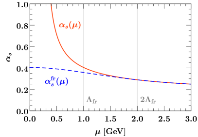
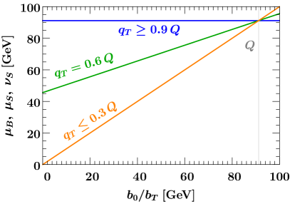
Figure -655: Left: Illustration of the freeze-out prescription used to ensure that $\alpha_{s}$ is evaluated at perturbative scales. Right: Hybrid profile scales as a function of $b_{0}/b_{T}$ for representative values of $q_{T}$. The thin vertical line corresponds to $b_{0}/b_{T}=Q$, where $Q=m_{Z}$ for illustration purposes.

3.3 Fixed-order matching and profile scales

We extend the description of the cross section to the fixed-order region $q_{T}\sim Q$ by an additive matching to the fixed-order result via profile scales,

$$\mathrm{d}\sigma=\mathrm{d}\sigma^{(0+L)}(\mu_{\mathrm{res}})+\bigl{[}\mathrm{d}\sigma^{\mathrm{FO}}(\mu_{\mathrm{FO}})-\mathrm{d}\sigma^{(0+L)}(\mu_{\mathrm{FO}})\bigr{]}\,.$$ (3.9)

Here the $\mu_{\mathrm{res}}$ argument of the first term indicates that we evaluate the resummed LP hadronic structure functions in $\mathrm{d}\sigma^{(0+L)}$ using the resummation profile scales given below. The argument $\mu_{\mathrm{FO}}$ in the last term indicates that they are instead evaluated at common fixed-order scales $\mu_{\mathrm{FO}}$, which can be done directly in momentum space. The last term effectively acts as a differential subtraction term for the full fixed-order cross section $\mathrm{d}\sigma^{\mathrm{FO}}$ in the second term, such that the difference in square brackets is a nonsingular power correction. We will refer to the outcome of eq. (3.9) as N³LL${}^{(0+L)}+$NNLO₀ when the resummed LP hadronic structure functions at N³LL are combined with the exact leptonic tensor as discussed in section 2.5, and matched to the fixed $\mathcal{O}(\alpha_{s}^{2})$ NNLL₀ result. When instead evaluating the leptonic tensor at strict LP, we refer to it as N³LL${}^{(0)}+$NNLO₀, in which case the fiducial power corrections are only included through the fixed-order matching. The analogous notation is used at lower orders.

Approaching $q_{T}\sim Q$, the $q_{T}$ resummation must be turned off to ensure the delicate cancellations between singular and nonsingular contributions and to properly recover the correct fixed-order result for the spectrum, i.e., such that the difference between the first and last terms in eq. (3.9) smoothly vanishes for $q_{T}\sim Q$. To achieve this, we use the method of profile scales [190, 191]. We use the hybrid profile scales constructed in ref. [80], which depend on both $b_{T}$ and $q_{T}$, and undergo a continuous deformation away from the canonical $b_{T}$ scales in eq. (3.2) as a function of the target $q_{T}$ value, schematically,

$$\mu_{B,S}(q_{T},b_{T})\,,\nu_{B,S}(q_{T},b_{T})\to\mu_{H}=\mu_{\mathrm{FO}}\quad\text{for}\quad q_{T}\to Q\,.$$ (3.10)

We note that $\mu_{0}$ does not need to asymptote to $\mu_{\mathrm{FO}}$ towards large $q_{T}$ because its effect on the matched result is already turned off as $\nu_{S}\to\nu_{B}$. In this limit, the first and last term in eq. (3.9) exactly cancel, leaving the fixed-order result $\mathrm{d}\sigma^{\mathrm{FO}}$. We choose central scales as

$$\mu_{H}=\nu_{B}=\mu_{\mathrm{FO}}\,,\qquad\mu_{B}=\mu_{S}=\nu_{S}=\mu_{\mathrm{FO}}\,f_{\mathrm{run}}\Bigl{(}\frac{q_{T}}{Q},\frac{b_{0}}{b_{T}\,Q}\Bigr{)}\,,\qquad\mu_{0}=\frac{b_{0}}{b_{T}}\,,$$ (3.11)

where $f_{\mathrm{run}}$ is a hybrid profile function given by

$$f_{\mathrm{run}}(x,y) =1+g_{\mathrm{run}}(x)(y-1)\,.$$ (3.12)

It controls the amount of resummation by adjusting the slope of the scales in $b_{T}$ space as a function of $q_{T}/Q$ via the function

$$g_{\mathrm{run}}(x) =\begin{cases}1&0<x\leq x_{1}\,,\\ 1-\frac{(x-x_{1})^{2}}{(x_{2}-x_{1})(x_{3}-x_{1})}&x_{1}<x\leq x_{2}\,,\\ \frac{(x-x_{3})^{2}}{(x_{3}-x_{1})(x_{3}-x_{2})}&x_{2}<x\leq x_{3}\,,\\ 0&x_{3}\leq x\,.\end{cases}$$ (3.13)

As a result, for $q_{T}\leq x_{1}Q$, the slope is unity yielding the canonical resummation, while for $q_{T}\geq x_{3}Q$, the slope vanishes so the resummation is fully turned off. In between, the slope smoothly transitions from one to zero, which transitions the resummation from being canonical to being turned off. This is illustrated in the right panel of figure -655. Note that in contrast to ref. [80], we do not require a deformation away from the canonical scales to regulate the Landau pole at large $b_{T}$, but instead rely on the replacement in eq. (3.7). For our central results, we use the transition points $(x_{1},x_{2},x_{3})=(0.3,0.6,0.9)$.

3.4 Estimate of perturbative uncertainties

We identify several sources of perturbative uncertainties, which we estimate as follows. In the limit $q_{T}\ll Q$, the perturbative uncertainty is driven by the combined uncertainty from truncating the expansion of the soft, beam, and rapidity anomalous dimensions. To estimate them, we adopt the set of SCET_II profile scale variations introduced in ref. [192] for a SCET_II-like jet veto. They are given by

$$\mu_{S} =\mu_{\mathrm{FO}}\,\Bigl{[}f_{\mathrm{vary}}\Bigl{(}\frac{q_{T}}{Q}\Bigr{)}\Bigr{]}^{v_{\mu_{S}}}\,f_{\mathrm{run}}\Bigl{(}\frac{q_{T}}{Q},\frac{b_{0}}{b_{T}Q}\Bigr{)}\,,$$

$$\nu_{S} =\mu_{\mathrm{FO}}\,\Bigl{[}f_{\mathrm{vary}}\Bigl{(}\frac{q_{T}}{Q}\Bigr{)}\Bigr{]}^{v_{\nu_{S}}}\,f_{\mathrm{run}}\Bigl{(}\frac{q_{T}}{Q},\frac{b_{0}}{b_{T}Q}\Bigr{)}\,,$$

$$\mu_{B} =\mu_{\mathrm{FO}}\,\Bigl{[}f_{\mathrm{vary}}\Bigl{(}\frac{q_{T}}{Q}\Bigr{)}\Bigr{]}^{v_{\mu_{B}}}\,f_{\mathrm{run}}\Bigl{(}\frac{q_{T}}{Q},\frac{b_{0}}{b_{T}Q}\Bigr{)}\,,$$

$$\nu_{B} =\mu_{\mathrm{FO}}\,\Bigl{[}f_{\mathrm{vary}}\Bigl{(}\frac{q_{T}}{Q}\Bigr{)}\Bigr{]}^{v_{\nu_{B}}}\,,$$ (3.14)

where each of the four variation exponents can be $v_{i}=\{+1,0,-1\}$, and the amount of variation is governed by

$$f_{\mathrm{vary}}(x)=\begin{cases}2(1-x^{2}/x_{3}^{2})&0\leq x<x_{3}/2\,,\\ 1+2(1-x/x_{3})^{2}&x_{3}/2\leq x<x_{3}\,,\\ 1&x_{3}\leq x\,,\end{cases}$$ (3.15)

i.e., as $q_{T}\to Q$, this source of perturbative uncertainty is turned off together with the resummation as a whole. The central scale choice corresponds to $(v_{\mu_{S}},v_{\nu_{S}},v_{\mu_{B}},v_{\nu_{B}})=(0,0,0,0)$, and a priori there are 80 possible different combinations of the $v_{i}$. Since the arguments of the resummed logarithms are ratios of scales, some combinations of scale variations will lead to variations of these arguments that are larger than a factor of two, and are therefore excluded. After dropping these combinations we are left with 36 different scale variations. By taking their maximum envelope, we obtain an estimate of the resummation uncertainty $\Delta_{\mathrm{res}}$. Note that independent variations of $\mu_{H}$ need not be considered as part of $\Delta_{\mathrm{res}}$ because the corresponding change in the argument of the resummed logarithms is already covered by eq. (3.4).

Second, we estimate the fixed-order perturbative uncertainty $\Delta_{\mathrm{FO}}$ from the maximum envelope of overall variations of $\mu_{\mathrm{FO}}$ by a factor of two. These variations are inherited by all the resummation scales in eq. (3.11), so they leave the resummed logarithms invariant. Third, we estimate the inherent uncertainty $\Delta_{\mathrm{match}}$ in our matching procedure eq. (3.9) by taking the maximum envelope of explicit variations of the transition points $x_{i}$,

$$(x_{1},x_{2},x_{3})=\bigl{\{}(0.4,0.75,1.1),\,(0.2,0.45,0.7),\,(0.4,0.55,0.7),\,(0.2,0.65,1.1)\bigr{\}}\,.$$ (3.16)

Finally, we consider two independent variations of $\Lambda_{\mathrm{fr}}=\{0.8,1.5\}\,\mathrm{GeV}$ away from our central choice $\Lambda_{\mathrm{fr}}=1\,\mathrm{GeV}$ as a rough estimate of the uncertainty $\Delta_{\Lambda}$ in our nonperturbative prescription. Combining all sources of uncertainty in quadrature, we take

$$\Delta_{\mathrm{total}}=\sqrt{\Delta_{\mathrm{res}}^{2}+\Delta_{\mathrm{FO}}^{2}+\Delta_{\mathrm{match}}^{2}+\Delta_{\Lambda}^{2}}$$ (3.17)

as an estimate of the total (perturbative) uncertainty on our results.

4 Resumming fiducial power corrections

As discussed in section 2.5, fiducial power corrections arise entirely from the leptonic tensors $L_{i}(q,\mathcal{O},\Theta)$, and accordingly can be treated exactly in the factorization by keeping the $L_{i}$ exact. In this section, we consider three applications to discuss this mechanism in more detail, namely the $q_{T}$ spectrum with fiducial cuts (section 4.2), the lepton transverse momentum distribution ($p_{T}^{\ell}$) (section 4.3), and the $\phi^{*}$ observable (section 4.4). In all cases, we consider our primary examples of $Z\to\ell^{+}\ell^{-}$ or $W\to\ell\nu$.

4.1 Numerical inputs and computational setup

All our numerical results in this and the following sections are obtained using the following setup. We use the CT18NNLO [193] PDF set, and correspondingly use the three-loop running to obtain the numerical value of $\alpha_{s}$ at any required scale with $\alpha_{s}(91.1870)=0.118$ as starting point. We use the same PDF also at lower orders, which is consistent and allows us to exhibit the genuine size of perturbative corrections.

For the resonant $W$ and $Z$ propagators, we work in the fixed-width pole scheme. We use the following electroweak parameters [194]

$$m_{Z} =91.1535\,\mathrm{GeV}\,,\qquad\,\,\Gamma_{Z}=2.4943\,\mathrm{GeV}\,,$$

$$m_{W} =80.3580\,\mathrm{GeV}\,,\qquad\Gamma_{W}=2.0843\,\mathrm{GeV}\,,$$ (4.1)

$$G_{F} =1.1663787\times 10^{-5}\,\mathrm{GeV}^{-2}\,,$$

$$V_{\rm CKM} =\begin{pmatrix}V_{ud}\quad V_{us}\quad V_{ub}\\ V_{cd}\quad V_{cs}\quad V_{cb}\\ V_{td}\quad V_{ts}\quad V_{tb}\\ \end{pmatrix}=\begin{pmatrix}0.97446\quad 0.22452\quad 0.00365\\ 0.22438\quad 0.97359\quad 0.04214\\ ~{}0.00896\quad 0.04133\quad 0.999105\\ \end{pmatrix}\,.$$ (4.2)

For the electroweak couplings, we use the $G_{\mu}$ scheme, with the values for $\alpha_{\mathrm{em}}$ and $\sin^{2}\theta_{w}$ obtained from $m_{W}$, $m_{Z}$, and $G_{F}$ as

$$\sin^{2}\theta_{w} =1-\frac{m_{W}^{2}}{m_{Z}^{2}}=0.22284\,,$$

$$\alpha_{\mathrm{em}}\equiv\alpha_{\mu} =\frac{\sqrt{2}G_{F}}{\pi}\,m_{W}^{2}\Bigl{(}1-\frac{m_{W}^{2}}{m_{Z}^{2}}\Bigr{)}=\frac{1}{132.357}\,.$$ (4.3)

All factorized cross sections, both at fixed order and including resummation up to N³LL accuracy as described in section 3 are obtained from the C++ library SCETlib [114]. By default we use the CS tensor decomposition, and LP cross sections including fiducial power corrections are denoted as $\sigma^{(0+L)}$, while those at strict LP without fiducial power corrections are denoted by $\sigma^{(0)}$. We have also implemented alternative tensor decompositions using eq. (2.124), in particular the one that corresponds to the GJ frame, and will denote cross sections evaluated using this choice as $\sigma^{(0+L)}_{\mathrm{GJ}}$. SCETlib uses the Cuba 4.2 library [195, 196] for adaptive multi-dimensional integration over $Q$ and $Y$, combined with $q_{T}$ integrals whenever they cannot be performed analytically. To perform oscillatory Bessel integrals for inverse Fourier transforms we use a double-exponential method for oscillatory integrals [197, 198, 199].

The integral over the leptonic phase space appearing in eq. (2.60),

$$\int_{-1}^{1}\!\mathrm{d}\cos\theta\,\int_{0}^{2\pi}\mathrm{d}\varphi\,g_{i}(\theta,\varphi)\,\delta[\mathcal{O}-\hat{\mathcal{O}}(q,\theta,\varphi)]\,\hat{\Theta}(q,\theta,\varphi)\,,$$ (4.4)

is carried out semi-analytically as follows. We focus on binned observables $\hat{\Theta}(q,\theta,\varphi)$ and assume that the differential measurement $\mathcal{O}$ on the decay products is being integrated over. We assume that the measurement cuts and bins $\hat{\Theta}(q,\theta,\varphi)$ evaluate to $1$ when all cuts are passed and $0$ otherwise, i.e., we take it to be a product of $\theta$ functions. An explicit dependence on $\theta$ or $\varphi$, e.g. to apply angular projections, can also easily be accommodated, but this is not needed for the results obtained in this paper. For given values of $q$ and $\varphi$, we first determine all intervals in $\cos\theta$ that pass the given cuts. Notably, for all observables considered here ($p_{T1,2}$, $\eta_{1,2}$, $\phi^{*}$, and any of their combinations), the interval boundaries can be evaluated analytically even for nonzero $q_{T}$. The integral over $\cos\theta$ over these intervals is then carried out analytically. The remaining integral over $\varphi$ is performed by adaptive numerical integration. In practice, the sum over hadronic structure functions $i$, see eq. (2.102), can be pulled under the integral in eq. (4.4) because the structure functions only depend on the given value of $q$, so the decay phase-space boundaries only have to be determined once. Typical evaluation times even for complicated phase-space volumes are in the few-millisecond range on a single Intel^® Core™ i5-7200U CPU @ $2.50\,\mathrm{GHz}$ for a target relative numerical precision of $10^{-7}$. The algorithm is not restricted to the leading-power structure functions, but can also be used standalone with generic hadronic structure functions that are provided.

Fixed-order results for $q_{T}$ and $\phi^{*}$ at LO₁ and NLO₁ for the relevant Born$+1$-parton cross sections are obtained from MCFMv8 [200, 201, 202]. These results are used in the fixed-order matching. In addition, they are used to obtain $q_{T}$ (or $\phi^{*}$) integrated cross sections at NLO₀ and NNLO₀ by combining them with $q_{T}$ (or $\phi^{*}$) subtractions including fiducial power corrections supplied by SCETlib. This setup is discussed in more detail in section 5. We stress that the inclusion of fiducial power corrections in the subtractions is essential to obtain numerically stable results down to very small $q_{T}$ and $\phi^{*}$ and for $p_{T}^{\ell}$ near the Jacobian peak.

4.2 $q_{T}$ spectrum with fiducial cuts

We first discuss the impact of fiducial cuts on the Drell-Yan $q_{T}$ spectrum. We consider the standard kinematic selection cuts of requiring a minimum transverse momentum $p_{T}^{\mathrm{min}}$ and maximum rapidity $\eta_{\mathrm{max}}$ of the final-state leptons,

$$\Theta:\qquad p_{T,i}\geq p_{T}^{\mathrm{min}}\,,\quad|\eta_{i}|\leq\eta_{\mathrm{max}}\,,$$ (4.5)

where $p_{T,i}$ and $\eta_{i}$ with $i=1,2$ are the transverse momentum and pseudorapidity of the two leptons.

4.2.1 Origin of power corrections

The $p_{T}^{\mathrm{min}}$ cut was already discussed in detail in ref. [104]. Here, we briefly review the key steps and results, and in addition discuss the rapidity cut. A useful parametrization of the total momentum $q^{\mu}$ and the lepton momenta $p_{1,2}^{\mu}$ in the lab frame is

$$q^{\mu} =\bigl{(}m_{T}\cosh Y\,,\,q_{T},\,0\,,m_{T}\sinh Y\bigr{)}\,,$$

$$p_{1}^{\mu} =p_{T,1}\bigl{(}\cosh(Y+{\Delta y})\,,\,\cos\psi\,,\,\sin\psi\,,\,\sinh(Y+{\Delta y})\bigr{)}\,,$$

$$p_{2}^{\mu} =q^{\mu}-p_{1}^{\mu}\,,$$ (4.6)

where $m_{T}=(Q^{2}+q_{T}^{2})^{1/2}$. As before, we neglect the lepton masses and align the total transverse momentum ${\vec{q}}_{T}$ with the $x$-axis. We denote the azimuthal angle of the first lepton in the lab frame as $\psi$ to distinguish it from the CS angle $\varphi$, and write its rapidity as $y_{1}=Y+{\Delta y}$. Momentum conservation determines $p_{2}^{\mu}$, and fixes the transverse momenta and rapidities of the leptons to

$$p_{T,1} =\frac{Q^{2}/2}{m_{T}\cosh({\Delta y})-q_{T}\cos\psi}\,,\quad \eta_{1}=Y+{\Delta y}\,,$$

$$p_{T,2} =\sqrt{p_{T,1}^{2}-2q_{T}\,p_{T,1}\cos\psi+q_{T}^{2}}\,,\quad \eta_{2}=Y+\frac{1}{2}\ln\frac{m_{T}-p_{T,1}e^{+{\Delta y}}}{m_{T}-p_{T,1}e^{-{\Delta y}}}\,.$$ (4.7)

For compactness, here we do not substitute $p_{T,1}$ in the expressions for $p_{T,2}$ and $\eta_{2}$. The two-particle phase space defined in eq. (2.10) then takes the form

$$\mathrm{d}\Phi_{L}(q) =\frac{p_{T,1}^{2}}{8\pi^{2}Q^{2}}\,\mathrm{d}\psi\,\mathrm{d}{\Delta y}\,.$$ (4.8)

The integrated phase space with the cuts in eq. (4.5) can now be written as

$$\Phi_{L}(q,p_{T}^{\mathrm{min}},\eta_{\mathrm{max}}) =\int\!\mathrm{d}\Phi_{L}(q)\,\theta\bigl{(}p_{T,1}\geq p_{T}^{\mathrm{min}}\bigr{)}\theta\bigl{(}p_{T,2}\geq p_{T}^{\mathrm{min}}\bigr{)}\theta\bigl{(}|\eta_{1}|\leq\eta_{\mathrm{max}})\theta\bigl{(}|\eta_{2}|\leq\eta_{\mathrm{max}})$$

$$=\int_{0}^{2\pi}\mathrm{d}\psi\int_{-\infty}^{\infty}\mathrm{d}{\Delta y}\,\frac{p_{T,1}^{2}}{8\pi^{2}Q^{2}}\,$$

$$\qquad\times\theta\bigl{(}\min\{p_{T,1},p_{T,2}\}\geq p_{T}^{\mathrm{min}}\bigr{)}\,\theta\bigl{(}\max\{|\eta_{1}|,|\eta_{2}|\}\leq\eta_{\mathrm{max}}\bigr{)}\,.$$ (4.9)

The integrand in eq. (4.2.1) depends on $q_{T}$ only through the combinations $q_{T}^{2}$ and $q_{T}\cos\psi$. Thus, the expansion of the integrand in the limit $q_{T}\ll Q$ can only yield linear fiducial corrections if the $\psi$ integral does not average out. This is equivalent to requiring that the cuts break azimuthal symmetry, as otherwise the $\psi$ integral can always be trivially carried out, such that all odd powers of $q_{T}\cos\psi$ integrate to zero and only quadratic corrections in $(q_{T}/Q)^{2}$ arise. Inclusive measurements are a special case, as without cuts $\Phi_{L}(q)$ can only depend on $q^{2}$.

To see this mechanism explicitly for cuts on $p_{T}$ and $\eta$, we expand the lepton transverse momenta and rapidities in eq. (4.2.1) in $q_{T}/Q\sim\lambda$,

$$p_{T,1} =\frac{Q}{2\cosh{\Delta y}}\biggl{[}1+\frac{q_{T}}{Q}\frac{\cos\psi}{\cosh{\Delta y}}+\mathcal{O}(q_{T}^{2}/Q^{2})\biggr{]}\,,$$

$$p_{T,2} =p_{T,1}-q_{T}\cos\psi+\mathcal{O}(q_{T}^{2}/Q^{2})\,,$$

$$\eta_{1} =Y+{\Delta y}\,,$$

$$\eta_{2} =Y-{\Delta y}-2\frac{q_{T}}{Q}\cos\psi\sinh{\Delta y}+\mathcal{O}(q_{T}^{2}/Q^{2})\,.$$ (4.10)

All observables in eq. (4.2.1) have a well-defined, nonvanishing LP limit as $q_{T}\to 0$, and the first correction is proportional to $q_{T}\cos\psi$. Since at $q_{T}=0$, $\psi$ and $\varphi$ coincide, we immediately find that the fiducial $q_{T}$ spectrum obeys azimuthal symmetry at leading power, so the discussion in section 2.5.1 applies.

Naively, one might also expect that all linear fiducial corrections vanish upon integration over $\psi$. However, this is spoiled by the minimum and maximum in the $\theta$ functions in eq. (4.2.1), as can be easily seen for the $p_{T}^{\mathrm{min}}$ cut. For $\cos\psi>0$, one has $p_{T,1}>p_{T,2}$, and thus the $\theta$ function in eq. (4.2.1) only restricts $p_{T,2}$. Vice versa, for $\cos\psi<0$ it is $p_{T,1}$ that is constrained. This leads to two different integrands of the $\psi$ integral in the two integration regions, leading to a nonvanishing $\psi$ integral. This shows that the azimuthal symmetry is explicitly broken at $\mathcal{O}(\lambda)$ leading to linear fiducial power corrections. However, it also shows that if one were to only apply cuts to one of the leptons while being fully inclusive in the other, no linear power corrections from the cuts would arise, since the $\psi$ integral would average out when integrated against the $g_{-1,2,4,5}(\theta,\varphi)$ (using again that the difference between $\psi$ and $\varphi$ is itself of order $q_{T}$).

The situation is more complicated for the rapidity cut. Determining the transition point of the maximum in the corresponding $\theta$ function in eq. (4.2.1), i.e. the value $\psi_{\mathrm{tp}}$ for which $|\eta_{1}|=|\eta_{2}|$, we find that

$$\cos\psi_{\mathrm{tp}}=\frac{Q}{2q_{T}}\frac{\sinh(2Y)}{\sinh(2Y+{\Delta y})}\times\bigl{[}1+\mathcal{O}(q_{T}^{2}/Q^{2})\bigr{]}\,.$$ (4.11)

If $\lvert\cos\psi_{\mathrm{tp}}\rvert\geq 1$, then the $\theta$ function in eq. (4.2.1) only restricts either $|\eta_{1}|$ or $|\eta_{2}|$ but not both for the whole $\psi$ range. In this case, the rapidity cut does not break azimuthal symmetry.

For small but nonvanishing values of $q_{T}$, the $Q/q_{T}$ scaling in eq. (4.11) can be overcome by a sufficiently small value of the vector-boson rapidity $Y$. To be precise, eq. (4.11) has a solution in the physical range $\lvert\cos\psi_{\mathrm{tp}}\rvert<1$ when

$$q_{T}>\frac{Q}{2}\biggl{|}\frac{\sinh(2Y)}{\sinh(2Y+{\Delta y})}\biggr{|}\,.$$ (4.12)

Note that the $\eta_{1}$ constraint always requires that $|Y+{\Delta y}|\leq\eta_{\mathrm{max}}$. Furthermore, we are only interested in the $q_{T}\ll Q$ limit, which implies that eq. (4.12) only becomes important when $|Y|\ll 1$. Hence, linear fiducial corrections will only arise in the region

$$\frac{q_{T}}{Q}\gtrsim\frac{q_{T}^{\mathrm{tp}}}{Q}\equiv\frac{|Y|}{\sinh(\eta_{\mathrm{max}})}\,,\qquad|Y|\ll 1\,,$$ (4.13)

while for $q_{T}\lesssim q_{T}^{\mathrm{tp}}$ only quadratic power corrections arise. Note that in the region $q_{T}\sim q_{T}^{\mathrm{tp}}\ll Q$ the standard power counting breaks down, as one has to simultaneously expand $|Y|\sim q_{T}/Q\ll 1$. This is an example of a leptonic fiducial power correction as discussed in section 2.5.2, where it is crucial to keep the lepton phase space exact to correctly account for both small scales $q_{T}/Q$ and $|Y|$. In practice, the size of this region is of $\mathcal{O}(|Y|)$ and thus small by construction, and hence its contribution to the cross section when integrated over or binned in $Y$ is suppressed as well.

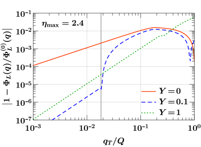
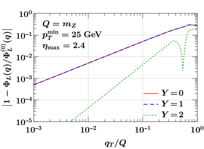
Figure -654: Relative difference of the exact dilepton phase space with fiducial cuts to its LP (Born) limit, for various values of the total dilepton rapidity $Y$ for a pure rapidity cut (left) and both rapidity and $p_{T}$ cuts (right). The thick vertical line on the left shows transition point in eq. (4.12) for $Y=0.1$.

To illustrate and validate our observations, we have numerically implemented the exact phase space with cuts in eq. (4.2.1). In figure -654, we show the relative difference of the dilepton phase space as a function of $q_{T}/Q$ for the cut $\eta_{\mathrm{max}}=2.4$ (left) and the combined cut $p_{T}^{\mathrm{min}}=25~{}\,\mathrm{GeV}$ and $\eta_{\mathrm{max}}=2.4$ (right), for different values of the total rapidity $Y$ and fixed $Q=m_{Z}$. In the left plot, one can clearly see that for $Y=0$ one has a linear power correction for small $q_{T}$ up to $q_{T}/Q\sim 0.1$ (red solid line). For the slightly larger value $Y=0.1$ (blue dashed line), we observe quadratic corrections up to the transition point $q_{T}^{\mathrm{tp}}/Q\approx 0.2$, indicated by the thick vertical line, while above this transition the correction has no simple scaling behavior. Finally, for the relatively large value $Y=1$ one has quadratic corrections essentially throughout the whole $q_{T}$ spectrum (green dotted line). Also note that, in general, the corrections to the phase space are rather small, as even for $Y=0.1$ they do not exceed $1\%$ for $q_{T}/Q<0.1$.

In the right plot in figure -654, we apply both $\eta_{\mathrm{max}}$ and $p_{T}^{\mathrm{min}}$ cuts. For small values of $Y$, the $p_{T}^{\mathrm{min}}$ cut is a stronger constraint on the phase space than the $\eta_{\mathrm{max}}$ cut. Hence, the two curves for $Y=0$ (red solid) and $Y=1$ (blue dashed) are equal, as the $p_{T}^{\mathrm{min}}$ constraint is independent of rapidity. For large $Y\sim\eta_{\mathrm{max}}$, the rapidity cut dominates over the $p_{T}$ cut, as illustrated for $Y=2$ (green dotted), and one only has quadratic power corrections.

4.2.2 Numerical results

Having explicitly demonstrated that linear power corrections to the $q_{T}$ spectrum arise from fiducial cuts on the final-state leptons, we now verify that they can indeed be captured in the factorization theorem by keeping the lepton kinematics exact, as discussed in section 2.5.1. In the following, we will always consider the fiducial cut

$$p_{T}^{\ell}\geq 25~{}\,\mathrm{GeV}\,,\quad|\eta_{\ell}|\leq 2.4\,,$$ (4.14)

as employed in the CMS Drell-Yan measurement at 13 TeV [15].

In figure -653, we show the $q_{T}$ spectrum for $Q=m_{Z}$ at NLO₀, both without (left) and with (right) fiducial cuts. In both figures, the red points illustrate the full NLO₀ result, while the solid blue line shows the result at $\sigma^{(0)}$ (left) and at $\sigma^{(0+L)}$ (right). The various dotted and dashed lines show the differences between the full result and different singular limits. In the inclusive case (left panel), there are no linear power corrections, and thus $\sigma-\sigma^{(0)}$ (green, dashed) scales quadratically in $q_{T}$, as expected. With fiducial cuts (right panel), $\sigma-\sigma^{(0)}$ (gray, dotted) clearly suffers from linear power corrections, and as explained before, these linear corrections can be accounted for by keeping the leptonic tensor exact. This is illustrated by the green-dashed line, which shows the difference $\sigma-\sigma^{(0+L)}$ between the exact and NLP result, and only depends quadratically on $q_{T}$. In particular, the size of these corrections is comparable to the quadratic corrections in the inclusive case. The orange, dot-dashed curve shows the difference $\sigma^{(0+L)}_{\rm GJ}-\sigma^{(0+L)}$ between two choices of the tensor decomposition, corresponding to the CS frame and the GJ frame. This difference scales quadratically in $q_{T}$, confirming that the ambiguity from the choice of tensor decomposition is quadratically suppressed. Moreover, we observe that this ambiguity is numerically much smaller than $\sigma^{(0+L)}$ itself, indicating that it may be completely negligible in practice.

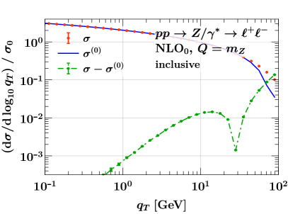
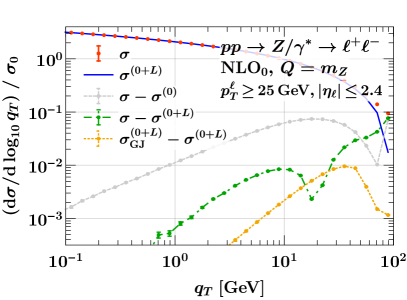
Figure -653: Power corrections for the $q_{T}$ spectrum in Drell-Yan production, inclusive in the decay products (left) and with fiducial cuts (right).

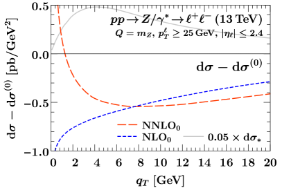
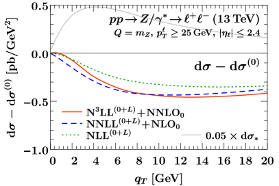
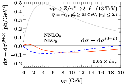
Figure -652: Breakdown of subleading-power contributions to the fiducial Drell-Yan $q_{T}$ on the resonance, $Q=m_{Z}$. We compare the sum of all subleading power contributions, treating the linear fiducial power corrections at fixed order (top left) or resumming them (top right). Our best prediction $\mathrm{d}\sigma_{*}$ for the total spectrum at N³LL${}^{(0+L)}+$NNLO₀ is indicated as a light gray line for reference, scaled down to $5\%$ of its original size. In the bottom row we restrict to the remaining nonsingular (quadratic) power corrections, which are finite for $q_{T}\to 0$ (note the difference in vertical scale).

It is also interesting to study the impact of the NLP corrections on the resummed $q_{T}$ spectrum. In the top-left panel of figure -652, we show the difference between the LP and the exact $q_{T}$ spectrum at NLO₀ (blue, short-dashed) and NNLO₀ (red, long-dashed). For reference, the gray line shows our best prediction $\sigma_{*}$ at N³LL${}^{(0+L)}+$NNLO₀, scaled down to 5$\%$ of its original size. At both NLO₀ and NNLO₀, the power corrections diverge as $q_{T}\to 0$ due to the overall $1/q_{T}$ behavior (compared to $1/q_{T}^{2}$ at LP). The opposite signs at small $q_{T}$ also illustrates the poor perturbative convergence in this regime.

In the top-right panel of figure -652, we show the difference between the LP $q_{T}$ spectrum and the resummed and matched $q_{T}$ spectrum, at NLL^(0+L) (green, dotted), NNLL${}^{(0+L)}+$NLO₀ (blue, dashed) and N³LL${}^{(0+L)}+$NNLO₀ (red, solid). Since the resummation includes the linear power corrections, the divergence as $q_{T}\to 0$ is cured, and we observe very good perturbative convergence between the different resummed predictions.

Finally, in the bottom panel of figure -652 we show the difference between the NLP and the exact $q_{T}$ spectrum at NLO₀ (blue, short-dashed) and NNLO₀ (red, long-dashed), again including our best prediction $\sigma_{*}$ for reference. Since all terms diverging as $1/q_{T}^{2}$ or $1/q_{T}$ are included in $\sigma^{(0+L)}$, this difference is finite as $q_{T}\to 0$, and the overall size is much smaller compared to the top left panel, indicating that corrections beyond the linear NLP limit can be safely included at fixed order.

Given the large effect that the resummation of fiducial power corrections has on the $q_{T}$ spectrum at small $q_{T}$, it would be very interesting to investigate whether a net resummation effect on the total fiducial cross section remains after integration over $q_{T}$, as would be relevant for PDF determinations from fiducial $Z$ and $W$ rapidity spectra. It has been argued that recoil ambiguities might prevent a first-principle calculation of these effects [203], but since the ambiguity from the choice of tensor decomposition is fairly small, and vanishes as soon as the resummation is fully turned off, it is not unlikely that a surviving net effect is unambiguous and can be calculated.

4.3 Lepton $p_{T}$ spectrum

We next study the distribution in the lepton transverse momentum $p_{T}^{\ell}$. To be concrete, we consider $W^{\pm}\to\ell^{\pm}\nu_{\ell}$, for which $p_{T}^{\ell}$ is an essential observable. For simplicity, we do not consider any additional fiducial cuts. This serves as a prototypical example of the appearance of leptonic power corrections near a radiation-sensitive edge of Born phase space as discussed in section 2.5, which in this case happens near the Jacobian peak at $p_{T}^{\ell}\sim Q/2$.

4.3.1 Origin of power corrections

Using the parametrization of the lepton momenta in terms of CS angles in eq. (2.55), the lepton $p_{T}^{\ell}$ can be expressed as

$$p_{T}^{\ell}=\frac{Q}{2}\sqrt{(\gamma s_{\theta}c_{\varphi}+\epsilon)^{2}+s_{\theta}^{2}s_{\varphi}^{2}}\equiv\frac{Q}{2}\kappa\,,\qquad\epsilon=\frac{q_{T}}{Q}\,,\quad\gamma=\sqrt{1+\epsilon^{2}}\,,$$ (4.15)

where $s_{\theta}\equiv\sin\theta$, $s_{\varphi}\equiv\sin\varphi$, $c_{\varphi}\equiv\cos\varphi$. We also introduced the variable $\kappa=2p_{T}^{\ell}/Q$ to parameterize the distance of $p_{T}^{\ell}$ from the Jacobian peak at $p_{T}^{\ell}=Q/2$, which will be useful in the following. Eq. (4.15) can be easily solved for $s_{\theta}$, with physical solutions constrained by $0\leq s_{\theta}\leq 1$. In the following, we restrict ourselves to the case $\kappa>\epsilon$, which will be the relevant region to describe large $p_{T}^{\ell}$. In this case, the only physical solution for $s_{\theta}$ is given by

$$\sin(\theta_{\varphi})=s(c_{\varphi})=-\beta\gamma\,\epsilon c_{\varphi}+\sqrt{\Delta}\,,$$ (4.16)

where for brevity we introduced the abbreviations

$$\Delta=(\beta\gamma\,\epsilon c_{\varphi})^{2}+\beta(\kappa^{2}-\epsilon^{2})\,,\quad\beta=\frac{1}{1+(\epsilon c_{\varphi})^{2}}\,.$$ (4.17)

The leptonic structure functions defined in eq. (2.60) are then given by

$$\frac{L_{i}(q,p_{T}^{\ell})}{L_{\pm(i)}(q^{2})} =\frac{3p_{T}^{\ell}}{4\pi Q^{2}}\int_{0}^{2\pi}\mathrm{d}\varphi\frac{\beta}{\sqrt{\Delta}}\,\theta\Bigl{(}c_{\varphi}-\frac{\kappa-\gamma}{\epsilon}\Bigr{)}\int_{0}^{\pi}\mathrm{d}\theta\,s_{\theta}\,g_{i}(\theta,\varphi)\,\delta[s_{\theta}-s(c_{\varphi})]\,.$$ (4.18)

Note that eq. (4.18) still shows the full dependence on $\varphi$ and $s_{\theta}$, such that one could easily reinstate fiducial cuts.

Eq. (4.16) yields two solutions for $\theta_{\varphi}$, related by $\theta\to\pi-\theta$. Since the $g_{i}(\theta,\varphi)$ for $i=1,4,6$ are odd under this transformation, eq. (4.18) immediately vanishes for these cases. In all other cases, the $g_{i}$ are even under this transformation, such that we obtain

$$\frac{L_{i}(q,p_{T}^{\ell})}{L_{\pm(i)}(q^{2})} =\frac{3p_{T}^{\ell}}{2\pi Q^{2}}\int_{0}^{2\pi}\mathrm{d}\varphi\frac{\beta}{\sqrt{\Delta}}\,\theta\Bigl{(}c_{\varphi}-\frac{\kappa-\gamma}{\epsilon}\Bigr{)}\frac{s(c_{\varphi})\,g_{i}(\theta_{\varphi},\varphi)}{[1-s(c_{\varphi})^{2}]^{1/2}}\qquad(i\neq 1,4,6)\,,$$ (4.19)

where $\theta_{\varphi}$ can be either of the two physical solutions defined by eq. (4.16).

It is now straightforward to expand in $\epsilon$ to study the $q_{T}\to 0$ limit, which yields

$$\frac{L_{i}(q,p_{T}^{\ell})}{L_{\pm(i)}(q^{2})} =\frac{3p_{T}^{\ell}}{2\pi Q^{2}}\,\frac{\theta(1-\kappa)}{\sqrt{1-\kappa^{2}}}\int_{0}^{2\pi}\mathrm{d}\varphi\,g_{i}(\arcsin\kappa,\varphi)+\mathcal{O}(\epsilon)$$

$$=\frac{3p_{T}^{\ell}}{Q^{2}}\frac{\theta(1-\kappa)}{\sqrt{1-\kappa^{2}}}\begin{cases}2-\kappa^{2}\,,\qquad&i=-1\,,\\ \kappa^{2}\,,\qquad&i=0\,,\\ 0\,,&i=1,\ldots,7\,.\end{cases}$$ (4.20)

The constraint $\kappa\leq 1$ reflects the strict bound $p_{T}^{\ell}\leq Q/2$ in the Born limit. We also recover that at LP only the $i=-1,0$ contributions survive. The $i=4$ contribution, which in principle can contribute at LP and gives rise to the forward-backward asymmetry, vanishes due to the symmetry of $p_{T}^{\ell}$ under $\theta\to\pi-\theta$.

Before proceeding, it is instructive to illustrate the phase space differential in $p_{T}^{\ell}$, which is closely related to $L_{i}(q,p_{T}^{\ell})$ and provides a bound on the $L_{i}(q,p_{T}^{\ell})$ since all $g_{i}(\theta,\varphi)$ are bounded. It can be evaluated more easily using the parametrization of the lepton momenta given in eq. (4.2.1). After some effort, one obtains

$$\frac{\mathrm{d}\Phi_{L}(q)}{\mathrm{d}p_{T}^{\ell}} =\int\!\mathrm{d}\Phi_{L}(q)\,\delta\bigl{[}p_{T}^{\ell}-p_{T}^{\ell}(\Phi_{L})\bigr{]}$$

$$=\begin{cases}\displaystyle\frac{1}{2\pi^{2}Q}\frac{\alpha\kappa}{\sqrt{\alpha^{2}-\kappa^{2}}}\,K\biggl{[}-\frac{(1-\alpha^{4})\kappa^{2}}{\alpha^{2}-\kappa^{2}}\biggr{]}\quad&0<\kappa\leq\alpha\,,\\[8.61108pt] \displaystyle\frac{1}{2\pi^{2}Q}\frac{\alpha\kappa}{\sqrt{\kappa^{2}-\alpha^{2}}}\,K\biggl{[}\frac{\alpha^{2}(1-\alpha^{2}\kappa^{2})}{\alpha^{2}-\kappa^{2}}\biggr{]}\,,\quad&\alpha<\kappa<1/\alpha\,,\\[8.61108pt] 0&\kappa\geq 1/\alpha\end{cases}$$ (4.21)

Here, $\alpha=\sqrt{1+\epsilon^{2}}-\epsilon$, and $K(x)$ is the complete elliptic integral of the first kind. The appearance of three distinct regions can easily be understood from eq. (4.19): For $\kappa>1/\alpha$, the $\theta$ function in eq. (4.19) becomes incompatible with $c_{\varphi}\leq 1$, while for $\kappa<\alpha$ it imposes no constraint in addition to $c_{\varphi}\geq-1$.

In figure -651, we show the differential phase space in $p_{T}^{\ell}$ in eq. (4.3.1) for $Q=m_{W}$. In the left panel, we show the exact phase space as a function of $p_{T}^{\ell}$ for fixed $q_{T}=8\,\mathrm{GeV}$ (red solid), with the gray vertical lines indicating the edges of the different regions in eq. (4.3.1). In the $q_{T}=0$ LP limit (blue dashed), they collapse to the kinematic Born limit $p_{T}^{\ell}\leq Q/2$. In the right panel, we fix $p_{T}^{\ell}=40.1\,\mathrm{GeV}$ very close to the Born edge, and show the phase space as a function of $q_{T}$. The exact result is shown by the red curve, the $q_{T}=0$ LP limit by the blue dashed line, and their difference by the green dotted line. The thick vertical line at $q_{T}=Q-2p_{T}^{\ell}\equiv p_{L}$ shows the transition to the second region of eq. (4.3.1). For sufficiently small $q_{T}\ll p_{L}$, we see a clear (quadratic) power suppression, while near and above this value the power corrections become $\mathcal{O}(1)$. (The sharp dip in the green line is just an artefact of the logarithmic scale and the green line changing its sign.)

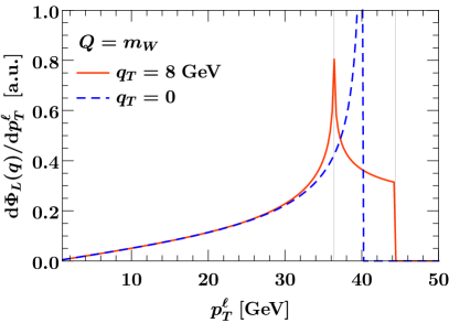
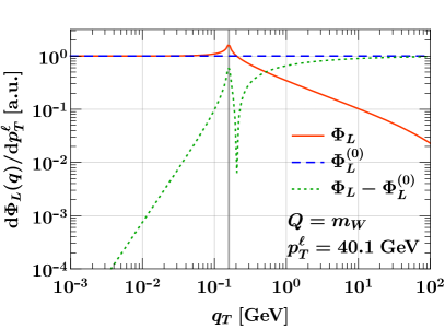
Figure -651: Leptonic phase space $\mathrm{d}\Phi_{L}(q)/\mathrm{d}p_{T}^{\ell}$, as a function of $p_{T}^{\ell}$ for fixed $q_{T}$ (left) and as a function of $q_{T}$ for fixed $p_{T}^{\ell}=40.1\,\mathrm{GeV}$ (right). In both cases we fix $Q=m_{W}=80.358\,\mathrm{GeV}$. Left: The red solid curve shows the exact result for $q_{T}=8\,\mathrm{GeV}$, and the blue dashed curve shows the $q_{T}=0$ Born limit. Right: The red solid curve shows the exact phase space, the blue dashed line the LP limit, and the green dotted curve their difference.

Clearly, expanding in $\epsilon\sim\lambda$ is only well-defined if $\kappa\ll 1$, i.e., away from the Jacobian peak $p_{T}^{\ell}\ll Q/2$. This is already evident from the divergence of eq. (4.3.1) as $\kappa\to 1$. As long as $\kappa\ll 1$, $\epsilon$ is the only small scale in the problem, which justifies expanding in $\epsilon$ and leads to at most linear fiducial power corrections. On the other hand, close to the Jacobian peak, the distance $p_{L}=Q-2p_{T}^{\ell}$ emerges as an additional small scale, and the naive expansion in $q_{T}$ is actually an expansion in $q_{T}/p_{L}$, which is only allowed for $q_{T}\ll p_{L}$ but breaks down for $p_{L}\sim q_{T}$. To illustrate this explicitly, we can expand in the regime $p_{L}\sim q_{T}$ by simultaneously counting both scales as small. To do so, we take

$$p_{L}=Q-2p_{T}^{\ell}\sim\lambda Q\,,\qquad 1-\kappa=\frac{p_{L}}{Q}\sim\lambda\,,$$ (4.22)

where as before $\epsilon=q_{T}/Q\sim\lambda$, such that formally $q_{T}/(Q-2p_{T}^{\ell})\sim 1$. With this replacement, we can expand eq. (4.19) in $\lambda$,

$$\frac{L_{i}(q,p_{T}^{\ell})}{L_{\pm(i)}(q^{2})} =\frac{3}{4\pi}\frac{1}{\sqrt{2Q}}\int_{0}^{2\pi}\!\mathrm{d}\varphi\,\frac{\theta(q_{T}\,c_{\varphi}+p_{L})}{\sqrt{q_{T}\,c_{\varphi}+p_{L}}}\,g_{i}\bigl{(}\pi/2,\varphi\bigr{)}\times\bigl{[}1+\mathcal{O}(\lambda)\bigr{]}\,.$$ (4.23)

This vanishes for all $g_{i}$ odd in $\varphi$, which only leaves $i=-1,0,2,3$. This should be contrasted with the naive LP result in eq. (4.3.1), which only receives contributions from $i=-1,0$. The $i=2$ contribution is proportional to the double-Boer-Mulders effect, which we can neglect, see the discussion below eq. (2.103). For $i=3$ we have $W_{3}\sim\mathcal{O}(\lambda)$, see table 1, which thus yields a linear power correction. Hence, we find the interesting effect that the proximity to the Jacobian peak induces sensitivity to new hadronic structure functions at $\mathcal{O}(\lambda)$, which do not contribute at $\mathcal{O}(\lambda)$ away from the peak region.

From eq. (4.23) it is evident that naively expanding in $q_{T}$ near the Jacobian peak would amount to expanding in $q_{T}/p_{L}$, which is not allowed. However, eq. (4.23) is only valid near the peak, because by counting $p_{L}/Q\sim\lambda$ we have expanded away the dependence on $\kappa=1+\mathcal{O}(\lambda)$, which is not allowed away from the peak. Hence, to cover the full range of $p_{T}^{\ell}$, we must not expand in $p_{L}$, while near the peak we must count $q_{T}\sim p_{L}$ to avoid inducing uncontrolled leptonic power corrections in $q_{T}/p_{L}$. Clearly, the simplest way to satisfy both requirements is to not expand at all and keep the exact result corresponding to eq. (4.19).

Finally, note that the breakdown of the naive power expansion around $p_{T}^{\ell}=Q/2$ does not immediately affect the leptonic tensor if we only consider a fiducial cut $p_{T}^{\ell}\geq p_{T}^{\mathrm{min}}$, since we can evaluate it as

$$\Phi_{L}(q,p_{T}^{\mathrm{min}}) =\int_{p_{T}^{\mathrm{min}}}\mathrm{d}p_{T}^{\ell}\frac{\mathrm{d}\Phi_{L}(q)}{\mathrm{d}p_{T}^{\ell}}=\frac{1}{8\pi}-\int_{0}^{p_{T}^{\mathrm{min}}}\mathrm{d}p_{T}^{\ell}\frac{\mathrm{d}\Phi_{L}(q)}{\mathrm{d}p_{T}^{\ell}}\,.$$ (4.24)

Thus, the leptonic power corrections in this case scale as $q_{T}/(Q-2p_{T}^{\mathrm{min}})$, and so as long as $p_{T}^{\mathrm{min}}\ll Q/2$, the effect of $p_{T}^{\mathrm{min}}$ can be treated as a linear fiducial power correction as discussed for the $q_{T}$ spectrum with fiducial cuts in section 4.2.

4.3.2 Numerical results

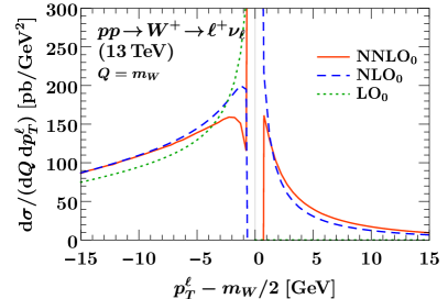
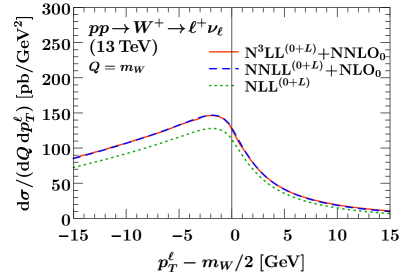
Figure -650: Lepton transverse momentum spectrum for on-resonance $W^{+}$ production at the LHC at fixed order (left) and including the resummation of fiducial power corrections to N³LL (right). The horizontal axes shows the distance to the Jacobian peak at $p_{T}^{\ell}=m_{W}/2$.

There are two key insights from our analysis of the differential $p_{T}^{\ell}$ phase space. First, the $p_{T}^{\ell}$ spectrum near the Jacobian peak is directly sensitive to the small transverse momentum $q_{T}$ of the decaying vector boson. This causes fixed-order predictions to become unreliable in this region, which is a well-known effect. Second, the strict $q_{T}\to 0$ limit by itself cannot describe the $p_{T}^{\ell}$ spectrum in this region, which means the strict LP $q_{T}$ resummation is also insufficient. Both problems are cured simultaneously by combining the exact leptonic tensor, which encodes the exact decay kinematics and automatically retains all leptonic power corrections, with the $q_{T}$-resummed hadronic tensor, thus allowing us to obtain physical predictions around the Jacobian peak.

We illustrate this in figure -650 for the $p_{T}^{\ell}$ spectrum in $W^{+}\to\ell^{+}\nu_{\ell}$ decays, where we show the spectrum both at fixed order (left) and after resummation including fiducial power corrections (right). In both panels, the horizontal axis shows the distance of $p_{T}^{\ell}$ to the Jacobian peak at $p_{T}^{\ell}=m_{W}/2$, and to avoid smearing out the peak we consider the spectrum at a fixed point $Q=m_{W}$. The fixed-order spectrum (left) is shown at LO₀ (green dotted), NLO₀ (blue dashed), and NNLO₀ (red solid). The LO₀ result corresponds to Born kinematics and clearly shows the kinematic edge at $p_{T}^{\ell}=Q/2$. Starting at NLO₀, the $W$ boson can have nonvanishing $q_{T}$, which opens up the phase space beyond the edge. However, in the vicinity of the edge, the fixed-order predictions become unstable due to the sensitivity to small $q_{T}$, which is clearly visible by the diverging NLO₀ and NNLO₀ curves, and in particular by the sign change between NLO₀ and NNLO₀ at $p_{T}^{\ell}\approx Q/2$.

In the right panel in figure -650, we show the resummed $p_{T}^{\ell}$ spectrum at NLL^(0+L) (green dotted), NNLL^(0+L)+NLO₀ (blue dashed), and N³LL^(0+L)+NNLO₀ (red solid). The resummation including leptonic power corrections cures the unphysical behaviour of the fixed-order results, yielding a well-behaved spectrum in the full $p_{T}^{\ell}$ range, with a resummed Sudakov shoulder at $p_{T}^{\ell}\approx m_{W}/2$. Note that the cross section beyond the edge is already populated at NLL^(0+L) without any fixed-order matching. We stress that without including the exact leptonic tensor, the resummation would only affect the region $p_{T}^{\ell}<m_{W}/2$, and not cure the peak region. In fact, the results with strict LP resummation would look very similar to the pure fixed-order results, with the N³LL⁽⁰⁾+NNLO₀ essentially indistinguishable from the pure NNLO₀ result.

This is the first time that resummed N³LL results for the $p_{T}^{\ell}$ spectrum are presented, and we observe extremely good perturbative convergence, with the results at NNLL^(0+L)+NLO₀ and N³LL^(0+L)+NNLO₀ falling on top of each other. We leave a more detailed phenomenological analysis of the $p_{T}^{\ell}$ spectrum to future work.

4.4 $\phi^{*}$ spectrum

The $\phi^{*}$ observable was first proposed in ref. [204], extending earlier work on the $a_{T}$ observable [205, 206]. Both observables are sensitive to small $q_{T}$, but promise better experimental resolution than $q_{T}$ itself due to being based on angular measurements, which are less susceptible to the momentum resolution of the individual lepton momenta than $q_{T}$ itself.

The factorization and resummation for $a_{T}$ was first studied in ref. [207] at NLL, and extended to both $a_{T}$ and $\phi^{*}$ at NNLL$+$NLO in refs. [208, 209, 70], and also in refs. [210] including a study of nonperturbative contributions, and also more recently at N³LL$+$NNLO in refs. [81, 83]. None of these calculations incorporate the finite recoil of the dilepton system in the calculation of the $\phi^{*}$ observable, i.e. the employed definition of $\phi^{*}$ is only an approximation of the actually measured observable, as discussed below. The resummation with the exact definition of $\phi^{*}$ was considered in refs. [73, 84] at NNLL$+$NNLO and NNLL$+$NLO via parton-level MC integration of the leptonic final state.

Ref. [204] defines the two closely related observables $\phi^{*}_{\mathrm{CS}}$ and $\phi^{*}_{\eta}$. We only consider the latter, as it is more commonly used in experiments. It is defined as

$$\phi^{*}\equiv\phi^{*}_{\eta}=\tan(\phi_{\mathrm{acop}}/2)\,\sin\theta_{\eta}^{*}\,,$$ (4.25)

where the acoplanarity angle is $\phi_{\mathrm{acop}}=\pi-\Delta\varphi$, with $\Delta\varphi$ being the azimuthal opening angle between the leptons in the lab frame, and

$$\cos\theta_{\eta}^{*}=\tanh\frac{\eta_{1}-\eta_{2}}{2}\,,$$ (4.26)

where $\eta_{1,2}$ are the two lepton rapidities.

4.4.1 Origin of power corrections

Using the parametrization of the lepton momenta in the Collins-Soper frame as given in eq. (2.55), eq. (4.25) can be written as

$$(\phi^{*})^{2} =\frac{8\kappa(\epsilon\sin\varphi\sin\theta)^{2}}{(\kappa-\epsilon^{2}+\alpha^{2})^{2}(\kappa+\epsilon^{2}-\alpha^{2}+2)}\,,$$

$$\kappa^{2} =(\epsilon^{2}-\alpha^{2})^{2}+4\epsilon^{2}\sin^{2}\theta\sin^{2}\varphi\,,\qquad\alpha^{2}=\bigl{(}1+\epsilon^{2}\cos^{2}\varphi\bigr{)}\sin^{2}\theta\,.$$ (4.27)

Note that $\phi^{*}$ is boost invariant and thus independent of $Y$, and can depend on $q_{T}$ only through the dimensionless ratio $\epsilon=q_{T}/Q$. From eq. (4.4.1), one easily finds the special values

$$\phi^{*}|_{\theta=\pi/2}=\epsilon\lvert\sin\varphi\rvert\,,\qquad\lim_{\theta\to 0,\pi}\phi^{*}=\infty\,.$$ (4.28)

The singularity arises from the case where both momenta are parallel to each other in the transverse plane, such that $\phi_{\rm acop}=\pi$ and eq. (4.25) becomes ill-defined. Numerically, we have also tested that $\phi^{*}$ monotonically decreases with $|\!\sin\theta|$, such that $\phi^{*}$ can be uniquely inverted on the intervals $\theta\in[0,\pi/2]$ and $\theta\in[\pi/2,\pi]$, with the two solutions trivially related by $\theta_{1}=\pi-\theta_{2}$.

Expanding eq. (4.4.1) in $\epsilon\ll 1$, one obtains the commonly employed approximation

$$\phi^{*\,(0)}=\epsilon\,\lvert\sin\varphi\rvert\,.$$ (4.29)

The monotonicity of $\phi^{*}$ with $\lvert\sin\theta\rvert$ implies that this is a lower bound to $\phi^{*}$, but from eq. (4.28) it follows that this bound is only saturated for $\theta=\pi/2$. It is thus natural to ask whether there is a better approximation of $\phi^{*}$. From eq. (4.4.1), it is easy to see that $\phi^{*}$ only vanishes if either $\epsilon=0$ or $\sin\varphi=0$. Expanding eq. (4.4.1) in these limits, we find

$$(\phi^{*})^{2} =\frac{\epsilon^{2}\sin^{2}\varphi}{1+\epsilon^{2}(1-\sin^{-2}\theta)}+\mathcal{O}(\sin^{4}\varphi)$$

$$=\epsilon^{2}\sin^{2}\varphi\bigl{[}1+\epsilon^{2}\cot^{2}\theta+\,\mathcal{O}(\epsilon^{4})\bigr{]}\,.$$ (4.30)

Note that the expansion in small $\epsilon$ in the second line can be recovered by reexpanding the small-$\sin\varphi$ limit, because in eq. (4.4.1) each term in $\epsilon$ either multiplies $\sin\varphi$ or is enhanced relative to $\epsilon\sin\varphi$. The first line in eq. (4.4.1) is ill-defined for $\lvert\tan\theta\rvert<\epsilon$ already at the leading $\mathcal{O}(\sin^{2}\varphi)$, while this singularity only appears at the second order in $\epsilon$. Eq. (4.4.1) suggests that the fundamentally small quantity to be power counted is $\epsilon\lvert\sin\varphi\rvert$, not $\epsilon$ itself. In particular, any given value in $\phi^{*}$ can in principle receive contributions from arbitrarily large $\epsilon$.

In figure -649, we compare the exact result for $\phi^{*}$ (red solid) to its leading expansions in small $\sin\varphi$ (blue dashed) and small $\epsilon$ (green dotted). We fix $\varphi=\pi/8$ and show results for $\epsilon=0.25$ (left panel) and $\epsilon=0.5$ (right panel). The gray vertical line shows the breakdown of the small-$\sin\varphi$ approximation at $\cos\theta=(1+\epsilon^{2})^{-1/2}$. Since $\phi^{*}$ is fairly insensitive to $\cos\theta$ in a rather large range of $\cos\theta$, the small-$\epsilon$ expansion is a fairly good approximation in that region. However, it quickly deteriorates for moderate to large $\cos\theta$. In contrast, the small-$\sin\varphi$ expansions follows the exact curve remarkably well, almost up to the point where it becomes ill-defined. At large $\cos\theta$, both approximations break down, as $\phi^{*}$ is driven by the small-$\theta$ behavior $\phi^{*}\sim 1/\theta^{2}$.

We find that the region $\lvert\tan\theta\rvert<\epsilon$ cannot be described by the expansion in small-$\sin\varphi$, which breaks down, or by the expansion small-$\epsilon$, which assigns an artificially small value $\phi^{*(0)}$ in this region. However, this does not invalidate the LP description of $\phi^{*}$, as this region of phase space is suppressed as $\mathcal{O}(\epsilon^{2})$,

$$\int\mathrm{d}\Phi_{L}(q)\,\theta(\lvert\tan\theta\rvert<\epsilon)=\frac{1}{8\pi}\bigl{(}1-\sqrt{1-\epsilon^{2}}\bigr{)}=\frac{\epsilon^{2}}{16\pi}+\mathcal{O}(\epsilon^{4})\,.$$ (4.31)

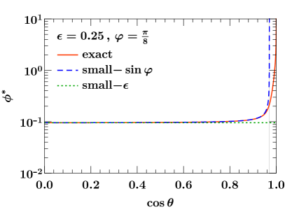
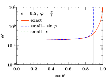
Figure -649: Comparison of the different expansions of $\phi^{*}$, as given in eq. (4.4.1), as function of $\cos\theta$ for two different choices of $\epsilon$ and $\varphi$. The vertical gray line indicates the breakdown of the expansion in small $\sin\varphi$.

Another important property of $\phi^{*}$ is that it is not azimuthally symmetric at LP due to its explicit dependence on $\varphi$. To identify which $W_{i}$ contribute to $\phi^{*}$ at LP, we evaluate eq. (2.60) with the approximate observable in eq. (4.29), which yields

$$\frac{\mathrm{d}\sigma}{\mathrm{d}Q^{2}\mathrm{d}Y\mathrm{d}\!\cos\theta\,\mathrm{d}\phi^{*{(0)}}} =\frac{3Q}{16\pi E_{\mathrm{cm}}^{2}}\sum_{i=-1,0,2,4}L_{\pm(i)}(Q^{2})\,g_{i}(\theta,0)$$

$$\quad\times\int_{0}^{\infty}\mathrm{d}b_{T}\,K_{i}(b_{T}Q\phi^{*{(0)}})\tilde{W}_{i}(Q^{2},Y,b_{T})\,.$$ (4.32)

Here, the $\tilde{W}_{i}$ are the hadronic structure functions in Fourier space. In eq. (4.4.1), we have already carried out the integral over $\varphi$, which gives rise to kernels $K_{i}$, while we are still differential in $\cos\theta$. One can easily incorporate any LP fiducial cuts that depend on $\theta$, but are independent of $\varphi$ into eq. (4.4.1), which holds for most common cuts such as eq. (4.5).

The nonvanishing kernels entering eq. (4.4.1) are given by

$$K_{-1,0,4}(\beta) =\cos(\beta)\,,\qquad K_{2}(\beta)=\cos(\beta)+2\beta\operatorname{si}(\beta)\,,$$ (4.33)

where $\operatorname{si}(\beta)=-\int_{\beta}^{\infty}\!\mathrm{d}t\,\sin t/t$ is the sine integral. The kernels for $i=1,3,5,6,7$ vanish because the corresponding $g_{i}(\theta,\varphi)$ are odd in $\varphi$ or under $\varphi\to\varphi+\pi$. Since $g_{-1,0,4}(\theta,\varphi)$ are independent of $\varphi$, they give rise to the same kernel $K_{-1,0,4}$. In contrast, $W_{2}$ is dressed with a different kernel $K_{2}$ due to the nontrivial $\varphi$ dependence of $g_{2}(\theta,\varphi)\propto\cos(2\varphi)$. In particular, for $\beta\to\infty$ one has $K_{2}(\beta)\approx-\cos\beta=K_{-1,0,4}(\beta)$, and thus there is a relative phase shift of $\pi$.

Eq. (4.4.1) is convenient, as it effectively only reweights the (resummed) hadronic tensor in Fourier space with $K_{i}(b_{T}Q\phi^{*})$, compared to $J_{0}(b_{T}q_{T})$ appearing in $q_{T}$ resummation. In momentum space, this is equivalent to the fact that the spectrum for the LP $\phi^{*{(0)}}$ in eq. (4.29) can be obtained by reweighting the (resummed) $q_{T}$ distribution with the angle to the dilepton system. The convenient form of eq. (4.4.1) was first noticed in refs. [207, 208], where it was also noted that the $\cos(b_{T}Q\phi^{*})$ gives rise to a plateau in the resummed $\phi^{*}$ spectrum, in contrast to the Sudakov peak encountered in $q_{T}$ resummation. However, the form in eq. (4.4.1) has the distinct disadvantage that it does not allow one any longer to include fiducial power corrections due to additional fiducial cuts beyond the strict LP.

The above previous works did not consider the contribution from $W_{2}^{(0)}$, which involves the double-Boer-Mulders contribution, see eq. (2.103). Comparing to table 1, $W_{2}$ does not contribute to azimuthally symmetric observables at LP, and thus is not encountered in the LP ${\vec{q}}_{T}$ resummation. In practice, we expect this contribution to be rather small, as $h_{1}^{\perp}$ only matches onto subleading twist-3 collinear PDFs, and thus we will not consider it in our numerical study. Nevertheless, it is interesting to note that the $\phi^{*}$ spectrum may give direct access to the double Boer-Mulders effect, and we leave a more detailed study of this for future work. At leading twist-2, $W_{2}$ is suppressed as $\mathcal{O}(\lambda^{2})$, such that our resummed spectrum $\sigma^{(0+L)}$ still fully captures all linear power corrections arising from small $q_{T}$ with leading-twist collinear PDFs, and this also holds when including additional fiducial cuts.

4.4.2 Numerical results

We now turn to the numerical study of power corrections to $\phi^{*}$ at one loop. For simplicity, we work at fixed $Q=m_{Z}$, and normalize all results to the tree-level cross section. The results for inclusive and fiducial Drell-Yan are shown in the left and right panel of figure -648, respectively. In both plots, the exact results $\sigma$ are shown by the red points, the factorized prediction including fiducial power corrections $\sigma^{(0+L)}$ by the blue line, and their difference by the green dot-dashed curve. This is contrasted by the gray-dashed curve which shows the difference $\sigma-\sigma^{(0)}$ between the exact and strict LP (i.e. employing $\phi^{*(0)}$) result. The orange, dot-dashed curve shows the difference $\sigma^{(0+L)}_{\rm GJ}-\sigma^{(0+L)}$ between our default CS tensor decomposition, and an alternative choice corresponding to the GJ frame.

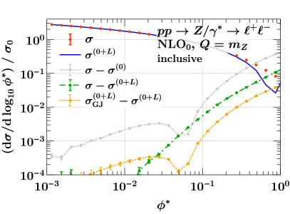
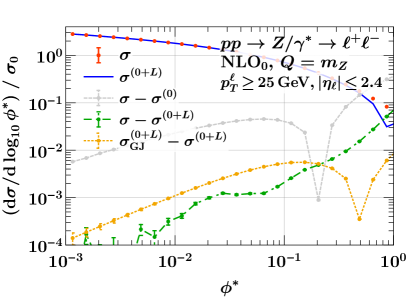
Figure -648: Power corrections for $\phi^{*}$ for inclusive (left) and fiducial (right) Drell-Yan production.

In the inclusive case (left panel), $\sigma^{(0+L)}$ and $\sigma^{(0)}$ only differ by whether $\phi^{*}$ is implemented exactly or using $\phi^{*(0)}$. In this case, we observe large linear corrections to $\sigma^{(0)}$, whereas corrections to $\sigma^{(0+L)}$ appear to be quadratically suppressed. Interestingly, the $\sigma^{(0+L)}_{\rm GJ}$ seems to have linear corrections as can be seen from the linear scaling of the difference $\sigma^{(0+L)}_{\rm GJ}-\sigma^{(0+L)}$. Hence, $\sigma^{(0+L)}$ for a generic frame receives linear corrections, although they are roughly an order of magnitude suppressed compared to $\sigma^{(0)}$.

For fiducial Drell-Yan production (right panel), we observe linear power corrections for both $\sigma^{(0)}$ and $\sigma^{(0+L)}$, which are larger than the power corrections in the inclusive case, especially for $\sigma^{(0)}$. Nevertheless, we again see see that $\sigma^{(0+L)}$ has significantly smaller corrections than $\sigma^{(0)}$, despite having the same linear scaling in $\phi^{*}$. The ambiguity between the two choices of tensor decomposition is again a linear effect, but again at much smaller overall magnitude than the corrections beyond $\sigma^{(0)}$.

Overall, we find that $\phi^{*}$ generically receives linear power corrections. In addition to the common fiducial corrections, $\phi^{*}$ is affected by corrections from expanding the observable itself, and by the fact that even very small $\phi^{*}$ receives contributions from large $q_{T}$, as is apparent from eq. (4.29). Hence, a priori there is no reason to expect that corrections to $\phi^{*}$ are quadratically suppressed. Nevertheless, $\sigma^{(0+L)}$ includes all linear power corrections from small-$q_{T}$, which is reflected by the corrections to $\sigma^{(0+L)}$ being significantly reduced compared to $\sigma^{(0)}$. We also note that the choice of tensor decomposition strongly affects how well contributions from large $q_{T}$ are captured. Empirically, we find that our default choice corresponding to the CS frame minimizes the size of power corrections, but we have not been able to identify an underlying reason for this observation.

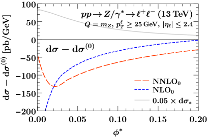
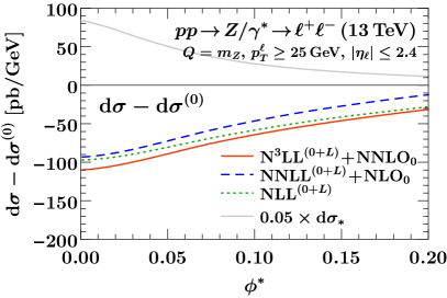
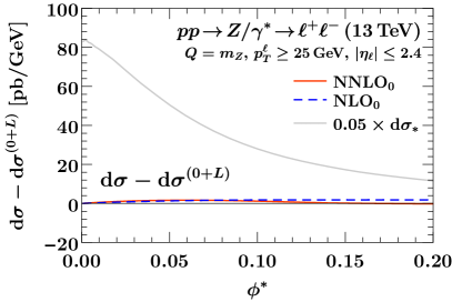
Figure -647: Subleading-power contributions to the fiducial $\phi^{*}$ spectrum for Drell-Yan on the resonance, $Q=m_{Z}$. We compare the sum of all subleading power contributions, treating the linear fiducial power corrections at fixed order (top left) or resumming them to all orders (top right). Our best prediction $\mathrm{d}\sigma_{*}$ for the total spectrum at N³LL${}^{(0+L)}+$NNLO₀ is indicated as a light gray line for reference, scaled down to $5\%$ of its original size. The bottom panel shows the remaining fixed-order power corrections, which are finite for $\phi^{*}\to 0$ (note the difference in vertical scale).

We conclude this section by studying the impact of the fiducial power corrections on the resummed $\phi^{*}$ spectrum with fiducial cuts. In the top-left panel of figure -647, we show the difference between the strict LP and the exact $\phi^{*}$ spectrum at NLO₀ (blue, short-dashed) and NNLO₀ (red, long-dashed). For reference, the gray line shows our best prediction $\sigma_{*}$ at N³LL${}^{(L)}+$NNLO₀, scaled down to 5$\%$ of its original size. We note a large discrepancy between NLO₀ and NNLO₀ as $\phi^{*}\to 0$, indicating large, unresummed logarithms in the power corrections and consequently poor perturbative convergence in this regime.

In the top-right panel of figure -647, we show the difference between the LP $\phi^{*}$ spectrum and the resummed and matched $\phi^{*}$ spectrum, at NLL^(0+L) (green, dotted), NNLL${}^{(0+L)}+$NLO₀ (blue, dashed) and N³LL${}^{(0+L)}+$NNLO₀ (red, solid), which corresponds to the left panel but with the linear power corrections resummed. As a result, the divergence as $\phi^{*}\to 0$ is cured, and we observe very good perturbative convergence between the different resummed predictions. Note that in contrast to $q_{T}$, see figure -652, the resummed power corrections do not vanish as $\phi^{*}\to 0$, due to the different weighting of the Sudakov factor with $\cos(b_{T}Q\phi^{*})$ rather than $J_{0}(b_{T}q_{T})$, cf. eq. (4.4.1).

Finally, in the bottom panel of figure -647 we show the remaining fixed-order power corrections after including the fiducial power corrections in the resummation at NLO₀ (blue, short-dashed) and NNLO₀ (red solid), again including our best prediction $\sigma_{*}$ for reference. Since all terms diverging as $\phi^{*}\to 0$ are included in $\sigma^{(0+L)}$, the remaining power corrections are well-behaved as $\phi^{*}\to 0$, which makes their overall size almost negligible.

5 Applications in fixed-order subtractions

The inclusion of fiducial power corrections in the $q_{T}$ factorization theorem by treating the leptonic tensor exactly can be immediately applied to improve the $q_{T}$ subtraction method. In fact, we have employed this in section 4.3 to obtain NNLO predictions for the $p_{T}^{\ell}$ spectrum. Here, we elaborate in more detail on this, illustrating that this approach can significantly and systematically improve the $q_{T}$ subtraction. In particular, it becomes crucial in regions of phase space sensitive to leptonic power corrections, such as $p_{T}^{\ell}$ close to the Jacobian peak, where the strict LP expansion breaks down, and thereby also the subtractions based on the strict LP limit.

5.1 $q_{T}$ subtraction with fiducial power corrections

The $q_{T}$ subtraction method has been originally proposed in ref. [115] for the calculation of color-singlet processes at NNLO, and its application at N³LO was discussed in refs. [211, 178]. Here, we briefly review this method, and discuss how to extend it to include fiducial power corrections. Here, we only discuss the simplest implementation of $q_{T}$ subtractions as a phase-space slicing. As discussed in ref. [104], fiducial cuts can also be explicitly accounted for in a differential implementation of $q_{T}$ subtractions, which can also be further improved with the methods we discuss here, which we leave for future work.

We denote the cross section to be calculated as $\sigma(X)$, where $X$ summarizes all observables to be differential in, such as $Q$, $Y$, and $p_{T}^{\ell}$, as well as possible fiducial cuts. The cross section can be written as

$$\sigma(X) =\int_{0}^{\infty}\mathrm{d}q_{T}\,\frac{\mathrm{d}\sigma(X)}{\mathrm{d}q_{T}}=\sigma(X,q_{T}^{\mathrm{cut}})+\int_{q_{T}^{\mathrm{cut}}}^{\infty}\mathrm{d}q_{T}\,\frac{\mathrm{d}\sigma(X)}{\mathrm{d}q_{T}}\,,$$ (5.1)

where the cumulative cross section as a function of $q_{T}^{\mathrm{cut}}$ is defined as

$$\sigma(X,q_{T}^{\mathrm{cut}})=\int_{0}^{q_{T}^{\mathrm{cut}}}\mathrm{d}q_{T}\,\frac{\mathrm{d}\sigma(X)}{\mathrm{d}q_{T}}\,.$$ (5.2)

The $q_{T}$ subtraction is typically implemented as a slicing method by adding and subtracting a suitable subtraction term,

$$\sigma(X) =\sigma^{\mathrm{sub}}(X,q_{T}^{\mathrm{cut}})+\int_{q_{T}^{\mathrm{cut}}}^{\infty}\mathrm{d}q_{T}\,\frac{\mathrm{d}\sigma(X)}{\mathrm{d}q_{T}}+\Delta\sigma(X,q_{T}^{\mathrm{cut}})\,,$$

$$\Delta\sigma(X,q_{T}^{\mathrm{cut}}) =\sigma(X,q_{T}^{\mathrm{cut}})-\sigma^{\mathrm{sub}}(X,q_{T}^{\mathrm{cut}})\,.$$ (5.3)

For color-singlet processes, $q_{T}$ vanishes by construction in the Born limit. Hence, the integral in eq. (5.1) necessarily involves at least one resolved real emission, and can thus be calculated from the corresponding Born$+1$-parton process at one order lower than $\sigma(X)$ itself. The cancellation of virtual and real divergences occurs only in the limit $q_{T}\to 0$. By constructing $\sigma^{\mathrm{sub}}$ such that it fully describes this limit, the cancellation of IR divergences only occurs within $\sigma^{\mathrm{sub}}$, and $\Delta\sigma$ is a power correction that vanishes as $q_{T}^{\mathrm{cut}}\to 0$, and thus can be neglected for sufficiently small values of $q_{T}^{\mathrm{cut}}$.

To construct $\sigma^{\mathrm{sub}}$ and study the size of $\Delta\sigma$, it is useful to expand the differential cross section and its cumulant for $q_{T}\ll Q$ and $q_{T}^{\mathrm{cut}}\ll Q$, respectively,

$$\frac{\mathrm{d}\sigma(X)}{\mathrm{d}q_{T}} =\frac{\mathrm{d}\sigma^{(0)}(X)}{\mathrm{d}q_{T}} +\sum_{m>0}\frac{\mathrm{d}\sigma^{(m)}(X)}{\mathrm{d}q_{T}}\,,$$ (5.4)

$$\sigma(X,q_{T}^{\mathrm{cut}}) =\sigma^{(0)}(X,q_{T}^{\mathrm{cut}}) +\sum_{m>0}\sigma^{(m)}(X,q_{T}^{\mathrm{cut}})\,,$$

where the different contributions scale as

$$\frac{\mathrm{d}\sigma^{(0)}(X)}{\mathrm{d}q_{T}} \sim\delta(q_{T})+\sum_{j\geq 0}\biggl{[}\frac{\ln^{j}(q_{T}/Q)}{q_{T}}\biggr{]}_{+}\,,\quad \sigma^{(0)}(X,q_{T}^{\mathrm{cut}}) \sim\sum_{j\geq 0}\ln^{j}\frac{q_{T}^{\mathrm{cut}}}{Q}\,,$$

$$q_{T}\frac{\mathrm{d}\sigma^{(m)}(X)}{\mathrm{d}q_{T}} \sim\Bigr{(}\frac{q_{T}}{Q}\Bigl{)}^{m}\,\sum_{j\geq 0}\ln^{j}\frac{q_{T}}{Q}\,, \sigma^{(m)}(X,q_{T}^{\mathrm{cut}}) \sim\Bigl{(}\frac{q_{T}^{\mathrm{cut}}}{Q}\Bigr{)}^{m}\,\sum_{j\geq 0}\ln^{j}\frac{q_{T}^{\mathrm{cut}}}{Q}\,.$$ (5.5)

The $\mathrm{d}\sigma^{(0)}/\mathrm{d}q_{T}$ diverges as $1/q_{T}$ for $q_{T}\to 0$, and is in fact precisely given by the factorization theorem in eq. (2.103). Note that it contains $\delta$ and plus distributions to regulate this divergence, which precisely encodes the cancellation of virtual and real IR divergences. The $\mathrm{d}\sigma^{(m)}/\mathrm{d}q_{T}$ with $m>0$ are integrable as $q_{T}\to 0$, and consequently $\sigma^{(m)}(q_{T}^{\mathrm{cut}}\to 0)\to 0$.

The subtraction term $\sigma^{\mathrm{sub}}(X,q_{T}^{\mathrm{cut}})$ must contain all singular terms, and has the form

$$\sigma^{\mathrm{sub}}(X,q_{T}^{\mathrm{cut}}) =\sigma^{(0)}(X,q_{T}^{\mathrm{cut}})\times\bigl{[}1+\mathcal{O}(q_{T}^{\mathrm{cut}}/Q)\bigr{]}\,.$$ (5.6)

It follows that the correction term in eq. (5.1) scales as

$$\Delta\sigma(X,q_{T}^{\mathrm{cut}}) =\sigma(q_{T}^{\mathrm{cut}})-\sigma^{\mathrm{sub}}(X,q_{T}^{\mathrm{cut}})=\mathcal{O}\bigl{[}(q_{T}^{\mathrm{cut}}/Q)^{m}\bigr{]}\,,$$ (5.7)

where $m$ corresponds to the first term in the sum in eq. (5.4) that is not contained in $\sigma^{\mathrm{sub}}$. So far, $q_{T}$ subtractions have always been implemented in this fashion by choosing $\sigma^{\mathrm{sub}}=\sigma^{(0)}$.

As discussed in section 2, for inclusive processes the sum in eq. (5.4) starts with $m=2$, i.e. $\Delta\sigma$ is suppressed as $\mathcal{O}(q_{T}^{2}/Q^{2}$). These terms were explicitly calculated in ref. [160] for Higgs and Drell-Yan production differential in $Q$ and $Y$, but inclusive in their decay. The corresponding results for inclusive Higgs and Drell-Yan production, i.e. integrated over $Y$, were also calculated later in refs. [212, 139].

When applying fiducial cuts, one expects corrections to be only suppressed as $\mathcal{O}(q_{T}/Q)$, i.e. $m=1$, as shown in ref. [104] and discussed more generally in sections 2 and 4. In section 4, we also demonstrated that more complicated observables such as $p_{T}^{\ell}$ or $\phi^{*}$ can also have much larger corrections than expected.

In section 2, we showed that the linear power corrections in $q_{T}/Q$ are unique for any observables that are azimuthally symmetric in the $q_{T}\to 0$ limit, in which case they only arise from the leptonic tensor. Since the subtraction method is inherently tied to a calculation at leading-twist in collinear factorization, this also holds for more complicated observables such as $\phi^{*}$. This means that in many relevant cases the $\mathrm{d}\sigma^{(1)}/\mathrm{d}q_{T}$ term in eq. (5.4) can be unambiguously predicted and included in the subtraction term. Hence, instead of eq. (5.6) we use

$$\sigma^{\mathrm{sub}}(X,q_{T}^{\mathrm{cut}}) =\sigma^{(0+L)}(X,q_{T}^{\mathrm{cut}})\times\bigl{\{}1+\mathcal{O}\bigl{[}(q_{T}^{\mathrm{cut}}/Q)^{2}\bigr{]}\bigr{\}}\,.$$ (5.8)

where $\sigma^{(0+L)}$ includes all fiducial power corrections using our default CS tensor decomposition. In principle, other choices are possible as well. From our discussion of $\phi^{*}$ in section 4.4, we have some indication that the CS decomposition tends to minimize the power corrections in more complicated cases, which motivates using it as our default choice also in the subtraction context.

5.2 Application to the lepton $p_{T}$ spectrum

We illustrate the advantage of including the leptonic corrections in eq. (5.8) for the case of the $p_{T}^{\ell}$ spectrum. As discussed in section 4.3 (see e.g. figure -651), we can distinguish three regions in the spectrum according to their sensitivity to small $q_{T}$. The expected dependence on $q_{T}^{\mathrm{cut}}$ and the linear subtraction terms are as follows:

1. Sufficiently below the Jacobian peak, $p_{T}^{\ell}\lesssim(m_{W}-q_{T}^{\mathrm{cut}})/2$, only quadratic power corrections arise, and thus we expect no significant impact from including the linear terms in the subtraction.

2. Around the Jacobian peak, $|2m_{W}-p_{T}^{\ell}|\lesssim q_{T}^{\mathrm{cut}}$, the standard power counting breaks down, and one is sensitive to the singular behavior as $q_{T}\to 0$. In this region, keeping fiducial power corrections becomes strictly necessary, since the strict LP expansion breaks down due to leptonic power corrections $q_{T}/(2m_{W}-p_{T}^{\ell})$. In particular, the region $m_{W}/2<p_{T}^{\ell}<(m_{W}+q_{T}^{\mathrm{cut}})/2$ requires to take these corrections into account, as otherwise the singular prediction is limited to $p_{T}^{\ell}<m_{W}/2$, and the region beyond the peak will contain leftover singular behavior.

3. Far above the Jacobian peak, $p_{T}^{\ell}\gtrsim(m_{W}+q_{T}^{\mathrm{cut}})/2$, there are no contributions from the subtraction term, and only the above-cut integral in eq. (5.1) is relevant.

We illustrate these effects numerically at NLO. Reference results are obtained by evaluating $pp\to W^{+}\to\ell^{+}\nu_{\ell}$ at NLO using MCFM, which employs Catani-Seymour dipole subtractions [213, 214]. The corresponding results using $q_{T}$ subtraction are obtained by combining the below-cut contribution $\mathrm{d}\sigma^{\mathrm{sub}}/\mathrm{d}p_{T}^{\ell}$ obtained from SCETlib, both for $\sigma^{\mathrm{sub}}=\sigma^{(0)}$ and $\sigma^{\mathrm{sub}}=\sigma^{(0+L)}$, with the above-cut contribution obtained by evaluating $pp\to(W^{+}{\to}\ell^{+}\nu_{\ell})+1$ parton at LO₁ using MCFM. We work in the narrow-width approximation such that $Q=m_{W}$, which avoids smearing out the Jacobian peak, as is necessary to clearly see the effects described above. To keep numerical uncertainties from the Monte Carlo integration small, we bin the $p_{T}^{\ell}$ spectrum in bins of width $1~{}\,\mathrm{GeV}$, with $p_{T}^{\ell}=m_{W}/2$ being aligned with a bin boundary to cleanly separate below-peak and above-peak bins.

In figure -646, we show the relative difference for the $p_{T}^{\ell}$ spectrum obtained with $q_{T}$ subtraction to the exact NLO result, so smaller values imply that the $q_{T}$ subtractions work better with smaller missing power corrections. We show results for the two values $q_{T}^{\mathrm{cut}}=0.4~{}\,\mathrm{GeV}$ (left) and $q_{T}^{\mathrm{cut}}=1.6~{}\,\mathrm{GeV}$ (right). In the top row, we are inclusive in the lepton, while in the bottom row we apply the cuts $p_{T}^{\ell}\geq 25~{}\,\mathrm{GeV},|\eta_{\ell}|<2.4$. The blue points use the strict LP subtractions, while the red points include the fiducial power corrections in the subtraction. The error bands indicate the MC integration uncertainties. For reference, we also show the exact NLO spectrum in gray in arbitrary units.

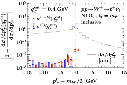
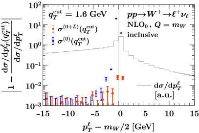
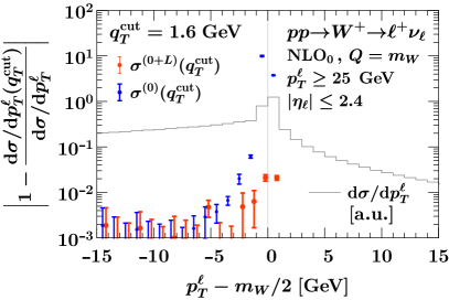
Figure -646: Relative difference of the $p_{T}^{\ell}$ spectrum obtained using $q_{T}$ subtraction to the exact NLO results, for $q_{T}^{\mathrm{cut}}=0.4~{}\,\mathrm{GeV}$ (left) and $q_{T}^{\mathrm{cut}}=1.6~{}\,\mathrm{GeV}$ (right). In the top row, we are inclusive in the lepton phase space, while in the bottom row we apply the CMS cuts $p_{T}^{\ell}\geq 25~{}\,\mathrm{GeV},|\eta_{\ell}|<2.4$. The error bands indicate uncertainties from the Monte Carlo integration. In all plots, the gray line shows the shape of the exact NLO result in arbitrary units, and the blue error bars are slightly shifted to right for better visibility only.

Due to the rather large bin size of $1\,\mathrm{GeV}$, only the two bins adjacent to the Jacobian peak at $p_{T}^{\ell}=m_{W}/2$ are significantly affected by the choice of $q_{T}^{\mathrm{cut}}$. Below the first bin left of the peak, power corrections are essentially negligible for all choices of $q_{T}^{\mathrm{cut}}$, irrespective of whether or not the fiducial power corrections are included and independent of the cuts. Beyond the first bin right to the peak, there is no contribution from the subtraction term, and the spectrum is entirely given by the above-cut contribution. However, as expected, the bins adjacent to the Jacobian peak are significantly affected by the large leptonic power corrections. At strict LP (blue points), these are of $\mathcal{O}(80\%)$ for $q_{T}^{\mathrm{cut}}=0.4~{}\,\mathrm{GeV}$, and even of $\mathcal{O}(10)$ for $q_{T}^{\mathrm{cut}}=1.6~{}\,\mathrm{GeV}$, indicating the breakdown of the subtractions. Including the fiducial power corrections (red points) automatically retains all leptonic power corrections and as a result the power corrections are of the order of a few percent, leading to stable predictions even very close to the peak. The results with and without addition fiducial cuts are very similar, as expected by the absence of linear fiducial power corrections when being inclusive in the neutrino.

Figure -645 shows the $q_{T}^{\mathrm{cut}}$ dependence of the lepton $p_{T}$ spectrum, for the bin $-1\leq p_{T}^{\ell}-\frac{m_{W}}{2}\leq-\frac{1}{2}~{}\,\mathrm{GeV}$ (left), and the bin $-\frac{1}{2}\leq p_{T}^{\ell}-\frac{m_{W}}{2}\leq 0~{}\,\mathrm{GeV}$ (right), i.e. the two bins left to the Jacobian peak. (Note the finer bin width of $0.5\,\mathrm{GeV}$, compared to $1\,\mathrm{GeV}$ above). The result for the first bin right of the peak is very similar to the right figure, while bins further away have negligible $q_{T}^{\mathrm{cut}}$ dependence that is entirely driven by MC integration uncertainties, and hence we do not explicitly show these. We also only show the inclusive case. In figure -645, we show the relative difference of the result obtained using $q_{T}$ subtractions to the MCFM result using Catani-Seymour subtractions. As before, the blue and red points correspond to implementing the $q_{T}$ subtractions without and with fiducial power corrections, and the error bars indicate MC integration uncertainties.

In the lower bin (left panel), the $q_{T}^{\mathrm{cut}}$ dependence of the $q_{T}$ subtraction including fiducial power corrections (red points) is consistent with zero within the MC uncertainties, illustrating the extremely good convergence of the subtractions. In contrast, at strict LP (blue points) there is a sizable difference to the exact result. While it is falling with $q_{T}^{\mathrm{cut}}$, one needs a very small value $q_{T}^{\mathrm{cut}}\sim 0.2-0.4\,\mathrm{GeV}$ to achieve an accuracy of $\mathcal{O}(10^{-2})$. In the bin adjacent to the peak (right figure; note the different plot range), the difference between Catani-Seymour and strict-LP $q_{T}$-subtraction results is consistently larger by a factor $\sim 10^{2}$, indicating the much stronger sensitivity to small $q_{T}\sim p_{T}^{\ell}-m_{W}/2$. As before, at strict LP (blue points) there is a strong dependence on $q_{T}^{\mathrm{cut}}$, but even at the extremely small value of $q_{T}^{\mathrm{cut}}=0.1\,\mathrm{GeV}$ the result has an $\mathcal{O}(1)$ uncertainty due to missing power corrections, showing the breakdown of the method. After including the fiducial power corrections (red points) the $q_{T}^{\mathrm{cut}}$ dependence is negligible within the MC integration uncertainties.

Note that there seems to be a systematic difference compared to the MCFM result obtained with Catani-Seymour subtractions. However, in this extreme region of phase space it is not a priori clear which of the results is more reliable and whether the reported MC uncertainties are still trustworthy. Thus, we refrain from a definite statement which subtraction method performs better in this scenario.

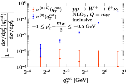
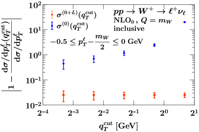
Figure -645: Relative difference of $p_{T}^{\ell}$ spectrum obtained with $q_{T}$ subtractions as a function of $q_{T}^{\mathrm{cut}}$ compared to Catani-Seymour subtractions. The two panels show two different bins in $p_{T}^{\ell}$ near the Jacobian peak, as indicated. The $q_{T}$ subtraction are implement at strict LP (blue points) and including fiducial power corrections (red points). The error bars indicate the MC integration uncertainties.

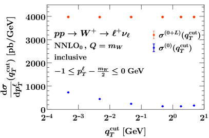
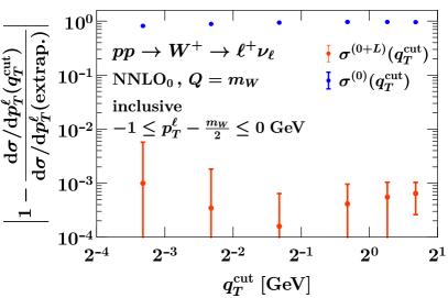
Figure -644: $q_{T}^{\mathrm{cut}}$ dependence of the $p_{T}^{\ell}$ cross section in the bin $-1\leq m_{W}/2\leq 0~{}\,\mathrm{GeV}$ with ($\sigma^{(0+L)}$, red points) and without ($\sigma^{(0)}$, blue points) fiducial power corrections included in the subtractions. In the left, we show the corresponding absolute cross sections in this bin, in the right we show their relative difference to a quadratic extrapolation of the $q_{T}^{\mathrm{cut}}$ dependence of $\sigma^{(0+L)}$.

Our numerical checks confirm the theoretical observation that close to the peak, where one is sensitive to small $q_{T}$, reliable predictions can only be obtained when taking the fiducial power corrections into account. In bins sufficiently far away from the peak, this is not as crucial, but can still significantly improve convergence of the method, i.e. it allows one to use much larger values of $q_{T}^{\mathrm{cut}}$ than the strict LP subtraction whenever linear fiducial corrections are present. This becomes particularly important at higher orders, where it becomes numerically challenging to push $q_{T}^{\mathrm{cut}}$ to such small values.

In our analysis in section 4.3, we require the $p_{T}^{\ell}$ spectrum at NNLO₀, which we obtain by combining the NLO₁ calculation of $pp\to W^{+}+1$ parton from MCFM with a $q_{T}$ subtraction including fiducial power corrections supplied by SCETlib, choosing $q_{T}^{\mathrm{cut}}=0.8\,\mathrm{GeV}$. We verify that this yields a sufficiently precise result in the first bin left of the Jacobian edge, $-1\leq m_{W}/2\leq 0~{}\,\mathrm{GeV}$. Compared to above we have increased the bin width from $0.5\,\mathrm{GeV}$ to $1\,\mathrm{GeV}$ to reduce numerical uncertainties. In the left panel in figure -644, we show the absolute cross section in this bin as a function of $q_{T}^{\mathrm{cut}}$ for $\sigma^{(0+L)}$ (red points) and $\sigma^{(0)}$ (blue points). Clearly, only the result using $\sigma^{(0+L)}$ shows a stable convergent behavior by giving a result insensitive to $q_{T}^{\mathrm{cut}}$, whereas the result for $\sigma^{(0)}$ does not converge and is quite far from the true result. We then use a simple quadratic extrapolation of $\sigma^{(0+L)}(q_{T}^{\mathrm{cut}})$ to $q_{T}^{\mathrm{cut}}\to 0$ as a proxy for the exact result in this bin. In the right figure, we show the relative difference of $\sigma^{(0+L)}$ (red points) and $\sigma^{(0)}$ (blue points) to this extrapolation. As expected, $\sigma^{(0)}$ shows $\mathcal{O}(1)$ deviations due to the clear lack of convergence towards small $q_{T}^{\mathrm{cut}}$ due to uncontrolled leptonic power corrections. In contrast, $\sigma^{(0+L)}$ is in good agreement with the extrapolation, with deviations of $\mathcal{O}(10^{-3})$ that are largely driven by numerical uncertainties. This justifies our choice of $q_{T}^{\mathrm{cut}}=0.8\,\mathrm{GeV}$ for the results presented in section 4.3. It also confirms the expectation that the systematic pattern of improvement from including fiducial power corrections in the subtractions observed at NLO₀ will carry over to NNLO₀. We leave a more detailed investigation at NNLO₀ to future work.

5.3 Application to Drell-Yan with symmetric cuts

As a second application to illustrate the $q_{T}$ subtraction including fiducial power corrections, we consider Drell-Yan $pp\to Z/\gamma^{*}\to\ell^{+}\ell^{-}$ with fiducial cuts on the final-state leptons. In particular, we focus on enhanced power corrections that arise when one applies symmetric cuts, where both leptons are required to have $p_{T}^{\ell}\geq p_{T}^{\mathrm{min}}$. For this case, it was already remarked in ref. [117] that the $q_{T}$ subtractions become very sensitive to $q_{T}^{\mathrm{cut}}$ leading to instabilities in the perturbative calculation. In fact, these instabilities have already been pointed out long ago in ref. [116], and traced back to a sensitivity to small transverse momenta, which may require resummation to obtain well-behaved results. In addition, as explained in ref. [104] and in section 4.2, the lepton cuts induce linear power corrections. Here, we will illustrate in more detail that the enhanced linear power corrections can be avoided by employing $q_{T}$ subtraction with fiducial power corrections. Since this allows one to reach the precision of a LP subtraction at larger values of $q_{T}^{\mathrm{cut}}$, it also reduces the region of phase space where fixed-order calculations need to be evaluated, and thus should also reduce the effect of the aforementioned instabilities.

In the following we consider the total cross section for the Drell-Yan process, studying the effect of different $p_{T}$ cuts on the two leptons, namely

$$p_{T\,h} \geq 25~{}\,\mathrm{GeV}\,,\quad 25.1~{}\,\mathrm{GeV}\,,\quad 25.5~{}\,\mathrm{GeV}\,,\quad 26~{}\,\mathrm{GeV}\,,$$

$$p_{T\,s} \geq 25~{}\,\mathrm{GeV}\,.$$ (5.9)

Here, $p_{T\,h}$ ($p_{T\,s}$) is the harder (softer) transverse momentum. We only vary the cut on the harder lepton, while the cut on the softer lepton is fixed to $p_{T\,s}\geq 25~{}\,\mathrm{GeV}$, and we always apply the same rapidity cut $|\eta_{\ell}|\leq 2.4$ for both leptons. As in section 5.2, we consider the cross section at NLO, combining a one-loop below-cut calculation of $pp\to Z/\gamma^{*}\to\ell^{+}\ell^{-}$ from SCETlib, with a tree level above-cut calculation of $pp\to(Z/\gamma^{*}\to\ell^{+}\ell^{-})+j$ from MCFM, always working in the narrow-width approximation. We consider the following values of the $q_{T}^{\mathrm{cut}}$ subtraction cutoff:

$$q_{T}^{\mathrm{cut}}\in\{0.1,\,0.2,\,0.4,\,0.8,\,1.6,\,3.2,\,6.4\}~{}\,\mathrm{GeV}\,.$$ (5.10)

First, we study the $q_{T}$ spectrum, comparing the exact result with $\sigma^{(0)}$ and $\sigma^{(0+L)}$. This is shown in figure -643, where the four panels correspond to the four lepton cuts in eq. (5.3), and the corresponding plot without fiducial cuts is shown in figure -653. In each panel, the red points show the full result $\sigma$ and the blue line the LP prediction including fiducial power corrections $\sigma^{(0+L)}$. In all cases, including the fiducial power corrections substantially improves the accuracy, with the leftover power corrections $\sigma-\sigma^{(0+L)}$ (dashed green) being quadratically suppressed and of similar size as in the inclusive case. On the other hand, using the strict LP limit, the leftover power corrections $\sigma-\sigma^{(0)}$ (dotted gray) are around an order of magnitude larger and only linearly suppressed. Varying the cut on the harder lepton has almost no effect on the green curves, but changes the gray curve, which has a dip from changing its sign, whose position is very sensitive to the difference of the two $p_{T}$ cuts.

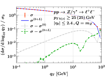
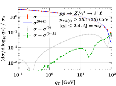
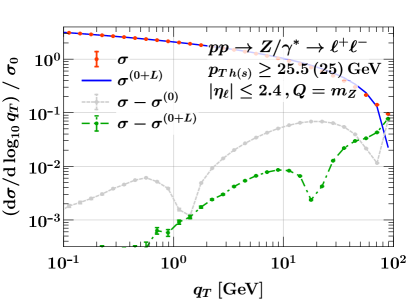
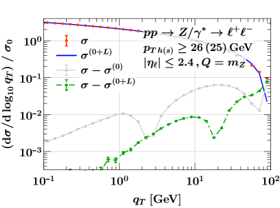
Figure -643: Drell-Yan $q_{T}$ spectrum at fixed $\mathcal{O}(\alpha_{s})$ for different symmetric and slightly asymmetric lepton $p_{T}$ cuts, as indicated in the labels. The full result $\sigma$ is shown by the red points and the LP limit $\sigma^{(0+L)}$ including fiducial power corrections by the blue line. The gray and green curves show the leftover power corrections $\sigma-\sigma^{(0)}$ and $\sigma-\sigma^{(0+L)}$. The error bars indicate the MC integration uncertainties.

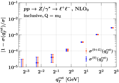
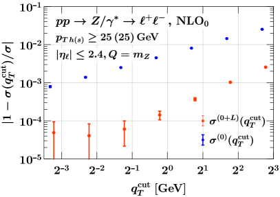
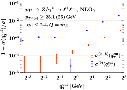
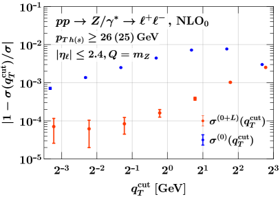
Figure -642: Relative difference between the exact NLO Drell-Yan cross section and its approximation with $q_{T}$ subtractions as a function of $q_{T}^{\mathrm{cut}}$ for different fiducial cuts, as indicated in the labels. The red and blue points correspond to implementing the $q_{T}$ subtraction with $\sigma^{\mathrm{sub}}=\sigma^{(0)}$ and $\sigma^{\mathrm{sub}}=\sigma^{(0+L)}$, respectively. The blue points are slightly shifted for clarity, and the error bars indicate the MC integration uncertainties.

To show the precise effect on the $q_{T}$ subtraction, we show in figure -642 the relative difference between the total cross section obtained via $q_{T}$ subtraction to the reference NLO result obtained from MCFM using Catani-Seymour subtractions as a function of $q_{T}^{\mathrm{cut}}$. The blue points show the result from $q_{T}$ subtractions at strict LP, $\sigma^{\mathrm{sub}}=\sigma^{(0)}$, while the red points show the result including fiducial power corrections in the subtractions, $\sigma^{\mathrm{sub}}=\sigma^{(0+L)}$. The blue points are slightly shifted for better visibility. The uncertainties show the MC integration uncertainties.

For reference, the top-left panel shows the result without any fiducial cuts, in which case there is no difference between the two subtractions. The remaining power corrections are quadratically suppressed, and thus one observes a very good convergence, with deviations to the exact result of only $0.1\%$ already for $q_{T}^{\mathrm{cut}}=3.2\,\mathrm{GeV}$. In the other panels, we show different leptonic cuts. The top-right panel shows the case of equal cuts, $p_{T\,h},p_{T\,s}\geq 25\,\mathrm{GeV}$, while in the bottom we increase the cut on $p_{T\,h}$ to $25.1\,\mathrm{GeV}$ (left) and $26\,\mathrm{GeV}$ (right). (We do not show $p_{T\,h}\geq 25.5\,\mathrm{GeV}$, which does not show any new features.) In all three cases, the power corrections to the subtraction with fiducial power corrections (red points) are of similar size as in the inclusive case. Even though the $q_{T}^{\mathrm{cut}}$ dependence becomes somewhat smaller in magnitude with increasing difference $p_{T\,h}^{\rm min}-p_{T\,s}^{\rm min}$, reflecting a sensitivity on $q_{T}\sim|p_{T\,h}^{\rm min}-p_{T\,s}^{\rm min}|$, this is mostly accounted for by including the fiducial power corrections, and as before choosing $q_{T}^{\mathrm{cut}}\sim 3.2\,\mathrm{GeV}$ suffices for permille accuracy.

In contrast, when implementing the $q_{T}$ subtraction at strict LP (blue points), the size of missing power corrections increases by one to two orders of magnitude, reflecting the enhanced power corrections from the fiducial cuts. To reach the $1\permil$ precision goal requires a substantially smaller $q_{T}^{\mathrm{cut}}\approx 0.1\,\mathrm{GeV}$. Furthermore, we observe again that the shape of the $q_{T}^{\mathrm{cut}}$ dependence of $\sigma^{(0)}(q_{T}^{\mathrm{cut}})$ strongly depends on the precise difference $|p_{T\,h}^{\rm min}-p_{T\,s}^{\rm min}|$ between the lepton cuts. In particular, for $p_{T\,h}\geq 25.1\,\mathrm{GeV}$ (bottom left), we see that the $q_{T}^{\mathrm{cut}}$ dependence accidentally vanishes around $q_{T}^{\mathrm{cut}}=0.8\,\mathrm{GeV}$, while it is quite flat in the region $q_{T}^{\mathrm{cut}}\sim 0.1-0.8\,\mathrm{GeV}$. This region roughly corresponds to the the sign change visible in the corresponding $q_{T}$ spectrum, see figure -643 (top right). This behavior is very dangerous, as it can easily be confused with an apparent convergence if the $q_{T}^{\mathrm{cut}}$ dependence is not properly extrapolated.

In summary, we again find that including the fiducial power corrections in the $q_{T}$ subtraction significantly improves the convergence in the $q_{T}^{\mathrm{cut}}\to 0$ limit, and thus makes the method much more reliable. In particular, for the case of symmetric lepton $p_{T}$ cuts, it recovers the same level of power corrections as for the inclusive case.

6 Comparison to data

In this section, we compare our N³LL$+$NNLO₀ resummed predictions for $q_{T}$ and $\phi^{*}$ for Drell-Yan, $pp\to Z/\gamma^{*}\to\ell^{+}\ell^{-}$ ($\ell=e,\mu)$, with the following precision LHC measurements:

• The ATLAS measurement from ref. [4] using $20.3~{}\,\mathrm{fb}^{-1}$ of 8 TeV data. We consider the $m_{\ell^{+}\ell^{-}}\in[66,116]~{}\,\mathrm{GeV}$ invariant mass bin. The fiducial lepton cuts are $p_{T}>20~{}\,\mathrm{GeV},|\eta|<2.4$ for both electrons and muons. Separate results for the electron and muon channels are reported, in both cases we compare to the measurements using Born leptons. (While the event selection in ref. [4] excludes electrons in the region $1.37<|\eta|<1.52$, this exclusion is removed during the unfolding and not part of the fiducial volume in which the measurements are reported.)

• The CMS measurement from ref. [15] using $35.9~{}\,\mathrm{fb}^{-1}$ of 13 TeV data in the $m_{\ell^{+}\ell^{-}}=m_{Z}\pm 15~{}\,\mathrm{GeV}$ invariant mass bin. The fiducial cuts are given by $p_{T}>25~{}\,\mathrm{GeV}$ and $|\eta|<2.4$ for both electrons and muons. We compare to the combined measurements of dressed electrons and muons.

We consider two sets of predictions: The strict LP resummation with fiducial power corrections only included via the fixed-order matching is denoted as N³LL${}^{(0)}+$NNLO₀, and analogously at lower orders. The resummation including fiducial power corrections is denoted as N³LL${}^{(0+L)}+$NNLO₀, and analogously at lower orders. In this case, the fixed-order matching only adds the remaining genuine (non-fiducial) power corrections.

By default we compare to the measured spectra that are normalized to the total cross section. We correspondingly normalize our predictions to the total fiducial cross section at the corresponding order obtained by integrating the central value for the spectrum to infinity. This effectively amounts to obtaining the total cross section via $q_{T}$ or $\phi^{*}$ subtractions including fiducial power corrections. Since the uncertainties for the total cross section are much smaller than for the spectrum, they are practically irrelevant for this purpose. We have also checked that treating the $\mu_{\mathrm{FO}}$ variation in a correlated fashion or treating it fully uncorrelated between spectrum and normalization and adding it in quadrature leads to essentially identical estimates of the total perturbative uncertainty. For completeness, we also provide analogous comparisons for the unnormalized CMS measurements in appendix B.

6.1 $q_{T}$ spectrum

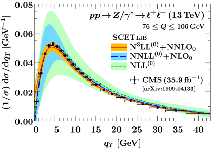
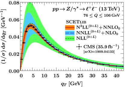
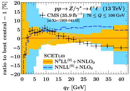
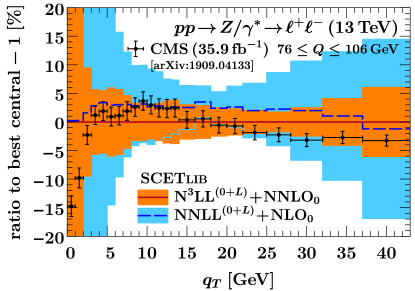
Figure -641: Predictions for the normalized Drell-Yan fiducial $q_{T}$ spectrum without (left) and with (right) resummed fiducial power corrections compared to CMS 13 TeV measurements [15]. The top panels show the spectrum, with the theory predictions drawn as smooth curves for better visibility. The bottom panels show the percent differences to the respective highest-order prediction central value.

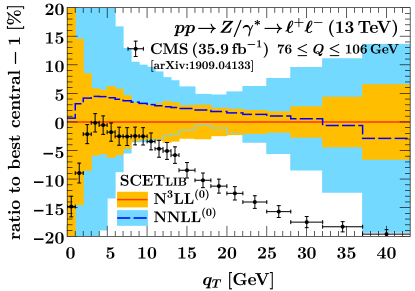
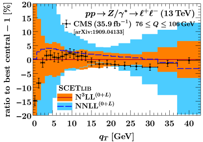
Figure -640: Same as the bottom row of figure -641, but without including power corrections from the fixed-order matching.

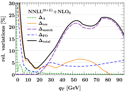
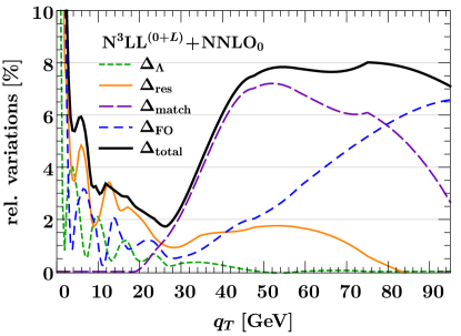
Figure -639: Breakdown of the total uncertainty estimate in the bottom-right panel of figure -641 at NNLL${}^{(0+L)}+$NLO₀ (left) and N³LL${}^{(0+L)}+$NNLO₀ (right). We note the difference in vertical scale. The various contributions are discussed in section 3.4. The total uncertainty estimate (solid black) is obtained by adding the individual contributions in quadrature.

In figure -641, we compare our results to the CMS 13 TeV measurements for $q_{T}$. The top panels show the $q_{T}$ spectrum at NLL (green), NNLL$+$NLO₀ (blue), and N³LL$+$NNLO₀ (orange). The bands show the estimated perturbative uncertainties as discussed in section 3.4. Note that the theory predictions are obtained for the measured binning, but are drawn as smooth curves for clearer visibility. The lower panels show the same results normalized to the respective highest-order prediction. The results using strict LP resummation are shown on the left (lighter shading), while those including the resummation of fiducial power corrections are shown on the right (darker shading). In both cases, we observe good convergence of the resummed predictions, with substantially reduced perturbative uncertainties at subsequent higher orders, as well as good agreement with the data. Nevertheless, resumming the fiducial power corrections on the right further improves the perturbative convergence and also yields a systematically better agreement with the data. The data agreement deteriorates in the first two bins, which can be attributed to small-$q_{T}$ nonperturbative effects. These are expected to become important for $q_{T}\lesssim 2\,\mathrm{GeV}$, but the nonperturbative ingredients necessary to account for these effects are not included in our predictions. This is also reflected in the substantially increased perturbative uncertainties in this region.

A detailed breakdown of our uncertainty estimate is shown in figure -639. As expected, the nonperturbative uncertainty $\Delta_{\Lambda}$ (short-dashed green) only has an impact at low values of $q_{T}\lesssim 10\,\mathrm{GeV}$. The resummation uncertainty $\Delta_{\mathrm{res}}$ (solid orange) dominates up to $q_{T}\approx 30\,\mathrm{GeV}$ at which point the matching uncertainty $\Delta_{\mathrm{match}}$ (long-dashed violet) takes over as the dominant component. The fixed-order uncertainty $\Delta_{\mathrm{FO}}$ (dashed blue) starts to dominate at very high values of $q_{T}\gtrsim 80\,\mathrm{GeV}$ at N³LL$+$NNLO₀, but also has an appreciable impact at low $q_{T}$, where it estimates the fixed-order uncertainties within the resummation. We stress that in the intermediate range $30\leq q_{T}\leq 70\,\mathrm{GeV}$, the $\Delta_{\mathrm{FO}}$ is known to underestimate the perturbative uncertainty in the pure fixed-order results. Supplementing it by the matching uncertainty $\Delta_{\mathrm{match}}$ is thus reasonable as the latter probes a viable set of all-order terms beyond the strict fixed-order result. Note that several of the uncertainty components begin to oscillate strongly for $q_{T}\lesssim 10\,\mathrm{GeV}$. These oscillations are due to the specific implementation of quark flavor thresholds in the PDFs as provided by LHAPDF. The flavor thresholds lead to sharp features in $b_{T}$ space in individual scale variations around $\mu_{B}\sim b_{0}/b_{T}$, which then translate into oscillatory artifacts in $\mathrm{d}\sigma/\mathrm{d}q_{T}$. They are of no concern for the total uncertainty for which they largely average out. It will be interesting to properly address the effect of flavor thresholds in this region along the lines of ref. [89] in the future.

To further illustrate the importance and impact of the fiducial power corrections, in figure -640 we show the analog of the bottom panel of figure -641 but comparing to the pure resummed results, i.e., without including the fixed-order matching corrections to the spectrum. (We still normalize to the same total cross section as in figure -641.) The strict LP resummation (left) completely fails to describe the data, showing that in this case the fixed-order matching corrections that supply the fiducial power corrections at fixed order are essential. On the other hand, upon resumming the fiducial power corrections (right), the excellent data agreement is restored even without the fixed-order matching. In other words, with the fiducial power corrections included in the resummation, the fixed-order matching becomes essentially unimportant for $q_{T}\lesssim 40\,\mathrm{GeV}$, both at NNLL and N³LL.

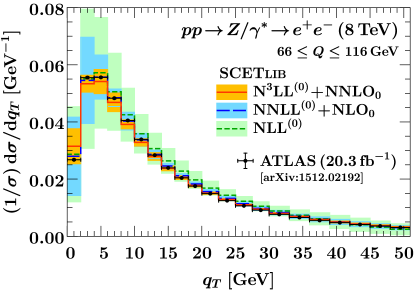
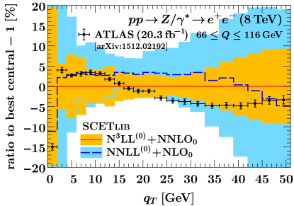
Figure -638: Predictions for the normalized Drell-Yan fiducial $q_{T}$ spectrum without (left) and with (right) resummed fiducial power corrections compared to ATLAS 8 TeV measurements [4] in the $e^{+}e^{-}$ channel. The top panels show the normalized spectrum. The bottom panels show the percent differences to the respective highest-order prediction central value. The analogous results for the $\mu^{+}\mu^{-}$ channel can be seen in appendix B in figure -632.

In figure -638, we show the analogous comparison for the ATLAS 8 TeV measurements [4] in the electron channel, with the top panel showing the $q_{T}$ spectrum itself, while the bottom panel shows the relative differences to the respective highest-order prediction. As before, we see good perturbative convergence of the predictions, as well as good agreement with the data. The data agreement again improves when resumming the fiducial power corrections on the right, leading to an overall flatter shape and reduced size in the difference between predictions and measurement. The results in the muon channel are practically identical, and are provided for completeness in figure -632 in appendix B.

6.2 $\phi^{*}$ distribution

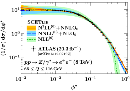
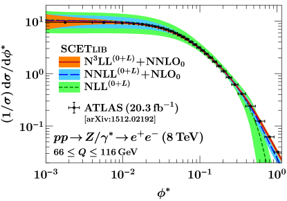
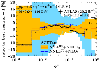
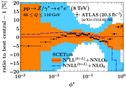
Figure -637: Predictions for the normalized Drell-Yan fiducial $\phi^{*}$ spectrum using the LP resummation (left) and including the resummation of fiducial power corrections (right) compared to ATLAS 8 TeV measurements [4] in the $e^{+}e^{-}$ channel. The top panels show the spectrum, with the predictions drawn as smooth curves for better visibility. The bottom panels show the percent differences to the respective highest-order prediction central value. The analogous result for the $\mu^{+}\mu^{-}$ channel can be seen in appendix B in figure -631.

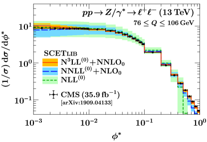
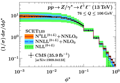
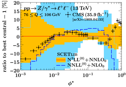
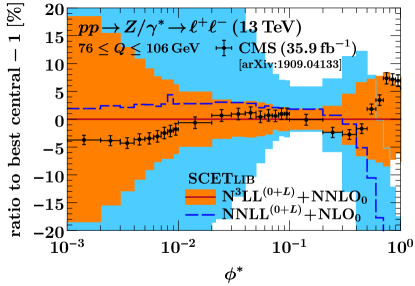
Figure -636: Predictions for the normalized Drell-Yan fiducial $\phi^{*}$ spectrum using the LP resummation (left) and including the resummation of fiducial power corrections (right) compared to CMS 13 TeV measurements [15]. The top panels show the spectrum, and the bottom panels show the percent differences to the respective highest-order prediction central value.

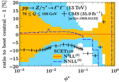
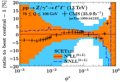
Figure -635: Same as the bottom row of figure -636, but without including power corrections from the fixed-order matching.

In figure -637, we compare our results for the $\phi^{*}$ spectrum to the ATLAS 8 TeV measurements [4] in the electron channel. The analogous results in the muon channel are provided in appendix B in figure -631. The top panel shows the predictions at NLL (green), NNLL$+$NLO₀ (blue), and N³LL$+$NNLO₀ (orange), with the bands showing the estimated perturbative uncertainties as discussed in section 3.4. The predictions are obtained with the experimental binning but are drawn as smooth curves for better visibility. The lower panels show the same results normalized to the respective highest-order predictions. The results using strict LP resummation for both the observable itself and the fiducial cuts are shown on the left (lighter shading), while those including the resummation of fiducial power corrections for observable and cuts are shown on the right (darker shading). In both cases we observe good convergence of the resummed predictions. For large $\phi^{*}\gtrsim 0.5$, the spectrum enters the fixed-order region and consequently the NLL (green) results start to deviate substantially, and to lesser extent also the NNLL$+$NLO₀ (blue) results. The first one or two bins are again sensitive to small-$q_{T}$ nonperturbative effects, which is reflected in their increased perturbative uncertainties. As for the $q_{T}$ spectrum, we find excellent agreement with the data, which is further improved on the right by resumming the fiducial power corrections, especially at NNLL$+$NLO₀ where the shape improves significantly.

In figure -636, we show the analogous comparison for the CMS 13 TeV $\phi^{*}$ measurements [15]. The top panels show the spectrum itself, and the bottom panels the relative difference to the respective highest-order prediction. The predictions show the same behaviour as at 8 TeV, and we again find good agreement with the data. Here, the improvements from resumming the fiducial power corrections are even more striking. While the strict LP resummation on the left shows a clear trend of overshooting the data at small $\phi^{*}$, we find nigh-perfect agreement across the spectrum with resummed fiducial power corrections. To further highlight this, in figure -635 we show the analog of the bottom panel of figure -636 but comparing to the pure resummed results only, i.e., without including fixed-order matching corrections. As we already saw for the $q_{T}$ spectrum, the LP resummation alone (left) basically fails to describe the data, showing that in this case the fixed-order matching is necessary in order to supply the fiducial power corrections at least at fixed order. In contrast, when resumming the fiducial power corrections (right), we find the same excellent data agreement as before up to $\phi^{*}\lesssim 0.5$. This shows that the $\phi^{*}$ spectrum has rather large sensitivity to power corrections throughout its spectrum and profits enormously from including them in the resummation. At the same time, the remaining fixed-order power corrections become almost negligible in this range. Beyond $\phi^{*}\gtrsim 0.5$, we enter the fixed-order region and as expected, the pure resummed results quickly deteriorate and matching to the fixed-order results becomes strictly necessary.

7 Conclusions

We have studied the impact of fiducial cuts and other generic leptonic measurements on the factorization of the Drell-Yan process at small transverse momentum $q_{T}\ll Q$. They generically induce fiducial power corrections in $q_{T}/Q$ relative to the well-studied leading-power terms predicted by $q_{T}$ (equivalently TMD) factorization, which are significantly larger than the quadratic power corrections arising for the inclusive $q_{T}$ spectrum.

Using a Lorentz-covariant tensor decomposition of the leptonic and hadronic tensors combined with formal power-counting arguments in SCET, we have shown that for a large class of observables (those that are azimuthally symmetric at leading power), the fiducial power corrections are the only source of linear power corrections. Furthermore, by retaining the exact leptonic structure functions, the fiducial power corrections are unambiguously predicted from factorization and are correctly resummed to the same order as the leading-power corrections.

We have also shown that the naive power expansion in $q_{T}/Q\ll 1$ can break down near the edge of Born phase space due to uncontrolled leptonic power corrections $\sim q_{T}/p_{L}$, where $p_{L}$ is the distance from the edge of Born phase space. In such regions, it is strictly required to keep all leptonic power corrections $\sim q_{T}/p_{L}$ to correctly describe the actual leading-power limit. An important example is the $p_{T}^{\ell}$ spectrum near the Jacobian peak $p_{T}^{\ell}=Q/2$ with $p_{L}=Q-2p_{T}^{\ell}$. This provides another formal reason to keep the exact leptonic structure functions, because doing so guarantees that all required leptonic power corrections are automatically retained. The kinematic recoil prescriptions used in practical implementations usually yield an exact description of the leptonic decay and measurements. Our analysis shows for the first time that this is not only justified, but even necessary to obtain a description that is formally valid across the entire leptonic phase space. These conclusions also immediately apply to scalar processes such as Higgs production.

The tensor decomposition can be interpreted as a specific choice of vector-boson rest frame, which naturally emerged to be the Collins-Soper frame as defined by boosting from the lab frame, even when keeping nonzero masses of the initial state hadrons. The CS tensor decomposition yields nine Lorentz-scalar hadronic structure functions, which are defined for an arbitrary leptonic final state, and for $Z/\gamma^{*}\to\ell\ell$ or $W\to\ell\nu$ decays directly map onto the commonly used angular coefficients for the cross section in the CS angles. We also discussed that Born leptons can be theoretically well defined in terms of an IR-safe Born projection of the full leptonic final state, including QED final-state radiation. We have shown that the cross section in the CS angles of the so-defined Born leptons admits a LO-like complete angular decomposition in terms of spherical harmonics, with the corresponding generalized angular coefficients modified by QED corrections.

We have presented resummed predictions with and without the resummation of fiducial power corrections at N³LL. The comparison of our predictions to precision Drell-Yan $q_{T}$ and $\phi^{*}$ measurements from ATLAS and CMS confirms the importance of fiducial power corrections and their resummation in a striking way: While the strict LP resummation is able to describe the data within (theory) uncertainties, it fails to do so without including the sizeable fixed-order corrections. On the other hand, including the fiducial power corrections in the resummation systematically improves the agreement with the data, particularly at very small $q_{T}$ and $\phi^{*}$. Furthermore, the fixed-order matching corrections now become very small and do not play much of a role below $q_{T}\lesssim 40\,\mathrm{GeV}$ and $\phi^{*}\lesssim 0.5$. Since the importance of unresummed, fixed-order power corrections is significantly reduced by resumming the fiducial power corrections, this has important implications for all phenomenological applications at small $q_{T}$, for example the extraction of nonperturbative inputs to TMD distributions from data.

Furthermore, it is also much cheaper computationally to predict or obtain the fiducial power corrections via factorization instead of including (or extracting) them numerically from the full fixed-order calculations, since the latter become expensive quickly toward small $q_{T}$ or may not even be available. This is also reflected in a significantly improved performance for the $q_{T}$ subtraction method when the fiducial power corrections are included in the subtraction term predicted from factorization. In particular, this extends the applicability of the subtraction method to phase-space regions where it would otherwise break down due to uncontrolled leptonic power corrections. We have explicitly demonstrated this numerically for the $p_{T}^{\ell}$ spectrum near the Jacobian edge $p_{T}^{\ell}=m_{W}/2$. As a second example, we have studied the $q_{T}$ subtraction for Drell-Yan production with symmetric cuts on the final-state leptons, where we observed that enhanced power corrections from choosing symmetric cuts are fully accounted for by our formalism.

We have also considered the resummed $p_{T}^{\ell}$ spectrum, which plays a crucial role in the precision $m_{W}$ measurement at the LHC, and have obtained the first N³LL predictions for it. We have demonstrated that a reliable prediction of the physical $p_{T}^{\ell}$ spectrum near the Jacobian peak is possible and that it relies in an essential way on the interplay between small-$q_{T}$ resummation effects and the exact treatment of leptonic power corrections that describe the recoil of the leptonic system. The effective enhancement from leptonic power corrections also induces an enhanced sensitivity to additional hadronic structure functions. We stress that these effects are suppressed in the $q_{T}$ spectrum itself, where they only enter indirectly through fiducial cuts. In contrast, they are directly exposed in the $p_{T}^{\ell}$ spectrum near the Jacobian peak. We therefore encourage precise, unfolded measurements of the $p_{T}^{\ell}$ spectrum for both $W$ and $Z$ in this region. Other interesting measurements would be the double-differential spectrum in the lepton momenta $p_{T1},p_{T2}$, or equivalently $p_{T1}\pm p_{T2}$, which can be expected to provide further sensitivity to these effects.

Appendix A Hard functions and leptonic tensors for Drell-Yan

A.1 Hard functions

At leading power in $\lambda$, the hard contribution to the hadronic tensor in the limit $\lambda\ll 1$ is given by [147],

$$H_{VV^{\prime}\,q{\bar{q}}^{\prime}}^{\mu\nu}(n_{a},n_{b};\omega_{a},\omega_{b}) =2\frac{1}{4N_{c}}\operatorname{tr}\Bigl{[}\frac{\not{n}_{a}}{2}{\bar{C}}^{(0)\mu}_{V\,q{\bar{q}}^{\prime}}(n_{b},n_{a};\omega_{b},\omega_{a})\frac{\not{n}_{b}}{2}C^{(0)\nu}_{V^{\prime}\,q{\bar{q}}^{\prime}}(n_{b},n_{a};\omega_{b},\omega_{a})\Bigr{]}$$

$$\quad+\Bigl{(}\text{terms}\,\propto\operatorname{tr}\Bigl{[}\not{n}_{a}\not{n}_{\perp a}{\bar{C}}^{(0)\mu}_{V\,q{\bar{q}}^{\prime}}\,\not{n}_{\perp b}\not{n}_{b}\,C^{(0)\nu}_{V^{\prime}\,q{\bar{q}}^{\prime}}\Bigr{]}\Bigr{)}\,,$$ (A.1)

where $C^{{(0)}\mu\,\alpha\beta}_{V,q{\bar{q}}^{\prime}}$ are the hard matching coefficients in eq. (2.6.1), ${\bar{C}}^{\mu\beta\alpha}=[\gamma^{0}C^{\dagger\mu}\gamma^{0}]^{\beta\alpha}$, and the trace is over the Dirac indices. The additional terms in parenthesis in the second line do not contribute to $H_{-1,4}$ but only to $H_{2,5}$ relevant for the Boer-Mulders effect, see eq. (2.103), where the $n_{\perp a,b}$ are transverse unit vectors associated with the Boer-Mulders functions $h_{1a,b}^{\perp}$.

We remind the reader that the $VV^{\prime}$ indices were largely left implicit in the main text. Using eq. (2.3.2), the hard functions $H_{i\,VV^{\prime}\,q{\bar{q}}^{\prime}}$ for $i=-1,4$ are given by the projections onto $x_{\mu}x_{\nu}+y_{\mu}y_{\nu}=-g_{\perp\mu\nu}+\mathcal{O}(\lambda)$ and $2\mathrm{i}\bigl{(}x_{\mu}y_{\nu}-x_{\nu}y_{\mu}\bigr{)}=2\mathrm{i}\epsilon_{\perp\mu\nu}+\mathcal{O}(\lambda)$,

$$H_{-1\,VV^{\prime}\,q{\bar{q}}^{\prime}}(q^{2})=-g_{\perp\mu\nu}H_{VV^{\prime}\,q{\bar{q}}^{\prime}}^{\mu\nu}(n_{a},n_{b};\omega_{a},\omega_{b})\,,$$

$$H_{4\,VV^{\prime}\,q{\bar{q}}^{\prime}}(q^{2})=2\mathrm{i}\epsilon_{\perp\mu\nu}H_{VV^{\prime}\,q{\bar{q}}^{\prime}}^{\mu\nu}(n_{a},n_{b};\omega_{a},\omega_{b})\,.$$ (A.2)

Here we used that the projected hard function can only depend on the Lorentz scalar $q^{2}=\omega_{a}\omega_{b}$.

The case of an incoming antiquark in the $a$ direction follows from $a\leftrightarrow b$,

$$H_{VV^{\prime}\,{\bar{q}}^{\prime}q}^{\mu\nu}(n_{a},n_{b};\omega_{a},\omega_{b})=H_{VV^{\prime}\,q{\bar{q}}^{\prime}}^{\mu\nu}(n_{b},n_{a};\omega_{b},\omega_{a})\,.$$ (A.3)

This implies

$$H_{-1\,VV^{\prime}\,{\bar{q}}^{\prime}q}(q^{2})=+H_{-1\,VV^{\prime}\,q{\bar{q}}^{\prime}}(q^{2})\,,\qquad H_{4\,VV^{\prime}\,{\bar{q}}^{\prime}q}(q^{2})=-H_{4\,VV^{\prime}\,q{\bar{q}}^{\prime}}(q^{2})\,,$$ (A.4)

as expected from parity. In the inclusive case discussed in section 2.2, we used the shorthand

$$H_{VV^{\prime}\,ab}(q^{2})\equiv H_{-1\,VV^{\prime}\,ab}(q^{2})\,.$$ (A.5)

Inserting the expression in eq. (2.6.1) into eq. (A.1), and suppressing the $q^{2}$ argument for brevity, we find

$$H_{-1\,ZZ\,q{\bar{q}}^{\prime}} =\frac{8\pi\alpha_{\mathrm{em}}}{N_{c}}\delta_{qq^{\prime}}\Bigl{\{}(v_{q}^{2}+a_{q}^{2})\lvert C_{q}\rvert^{2}+2\Re\sum_{f}\bigl{(}v_{q}v_{f}C_{q}^{*}C_{vf}+a_{q}a_{f}C_{q}^{*}C_{af}\bigr{)}+\mathcal{O}(\alpha_{s}^{4})\Bigr{\}}\,,$$

$$H_{-1\,\gamma\gamma\,q{\bar{q}}^{\prime}} =\frac{8\pi\alpha_{\mathrm{em}}}{N_{c}}\delta_{qq^{\prime}}\Bigl{\{}Q_{q}^{2}\lvert C_{q}\rvert^{2}+2\Re\sum_{f}Q_{q}Q_{f}C_{q}^{*}C_{vf}+\mathcal{O}(\alpha_{s}^{6})\Bigr{\}}\,,$$

$$H_{-1\,Z\gamma\,q{\bar{q}}^{\prime}} =\frac{8\pi\alpha_{\mathrm{em}}}{N_{c}}\delta_{qq^{\prime}}\Bigl{\{}-v_{q}Q_{q}\lvert C_{q}\rvert^{2}-\sum_{f}\bigl{(}v_{f}Q_{q}C_{vf}^{*}C_{q}+v_{q}Q_{f}C_{q}^{*}C_{vf}\bigr{)}+\mathcal{O}(\alpha_{s}^{6})\Bigr{\}}$$

$$=H^{*}_{-1\,\gamma Z\,q{\bar{q}}^{\prime}}\,,$$ (A.6)

where $\Re$ denotes the real part, the vector ($v_{f}$) and axial ($a_{f}$) couplings of a quark of flavor $f$ to the $Z$ boson were given in eq. (2.3). The terms denoted as $\mathcal{O}(\alpha_{s}^{4,6})$ are proportional to the square of the singlet matching coefficients, which only start at $C_{af}=\mathcal{O}(\alpha_{s}^{2})$ and $C_{vf}=\mathcal{O}(\alpha_{s}^{3})$, whereas the nonsinglet coefficient $C_{q}=1+\mathcal{O}(\alpha_{s})$. In the parity-odd case, we have

$$H_{4\,ZZ\,q{\bar{q}}^{\prime}} =\frac{16\pi\alpha_{\mathrm{em}}}{N_{c}}\delta_{qq^{\prime}}\Bigl{\{}2v_{q}a_{q}\lvert C_{q}\rvert^{2}+2\Re\sum_{f}\bigl{(}v_{q}a_{f}C_{q}^{*}C_{af}+a_{q}v_{f}C_{q}^{*}C_{vf}\bigr{)}+\mathcal{O}(\alpha_{s}^{5})\Bigr{\}}\,,$$

$$H_{4\,\gamma\gamma\,q{\bar{q}}^{\prime}} =0\,,$$

$$H_{4\,Z\gamma\,q{\bar{q}}^{\prime}} =\frac{16\pi\alpha_{\mathrm{em}}}{N_{c}}\delta_{qq^{\prime}}\Bigl{\{}-a_{q}Q_{q}\lvert C_{q}\rvert^{2}-\sum_{f}\bigl{(}a_{f}Q_{q}C_{af}^{*}C_{q}+a_{q}Q_{f}C_{q}^{*}C_{vf}\bigr{)}+\mathcal{O}(\alpha_{s}^{5})\Bigr{\}}$$

$$=H^{*}_{4\,\gamma Z\,q{\bar{q}}^{\prime}}\,.$$ (A.7)

For $W^{\pm}$ exchange, we have

$$H_{-1\,W^{+}W^{+}\,q{\bar{q}}^{\prime}} =\frac{2\pi\alpha_{\mathrm{em}}}{N_{c}}\frac{\lvert V_{qq^{\prime}}\rvert^{2}}{\sin^{2}\theta_{w}}\lvert C_{q}\rvert^{2}\,,\qquad H_{4\,W^{+}W^{+}\,q{\bar{q}}^{\prime}}=\frac{4\pi\alpha_{\mathrm{em}}}{N_{c}}\frac{\lvert V_{qq^{\prime}}\rvert^{2}}{\sin^{2}\theta_{w}}\lvert C_{q}\rvert^{2}\,,$$

$$H_{-1\,W^{-}W^{-}\,q{\bar{q}}^{\prime}} =\frac{2\pi\alpha_{\mathrm{em}}}{N_{c}}\frac{\lvert V_{q^{\prime}q}\rvert^{2}}{\sin^{2}\theta_{w}}\lvert C_{q}\rvert^{2}\,,\qquad H_{4\,W^{-}W^{-}\,q{\bar{q}}^{\prime}}=\frac{4\pi\alpha_{\mathrm{em}}}{N_{c}}\frac{\lvert V_{q^{\prime}q}\rvert^{2}}{\sin^{2}\theta_{w}}\lvert C_{q}\rvert^{2}\,,$$ (A.8)

where $V_{qq^{\prime}}$ denotes the CKM-matrix element for $q\in\{u,c,t\}$ and $q^{\prime}\in\{d,s,b\}$ (and we take it to vanish in all other cases). The overall relative factor of $2$ between $H_{-1}$ and $H_{4}$ is due to the conventional normalization of $g_{4}(\theta,\varphi)=\cos\theta$ rather than $2\cos\theta$ in eq. (2.4.2).

The renormalized matching coefficients $C_{q}(q^{2},\mu)$ and $C_{vf,af}(q^{2},\mu)$ can be extracted from the IR-finite parts of the $q\bar{q}$ vector and axial-vector form factors, which admit the same flavor decomposition as eq. (2.6.1). Explicit expressions for $C_{q}(q^{2},\mu)$ in our notation can be found in ref. [183]. The two-loop results which enter in our analysis follow from the two-loop quark form factors [215, 216, 217, 218]. In principle, there is an $\mathcal{O}(\alpha_{s}^{2})$ contribution to the axial-vector singlet coefficient if the top quark is taken to be massive at the hard scale [147]. These contributions have however been found to be small at the level of the total cross section [123, 17], and we neglect them in this paper.

A.2 Leptonic tensors

The leptonic scalar coefficients $L_{\pm\,VV^{\prime}}(q^{2})$ defined in eq. (2.58) encode the squared electroweak decay matrix element including the vector-boson propagator. In the inclusive case discussed in section 2.2, we used the shorthand

$$L(q^{2})\equiv L_{+\,VV^{\prime}}(q^{2})\,.$$ (A.9)

For $Z/\gamma^{*}\to\ell^{+}\ell^{-}$, the parity-even leptonic coefficients read

$$L_{+\,ZZ}(q^{2}) =\frac{2}{3}\frac{\alpha_{\mathrm{em}}}{q^{2}}\,(v_{\ell}^{2}+a_{\ell}^{2})\,\bigl{\lvert}P_{Z}(q^{2})\bigr{\rvert}^{2}\,,\qquad L_{+\,\gamma\gamma}(q^{2}) =\frac{2}{3}\frac{\alpha_{\mathrm{em}}}{q^{2}}\,Q_{\ell}^{2}\,,$$

$$L_{+\,\gamma Z}(q^{2}) =\frac{2}{3}\frac{\alpha_{\mathrm{em}}}{q^{2}}\,(-v_{\ell}\,Q_{\ell})\,P_{Z}(q^{2})\,,\qquad L_{+\,Z\gamma}(q^{2}) =L_{+\,\gamma Z}^{*}(q^{2})\,.$$ (A.10)

The parity-odd coefficients arise from the interference of axial and vector current contributions,

$$L_{-\,ZZ}(q^{2}) =\frac{2}{3}\frac{\alpha_{\mathrm{em}}}{q^{2}}\,(2v_{\ell}\,a_{\ell})\,\bigl{\lvert}P_{Z}(q^{2})\bigr{\rvert}^{2}\,,\qquad L_{-\,\gamma\gamma}(q^{2}) =0\,,$$

$$L_{-\,\gamma Z}(q^{2}) =\frac{2}{3}\frac{\alpha_{\mathrm{em}}}{q^{2}}\,(-a_{\ell}Q_{\ell})\,P_{Z}(q^{2})\,,\qquad L_{-\,Z\gamma}(q^{2}) =L_{-\,\gamma Z}^{*}(q^{2})\,.$$ (A.11)

Here, $Q_{\ell}=-1$, and the vector ($v_{\ell}$) and axial couplings ($a_{\ell}$) of the lepton $\ell$ to the $Z$ boson have the same form as eq. (2.3) with $T_{3}^{\ell}=-1/2$. The $Z\to\nu\bar{\nu}$ process is obtained by the replacement $\ell\to\nu$ with $Q_{\nu}=0$ and $T_{3}^{\nu}=+1/2$. The reduced propagator $P_{V}$ is given by

$$P_{V}(q^{2})=\frac{q^{2}}{q^{2}-m_{V}^{2}+\mathrm{i}\Gamma_{V}m_{V}}\,.$$ (A.12)

For $W\to\ell\nu$, the $L_{\pm}(q^{2})$ are equal due to the current’s $V-A$ structure, and are given by

$$L_{+\,W^{\pm}W^{\pm}}(q^{2})=L_{-\,W^{\pm}W^{\pm}}(q^{2})=\frac{1}{6}\frac{\alpha_{\mathrm{em}}}{q^{2}}\,\frac{1}{\sin^{2}\theta_{w}}\,\bigl{\lvert}P_{W}(q^{2})\bigr{\rvert}^{2}\,.$$ (A.13)

Appendix B Additional comparisons to data

B.1 Unnormalized results

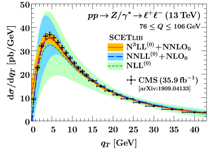
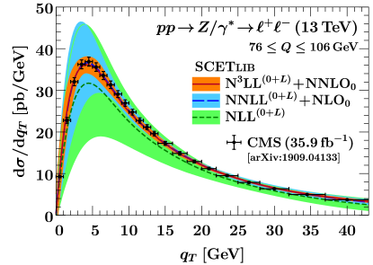
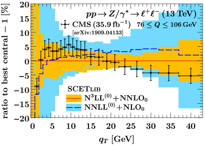
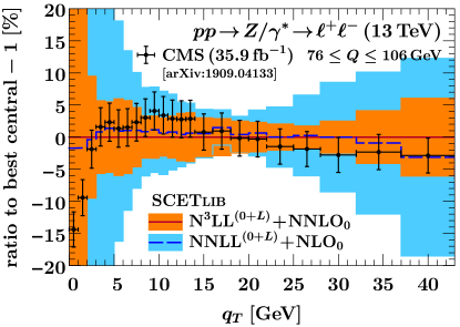
Figure -634: Comparison to CMS $13\,\mathrm{TeV}$ measurements [15] analogous to figure -641 but for the unnormalized, absolute $q_{T}$ spectrum.

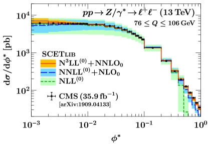
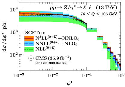
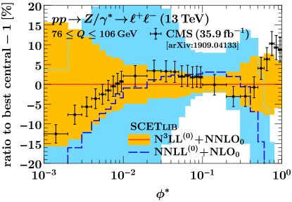
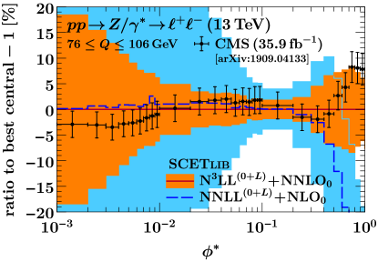
Figure -633: Comparison to CMS $13\,\mathrm{TeV}$ measurements [15] analogous to figure -636 but for the unnormalized, absolute $\phi^{*}$ spectrum.

In section 6, we compared our predictions to the CMS $13\,\mathrm{TeV}$ measurements from ref. [15] using the normalized $q_{T}$ and $\phi^{*}$ spectra. For completeness, here we show the corresponding results for the unnormalized, absolute $q_{T}$ spectrum in figure -634 and $\phi^{*}$ spectrum in figure -633. The experimental uncertainties are larger for the absolute spectra than the normalized ones but include a substantial correlated component from the overall absolute normalization of the measurement. The absolute spectra show the same systematic improvement in the predictions from resumming the fiducial power corrections.

B.2 Results for $\mu^{+}\mu^{-}$ channel

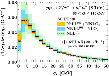
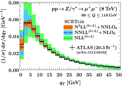
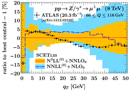
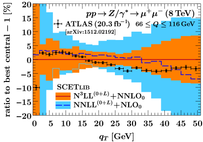
Figure -632: Comparison to ATLAS $8\,\mathrm{TeV}$ $q_{T}$ measurements [4] in the $\mu^{+}\mu^{-}$ channel, analogous to the $e^{+}e^{-}$ channel in figure -638.

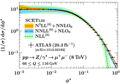
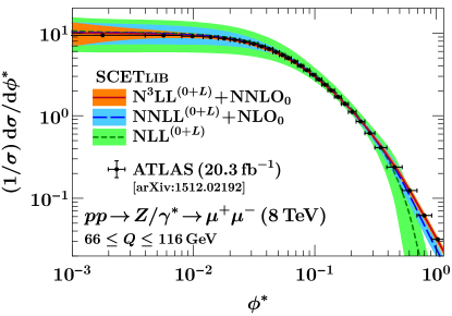
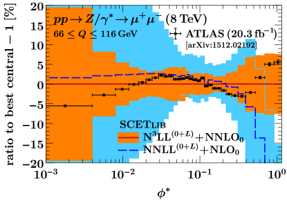
Figure -631: Comparison to ATLAS $8\,\mathrm{TeV}$ $\phi^{*}$ measurements [4] in the $\mu^{+}\mu^{-}$ channel, analogous to the $e^{+}e^{-}$ channel in figure -637.

In section 6, we compared our predictions to the ATLAS $8\,\mathrm{TeV}$ measurements [4] in the $pp\to Z/\gamma^{*}\to e^{+}e^{-}$ channel. For completeness, here we compare the same predictions to the data taken in the $pp\to Z/\gamma^{*}\to\mu^{+}\mu^{-}$ channel. In figure -632, we compare to the measurement of the $q_{T}$ spectrum in the muon channel, which corresponds to figure -638 in the electron channel. In figure -631, we show the results for the $\phi^{*}$ spectrum in the muon channel, which corresponds to figure -637 in the electron channel. The muon data follow the same trends and confirm the conclusions drawn in section 6.

References

- [1] ATLAS collaboration, Measurement of angular correlations in Drell-Yan lepton pairs to probe Z/gamma* boson transverse momentum at sqrt(s)=7 TeV with the ATLAS detector, Phys. Lett. B 720 (2013) 32 [1211.6899].
- [2] ATLAS collaboration, Measurement of the boson transverse momentum distribution in collisions at = 7 TeV with the ATLAS detector, JHEP 09 (2014) 145 [1406.3660].
- [3] ATLAS collaboration, Measurement of the forward-backward asymmetry of electron and muon pair-production in collisions at = 7 TeV with the ATLAS detector, JHEP 09 (2015) 049 [1503.03709].
- [4] ATLAS collaboration, Measurement of the transverse momentum and distributions of Drell-Yan lepton pairs in proton-proton collisions at TeV with the ATLAS detector, Eur. Phys. J. C76 (2016) 291 [1512.02192].
- [5] ATLAS collaboration, Measurement of the angular coefficients in -boson events using electron and muon pairs from data taken at TeV with the ATLAS detector, JHEP 08 (2016) 159 [1606.00689].
- [6] ATLAS collaboration, Measurement of the Drell-Yan triple-differential cross section in collisions at TeV, JHEP 12 (2017) 059 [1710.05167].
- [7] ATLAS collaboration, Measurement of the -boson mass in pp collisions at TeV with the ATLAS detector, Eur. Phys. J. C78 (2018) 110 [1701.07240].
- [8] ATLAS collaboration, Measurement of the transverse momentum distribution of Drell-Yan lepton pairs in proton-proton collisions at TeV with the ATLAS detector, Eur. Phys. J. C 80 (2020) 616 [1912.02844].
- [9] CMS collaboration, Measurement of the Rapidity and Transverse Momentum Distributions of Bosons in Collisions at TeV, Phys. Rev. D 85 (2012) 032002 [1110.4973].
- [10] CMS collaboration, Measurement of the Z boson differential cross section in transverse momentum and rapidity in proton–proton collisions at 8 TeV, Phys. Lett. B 749 (2015) 187 [1504.03511].
- [11] CMS collaboration, Angular coefficients of Z bosons produced in pp collisions at = 8 TeV and decaying to as a function of transverse momentum and rapidity, Phys. Lett. B 750 (2015) 154 [1504.03512].
- [12] CMS collaboration, Measurement of the transverse momentum spectra of weak vector bosons produced in proton-proton collisions at TeV, JHEP 02 (2017) 096 [1606.05864].
- [13] CMS collaboration, Measurement of differential cross sections in the kinematic angular variable for inclusive Z boson production in pp collisions at 8 TeV, JHEP 03 (2018) 172 [1710.07955].
- [14] CMS collaboration, Measurement of the weak mixing angle using the forward-backward asymmetry of Drell-Yan events in pp collisions at 8 TeV, Eur. Phys. J. C78 (2018) 701 [1806.00863].
- [15] CMS collaboration, Measurements of differential Z boson production cross sections in proton-proton collisions at 13 TeV, JHEP 12 (2019) 061 [1909.04133].
- [16] G. Altarelli, R. Ellis and G. Martinelli, Large Perturbative Corrections to the Drell-Yan Process in QCD, Nucl. Phys. B 157 (1979) 461.
- [17] R. Hamberg, W. van Neerven and T. Matsuura, A complete calculation of the order correction to the Drell-Yan factor, Nucl. Phys. B 359 (1991) 343.
- [18] W. van Neerven and E. Zijlstra, The corrected Drell-Yan factor in the DIS and MS scheme, Nucl. Phys. B 382 (1992) 11.
- [19] R. V. Harlander and W. B. Kilgore, Next-to-next-to-leading order Higgs production at hadron colliders, Phys. Rev. Lett. 88 (2002) 201801 [hep-ph/0201206].
- [20] C. Anastasiou, L. J. Dixon, K. Melnikov and F. Petriello, Dilepton rapidity distribution in the Drell-Yan process at NNLO in QCD, Phys. Rev. Lett. 91 (2003) 182002 [hep-ph/0306192].
- [21] C. Anastasiou, L. J. Dixon, K. Melnikov and F. Petriello, High precision QCD at hadron colliders: Electroweak gauge boson rapidity distributions at NNLO, Phys. Rev. D 69 (2004) 094008 [hep-ph/0312266].
- [22] K. Melnikov and F. Petriello, The boson production cross section at the LHC through , Phys. Rev. Lett. 96 (2006) 231803 [hep-ph/0603182].
- [23] K. Melnikov and F. Petriello, Electroweak gauge boson production at hadron colliders through , Phys. Rev. D 74 (2006) 114017 [hep-ph/0609070].
- [24] S. Catani, L. Cieri, G. Ferrera, D. de Florian and M. Grazzini, Vector boson production at hadron colliders: a fully exclusive QCD calculation at NNLO, Phys. Rev. Lett. 103 (2009) 082001 [0903.2120].
- [25] R. Gavin, Y. Li, F. Petriello and S. Quackenbush, FEWZ 2.0: A code for hadronic Z production at next-to-next-to-leading order, Comput. Phys. Commun. 182 (2011) 2388 [1011.3540].
- [26] R. Gavin, Y. Li, F. Petriello and S. Quackenbush, W Physics at the LHC with FEWZ 2.1, Comput. Phys. Commun. 184 (2013) 208 [1201.5896].
- [27] S. Höche, Y. Li and S. Prestel, Drell-Yan lepton pair production at NNLO QCD with parton showers, Phys. Rev. D 91 (2015) 074015 [1405.3607].
- [28] A. Karlberg, E. Re and G. Zanderighi, NNLOPS accurate Drell-Yan production, JHEP 09 (2014) 134 [1407.2940].
- [29] S. Alioli, C. W. Bauer, C. Berggren, F. J. Tackmann and J. R. Walsh, Drell-Yan production at NNLLNNLO matched to parton showers, Phys. Rev. D 92 (2015) 094020 [1508.01475].
- [30] S. Moch and A. Vogt, Higher-order soft corrections to lepton pair and Higgs boson production, Phys. Lett. B 631 (2005) 48 [hep-ph/0508265].
- [31] V. Ravindran, J. Smith and W. van Neerven, QCD threshold corrections to di-lepton and Higgs rapidity distributions beyond LO, Nucl. Phys. B 767 (2007) 100 [hep-ph/0608308].
- [32] T. Ahmed, M. Mahakhud, N. Rana and V. Ravindran, Drell-Yan Production at Threshold to Third Order in QCD, Phys. Rev. Lett. 113 (2014) 112002 [1404.0366].
- [33] Y. Li, A. von Manteuffel, R. M. Schabinger and H. X. Zhu, N3LO Higgs boson and Drell-Yan production at threshold: The one-loop two-emission contribution, Phys. Rev. D 90 (2014) 053006 [1404.5839].
- [34] T. Ahmed, M. K. Mandal, N. Rana and V. Ravindran, Rapidity Distributions in Drell-Yan and Higgs Productions at Threshold to Third Order in QCD, Phys. Rev. Lett. 113 (2014) 212003 [1404.6504].
- [35] S. Catani, L. Cieri, D. de Florian, G. Ferrera and M. Grazzini, Threshold resummation at N3LL accuracy and soft-virtual cross sections at N3LO, Nucl. Phys. B 888 (2014) 75 [1405.4827].
- [36] G. Lustermans, J. K. Michel and F. J. Tackmann, Generalized Threshold Factorization with Full Collinear Dynamics, 1908.00985.
- [37] C. Duhr, F. Dulat and B. Mistlberger, Drell-Yan Cross Section to Third Order in the Strong Coupling Constant, Phys. Rev. Lett. 125 (2020) 172001 [2001.07717].
- [38] U. Baur, S. Keller and W. K. Sakumoto, QED radiative corrections to boson production and the forward backward asymmetry at hadron colliders, Phys. Rev. D57 (1998) 199 [hep-ph/9707301].
- [39] U. Baur, S. Keller and D. Wackeroth, Electroweak radiative corrections to boson production in hadronic collisions, Phys. Rev. D59 (1999) 013002 [hep-ph/9807417].
- [40] U. Baur, O. Brein, W. Hollik, C. Schappacher and D. Wackeroth, Electroweak radiative corrections to neutral current Drell-Yan processes at hadron colliders, Phys. Rev. D65 (2002) 033007 [hep-ph/0108274].
- [41] S. Dittmaier and M. Krämer, Electroweak radiative corrections to W boson production at hadron colliders, Phys. Rev. D65 (2002) 073007 [hep-ph/0109062].
- [42] U. Baur and D. Wackeroth, Electroweak radiative corrections to beyond the pole approximation, Phys. Rev. D70 (2004) 073015 [hep-ph/0405191].
- [43] V. A. Zykunov, Weak radiative corrections to Drell-Yan process for large invariant mass of di-lepton pair, Phys. Rev. D75 (2007) 073019 [hep-ph/0509315].
- [44] A. Arbuzov, D. Bardin, S. Bondarenko, P. Christova, L. Kalinovskaya, G. Nanava et al., One-loop corrections to the Drell-Yan process in SANC. I. The Charged current case, Eur. Phys. J. C46 (2006) 407 [hep-ph/0506110].
- [45] A. Arbuzov, D. Bardin, S. Bondarenko, P. Christova, L. Kalinovskaya, G. Nanava et al., One-loop corrections to the Drell–Yan process in SANC. (II). The Neutral current case, Eur. Phys. J. C54 (2008) 451 [0711.0625].
- [46] C. M. Carloni Calame, G. Montagna, O. Nicrosini and A. Vicini, Precision electroweak calculation of the charged current Drell-Yan process, JHEP 12 (2006) 016 [hep-ph/0609170].
- [47] C. M. Carloni Calame, G. Montagna, O. Nicrosini and A. Vicini, Precision electroweak calculation of the production of a high transverse-momentum lepton pair at hadron colliders, JHEP 10 (2007) 109 [0710.1722].
- [48] S. Dittmaier and M. Huber, Radiative corrections to the neutral-current Drell-Yan process in the Standard Model and its minimal supersymmetric extension, JHEP 01 (2010) 060 [0911.2329].
- [49] S. Dittmaier, A. Huss and C. Schwinn, Mixed QCD-electroweak corrections to Drell-Yan processes in the resonance region: pole approximation and non-factorizable corrections, Nucl. Phys. B885 (2014) 318 [1403.3216].
- [50] S. Dittmaier, A. Huss and C. Schwinn, Dominant mixed QCD-electroweak O() corrections to Drell–Yan processes in the resonance region, Nucl. Phys. B904 (2016) 216 [1511.08016].
- [51] D. de Florian, M. Der and I. Fabre, QCDQED NNLO corrections to Drell Yan production, Phys. Rev. D98 (2018) 094008 [1805.12214].
- [52] M. Delto, M. Jaquier, K. Melnikov and R. Röntsch, Mixed QCDQED corrections to on-shell boson production at the LHC, JHEP 01 (2020) 043 [1909.08428].
- [53] R. Bonciani, F. Buccioni, N. Rana, I. Triscari and A. Vicini, NNLO QCDEW corrections to Z production in the channel, Phys. Rev. D101 (2020) 031301 [1911.06200].
- [54] L. Cieri, D. de Florian, M. Der and J. Mazzitelli, Mixed QCDQED corrections to exclusive Drell Yan production using the qT-subtraction method, JHEP 09 (2020) 155 [2005.01315].
- [55] F. Buccioni, F. Caola, M. Delto, M. Jaquier, K. Melnikov and R. Röntsch, Mixed QCD-electroweak corrections to on-shell Z production at the LHC, Phys. Lett. B 811 (2020) 135969 [2005.10221].
- [56] J. C. Collins and D. E. Soper, Back-To-Back Jets in QCD, Nucl. Phys. B193 (1981) 381.
- [57] J. C. Collins and D. E. Soper, Back-To-Back Jets: Fourier Transform from B to K-Transverse, Nucl. Phys. B197 (1982) 446.
- [58] J. C. Collins, D. E. Soper and G. F. Sterman, Transverse Momentum Distribution in Drell-Yan Pair and W and Z Boson Production, Nucl. Phys. B250 (1985) 199.
- [59] J. Collins, Foundations of perturbative QCD, Cambridge monographs on particle physics, nuclear physics, and cosmology. Cambridge Univ. Press, New York, NY, 2011.
- [60] T. Becher and M. Neubert, Drell-Yan Production at Small , Transverse Parton Distributions and the Collinear Anomaly, Eur. Phys. J. C71 (2011) 1665 [1007.4005].
- [61] M. G. Echevarria, A. Idilbi and I. Scimemi, Factorization Theorem For Drell-Yan At Low And Transverse Momentum Distributions On-The-Light-Cone, JHEP 07 (2012) 002 [1111.4996].
- [62] J.-Y. Chiu, A. Jain, D. Neill and I. Z. Rothstein, A Formalism for the Systematic Treatment of Rapidity Logarithms in Quantum Field Theory, JHEP 05 (2012) 084 [1202.0814].
- [63] J. C. Collins and T. C. Rogers, Equality of Two Definitions for Transverse Momentum Dependent Parton Distribution Functions, Phys. Rev. D 87 (2013) 034018 [1210.2100].
- [64] Y. Li, D. Neill and H. X. Zhu, An Exponential Regulator for Rapidity Divergences, Submitted to: Phys. Rev. D (2016) [1604.00392].
- [65] C. Balazs, J.-w. Qiu and C. Yuan, Effects of QCD resummation on distributions of leptons from the decay of electroweak vector bosons, Phys. Lett. B 355 (1995) 548 [hep-ph/9505203].
- [66] C. Balazs and C. Yuan, Soft gluon effects on lepton pairs at hadron colliders, Phys. Rev. D 56 (1997) 5558 [hep-ph/9704258].
- [67] R. Ellis, D. Ross and S. Veseli, Vector boson production in hadronic collisions, Nucl. Phys. B 503 (1997) 309 [hep-ph/9704239].
- [68] G. Bozzi, S. Catani, D. de Florian and M. Grazzini, Transverse-momentum resummation and the spectrum of the Higgs boson at the LHC, Nucl. Phys. B737 (2006) 73 [hep-ph/0508068].
- [69] G. Bozzi, S. Catani, G. Ferrera, D. de Florian and M. Grazzini, Production of Drell-Yan lepton pairs in hadron collisions: Transverse-momentum resummation at next-to-next-to-leading logarithmic accuracy, Phys. Lett. B 696 (2011) 207 [1007.2351].
- [70] A. Banfi, M. Dasgupta, S. Marzani and L. Tomlinson, Predictions for Drell-Yan and observables at the LHC, Phys. Lett. B715 (2012) 152 [1205.4760].
- [71] M. G. Echevarria, T. Kasemets, P. J. Mulders and C. Pisano, QCD evolution of (un)polarized gluon TMDPDFs and the Higgs -distribution, JHEP 07 (2015) 158 [1502.05354].
- [72] D. Neill, I. Z. Rothstein and V. Vaidya, The Higgs Transverse Momentum Distribution at NNLL and its Theoretical Errors, JHEP 12 (2015) 097 [1503.00005].
- [73] S. Catani, D. de Florian, G. Ferrera and M. Grazzini, Vector boson production at hadron colliders: transverse-momentum resummation and leptonic decay, JHEP 12 (2015) 047 [1507.06937].
- [74] S. Camarda et al., DYTurbo: Fast predictions for Drell-Yan processes, Eur. Phys. J. C 80 (2020) 251 [1910.07049].
- [75] J. Collins, L. Gamberg, A. Prokudin, T. Rogers, N. Sato and B. Wang, Relating Transverse Momentum Dependent and Collinear Factorization Theorems in a Generalized Formalism, Phys. Rev. D 94 (2016) 034014 [1605.00671].
- [76] P. F. Monni, E. Re and P. Torrielli, Higgs Transverse-Momentum Resummation in Direct Space, Phys. Rev. Lett. 116 (2016) 242001 [1604.02191].
- [77] M. A. Ebert and F. J. Tackmann, Resummation of Transverse Momentum Distributions in Distribution Space, JHEP 02 (2017) 110 [1611.08610].
- [78] D. Kang, C. Lee and V. Vaidya, A fast and accurate method for perturbative resummation of transverse momentum-dependent observables, JHEP 04 (2018) 149 [1710.00078].
- [79] F. Coradeschi and T. Cridge, reSolve — A transverse momentum resummation tool, Comput. Phys. Commun. 238 (2019) 262 [1711.02083].
- [80] G. Lustermans, J. K. L. Michel, F. J. Tackmann and W. J. Waalewijn, Joint two-dimensional resummation in and -jettiness at NNLL, JHEP 03 (2019) 124 [1901.03331].
- [81] W. Bizon, P. F. Monni, E. Re, L. Rottoli and P. Torrielli, Momentum-space resummation for transverse observables and the Higgs p⟂ at N3LL+NNLO, JHEP 02 (2018) 108 [1705.09127].
- [82] X. Chen, T. Gehrmann, E. W. N. Glover, A. Huss, Y. Li, D. Neill et al., Precise QCD Description of the Higgs Boson Transverse Momentum Spectrum, Phys. Lett. B788 (2019) 425 [1805.00736].
- [83] W. Bizon, X. Chen, A. Gehrmann-De Ridder, T. Gehrmann, N. Glover, A. Huss et al., Fiducial distributions in Higgs and Drell-Yan production at N3LL+NNLO, JHEP 12 (2018) 132 [1805.05916].
- [84] T. Becher and M. Hager, Event-Based Transverse Momentum Resummation, Eur. Phys. J. C 79 (2019) 665 [1904.08325].
- [85] W. Bizon, A. Gehrmann-De Ridder, T. Gehrmann, N. Glover, A. Huss, P. F. Monni et al., The transverse momentum spectrum of weak gauge bosons at N 3 LL + NNLO, Eur. Phys. J. C 79 (2019) 868 [1905.05171].
- [86] I. Scimemi and A. Vladimirov, Non-perturbative structure of semi-inclusive deep-inelastic and Drell-Yan scattering at small transverse momentum, JHEP 06 (2020) 137 [1912.06532].
- [87] A. Bacchetta, V. Bertone, C. Bissolotti, G. Bozzi, F. Delcarro, F. Piacenza et al., Transverse-momentum-dependent parton distributions up to N3LL from Drell-Yan data, JHEP 07 (2020) 117 [1912.07550].
- [88] S. Kallweit, E. Re, L. Rottoli and M. Wiesemann, Accurate single- and double-differential resummation of colour-singlet processes with MATRIX+RADISH: W+W- production at the LHC, JHEP 12 (2020) 147 [2004.07720].
- [89] P. Pietrulewicz, D. Samitz, A. Spiering and F. J. Tackmann, Factorization and Resummation for Massive Quark Effects in Exclusive Drell-Yan, JHEP 08 (2017) 114 [1703.09702].
- [90] L. Cieri, G. Ferrera and G. F. Sborlini, Combining QED and QCD transverse-momentum resummation for Z boson production at hadron colliders, JHEP 08 (2018) 165 [1805.11948].
- [91] A. Bacchetta and M. G. Echevarria, QCDQED evolution of TMDs, Phys. Lett. B 788 (2019) 280 [1810.02297].
- [92] G. Billis, F. J. Tackmann and J. Talbert, Higher-Order Sudakov Resummation in Coupled Gauge Theories, JHEP 03 (2020) 182 [1907.02971].
- [93] R. Boughezal, C. Focke, X. Liu and F. Petriello, -boson production in association with a jet at next-to-next-to-leading order in perturbative QCD, Phys. Rev. Lett. 115 (2015) 062002 [1504.02131].
- [94] R. Boughezal, F. Caola, K. Melnikov, F. Petriello and M. Schulze, Higgs boson production in association with a jet at next-to-next-to-leading order, Phys. Rev. Lett. 115 (2015) 082003 [1504.07922].
- [95] A. Gehrmann-De Ridder, T. Gehrmann, E. Glover, A. Huss and T. Morgan, Precise QCD predictions for the production of a Z boson in association with a hadronic jet, Phys. Rev. Lett. 117 (2016) 022001 [1507.02850].
- [96] F. Caola, K. Melnikov and M. Schulze, Fiducial cross sections for Higgs boson production in association with a jet at next-to-next-to-leading order in QCD, Phys. Rev. D 92 (2015) 074032 [1508.02684].
- [97] R. Boughezal, J. M. Campbell, R. Ellis, C. Focke, W. T. Giele, X. Liu et al., Z-boson production in association with a jet at next-to-next-to-leading order in perturbative QCD, Phys. Rev. Lett. 116 (2016) 152001 [1512.01291].
- [98] A. Gehrmann-De Ridder, T. Gehrmann, E. W. N. Glover, A. Huss and T. A. Morgan, NNLO QCD corrections for Drell-Yan and observables at the LHC, JHEP 11 (2016) 094 [1610.01843].
- [99] R. Gauld, A. Gehrmann-De Ridder, T. Gehrmann, E. W. N. Glover and A. Huss, Precise predictions for the angular coefficients in Z-boson production at the LHC, JHEP 11 (2017) 003 [1708.00008].
- [100] A. Gehrmann-De Ridder, T. Gehrmann, E. Glover, A. Huss and D. Walker, Next-to-Next-to-Leading-Order QCD Corrections to the Transverse Momentum Distribution of Weak Gauge Bosons, Phys. Rev. Lett. 120 (2018) 122001 [1712.07543].
- [101] M. A. Ebert, I. Moult, I. W. Stewart, F. J. Tackmann, G. Vita and H. X. Zhu, Subleading power rapidity divergences and power corrections for qT, JHEP 04 (2019) 123 [1812.08189].
- [102] I. Moult, G. Vita and K. Yan, Subleading Power Resummation of Rapidity Logarithms: The Energy-Energy Correlator in SYM, JHEP 07 (2020) 005 [1912.02188].
- [103] M. Grazzini, S. Kallweit, S. Pozzorini, D. Rathlev and M. Wiesemann, production at the LHC: fiducial cross sections and distributions in NNLO QCD, JHEP 08 (2016) 140 [1605.02716].
- [104] M. A. Ebert and F. J. Tackmann, Impact of isolation and fiducial cuts on qT and N-jettiness subtractions, JHEP 03 (2020) 158 [1911.08486].
- [105] C. S. Lam and W.-K. Tung, A Systematic Approach to Inclusive Lepton Pair Production in Hadronic Collisions, Phys. Rev. D18 (1978) 2447.
- [106] E. Mirkes, Angular decay distribution of leptons from W bosons at NLO in hadronic collisions, Nucl. Phys. B387 (1992) 3.
- [107] D. Boer and W. Vogelsang, Drell-Yan lepton angular distribution at small transverse momentum, Phys. Rev. D74 (2006) 014004 [hep-ph/0604177].
- [108] S. Arnold, A. Metz and M. Schlegel, Dilepton production from polarized hadron hadron collisions, Phys. Rev. D 79 (2009) 034005 [0809.2262].
- [109] C. W. Bauer, S. Fleming and M. E. Luke, Summing Sudakov logarithms in in effective field theory, Phys. Rev. D63 (2000) 014006 [hep-ph/0005275].
- [110] C. W. Bauer, S. Fleming, D. Pirjol and I. W. Stewart, An Effective field theory for collinear and soft gluons: Heavy to light decays, Phys. Rev. D63 (2001) 114020 [hep-ph/0011336].
- [111] C. W. Bauer and I. W. Stewart, Invariant operators in collinear effective theory, Phys. Lett. B516 (2001) 134 [hep-ph/0107001].
- [112] C. W. Bauer, D. Pirjol and I. W. Stewart, Soft collinear factorization in effective field theory, Phys. Rev. D65 (2002) 054022 [hep-ph/0109045].
- [113] C. W. Bauer, S. Fleming, D. Pirjol, I. Z. Rothstein and I. W. Stewart, Hard scattering factorization from effective field theory, Phys. Rev. D66 (2002) 014017 [hep-ph/0202088].
- [114] M. A. Ebert, J. K. L. Michel, F. J. Tackmann et al., SCETlib: A C++ Package for Numerical Calculations in QCD and Soft-Collinear Effective Theory, DESY-17-099, webpage: http://scetlib.desy.de.
- [115] S. Catani and M. Grazzini, An NNLO subtraction formalism in hadron collisions and its application to Higgs boson production at the LHC, Phys. Rev. Lett. 98 (2007) 222002 [hep-ph/0703012].
- [116] S. Frixione and G. Ridolfi, Jet photoproduction at HERA, Nucl. Phys. B507 (1997) 315 [hep-ph/9707345].
- [117] M. Grazzini, S. Kallweit and M. Wiesemann, Fully differential NNLO computations with MATRIX, Eur. Phys. J. C78 (2018) 537 [1711.06631].
- [118] S. L. Adler, Axial vector vertex in spinor electrodynamics, Phys. Rev. 177 (1969) 2426.
- [119] J. S. Bell and R. Jackiw, A PCAC puzzle: in the model, Nuovo Cim. A60 (1969) 47.
- [120] S. L. Adler and W. A. Bardeen, Absence of higher order corrections in the anomalous axial vector divergence equation, Phys. Rev. 182 (1969) 1517.
- [121] S. Larin, The Renormalization of the axial anomaly in dimensional regularization, Phys. Lett. B 303 (1993) 113 [hep-ph/9302240].
- [122] W. Bernreuther, R. Bonciani, T. Gehrmann, R. Heinesch, T. Leineweber and E. Remiddi, Two-loop QCD corrections to the heavy quark form-factors: Anomaly contributions, Nucl. Phys. B 723 (2005) 91 [hep-ph/0504190].
- [123] D. A. Dicus and S. S. Willenbrock, Radiative Corrections to the Ratio of and Boson Production, Phys. Rev. D 34 (1986) 148.
- [124] J. C. Collins and F. V. Tkachov, Breakdown of dimensional regularization in the Sudakov problem, Phys. Lett. B294 (1992) 403 [hep-ph/9208209].
- [125] J. Collins, Rapidity divergences and valid definitions of parton densities, PoS LC2008 (2008) 028 [0808.2665].
- [126] J.-y. Chiu, A. Jain, D. Neill and I. Z. Rothstein, The Rapidity Renormalization Group, Phys. Rev. Lett. 108 (2012) 151601 [1104.0881].
- [127] J. C. Collins and D. E. Soper, Parton Distribution and Decay Functions, Nucl. Phys. B194 (1982) 445.
- [128] S. Catani and M. Grazzini, Higgs Boson Production at Hadron Colliders: Hard-Collinear Coefficients at the NNLO, Eur. Phys. J. C72 (2012) 2013 [1106.4652].
- [129] S. Catani, L. Cieri, D. de Florian, G. Ferrera and M. Grazzini, Vector boson production at hadron colliders: hard-collinear coefficients at the NNLO, Eur. Phys. J. C72 (2012) 2195 [1209.0158].
- [130] T. Gehrmann, T. Lübbert and L. L. Yang, Calculation of the transverse parton distribution functions at next-to-next-to-leading order, JHEP 06 (2014) 155 [1403.6451].
- [131] T. Lübbert, J. Oredsson and M. Stahlhofen, Rapidity renormalized TMD soft and beam functions at two loops, JHEP 03 (2016) 168 [1602.01829].
- [132] M. G. Echevarria, I. Scimemi and A. Vladimirov, Universal transverse momentum dependent soft function at NNLO, Phys. Rev. D93 (2016) 054004 [1511.05590].
- [133] M. G. Echevarria, I. Scimemi and A. Vladimirov, Unpolarized Transverse Momentum Dependent Parton Distribution and Fragmentation Functions at next-to-next-to-leading order, JHEP 09 (2016) 004 [1604.07869].
- [134] Y. Li and H. X. Zhu, Bootstrapping Rapidity Anomalous Dimensions for Transverse-Momentum Resummation, Phys. Rev. Lett. 118 (2017) 022004 [1604.01404].
- [135] M.-X. Luo, X. Wang, X. Xu, L. L. Yang, T.-Z. Yang and H. X. Zhu, Transverse Parton Distribution and Fragmentation Functions at NNLO: the Quark Case, JHEP 10 (2019) 083 [1908.03831].
- [136] M.-x. Luo, T.-Z. Yang, H. X. Zhu and Y. J. Zhu, Quark Transverse Parton Distribution at the Next-to-Next-to-Next-to-Leading Order, Phys. Rev. Lett. 124 (2020) 092001 [1912.05778].
- [137] M. A. Ebert, B. Mistlberger and G. Vita, Transverse momentum dependent PDFs at N3LO, JHEP 09 (2020) 146 [2006.05329].
- [138] J. C. Collins and D. E. Soper, Angular Distribution of Dileptons in High-Energy Hadron Collisions, Phys. Rev. D16 (1977) 2219.
- [139] L. Buonocore, M. Grazzini and F. Tramontano, The subtraction method: electroweak corrections and power suppressed contributions, Eur. Phys. J. C 80 (2020) 254 [1911.10166].
- [140] K. Hagiwara, K.-i. Hikasa and N. Kai, Parity Odd Asymmetries in Jet Events at Hadron Colliders, Phys. Rev. Lett. 52 (1984) 1076.
- [141] D. Boer, Investigating the origins of transverse spin asymmetries at RHIC, Phys. Rev. D60 (1999) 014012 [hep-ph/9902255].
- [142] D. Boer, S. J. Brodsky and D. S. Hwang, Initial state interactions in the unpolarized Drell-Yan process, Phys. Rev. D 67 (2003) 054003 [hep-ph/0211110].
- [143] X. Wang, W. Mao and Z. Lu, Boer-Mulders effect in the unpolarized pion induced Drell–Yan process at COMPASS within TMD factorization, Eur. Phys. J. C78 (2018) 643 [1805.03017].
- [144] D. Boer and P. J. Mulders, Time reversal odd distribution functions in leptoproduction, Phys. Rev. D57 (1998) 5780 [hep-ph/9711485].
- [145] A. Bacchetta, D. Boer, M. Diehl and P. J. Mulders, Matches and mismatches in the descriptions of semi-inclusive processes at low and high transverse momentum, JHEP 08 (2008) 023 [0803.0227].
- [146] I. Scimemi and A. Vladimirov, Matching of transverse momentum dependent distributions at twist-3, Eur. Phys. J. C78 (2018) 802 [1804.08148].
- [147] I. W. Stewart, F. J. Tackmann and W. J. Waalewijn, Factorization at the LHC: From PDFs to Initial State Jets, Phys. Rev. D81 (2010) 094035 [0910.0467].
- [148] I. Moult, I. W. Stewart, F. J. Tackmann and W. J. Waalewijn, Employing Helicity Amplitudes for Resummation, Phys. Rev. D 93 (2016) 094003 [1508.02397].
- [149] I. Moult, I. W. Stewart and G. Vita, A subleading operator basis and matching for gg H, JHEP 07 (2017) 067 [1703.03408].
- [150] I. Feige, D. W. Kolodrubetz, I. Moult and I. W. Stewart, A Complete Basis of Helicity Operators for Subleading Factorization, JHEP 11 (2017) 142 [1703.03411].
- [151] C.-H. Chang, I. W. Stewart and G. Vita, A Subleading Power Operator Basis for the Scalar Quark Current, JHEP 04 (2018) 041 [1712.04343].
- [152] D. W. Kolodrubetz, I. Moult and I. W. Stewart, Building Blocks for Subleading Helicity Operators, JHEP 05 (2016) 139 [1601.02607].
- [153] A. Bacchetta, G. Bozzi, M. G. Echevarria, C. Pisano, A. Prokudin and M. Radici, Azimuthal asymmetries in unpolarized SIDIS and Drell-Yan processes: a case study towards TMD factorization at subleading twist, Phys. Lett. B 797 (2019) 134850 [1906.07037].
- [154] K. S. Lee and I. W. Stewart, Factorization for power corrections to and , Nucl. Phys. B 721 (2005) 325 [hep-ph/0409045].
- [155] M. Beneke and T. Feldmann, Factorization of heavy to light form-factors in soft collinear effective theory, Nucl. Phys. B685 (2004) 249 [hep-ph/0311335].
- [156] S. M. Freedman, Subleading Corrections To Thrust Using Effective Field Theory, 1303.1558.
- [157] I. Moult, I. W. Stewart and G. Vita, Subleading Power Factorization with Radiative Functions, JHEP 11 (2019) 153 [1905.07411].
- [158] I. Moult, M. P. Solon, I. W. Stewart and G. Vita, Fermionic Glauber Operators and Quark Reggeization, JHEP 02 (2018) 134 [1709.09174].
- [159] C.-H. Chang, I. W. Stewart and G. Vita, Operator approach to distributions and the Regge limit beyond leading power, to appear, MIT-CTP 5024 (2020) .
- [160] M. A. Ebert, I. Moult, I. W. Stewart, F. J. Tackmann, G. Vita and H. X. Zhu, Power Corrections for N-Jettiness Subtractions at , JHEP 12 (2018) 084 [1807.10764].
- [161] I. Moult, L. Rothen, I. W. Stewart, F. J. Tackmann and H. X. Zhu, Subleading Power Corrections for N-Jettiness Subtractions, Phys. Rev. D 95 (2017) 074023 [1612.00450].
- [162] I. Moult, L. Rothen, I. W. Stewart, F. J. Tackmann and H. X. Zhu, N-jettiness subtractions for at subleading power, Phys. Rev. D 97 (2018) 014013 [1710.03227].
- [163] I. Scimemi and A. Vladimirov, Analysis of vector boson production within TMD factorization, Eur. Phys. J. C 78 (2018) 89 [1706.01473].
- [164] G. P. Korchemsky and A. V. Radyushkin, Renormalization of the Wilson Loops Beyond the Leading Order, Nucl. Phys. B283 (1987) 342.
- [165] S. Moch, J. A. M. Vermaseren and A. Vogt, The Three loop splitting functions in QCD: The Nonsinglet case, Nucl. Phys. B688 (2004) 101 [hep-ph/0403192].
- [166] A. Vogt, S. Moch and J. A. M. Vermaseren, The Three-loop splitting functions in QCD: The Singlet case, Nucl. Phys. B691 (2004) 129 [hep-ph/0404111].
- [167] J. Henn, A. V. Smirnov, V. A. Smirnov, M. Steinhauser and R. N. Lee, Four-loop photon quark form factor and cusp anomalous dimension in the large- limit of QCD, JHEP 03 (2017) 139 [1612.04389].
- [168] S. Moch, B. Ruijl, T. Ueda, J. Vermaseren and A. Vogt, Four-Loop Non-Singlet Splitting Functions in the Planar Limit and Beyond, JHEP 10 (2017) 041 [1707.08315].
- [169] R. N. Lee, A. V. Smirnov, V. A. Smirnov and M. Steinhauser, Four-loop quark form factor with quartic fundamental colour factor, JHEP 02 (2019) 172 [1901.02898].
- [170] J. Henn, T. Peraro, M. Stahlhofen and P. Wasser, Matter dependence of the four-loop cusp anomalous dimension, Phys. Rev. Lett. 122 (2019) 201602 [1901.03693].
- [171] R. Brüser, A. Grozin, J. M. Henn and M. Stahlhofen, Matter dependence of the four-loop QCD cusp anomalous dimension: from small angles to all angles, JHEP 05 (2019) 186 [1902.05076].
- [172] J. M. Henn, G. P. Korchemsky and B. Mistlberger, The full four-loop cusp anomalous dimension in super Yang-Mills and QCD, JHEP 04 (2020) 018 [1911.10174].
- [173] A. von Manteuffel, E. Panzer and R. M. Schabinger, Analytic four-loop anomalous dimensions in massless QCD from form factors, Phys. Rev. Lett. 124 (2020) 162001 [2002.04617].
- [174] O. V. Tarasov, A. A. Vladimirov and A. Yu. Zharkov, The Gell-Mann-Low Function of QCD in the Three Loop Approximation, Phys. Lett. 93B (1980) 429.
- [175] S. A. Larin and J. A. M. Vermaseren, The Three loop QCD Beta function and anomalous dimensions, Phys. Lett. B303 (1993) 334 [hep-ph/9302208].
- [176] T. van Ritbergen, J. A. M. Vermaseren and S. A. Larin, The Four loop beta function in quantum chromodynamics, Phys. Lett. B400 (1997) 379 [hep-ph/9701390].
- [177] M. Czakon, The Four-loop QCD beta-function and anomalous dimensions, Nucl. Phys. B710 (2005) 485 [hep-ph/0411261].
- [178] G. Billis, M. A. Ebert, J. K. L. Michel and F. J. Tackmann, A toolbox for and 0-jettiness subtractions at N3LO, Eur. Phys. J. Plus 136 (2021) 214 [1909.00811].
- [179] S. Moch, J. A. M. Vermaseren and A. Vogt, The Quark form-factor at higher orders, JHEP 08 (2005) 049 [hep-ph/0507039].
- [180] I. W. Stewart, F. J. Tackmann and W. J. Waalewijn, The Quark Beam Function at NNLL, JHEP 09 (2010) 005 [1002.2213].
- [181] R. Brüser, Z. L. Liu and M. Stahlhofen, Three-Loop Quark Jet Function, Phys. Rev. Lett. 121 (2018) 072003 [1804.09722].
- [182] A. A. Vladimirov, Correspondence between Soft and Rapidity Anomalous Dimensions, Phys. Rev. Lett. 118 (2017) 062001 [1610.05791].
- [183] M. A. Ebert, J. K. L. Michel and F. J. Tackmann, Resummation Improved Rapidity Spectrum for Gluon Fusion Higgs Production, JHEP 05 (2017) 088 [1702.00794].
- [184] M. A. Ebert, I. W. Stewart and Y. Zhao, Determining the Nonperturbative Collins-Soper Kernel From Lattice QCD, Phys. Rev. D99 (2019) 034505 [1811.00026].
- [185] M. A. Ebert, I. W. Stewart and Y. Zhao, Towards Quasi-Transverse Momentum Dependent PDFs Computable on the Lattice, JHEP 09 (2019) 037 [1901.03685].
- [186] A. A. Vladimirov and A. Schäfer, Transverse momentum dependent factorization for lattice observables, Phys. Rev. D101 (2020) 074517 [2002.07527].
- [187] P. Shanahan, M. Wagman and Y. Zhao, Collins-Soper kernel for TMD evolution from lattice QCD, Phys. Rev. D 102 (2020) 014511 [2003.06063].
- [188] Lattice Parton collaboration, Q.-A. Zhang et al., Lattice QCD Calculations of Transverse-Momentum-Dependent Soft Function through Large-Momentum Effective Theory, Phys. Rev. Lett. 125 (2020) 192001 [2005.14572].
- [189] A. A. Vladimirov, Self-contained definition of the Collins-Soper kernel, Phys. Rev. Lett. 125 (2020) 192002 [2003.02288].
- [190] Z. Ligeti, I. W. Stewart and F. J. Tackmann, Treating the b quark distribution function with reliable uncertainties, Phys. Rev. D78 (2008) 114014 [0807.1926].
- [191] R. Abbate, M. Fickinger, A. H. Hoang, V. Mateu and I. W. Stewart, Thrust at N3LL with Power Corrections and a Precision Global Fit for , Phys. Rev. D 83 (2011) 074021 [1006.3080].
- [192] I. W. Stewart, F. J. Tackmann, J. R. Walsh and S. Zuberi, Jet resummation in Higgs production at , Phys. Rev. D89 (2014) 054001 [1307.1808].
- [193] T.-J. Hou et al., New CTEQ global analysis of quantum chromodynamics with high-precision data from the LHC, Phys. Rev. D 103 (2021) 014013 [1912.10053].
- [194] Particle Data Group collaboration, M. Tanabashi et al., Review of Particle Physics, Phys. Rev. D 98 (2018) 030001.
- [195] T. Hahn, CUBA: A Library for multidimensional numerical integration, Comput. Phys. Commun. 168 (2005) 78 [hep-ph/0404043].
- [196] T. Hahn, Concurrent Cuba, J. Phys. Conf. Ser. 608 (2015) 012066 [1408.6373].
- [197] H. Takahasi and M. Mori, Double exponential formulas for numerical integration, Pub. RIMS 9 (1974) 721.
- [198] T. Ooura, A continuous euler transformation and its application to the fourier transform of a slowly decaying function, J. Comput. Appl. Math. 130 (2001) 259–270.
- [199] T. Ooura, Study on numerical integration of Fourier type integrals, Ph.D. thesis, University of Tokyo, 1997.
- [200] J. M. Campbell and R. K. Ellis, An Update on vector boson pair production at hadron colliders, Phys. Rev. D60 (1999) 113006 [hep-ph/9905386].
- [201] J. M. Campbell, R. K. Ellis and W. T. Giele, A Multi-Threaded Version of MCFM, Eur. Phys. J. C75 (2015) 246 [1503.06182].
- [202] R. Boughezal, J. M. Campbell, R. K. Ellis, C. Focke, W. Giele, X. Liu et al., Color singlet production at NNLO in MCFM, Eur. Phys. J. C77 (2017) 7 [1605.08011].
- [203] A. Glazov, Defiducialization: Providing Experimental Measurements for Accurate Fixed-Order Predictions, Eur. Phys. J. C 80 (2020) 875 [2001.02933].
- [204] A. Banfi, S. Redford, M. Vesterinen, P. Waller and T. R. Wyatt, Optimisation of variables for studying dilepton transverse momentum distributions at hadron colliders, Eur. Phys. J. C71 (2011) 1600 [1009.1580].
- [205] OPAL collaboration, K. Ackerstaff et al., Search for anomalous production of dilepton events with missing transverse momentum in collisions at GeV and 172 GeV, Eur. Phys. J. C4 (1998) 47 [hep-ex/9710010].
- [206] M. Vesterinen and T. R. Wyatt, A Novel Technique for Studying the Z Boson Transverse Momentum Distribution at Hadron Colliders, Nucl. Instrum. Meth. A602 (2009) 432 [0807.4956].
- [207] A. Banfi, M. Dasgupta and R. M. Duran Delgado, The distribution of the Z boson at hadron colliders, JHEP 12 (2009) 022 [0909.5327].
- [208] A. Banfi, M. Dasgupta and S. Marzani, QCD predictions for new variables to study dilepton transverse momenta at hadron colliders, Phys. Lett. B701 (2011) 75 [1102.3594].
- [209] A. Banfi, M. Dasgupta, S. Marzani and L. Tomlinson, Probing the low transverse momentum domain of Z production with novel variables, JHEP 01 (2012) 044 [1110.4009].
- [210] M. Guzzi, P. M. Nadolsky and B. Wang, Nonperturbative contributions to a resummed leptonic angular distribution in inclusive neutral vector boson production, Phys. Rev. D90 (2014) 014030 [1309.1393].
- [211] L. Cieri, X. Chen, T. Gehrmann, E. N. Glover and A. Huss, Higgs boson production at the LHC using the subtraction formalism at N3LO QCD, JHEP 02 (2019) 096 [1807.11501].
- [212] L. Cieri, C. Oleari and M. Rocco, Higher-order power corrections in a transverse-momentum cut for colour-singlet production at NLO, Eur. Phys. J. C 79 (2019) 852 [1906.09044].
- [213] S. Catani and M. Seymour, The Dipole formalism for the calculation of QCD jet cross-sections at next-to-leading order, Phys. Lett. B 378 (1996) 287 [hep-ph/9602277].
- [214] S. Catani and M. Seymour, A General algorithm for calculating jet cross-sections in NLO QCD, Nucl. Phys. B 485 (1997) 291 [hep-ph/9605323].
- [215] G. Kramer and B. Lampe, Two Jet Cross-Section in Annihilation, Z. Phys. C34 (1987) 497.
- [216] T. Matsuura and W. L. van Neerven, Second Order Logarithmic Corrections to the Drell-Yan Cross-section, Z. Phys. C38 (1988) 623.
- [217] T. Matsuura, S. C. van der Marck and W. L. van Neerven, The Calculation of the Second Order Soft and Virtual Contributions to the Drell-Yan Cross-Section, Nucl. Phys. B319 (1989) 570.
- [218] T. Gehrmann, T. Huber and D. Maitre, Two-loop quark and gluon form-factors in dimensional regularisation, Phys. Lett. B622 (2005) 295 [hep-ph/0507061].