Deceiving Computers in Reverse Turing Test through Deep Learning

Abstract

It is increasingly becoming difficult for human beings to work on their day to day life without going through the process of reverse Turing test, where the Computers tests the users to be humans or not. Almost every website and service providers today have the process of checking whether their website is being crawled or not by automated bots which could extract valuable information from their site. In the process the bots are getting more intelligent by the use of Deep Learning techniques to decipher those tests and gain unwanted automated access to data while create nuisance by posting spam. Humans spend a considerable amount of time almost every day when trying to decipher CAPTCHAs. The aim of this investigation is to check whether the use of a subset of commonly used CAPTCHAs, known as the text CAPTCHA is a reliable process for verifying their human customers. We mainly focused on the preprocessing step for every CAPTCHA which converts them in binary intensity and removes the confusion as much as possible and developed various models to correctly label as many CAPTCHAs as possible. We also suggested some ways to improve the process of verifying the humans which makes it easy for humans to solve the existing CAPTCHAs and difficult for bots to do the same.

Declaration

I hereby certify that the submitted work is my own work, was completed while registered as a candidate for the degree stated on the Title Page, and I have not obtained a degree elsewhere on the basis of the research presented in this submitted work. Where collaborative research was involved, every effort has been made to indicate this clearly.

Certification

This thesis titled, Deceiving computers in Reverse Turing Test through Deep Learning, submitted by Jimut Bahan Pal as mentioned below has been accepted as satisfactory in partial fulfillment of the requirements for the degree M.Sc. in Computer Science in .

Supervisor:

 Dripta Maharaj

Ph.D from University College Dublin

School of Mathematical Sciences

Ramakrishna Mission Vivekananda Educational and Research Institute.

Dedicated to my parents Dr. Jadab Kr. Pal and Sumita Pal.

Contents

1. 1 Introduction
   1. 1.1 CAPTCHA
   2. 1.2 Types of CAPTCHAs
   3. 1.3 Our Work
2. 2 About the data
   1. 2.1 Captcha (4 letter)
   2. 2.2 Creation of c4l-16x16_550 dataset
   3. 2.3 t-SNE cluster for c4l-16x16_550 dataset
   4. 2.4 JAM CAPTCHA dataset
   5. 2.5 Classifying digits through k-NN with the resized_JAM dataset
   6. 2.6 CAPTCHA-version-2
   7. 2.7 100000-labeled-captchas
   8. 2.8 Faded CAPTCHA
   9. 2.9 Railway CAPTCHA
   10. 2.10 Circle CAPTCHA
   11. 2.11 The Sphinx CAPTCHA
   12. 2.12 Fish Eye CAPTCHA
   13. 2.13 Mini CAPTCHA
   14. 2.14 Multicolor CAPTCHA
3. 3 Using Captcha-4-letter dataset (99.87 % accuracy)
   1. 3.1 Preprocessing
   2. 3.2 Naive Model for Captcha-4-letter dataset
   3. 3.3 A better Model for Captcha-4-letter dataset
4. 4 Using c4l_16x16_550 dataset (99.91 % accuracy)
   1. 4.1 Model for c4l_16x16_550 dataset
   2. 4.2 When using on real unseen data
5. 5 Using resized_JAM CAPTCHAs dataset to predict JAM data (99.53 % accuracy)
   1. 5.1 Using k-NN for resized_JAM CAPTCHA dataset
6. 6 Using CAPTCHA-version-2 dataset (90.102 % accuracy)
   1. 6.1 Using AlexNet type Model
   2. 6.2 Using a better Model
7. 7 Using 1L-labelled-CAPTCHAs dataset (99.67 % accuracy)
8. 8 Using faded CAPTCHA dataset (99.44 % accuracy)
   1. 8.1 AlexNet type model for faded CAPTCHA dataset
9. 9 Using Circle CAPTCHA dataset (99.99 % accuracy)
   1. 9.1 AlexNet type model for Circle CAPTCHA dataset
10. 10 Using Sphinx CAPTCHA dataset (99.62 % accuracy)
    1. 10.1 AlexNet type model for faded CAPTCHA dataset
11. 11 Using fish eye dataset (99.46 % accuracy)
    1. 11.1 Using AlexNet type Model
12. 12 Using Mini CAPTCHA dataset (97.25 % accuracy)
    1. 12.1 AlexNet type model for Mini CAPTCHA dataset
13. 13 Using Multicolor CAPTCHA dataset (95.69 % accuracy)
    1. 13.1 Alex Net type model for Multicolor CAPTCHA dataset
14. 14 Determining complexity of CAPTCHAs through Railway-CAPTCHA
    1. 14.1 Railway-CAPTCHA with 3 Letters
    2. 14.2 Railway-CAPTCHA with 4 Letters
    3. 14.3 Railway-CAPTCHA with 5 Letters
    4. 14.4 Railway-CAPTCHA with 6 Letters
    5. 14.5 Railway-CAPTCHA with 7 Letters
    6. 14.6 What possibly went wrong?
    7. 14.7 What can we conclude from this?
15. 15 Conclusions
    1. 15.1 Future Work
16. A Appendix
    1. A.1 Softwares Used
    2. A.2 Dataset and Model generated
    3. A.3 Accuracy obtained

List of Figures

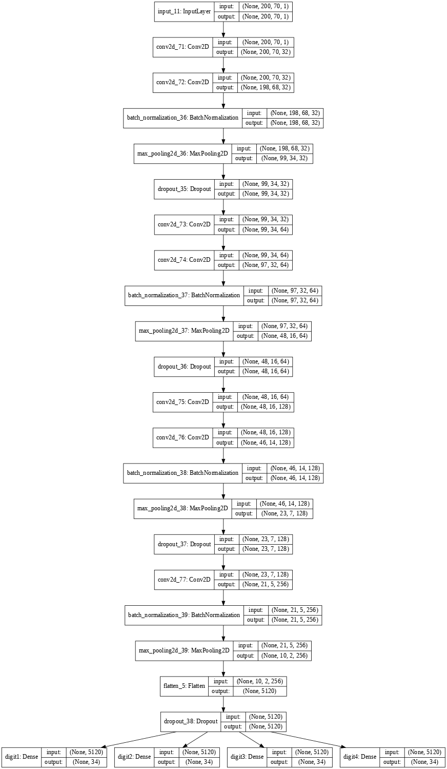
Figure 3.4: Our model for predicting the labels of the 4 letter CAPTCHA dataset.

1. 1.1 Examples of text CAPTCHAs increasing in difficulty both for Humans and Computers. Image collected from (starting from top) Wikipedia, JCAPTCHA, JCAPTCHA, Pixprofit, Wikipedia,  PayPal, and  Knpbundles post.
2. 1.2 Types of CAPTCHAS. (Picture Courtesey: IIHglobaland Wikipedia).
3. 1.3 Types of CAPTCHAS. (Picture Courtesey: IIHglobal, , and Dice CAPTCHA)
4. 1.4 Types of CAPTCHAS. (Picture Courtesey: Seosmarty, and Anime)
5. 2.1 Captcha 4 letter dataset available from Kaggle.
6. 2.2 The initial distribution of the letters for the Captcha (4 letter) dataset.
7. 2.3 Separable characters and their frequencies from Captcha 4 letter dataset.
8. 2.4 The extraction of separable characters using algorithm  1 for creation of c4l-16x16_550 dataset.
9. 2.5 Sample of c4l-16x16_550 dataset
10. 2.6 Frequency of characters obtained from c4l-16x16_550 dataset
11. 2.7 t-SNE cluster of c4l-16x16_550 dataset in 2D.
12. 2.8 t-SNE cluster of c4l-16x16_550 dataset in 2D with actual images.
13. 2.9 t-SNE cluster of c4l-16x16_550 dataset in 3D.
14. 2.10 JAM website containing simple CAPTCHA. (Source: https://joaps.iitk.ac.in/)
15. 2.11 A simple labeller to label the CAPTCHA.
16. 2.12 Removal of lines from the JAM CAPTCHA.
17. 2.13 t-SNE cluster of resized_JAM dataset in 2D with actual images.
18. 2.14 Distribution of resized_JAM CAPTCHA dataset.
19. 2.15 t-SNE cluster of resized_JAM dataset in 2D.
20. 2.16 Segmentation of JAM CAPTCHA.
21. 2.17 t-SNE cluster of resized_JAM dataset in 3D.
22. 2.18 The initial distribution of the letters for 50% of Multicolor CAPTCHA.
23. 2.19 The initial distribution of the letters for the CAPTCHA-version-2 dataset.
24. 2.20 Sample of CAPTCHA-version-2 dataset.
25. 2.21 Sample of 100000-labeled-captchas dataset.
26. 2.22 The initial distribution of the letters for the 100000-labeled-captchas.
27. 2.23 The initial distribution of the letters for the Faded CAPTCHA.
28. 2.24 Sample of the faded dataset.
29. 2.25 Sample of 100000-labeled generated Railway CAPTCHA dataset.
30. 2.26 Sample of the Circle CAPTCHA dataset.
31. 2.27 The initial distribution of the letters for the Circle CAPTCHA dataset.
32. 2.28 Sample of the sphinx CAPTCHA dataset.
33. 2.29 The initial distribution of the letters for the sphinx CAPTCHA dataset.
34. 2.30 Sample of the fish eye CAPTCHA dataset.
35. 2.31 The initial distribution of the letters for the fish eye CAPTCHA.
36. 2.32 Sample of the mini CAPTCHA dataset.
37. 2.33 The initial distribution of the letters for the mini CAPTCHA.
38. 2.34 Sample of multicolor CAPTCHA dataset.
39. 3.1 Performing adaptive thresholding of Binary Inverse before passing it to the model.
40. 3.2 Summary of the model for 3.4.
41. 3.3 The summary of 30 epochs for the model 3.4.
42. 3.4 Our model for predicting the labels of the 4 letter CAPTCHA dataset.
43. 3.5 The visualizations of the features in a fully trained model when passed a CAPTCHA of FR8U, for Figure 3.4.
44. 3.6 Plot for the training accuracy of our model.
45. 3.7 Plot for the training loss of our model.
46. 3.8 Prediction of the model on unseen data.
47. 3.9 Summary of the Version 2 of the Model
48. 3.10 The epochs for version 2 of the model.
49. 3.11 Version 2 of the model for identifying individual characters.
50. 3.12 Prediction of the new model (3.11) on unseen data.
51. 3.13 Loss of the new model (3.11).
52. 3.14 The 3x3 kernels (filter) learned by the model (3.11) for layer 1.
53. 3.15 The weights learned by the model (3.11) for layers 1 to 24.
54. 3.16 The 3x3 kernels (filter) learned by the model (7.5) for layer 1.
55. 3.17 The weights learned by the model (7.5) for layers 1 to 26.
56. 4.1 CIFAR 10 like model for identifying individual characters.
57. 4.2 epochs.
58. 4.3 Accuracy of the model as shown in Figure  4.1
59. 4.4 Accuracy of the model as shown in Figure  4.1
60. 4.5 The prediction of the model from the individual characters
61. 4.6 The confusion matrix of the individual characters
62. 4.7 The visualizations of the features in a fully trained model when passed an image for letter 2.
63. 4.8 The visualizations of the features in a fully trained model when passed an image for letter L.
64. 4.9 The visualizations of the features in a fully trained model when passed an image for letter K.
65. 4.10 The visualizations of the features in a fully trained model when passed an image for letter P.
66. 4.11 The wrong classification of the model.
67. 4.12 The Alex net type architecture. Created using https://alexlenail.me/NN-SVG/.
68. 4.13 The 3x3 kernels (filter) learned by the model (4.1) for layer 1.
69. 4.14 The weights learned by the model (4.1) for layers 1 to 16.
70. 5.1 Varying the value of $k$ to get the best testing accuracy.
71. 5.2 The confusion matrix of the resized_JAM dataset.
72. 6.1 Accuracy obtained from the AlexNet type model (8.1).
73. 6.2 Loss obtained from the AlexNet type model (8.1).
74. 6.3 The weights learned by the model (8.1) for layers 1 to 16.
75. 6.4 Summary of the AlexNet type model for classifying the labels of CAPTCHA-version-2 dataset.
76. 6.5 Summary of epochs for the model (6.4).
77. 6.6 The weights learned by the model (6.12) for layers 1 to 16.
78. 6.7 Summary of the model for classifying the labels of CAPTCHA-version-2 dataset.
79. 6.8 Model for training CAPTCHA-version-2 dataset.
80. 6.9 Summary of epochs for the model (6.8).
81. 6.10 Accuracy of the model (6.8).
82. 6.11 Loss of the model (6.8).
83. 6.12 Tensorboard Visualization of the structure of the model (6.8).
84. 6.13 The visualizations of the features in a fully trained model for Model 6.12 when passed a CAPTCHA containing the text 5mfff.
85. 6.14 The visualizations of the features in a fully trained model for Model 6.12 when passed a CAPTCHA containing the text 7cdge.
86. 6.15 The visualizations of the features in a fully trained model for Model 6.12 when passed a CAPTCHA containing the text cpc8c.
87. 6.16 The 3x3 kernels (filter) learned by the model (6.12) for layer 1.
88. 7.1 Summary of the epochs after training the model (7.5).
89. 7.2 Predictions with the model (7.5).
90. 7.3 The weights learned by the model (7.5) for layers 1 to 26.
91. 7.4 Model (7.5) for identifying 1L-labelled-CAPTCHA dataset.
92. 7.5 CIFAR 10 like model for identifying individual characters.
93. 7.6 Training Accuracy for the model (7.5).
94. 7.7 Training Loss for the model (7.5).
95. 7.8 The 3x3 kernels (filter) learned by the model (7.5) for layer 1.
96. 7.9 The visualizations of the features in a fully trained model (7.5) when passed a CAPTCHA containing the text r543n.
97. 8.1 Alex-Net type model for multi-label classification.
98. 8.2 epochs for faded CAPTCHA.
99. 8.3 The accuracy and Loss obtained from the model when visualized via tensorboard.
100. 8.4 The prediction of the model with 100% accuracy on unseen data.
101. 9.1 Summary of the model for 13.3.
102. 9.2 epochs for circle CAPTCHA.
103. 9.3 Keras model structure for Circle CAPTCHA.
104. 9.4 Accuracy of the model (9.3).
105. 9.5 Loss of the model (9.3).
106. 9.6 Predictions of the model (9.3).
107. 10.1 Summary of the model for 13.3.
108. 10.2 epochs for sphinx CAPTCHA.
109. 10.3 Tensorboard Visualization of the structure of the model (6.8).
110. 10.4 Accuracy of the model (10.3).
111. 10.5 Loss of the model (10.3).
112. 10.6 Predictions of the model (10.3).
113. 11.1 Summary of the AlexNet type model for classifying the labels of fish eye CAPTCHA dataset.
114. 11.2 Summary of epochs for the model (6.8).
115. 11.3 Tensorboard Visualization of the structure of the model (6.8).
116. 11.4 Accuracy of the model (11.3).
117. 11.5 Loss of the model (11.3).
118. 11.6 Predictions of the model (11.3).
119. 12.1 Summary of the model for 13.3.
120. 12.2 epochs for mini CAPTCHA.
121. 12.3 Keras model structure for Circle CAPTCHA.
122. 12.4 Accuracy of the model (12.3).
123. 12.5 Loss of the model (12.3).
124. 12.6 Predictions of the model (12.3).
125. 13.1 Summary of the model for 13.3.
126. 13.2 The summary of 9 epochs for the model 13.3.
127. 13.3 Our model for predicting the labels of the multicolor CAPTCHA dataset.
128. 13.4 Plot for the training accuracy of our model.
129. 13.5 Plot for the training loss of our model.
130. 13.6 Prediction of the new model (13.3) on unseen data.
131. 14.1 Summary of the vanilla model (14.3) for railway 3 letter CAPTCHA dataset.
132. 14.2 Summary of the epochs for the vanilla model (14.3) for railway 3 letter CAPTCHA dataset.
133. 14.3 The vanilla model for railway 3 letter CAPTCHA dataset.
134. 14.4 Training Accuracy for the vanilla model (14.3).
135. 14.5 Training Loss for the vanilla model (14.3).
136. 14.6 The preprocessing done to improve accuracy before feeding it to the model (14.3).
137. 14.7 A CAPTCHA of 254 was given to the layer of the model (14.3) for visualizations.
138. 14.8 Predictions of the model (14.3).
139. 14.9 The visualizations of the features in a fully trained model 14.3 when passed a CAPTCHA containing the characters 254.
140. 14.10 Model 14.12 Summary for cracking 4-letter railway CAPTCHA.
141. 14.11 Model 14.12 Summary.
142. 14.12 Our vanilla model for cracking 4-letter railway CAPTCHA.
143. 14.13 Training Accuracy for the model (14.12).
144. 14.14 Training Loss for the model (14.12).
145. 14.15 Predictions of the model (14.12).
146. 14.16 Model (14.19) Summary.
147. 14.17 Summary for model’s (14.19) epochs
148. 14.18 Summary for model’s (14.25) epochs
149. 14.19 Our vanilla model for cracking 5-letter railway CAPTCHA.
150. 14.20 Training Accuracy for our vanilla model (14.19).
151. 14.21 Predictions of the vanilla model (14.25).
152. 14.22 Training Loss for the vanilla model (14.19).
153. 14.23 Predictions of the vanilla model (14.19).
154. 14.24 Model (14.25) Summary.
155. 14.25 Our vanilla model for cracking 6-letter railway CAPTCHA.
156. 14.26 Training Accuracy for vanilla model (14.25).
157. 14.27 Training Loss for vanilla model (14.25).
158. 14.28 Model’s graph as visualized in tensorboard (14.25).
159. 14.29 Model (14.32) Summary.
160. 14.30 Summary for model’s (14.32) epochs
161. 14.31 A subset of samples given to the model (14.10)
162. 14.32 Our vanilla model for cracking 7-letter railway CAPTCHA.
163. 14.33 Training Accuracy for vanilla model (14.32).
164. 14.34 Training Loss for vanilla model (14.32).
165. 14.35 Predictions of the model (14.32).
166. 14.36 Distribution of the data for the various labels of the Railway CAPTCHA dataset for (3,4 and 5 letter images).
167. 14.37 Distribution of the data for the various labels of the Railway CAPTCHA dataset (for 6 and 7 letter images).
168. 14.38 The complexity of the model increases with the length of the CAPTCHA, data from table (14.1).

List of Tables

1. 14.1 Table showing that the length of the CAPTCHA is directly proportional to the complexity.

Chapter 1 Introduction

In a reverse turing test  [1] the roles between computers and humans has been reversed. Alan Turing  [2, 3] in 1950, developed the Turing test to tell computers and humans apart via imitation game . The rule of the imitation game is simple, it is played with three people, a man (A), a woman (B) and an interrogator (C). The interrogator stays in a room apart from the other two and the objective of the interrogator is to determine which of the two is man and which is a woman. He may consider them as labels X and Y. The interrogator is allowed to put questions to both of A and B and will get answer in text, which will not introduce any bias towards determining the objective of the interrogator. Turing predicted about 70 years ago that it will be possible to program computers with storage capacity of about 10⁹ states to make them play this imitation game so well that an average interrogator will not have more than 70 percent chance of making the right identification after five minutes of questioning, and here we are in 2020 where we cannot distinguish between a bot and a person in online forums and gaming sites!

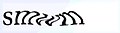
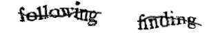
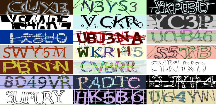
Figure 1.1: Examples of text CAPTCHAs increasing in difficulty both for Humans and Computers. Image collected from (starting from top) Wikipedia, JCAPTCHA, JCAPTCHA, Pixprofit, Wikipedia,  PayPal, and  Knpbundles post.

Reverse Turing test deals with computer (here server) acting as an interrogator and determining whether the user is a bot (computer) or a human. Here the computer is said to pass the Turing test if it always correctly recognizes a human as human and a computer as itself. In today’s world there is a necessity to prevent bots from spamming, creating multiple account and jamming the resource of a particular website. There are various ways through which the reverse Turing Test is implemented by websites and service providers to stop illegitimate access of their contents by hackers and spammers.

1.1 CAPTCHA

One method for performing reverse Turing test is through CAPTCHA which is an acronym for Completely Automated Public Turing test to tell Computers and Humans Apart. They are designed to protect online sites from bot attacks which may create automated fake profiles to scam people. CAPTCHAs are designed in such a way that they can be solved by humans easily but not by a computer. This user identification procedure has received criticism from people with disabilities and also those people who thinks their everyday work is being slowed down by solving a typical CAPTCHA for 10 seconds.

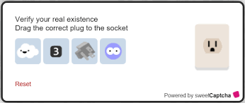
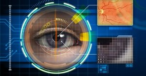
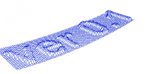
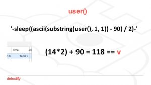
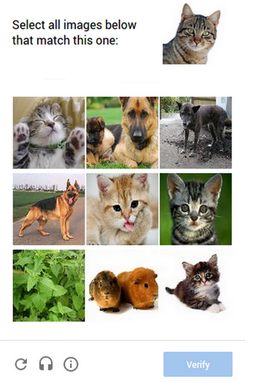
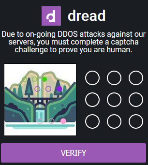
Figure 1.2: Types of CAPTCHAS. (Picture Courtesey: IIHglobaland Wikipedia).

There are different types of CAPTCHAs, a subset of text CAPTCHAs is shown in Figure  1.1. We see that the text CAPTCHAs are getting difficult to solve by humans, while the Hackers comes up with more powerful CAPTCHA breaker every day. Automated scripts  [4] should not be more successful than 1 in 10,000 (0.01%) for any type of attack, while the human’s success rate should approach 90%. This ensures that humans have to endure less pain in solving CAPTCHAs.

1.2 Types of CAPTCHAs

There are different types of CAPTCHAs as shown in Figure  1.2 and Figure  1.3. Sweet CAPTCHA makes you match easy images instead of reading twisted texts. Playthru CAPTCHA replaces the pain of reading texts via fun microgames, where humans get through easily while automated bots are kept out. Biometric test is the next generation CAPTCHA, that comes with facial and speech recognition based on knowledge set. Text message verification helps the site to verify the actual mobile number of users instead of traditional User IDs and Passwords. Image based CAPTCHA include confident CAPTCHA and Picture identification CAPTCHA which the user needs to recognize and select a set of images which is easy for humans but difficult for bots. Google’s reCAPTCHA helps sites to be protected from spambots. There is another type of CAPTCHA which lets users to solve word problems and math problems. Time based CAPTCHA analyses the time required by the user to fill forms and from the analysis it can predict whether the user is a bot or human. There is 3D CAPTCHA which are difficult for bots to decipher but easy for humans. Add based CAPTCHA provides some extra revenue to the site by providing add based text to decipher. There is drag and drop CAPTCHA which is an intuitive way of verifying different humanity tasks which are difficult for robots. Tic-Tac-Toe CAPTCHAs helps to entertain the user by playing mini games.

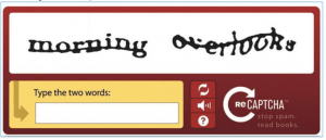
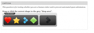
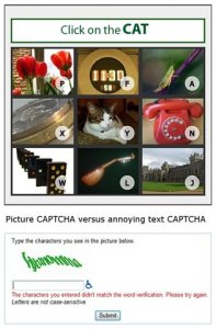
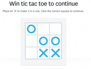
Figure 1.3: Types of CAPTCHAS. (Picture Courtesey: IIHglobal, , and Dice CAPTCHA)

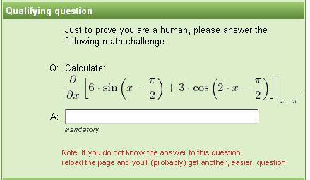
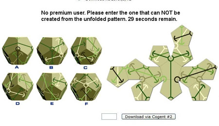
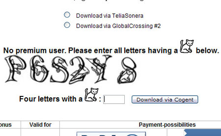
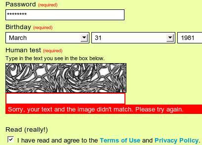
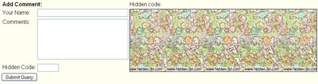
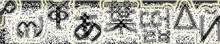
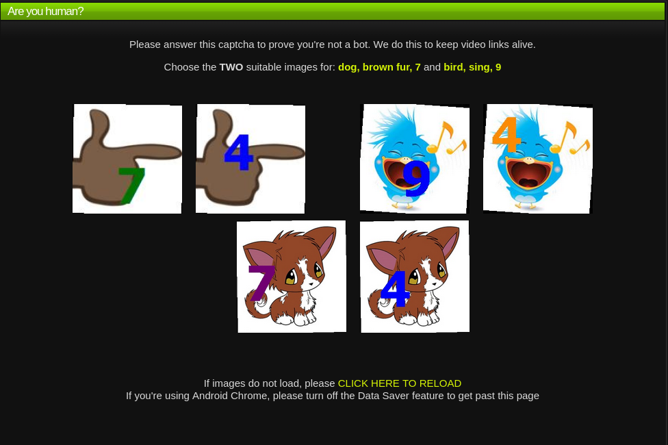
Figure 1.4: Types of CAPTCHAS. (Picture Courtesey: Seosmarty, and Anime)

CAPTCHAs can even be a little harder to do when there is a time limit to solve CAPTCHA and it may be even difficult for humans. The examples of such type of CAPTCHAs are shown in Figure  1.4. The first picture has some sort of partial differential equation solver, which is completely unnecessary, and is not designed for naive users. The second figure contains some really sophisticated paper folding problem which also needs some amount of time to solve. CAPTCHAs may be clumsy and undecipherable as shown in the corresponding figures. The second last figure’s CAPTCHA is formed from different languages, and would probably be suitable for Cipher Cracking Competitions. The last CAPTCHA is not so difficult for humans, but instead it needs to be solved very quickly and needs a lot of retry to get to the actual website.

1.3 Our Work

From the above discussions we find that there are various types of CAPTCHAs present to stop the nuisance of bots. We have seen that the ways to develop CAPTCHAs are increasing in complexity day by day. This leaves us to one question, is it worth it? We have worked in breaking of a certain subset of CAPTCHAs i.e., text-based image CAPTCHAs. The text-based CAPTCHAs are the backbone of Optical Character Recognition (OCR) task. These CAPTCHAs are modified day to day in such a way that it becomes hard for humans to understand and much more difficult for computers to decipher. We have tried some of the difficult CAPTCHAs and benchmarked those results, starting from the naive CAPTCHAs. We have also suggested what kind of technologies needs to be introduced to prevent the unauthorized access by bots.

Chapter 2 About the data

We have used some of the available open Kaggle data. Now we will discuss about the dataset used in this investigation.

2.1 Captcha (4 letter)

This dataset can be found online on Kaggle (https://www.kaggle.com/genesis16/captcha-4-letter) and the cleaned version can be found here (https://jimut123.github.io/blogs/CAPTCHA/data/captcha_4_letter.tar.gz). This dataset contains about 9955 PNG images of 4 letter CAPTCHA, some of which are closely connected as shown in Figure 2.1. The total size of the data is 10.4 M.B. The images have 3 channels, i.e., they have a Red Green and Blue component, and are of dimension 72x24. We have extracted the separable characters to form a simple dataset containing 32 characters. There were many such characters which were not separable and we have discarded such characters. From Figure 2.3 we can see that digits 0,1,I and O are missing from this CAPTCHA data. The original distribution of the characters of the dataset is shown in Figure 2.2.

Figure 2.1: Captcha 4 letter dataset available from Kaggle.

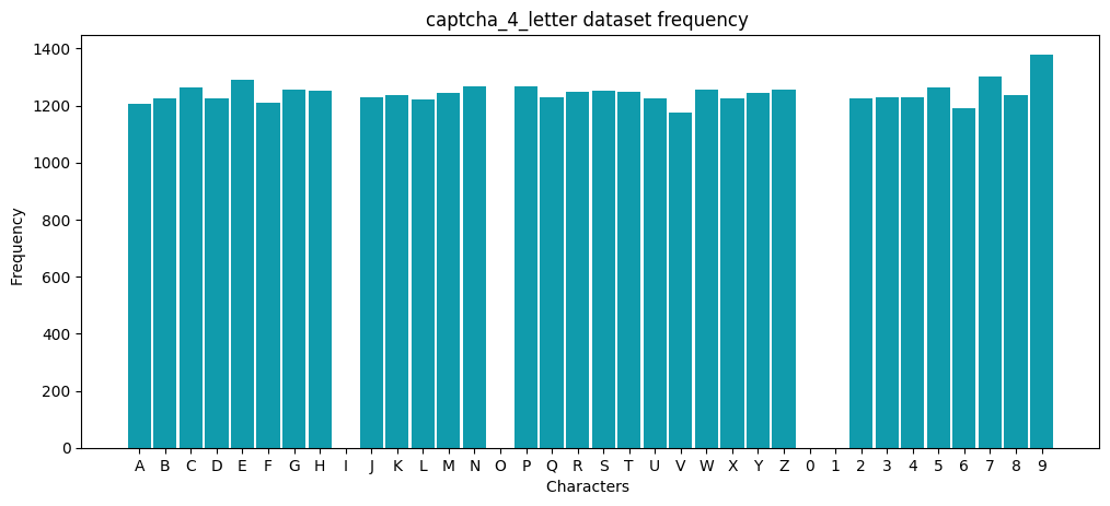
Figure 2.2: The initial distribution of the letters for the Captcha (4 letter) dataset.

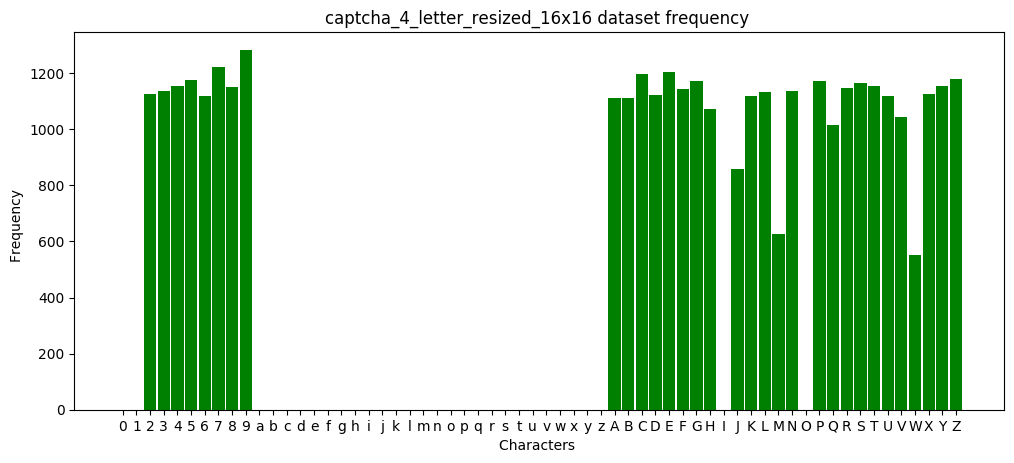
Figure 2.3: Separable characters and their frequencies from Captcha 4 letter dataset.

We have performed various algorithm on this data and created a modified dataset named c4l-16x16_550 using algorithm 1.

Input: $list\_of\_files\leftarrow All~{}the~{}files~{}needed~{}to~{}be~{}extracted$

Result: Extracted files

for each_file in list_of_files do

       $img\_file$ $\leftarrow$ read current file;

       $gray$ $\leftarrow$ convert image file to gray;

       $thresh$ $\leftarrow$ perform Otsu’s thresholding;  [5]

       $k$ = 0;

       $ROI\_number$ = 0;

       for $y\leftarrow 0$ to $img\_file.height()$ do

             $dummy$ = 0 ;

              // keeps track of separation

             for $x\leftarrow 0$ to $img\_file.width()$ do

                   if $thresh[x][y]==0$ then

                         $dummy$ = 1 ;

                          // separation found hence extract character

                         Level 2 extracted Ref Figure. 2.4.;

                        

                   end if

                  

             end for

            if $dummy$ == 1 && $k$ == 1  then

                   $start\_col$ $\leftarrow$ $y$;

                   $k$ $\leftarrow$ $k$ + 1;

                  

             end if

            if $dummy$ == 0 && $k$ $>$ 2  then

                   $end\_col$ $\leftarrow$ y;

                   $k1$ $\leftarrow$ 0;

                   $extract\_img$ $\leftarrow$ $thresh[:,start\_col-2:end\_col+1].copy()$

             end if

            

            for $x1\leftarrow 0$ to $extract\_img.width()$ do

                   $dummy1$ = 0 ;

                    // keeps track of separation

                   for $y1\leftarrow 0$ to $extract\_img.height()$ do

                         if $extract\_img[x1][y1]==0$ then

                               $dummy1$ = 1 ;

                                // separation found hence extract character

                              

                         end if

                        

                   end for

                  if $dummy1$ == 1 && $k1$ == 1  then

                         $start\_row$ $\leftarrow$ $x1$;

                         $k1$ $\leftarrow$ $k1$ + 1;

                        

                   end if

                  if $dummy1$ == 0 && $k1$ $>$ 2  then

                         $end\_row$ $\leftarrow$ $x1$;

                         Level 3 extracted Ref Figure. 2.4.;

                         $ROI$ = $extract\_img[start\_row-2:end\_row+1,:].copy()$;

                         Save the extracted region of interst

                   end if

                  

             end for

            

       end for

      

end for

Algorithm 1 Region of Interest Extractor

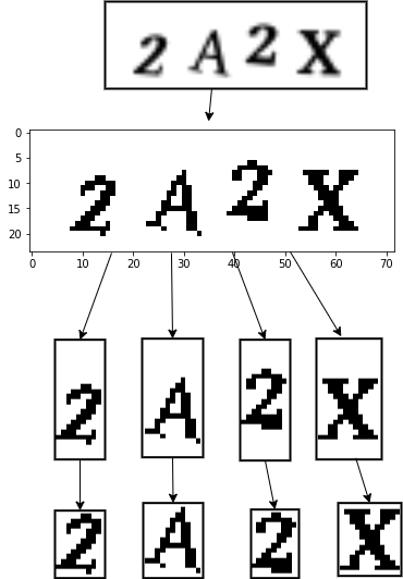
Figure 2.4: The extraction of separable characters using algorithm  1 for creation of c4l-16x16_550 dataset.

2.2 Creation of c4l-16x16_550 dataset

This is the modified version of the data created by extracting each image and performing Otsu’s  [5] thresholding on the extracted image as shown in Figure  2.5. The dataset can be obtained from here (https://jimut123.github.io/blogs/CAPTCHA/data/c4l-16x16_550.tar.gz). Otsu’s thresholding is an unsupervised and nonparametric method for automatic threshold selection which utilizes the zeroth and first order cumulative moments  [5] of gray level histogram.

Figure 2.5: Sample of c4l-16x16_550 dataset

Now the dataset contains 32 characters of dimension 16x16 as shown in Figure 2.6. This dataset can be used for performing benchmarks just like MNIST dataset. The real challenge here is that there are 550 images for each character, and one need to get a good model with such less data.

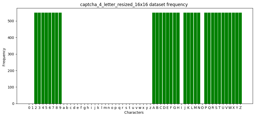
Figure 2.6: Frequency of characters obtained from c4l-16x16_550 dataset

2.3 t-SNE cluster for c4l-16x16_550 dataset

t-Distributed Stochastic Neighbor Embedding (t-SNE) visualizes high

Figure 2.7: t-SNE cluster of c4l-16x16_550 dataset in 2D.

dimensional data by giving each datapoint a location in three or two-dimensional map. This technique is much easier to optimize, and gives better visualizations by reducing the tendency to crowd points together in the center of the map. Stochastic Neighbor Embedding (SNE) converts the high dimensional Euclidean distance between datapoints into conditional probabilities  [6] that represent similarities. The similarity between two datapoints $x_{j}$ and $x_{i}$ is the conditional probability $p_{j|i}$, that $x_{i}$ would pick neighbor as $x_{j}$ if neighbors were picked in proportion to their probability density under a Gaussian centered at $x_{i}$. So, from the nature of the Gaussian distribution we can say that for nearby points $p_{j|i}$ is relatively high, whereas for widely spread datapoints $p_{j|i}$ will be infinitely small.

$$p_{j|i}=\frac{\exp(-||x_{i}-x_{j}||\textsuperscript{2}/2\sigma_{i}\textsuperscript{2})}{\sum_{k\neq i}\exp(-||x_{i}-x_{k}||\textsuperscript{2}/2\sigma_{i}\textsuperscript{2})}$$ (2.1)

Here $\sigma_{i}$ is the variance of the Gaussian that is centered on datapoint $x_{i}$. We can do the same for $y_{i}$ and $y_{j}$, the low dimensional counterparts  [6] of the high dimensional datapoints $x_{i}$ and $x_{j}$, which we denote by $q_{j|i}$.

$$q_{j|i}=\frac{\exp(-||y_{i}-y_{j}||\textsuperscript{2})}{\sum_{k\neq i}\exp(-||y_{i}-y_{k}||\textsuperscript{2})}$$ (2.2)

If the map points $y_{i}$ and $y_{j}$ correctly model the similarity between the high dimensional data points, i.e., $x_{i}$ and $x_{j}$ then both the conditional probabilities $p_{j|i}$ and $q_{j|i}$ will be equal. This modelling is done through Kullback-Leiber divergence  [6] and SNE minimizes the sum of these overall datapoints using gradient descent method.

The cost function C is given by

$$C=\sum_{i}KL(P_{i}||Q_{i})=\sum_{i}\sum_{j}p_{j|i}\log\frac{p_{j|i}}{q_{j|i}}$$ (2.3)

Here, $P_{i}$ represents the conditional probability distribution over all other data points given data points $x_{i}$, and $Q_{i}$ represents the conditional probability distribution over all map points given map point $y_{i}$.

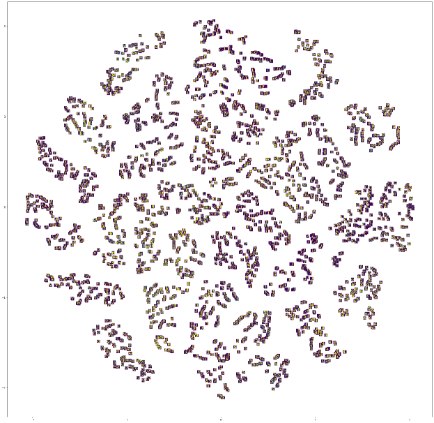
Figure 2.8: t-SNE cluster of c4l-16x16_550 dataset in 2D with actual images.

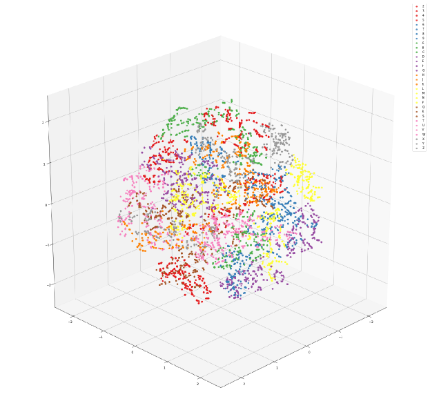
Figure 2.9: t-SNE cluster of c4l-16x16_550 dataset in 3D.

t-SNE uses symmetrized version of the SNE cost function with gradient descent which are easier to optimize and a Student-t distribution  [6] rather than a Gaussian. Figure 2.7 shows the visualisation of the data in 2-dimensional space, similarly Figure 2.8 shows the same visualization but with the actual character that forms the part of the visualization. Figure  2.9 shows the 3-dimensional visualization of the same datapoints.

2.4 JAM CAPTCHA dataset

We found this CAPTCHA on IIT-JAM’s website as shown in Figure 2.10. This is an interesting problem to solve since the CAPTCHA has a strike-though in it, to create confusion for machines to classify this CAPTCHA. We thought to ourselves whether this is really a good CAPTCHA? We created a dataset by scraping almost 10,000 of CAPTCHAs and labelling only 308 of them using a tool we created as shown in Figure 2.11. This tool can be used to label any kind of CAPTCHA without manually selecting rename every time. The initial size of the CAPTCHA was 100x40x3 with the three channels (R,G,B). We needed to modify this data to convert to grayscale since this CAPTCHA doesn’t really makes sense to contain 3 channels. The only color that it had was white in black background. We also applied a certain thresholding so that the image turns to pure binary file with just one channel.

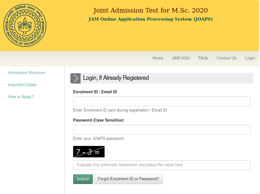
Figure 2.10: JAM website containing simple CAPTCHA. (Source: https://joaps.iitk.ac.in/)

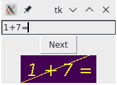
Figure 2.11: A simple labeller to label the CAPTCHA.

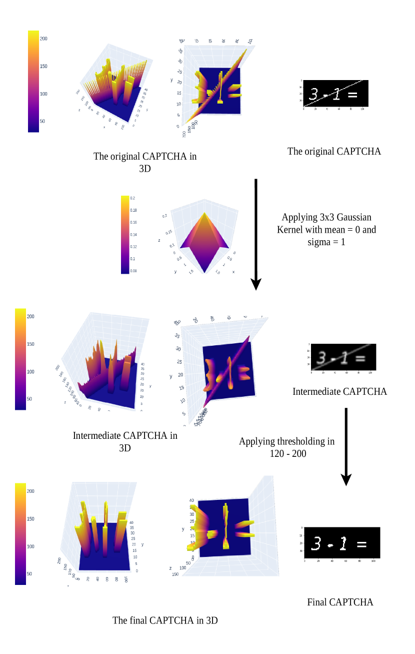
Figure 2.12: Removal of lines from the JAM CAPTCHA.

Since we want to try out a simple model on this CAPTCHA, we needed to remove the strike-through in it. We found that this CAPTCHA has very similar kind of font style with no change in them. We thought that it can be easily solved with the help of $k$-Nearest Neighbor (KNN) algorithm, if we can somehow remove the noise and partition the characters with the segmentation algorithm 1. The removal of the line was easy. The procedure for removal of lines for each image is shown in Figure 2.12. First, we take the converted thresholded CAPTCHA and pass it through a gaussian filter [7] with $\sigma$ = 1 and $\mu$ = 0. We do this because the strike is thinner than the bold numbers. This will make the strike lower in intensity when seen in 3D. After this we will apply a threshold, i.e., every value of intensity that is less than 120 will turn to 0 and the values above 200 will turn to 255 and hence that will be the final resultant thresholded CAPTCHA as shown in Figure 2.12 below.

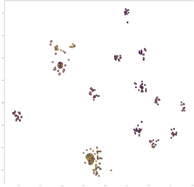
Figure 2.13: t-SNE cluster of resized_JAM dataset in 2D with actual images.

2.5 Classifying digits through k-NN with the resized_JAM dataset

For training in $k$-NN we created the resized_JAM dataset. This was achieved by applying algorithm 1 in the final image. The process of segmentation is shown in Figure 2.16. The segmentation resulted in uneven sized images of each of the characters present in the image. Then we resized each of them in 20x20 images for creating the resized_JAM dataset. The dataset can be found here (https://jimut123.github.io/blogs/CAPTCHA/data/resized_JAM.tar.gz). The distribution of characters of the dataset is shown in Figure 2.14.

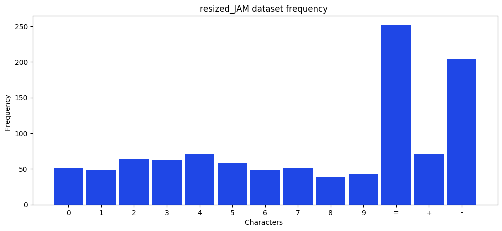
Figure 2.14: Distribution of resized_JAM CAPTCHA dataset.

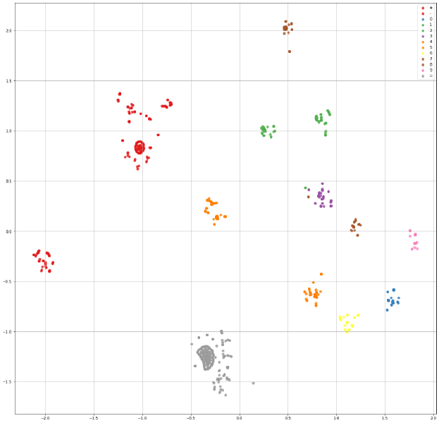
Figure 2.15: t-SNE cluster of resized_JAM dataset in 2D.

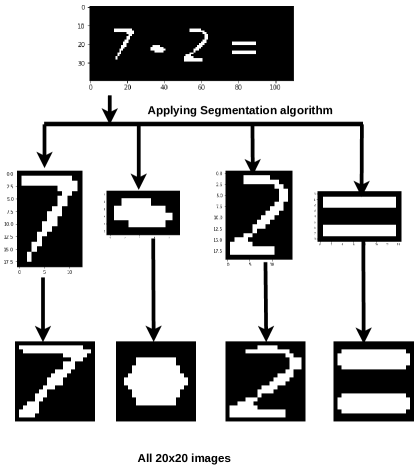
Figure 2.16: Segmentation of JAM CAPTCHA.

We see that there is a relatively uneven distribution in the case of this dataset. This will not create any major problem. Since the data is relatively low, so we can use the $k$-NN classifier. The t-SNE plot of the data in 2D is shown in Figure 2.15. The same plot with the actual images is shown in Figure 2.13. The 3D plot is shown in Figure 2.17.

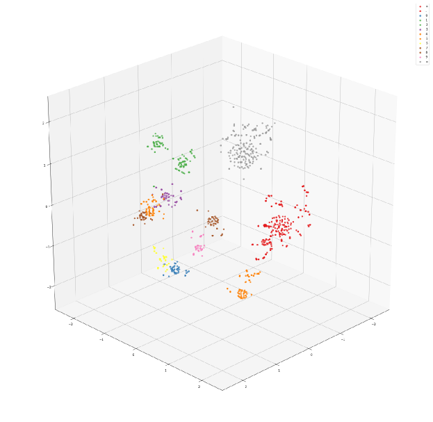
Figure 2.17: t-SNE cluster of resized_JAM dataset in 3D.

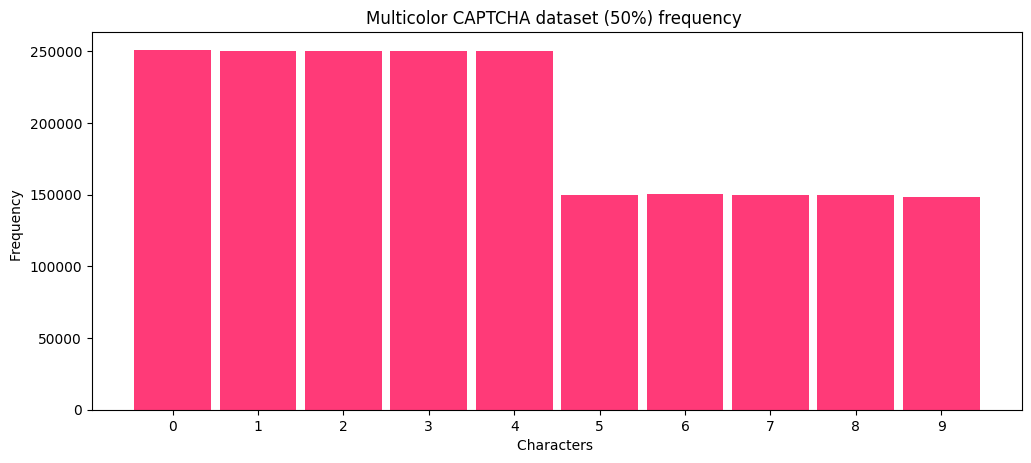
Figure 2.18: The initial distribution of the letters for 50% of Multicolor CAPTCHA.

2.6 CAPTCHA-version-2

This dataset can also be found online on Kaggle (https://www.kaggle.com/fournierp/captcha-version-2-images). The cleaned version can be found here (https://jimut123.github.io/blogs/CAPTCHA/data/captcha_v2.tar.gz). There are two sets of folders each containing 1070 images, the total size of the dataset is about 21.5 MB. The images have 3 channels, i.e., they have a Red Green and Blue component, and are of dimension 200x50. The dataset comprises of small letter character ASCII characters (i.e., a-z) and digits (0-9). It is 5 letter CAPTCHA and the images are cluttered to create confusion as shown in Figure 2.20. The initial distribution of the characters of the dataset is shown in Figure 2.19, which is almost uniform except the letter n.

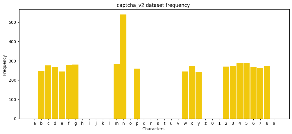
Figure 2.19: The initial distribution of the letters for the CAPTCHA-version-2 dataset.

Figure 2.20: Sample of CAPTCHA-version-2 dataset.

Figure 2.21: Sample of 100000-labeled-captchas dataset.

2.7 100000-labeled-captchas

This dataset can also be found online on Kaggle https://www.kaggle.com/digdeepbro/100000-labeled-captchas. The cleaned version can be found here on figshare (https://dx.doi.org/10.6084/m9.figshare.12046881.v1). The dataset is about 215 MB on figshare. The original dataset found on Kaggle contained only the alpha values, our processed version contains binary images by applying Otsu’s thresholding as shown in Figure 2.21 (right). It is necessary to convert the dataset to binary value for getting better predictions and we also need to inverse the colours, since white is represented by intensity value of 255 on grayscale and black by 0. For training it is necessary to take the most prominent pattern to be higher value and less important patterns to be smaller for the network to learn faster. It is also uploaded to figshare because we are taking the advantage of Google’s free resource called Collaboratory here, which provides free GPU and 25GB of RAM on cloud, since Kaggle doesn’t allow to directly download files to remote server by performing wget, we needed to reupload the cleaned version on figshare. This ensures that we can reuse the code without further modification and share the colab notebook with anybody. We could also upload the contents in drive, but from my earlier experience, I have found that the GPU doesn’t work on such data after sometime since the server has to relocate the old data every time, on the other hand by this method, it is downloading from figshare with about 25MB/s speed and storing it on temporary storage so that we can perform fast computations easily. The initial distribution of the characters of the dataset is shown in Figure 2.22, which is almost uniform.

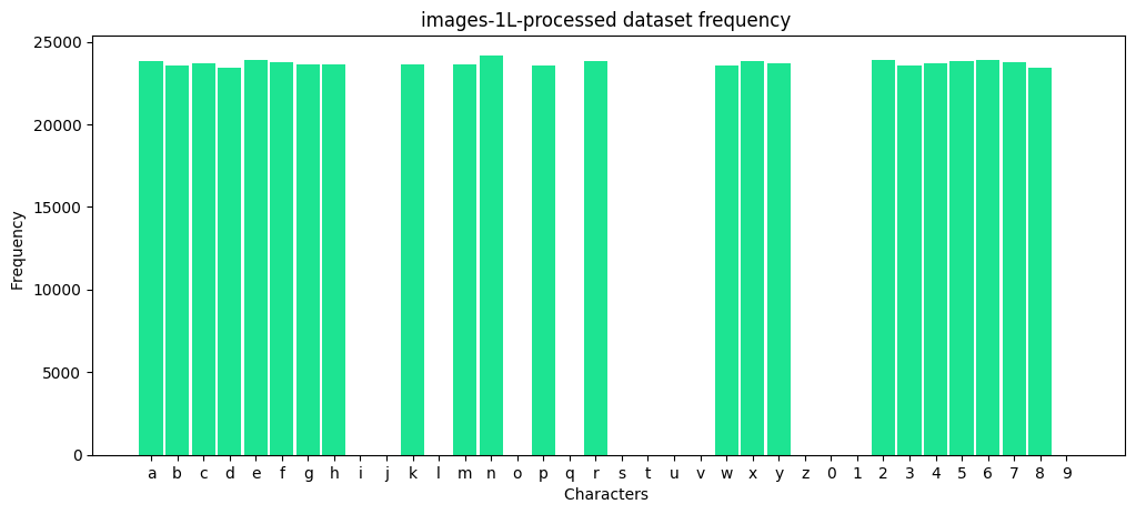
Figure 2.22: The initial distribution of the letters for the 100000-labeled-captchas.

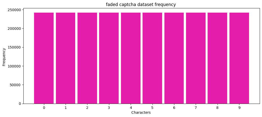
Figure 2.23: The initial distribution of the letters for the Faded CAPTCHA.

2.8 Faded CAPTCHA

We have found an open sourced CAPTCHA data generator and created a dataset called Faded CAPTCHA dataset. The original source code for the generator can be found here https://github.com/JackonYang/captcha-tensorflow. The faded CAPTCHA dataset comprises of about 604800 files of dimension 100x120x3 for the three channels. The charcters present in this CAPTCHA data is from 0-9. A sample of the data is shown in Figure 2.24. The distribution of the characters of faded CAPTCHA dataset is shown in Figure 2.23. This shows that the CAPTCHA has a uniform distribution of characters which will help it generalise on the test dataset better. The dataset comprises of about 10 folders and the link to each of them is given in the Appendix section. The total size of the dataset is about 3.7 GiB.

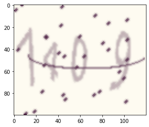
Figure 2.24: Sample of the faded dataset.

2.9 Railway CAPTCHA

This dataset is a created synthetically by getting hold of the source code from GitHub. The original repository can be found here https://github.com/JasonLiTW/simple-railway-captcha-solver. We have modified this CAPTCHA generator a bit and created our own dataset comprising of 100K images each for 3,4,5,6, and 7 letter CAPTCHAs as shown in Figure 2.25. The dataset for 3,4,5,6, and 7 letter CAPTCHAs can be found from https://dx.doi.org/10.6084/m9.figshare.12045249.v1, https://dx.doi.org/10.6084/m9.figshare.12045288.v1, https://dx.doi.org/10.6084/m9.figshare.12045294.v1, https://dx.doi.org/10.6084/m9.figshare.12045657.v1 and https://dx.doi.org/10.6084/m9.figshare.12053937.v1 respectively.

   

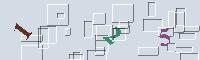
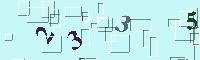
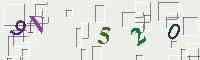
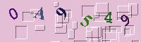
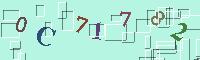
Figure 2.25: Sample of 100000-labeled generated Railway CAPTCHA dataset.

The authors of the original data generator claims that this CAPTCHA can be found to be active on Taiwan railway booking website. The CAPTCHA is generated by applying random transformation to images formed by Courier New-Bold and Times New Roman-Bold fonts.

2.10 Circle CAPTCHA

We found this type of CAPTCHA from https://github.com/py-radicz/captcha_gen. We modified a bit, and created our own dataset. The dataset can be found from here https://figshare.com/articles/captcha_gen/12286766. A sample of the circular CAPTCHA is shown in Figure 2.26. The distribution of the letters of the Circle CAPTCHA can be shown in Figure 2.27. This shows that the circle CAPTCHA consists of all the smaller case (a-z) letters and numbers (0-9) as label in its contents. The dataset comprises of 437.58 MB data, which is of dimension 35x120x3 (for the three channels). The dataset comprises of about 222K samples.

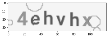
Figure 2.26: Sample of the Circle CAPTCHA dataset.

Figure 2.27: The initial distribution of the letters for the Circle CAPTCHA dataset.

2.11 The Sphinx CAPTCHA

We found the open source code for this type of CAPTCHA from https://github.com/davidpalves/sphinx-captcha. One sample of the Sphinx CAPTCHA is shown in Figure 2.28. The sphinx CAPTCHA is a relatively difficult CAPTCHA because it has a line (strikethrough through it), with relatively same thickness of the letters and noise of different color all over it. The distribution of the letters from the sphinx captcha dataset can be found in Figure 2.29. The images of the sphinx CAPTCHA dataset have a dimension of about 368x123x3 for the three channels. There are about 990K images which is close to 1M. The link to the figshare version of the dataset can be found in the appendix section. The dataset comprises of 34 parts of tar.gz all uploaded in figshare. The whole size of the dataset is about 12.2 GiB. This dataset contains only some of the characters from A-Z range, with some missing characters.

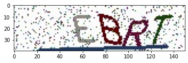
Figure 2.28: Sample of the sphinx CAPTCHA dataset.

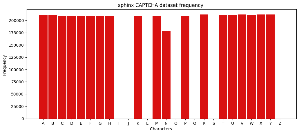
Figure 2.29: The initial distribution of the letters for the sphinx CAPTCHA dataset.

2.12 Fish Eye CAPTCHA

We found the Java source code from GitHub, for this type of CAPTCHA and created our own flexible fish eye CAPTCHA generator. One sample of the fish eye type CAPTCHA is shown in Figure 2.30. We can see there is a lot of variety in this type of CAPTCHA. This type of CAPTCHA poses a real challenge to machine learning systems. There is grid, a line and bold letters which is occluded by lines of different colors. The deep learning model needs to learn each of the representation of the CAPTCHA dataset. There is a total of 2 million sample in the generated dataset. The dataset can be found from this url (https://figshare.com/articles/Fish_Eye/12235946). Each sample of the data has a dimension of about 50x200x3 for the three channels. The data distribution of the characters for this dataset can be shown in Figure 2.31.

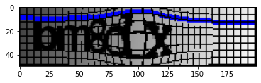
Figure 2.30: Sample of the fish eye CAPTCHA dataset.

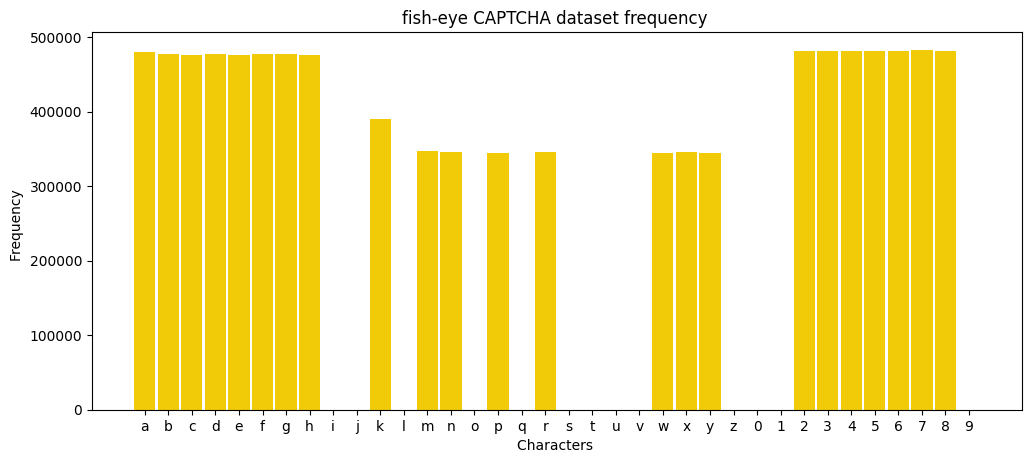
Figure 2.31: The initial distribution of the letters for the fish eye CAPTCHA.

2.13 Mini CAPTCHA

We found the open source code from https://github.com/imanhpr/miniCaptcha, and modified a bit to generate the actual CAPTCHA generator. The dataset has about 1 million samples of size 368x159x3 (for three channels). A sample from the dataset is shown in Figure 2.32. The distribution of the letters of the dataset is shown in Figure 2.33. There are a variety of colours that is present in the CAPTCHA dataset. The dataset can be found from here https://figshare.com/articles/Mini_Captcha/12286697. The distribution shows that there are all the letters present in the English alphabet, both upper case [A-Z] and lower case [a-z] along with digits [0-9], which makes it challenging task for computers to classify about 62 classes all at once.

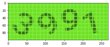
Figure 2.32: Sample of the mini CAPTCHA dataset.

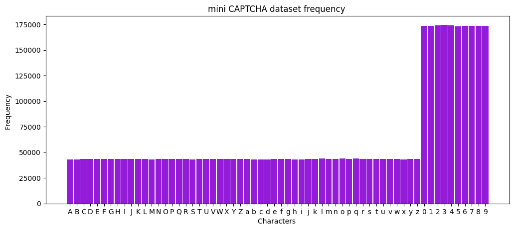
Figure 2.33: The initial distribution of the letters for the mini CAPTCHA.

2.14 Multicolor CAPTCHA

We found the original source code for this type of CAPTCHA on this link https://github.com/J-Rios/multicolor_captcha_generator. We have generated about 1 Million CAPTCHA data, but used only 50% of the original dataset. The link for the dataset can be found from the appendix section. We have used a difficulty level of 4 for the generation of the data. The highest difficulty is level 5, which has got more different types of colors, but is similar to this type of data. The actual problem is that these CAPTCHAs are slow to generate. A sample of the CAPTCHAs generated are shown in Figure 2.34. There is extra back background that is present in the original version of the dataset, which needs to be cropped as shown in the former figure. The dimension of the original uncropped image is 375x223x3 which has black background as clutter. This CAPTCHA contains only numbers i.e., 0-9 and is comprised of 4 letter labels, which is standard. The cropped version has a dimension of about 375x113x3 which is pretty good for training. The size of the ten pieces of tar.gz file is about 12.7 GB. The dataset is hosted in figshare and is available for training.

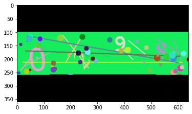
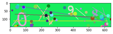
Figure 2.34: Sample of multicolor CAPTCHA dataset.

Chapter 3 Using Captcha-4-letter dataset (99.87 % accuracy)

3.1 Preprocessing

We have converted the raw images to binary images, i.e., which have only two values, 0 and 255 by performing adaptive thresholding as shown in Figure 3.1. When there is binary value, we can scale them down to 0 and 1 by dividing it with 255.0, so that the network is able to learn well from the data. This is one of the simplest types of CAPTCHA we have investigated with. The only challenge here is it has some connected letters which are hard to segment via any naive algorithm, so we have used a model to learn to predict all the letters at once. The data consists of about 9955 images of dimension 24x72x3. There is a total of 34 letters that are present in this CAPTCHA. Those letters includes all the capital letters and the digits.

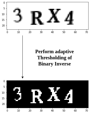
Figure 3.1: Performing adaptive thresholding of Binary Inverse before passing it to the model.

3.2 Naive Model for Captcha-4-letter dataset

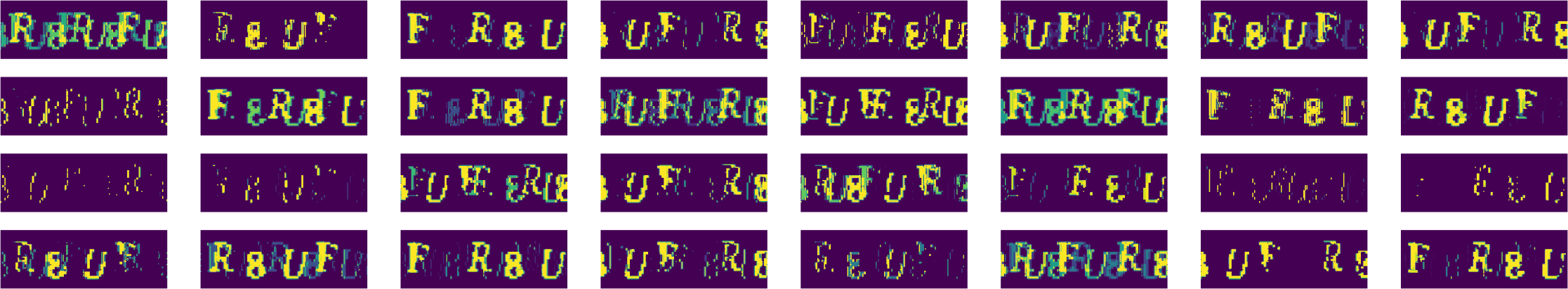
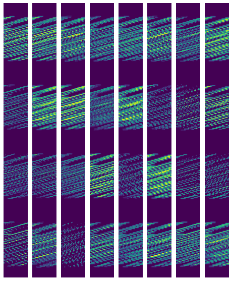
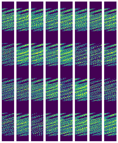
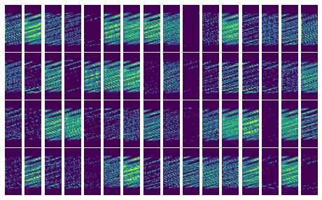
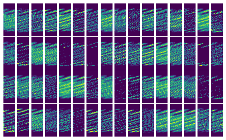
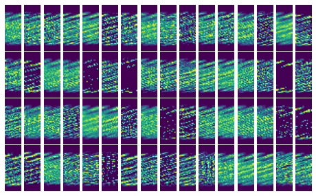
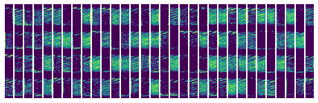
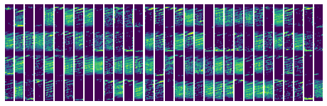
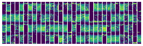
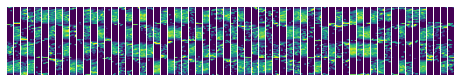
Figure 3.5: The visualizations of the features in a fully trained model when passed a CAPTCHA of FR8U, for Figure 3.4.

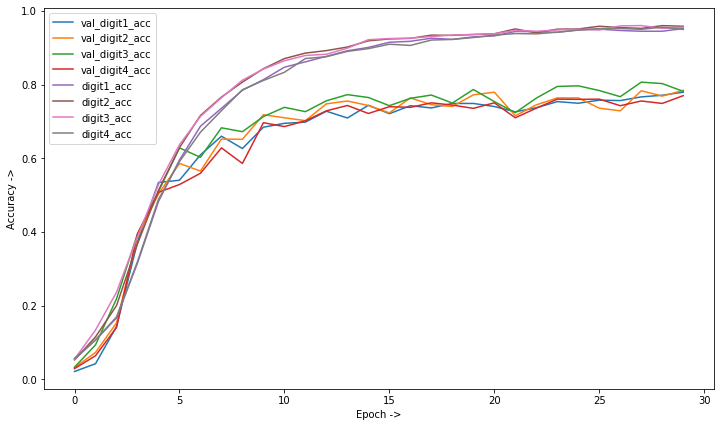
Figure 3.6: Plot for the training accuracy of our model.

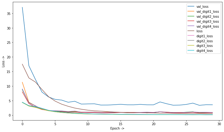
Figure 3.7: Plot for the training loss of our model.

The summary of the model is shown in Figure 3.2, which is generated by
$model.summary()$. The model is trained quite fast and after a total of 30 epochs, we get the accuracy of 77% as shown in Figure 3.3. It takes about 9 seconds per epochs and there are a total of 30 epochs, which takes about 4.5 minutes to train the whole dataset, which is pretty good. The intermediate graph of the model is shown in Figure 3.4. There is a total of 34 label so, this is a multi-label classification, we can see that the model has 4 outgoing nodes at the end for this task. The intermediate layers of the model that is learnt is shown in Figure 3.5. We first tried this naive model and the plots for the accuracy and the loss obtained from the model is shown in Figure 3.6 and Figure 3.7. After we have completed the training, we have tested on some random unseen data, and many were misclassified as shown in Figure 3.12. The trained model can be retrieved from this url (https://jimut123.github.io/blogs/CAPTCHA/models/captcha_4_letter_our_model.h5).

⬇

__________________________________________________________________________________________________

Layer (type) Output Shape Param # Connected to

==================================================

input_11 (InputLayer) (None, 200, 70, 1) 0

__________________________________________________________________________________________________

conv2d_71 (Conv2D) (None, 200, 70, 32) 320 input_11[0][0]

__________________________________________________________________________________________________

conv2d_72 (Conv2D) (None, 198, 68, 32) 9248 conv2d_71[0][0]

__________________________________________________________________________________________________

batch_normalization_36 (BatchNo (None, 198, 68, 32) 128 conv2d_72[0][0]

__________________________________________________________________________________________________

max_pooling2d_36 (MaxPooling2D) (None, 99, 34, 32) 0 batch_normalization_36[0][0]

__________________________________________________________________________________________________

dropout_35 (Dropout) (None, 99, 34, 32) 0 max_pooling2d_36[0][0]

__________________________________________________________________________________________________

conv2d_73 (Conv2D) (None, 99, 34, 64) 18496 dropout_35[0][0]

__________________________________________________________________________________________________

conv2d_74 (Conv2D) (None, 97, 32, 64) 36928 conv2d_73[0][0]

__________________________________________________________________________________________________

batch_normalization_37 (BatchNo (None, 97, 32, 64) 256 conv2d_74[0][0]

__________________________________________________________________________________________________

max_pooling2d_37 (MaxPooling2D) (None, 48, 16, 64) 0 batch_normalization_37[0][0]

__________________________________________________________________________________________________

dropout_36 (Dropout) (None, 48, 16, 64) 0 max_pooling2d_37[0][0]

__________________________________________________________________________________________________

conv2d_75 (Conv2D) (None, 48, 16, 128) 73856 dropout_36[0][0]

__________________________________________________________________________________________________

conv2d_76 (Conv2D) (None, 46, 14, 128) 147584 conv2d_75[0][0]

__________________________________________________________________________________________________

batch_normalization_38 (BatchNo (None, 46, 14, 128) 512 conv2d_76[0][0]

__________________________________________________________________________________________________

max_pooling2d_38 (MaxPooling2D) (None, 23, 7, 128) 0 batch_normalization_38[0][0]

__________________________________________________________________________________________________

dropout_37 (Dropout) (None, 23, 7, 128) 0 max_pooling2d_38[0][0]

__________________________________________________________________________________________________

conv2d_77 (Conv2D) (None, 21, 5, 256) 295168 dropout_37[0][0]

__________________________________________________________________________________________________

batch_normalization_39 (BatchNo (None, 21, 5, 256) 1024 conv2d_77[0][0]

__________________________________________________________________________________________________

max_pooling2d_39 (MaxPooling2D) (None, 10, 2, 256) 0 batch_normalization_39[0][0]

__________________________________________________________________________________________________

flatten_5 (Flatten) (None, 5120) 0 max_pooling2d_39[0][0]

__________________________________________________________________________________________________

dropout_38 (Dropout) (None, 5120) 0 flatten_5[0][0]

__________________________________________________________________________________________________

digit1 (Dense) (None, 34) 174114 dropout_38[0][0]

__________________________________________________________________________________________________

digit2 (Dense) (None, 34) 174114 dropout_38[0][0]

__________________________________________________________________________________________________

digit3 (Dense) (None, 34) 174114 dropout_38[0][0]

__________________________________________________________________________________________________

digit4 (Dense) (None, 34) 174114 dropout_38[0][0]

==================================================

Total params: 1,279,976

Trainable params: 1,279,016

Non-trainable params: 960

__________________________________________________________________________________________________

Figure 3.2: Summary of the model for 3.4.

⬇

Epoch 30/30

7200/7200 [==============================] - 9s 1ms/step - loss: 0.5274 - digit1_loss: 0.1373 - digit2_loss: 0.1242 - digit3_loss: 0.1226 - digit4_loss: 0.1434 - digit1_acc: 0.9519 - digit2_acc: 0.9583 - digit3_acc: 0.9558 - digit4_acc: 0.9497 - val_loss: 3.5470 - val_digit1_loss: 0.9227 - val_digit2_loss: 0.8700 - val_digit3_loss: 0.8337 - val_digit4_loss: 0.9206 - val_digit1_acc: 0.7794 - val_digit2_acc: 0.7844 - val_digit3_acc: 0.7817 - val_digit4_acc: 0.7700

Figure 3.3: The summary of 30 epochs for the model 3.4.

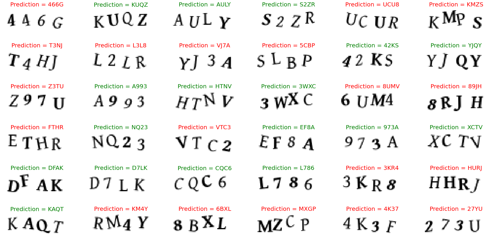
Figure 3.8: Prediction of the model on unseen data.

3.3 A better Model for Captcha-4-letter dataset

After a lot of fine tuning the hyperparameters, we found that we cannot improve much on the above model. We then came up with a new model as shown in Figure 3.9. The model took about 4.43 minutes in total of 38 epochs which gave an accuracy of 99.87% in total. There was careful design of TensorFlow callbacks which led to early stopping as shown in Figure 3.10. The graph of the same model is shown in Figure 3.11. The trained model can be retrieved from this url (https://jimut123.github.io/blogs/CAPTCHA/models/model_captcha_4_letter_v1.h5). We test the accuracy of the model on some real-world unseen data as shown in Figure 3.12, which shows that it operates in a human level accuracy with all of the predictions correct. The loss of the model is shown in Figure 3.13.

⬇

__________________________________________________________________________________________________

Layer (type) Output Shape Param # Connected to

==================================================

input_data (InputLayer) (None, 72, 24, 1) 0

__________________________________________________________________________________________________

Conv1 (Conv2D) (None, 72, 24, 32) 320 input_data[0][0]

__________________________________________________________________________________________________

pool1 (MaxPooling2D) (None, 36, 12, 32) 0 Conv1[0][0]

__________________________________________________________________________________________________

Conv2 (Conv2D) (None, 36, 12, 64) 18496 pool1[0][0]

__________________________________________________________________________________________________

pool2 (MaxPooling2D) (None, 18, 6, 64) 0 Conv2[0][0]

__________________________________________________________________________________________________

reshape (Reshape) (None, 18, 384) 0 pool2[0][0]

__________________________________________________________________________________________________

dense1 (Dense) (None, 18, 64) 24640 reshape[0][0]

__________________________________________________________________________________________________

bi_1 (Bidirectional) (None, 18, 256) 198656 dense1[0][0]

__________________________________________________________________________________________________

bi_2 (Bidirectional) (None, 18, 256) 395264 bi_1[0][0]

__________________________________________________________________________________________________

dense2 (Dense) (None, 18, 33) 8481 bi_2[0][0]

__________________________________________________________________________________________________

input_label (InputLayer) (None, 4) 0

__________________________________________________________________________________________________

input_length (InputLayer) (None, 1) 0

__________________________________________________________________________________________________

label_length (InputLayer) (None, 1) 0

__________________________________________________________________________________________________

ctc_loss (Lambda) (None, 1) 0 dense2[0][0]

input_label[0][0]

input_length[0][0]

label_length[0][0]

==================================================

Total params: 645,857

Trainable params: 645,857

Non-trainable params: 0

__________________________________________________________________________________________________

Figure 3.9: Summary of the Version 2 of the Model

⬇

Epoch 38/50

279/279 [==============================] - 7s 26ms/step - loss: 0.1842 - val_loss: 0.1233

Figure 3.10: The epochs for version 2 of the model.

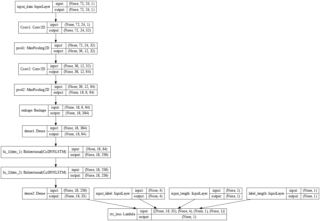
Figure 3.11: Version 2 of the model for identifying individual characters.

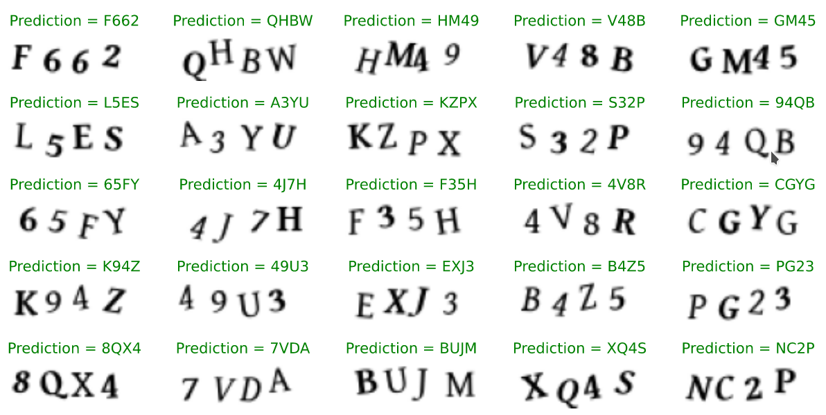
Figure 3.12: Prediction of the new model (3.11) on unseen data.

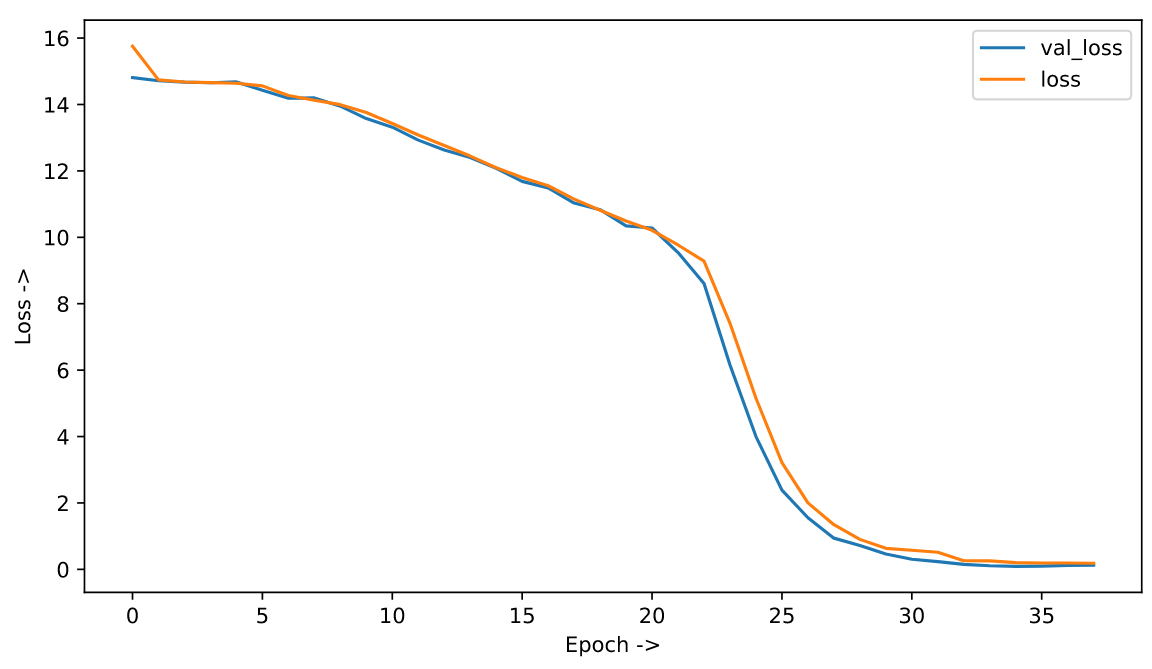
Figure 3.13: Loss of the new model (3.11).

In Figure 3.14 we see the 3x3 kernels that are being learned by the layer 1 of the network for the Model 3.11. The visualization of the weights learned by the same model can be seen in Figure 3.15.

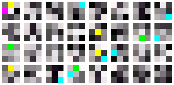
Figure 3.14: The 3x3 kernels (filter) learned by the model (3.11) for layer 1.

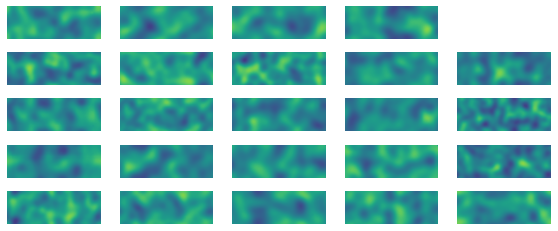
Figure 3.15: The weights learned by the model (3.11) for layers 1 to 24.

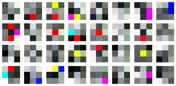
Figure 3.16: The 3x3 kernels (filter) learned by the model (7.5) for layer 1.

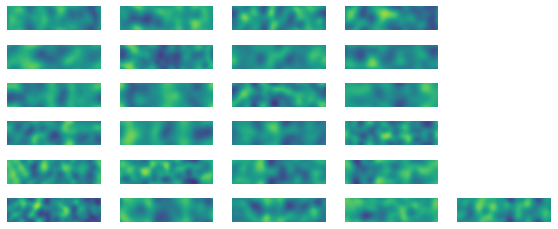
Figure 3.17: The weights learned by the model (7.5) for layers 1 to 26.

Chapter 4 Using c4l_16x16_550 dataset (99.91 % accuracy)

4.1 Model for c4l_16x16_550 dataset

We have used a modified version of CIFAR 10 like model for predicting the segmented images. The summary of the architecture of the model is shown below

⬇

_________________________________________________________________

Layer (type) Output Shape Param #

=================================================================

conv2d_1 (Conv2D) (None, 16, 16, 32) 320

_________________________________________________________________

activation_1 (Activation) (None, 16, 16, 32) 0

_________________________________________________________________

conv2d_2 (Conv2D) (None, 14, 14, 32) 9248

_________________________________________________________________

activation_2 (Activation) (None, 14, 14, 32) 0

_________________________________________________________________

max_pooling2d_1 (MaxPooling2 (None, 7, 7, 32) 0

_________________________________________________________________

dropout_1 (Dropout) (None, 7, 7, 32) 0

_________________________________________________________________

conv2d_3 (Conv2D) (None, 7, 7, 64) 18496

_________________________________________________________________

activation_3 (Activation) (None, 7, 7, 64) 0

_________________________________________________________________

conv2d_4 (Conv2D) (None, 5, 5, 64) 36928

_________________________________________________________________

activation_4 (Activation) (None, 5, 5, 64) 0

_________________________________________________________________

max_pooling2d_2 (MaxPooling2 (None, 2, 2, 64) 0

_________________________________________________________________

dropout_2 (Dropout) (None, 2, 2, 64) 0

_________________________________________________________________

flatten_1 (Flatten) (None, 256) 0

_________________________________________________________________

dense_1 (Dense) (None, 512) 131584

_________________________________________________________________

activation_5 (Activation) (None, 512) 0

_________________________________________________________________

dropout_3 (Dropout) (None, 512) 0

_________________________________________________________________

dense_2 (Dense) (None, 32) 16416

_________________________________________________________________

activation_6 (Activation) (None, 32) 0

=================================================================

Total params: 212,992

Trainable params: 212,992

Non-trainable params: 0

_________________________________________________________________

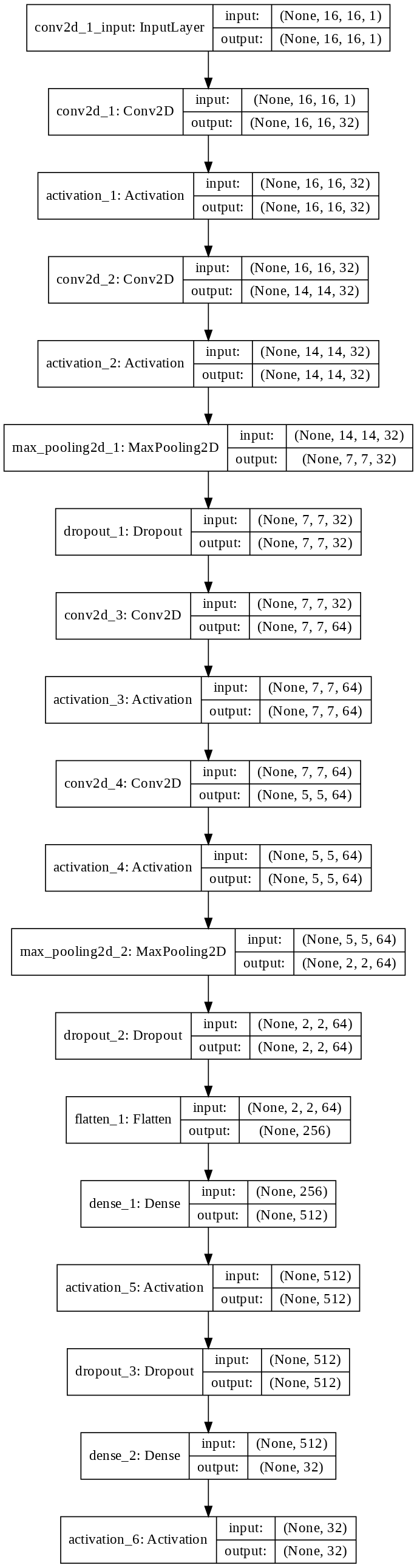
Figure 4.1: CIFAR 10 like model for identifying individual characters.

After about 20 epochs, we got an accuracy of 99.91 % on the validation split. We find that the training of the individual split characters is very fast due to its small size and uniform distribution. It took a total of about 0.6 minutes to train on the whole dataset. We further note that the accuracy is beyond the model used in Figure 3.11. This operates in human level accuracy. It might be due to overfitting but this works well in general.

⬇

Epoch 20/20

14105/14105 [==============================] - 2s 172us/step - loss: 0.0257 - acc: 0.9950 - val_loss: 0.0140 - val_acc: 0.9991

Figure 4.2: epochs.

The visualization of the architecture of the model is shown in Figure  4.1.

The graph of the accuracy of the model is shown in Figure  4.3 and the loss of the model is shown in Figure  4.4. The trained model can be retrieved from this url (https://jimut123.github.io/blogs/CAPTCHA/models/CNN_c4l-16x16_550.h5).

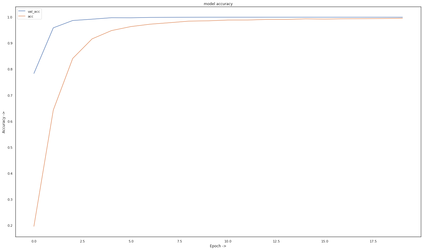
Figure 4.3: Accuracy of the model as shown in Figure  4.1

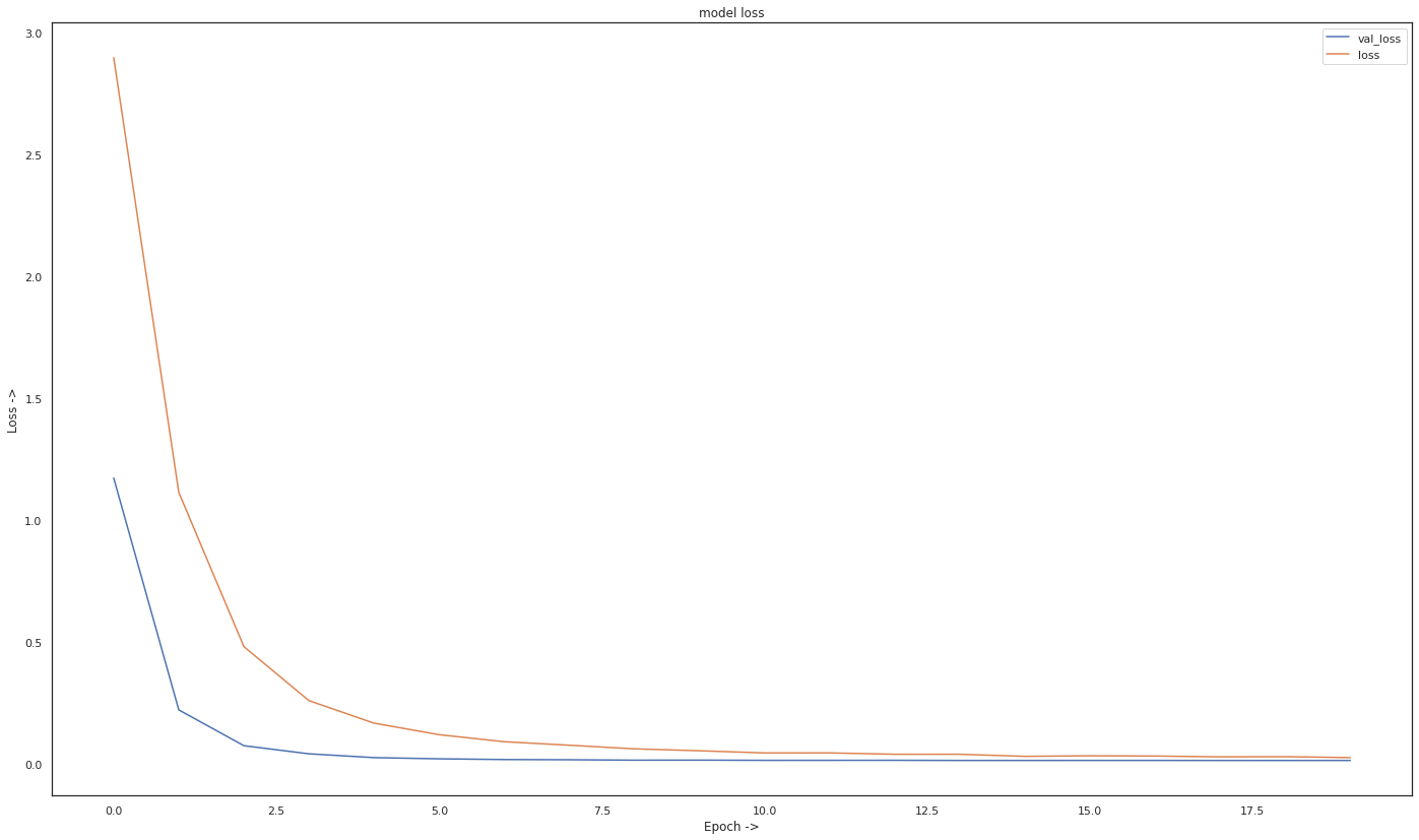
Figure 4.4: Accuracy of the model as shown in Figure  4.1

We can see that the prediction of the model on individual character is almost with 100% accuracy as shown in Figure 4.5.

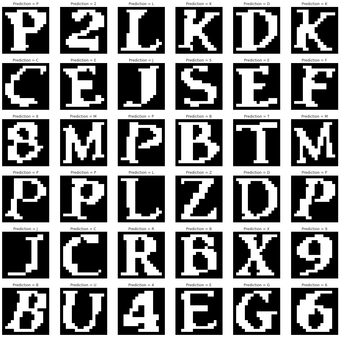
Figure 4.5: The prediction of the model from the individual characters

The confusion matrix for individual character predicted is shown in Figure 4.6.

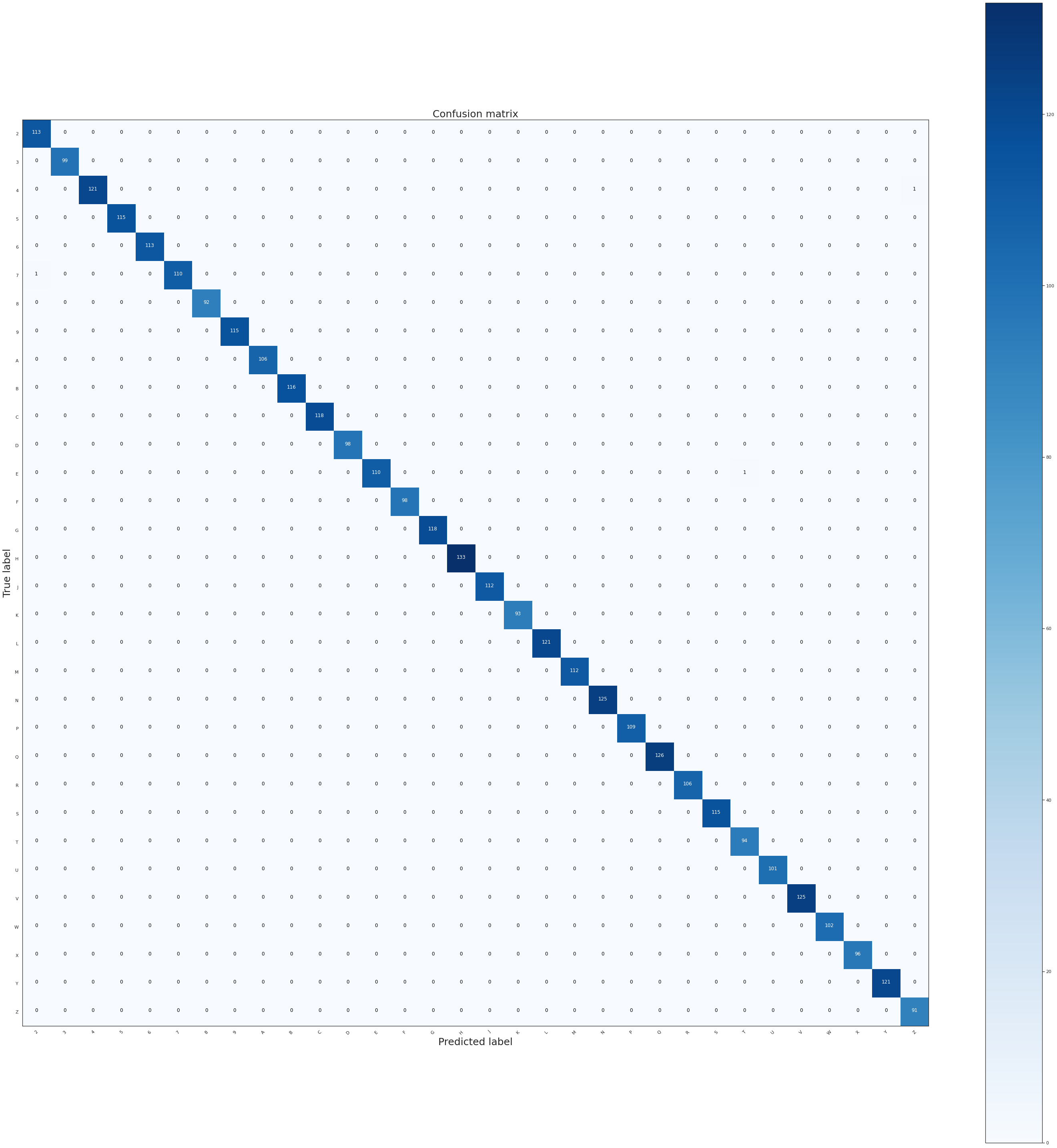
Figure 4.6: The confusion matrix of the individual characters

Visualizations generated from the layers of convolutional neural network when passed the images of character 2, L, K and P are shown in Figures 4.7, 4.8, 4.9 and 4.10. These are the intermediate visualizations generated to finally arrive at the last layer of fully connected layer to determine which letter it actually belongs to.

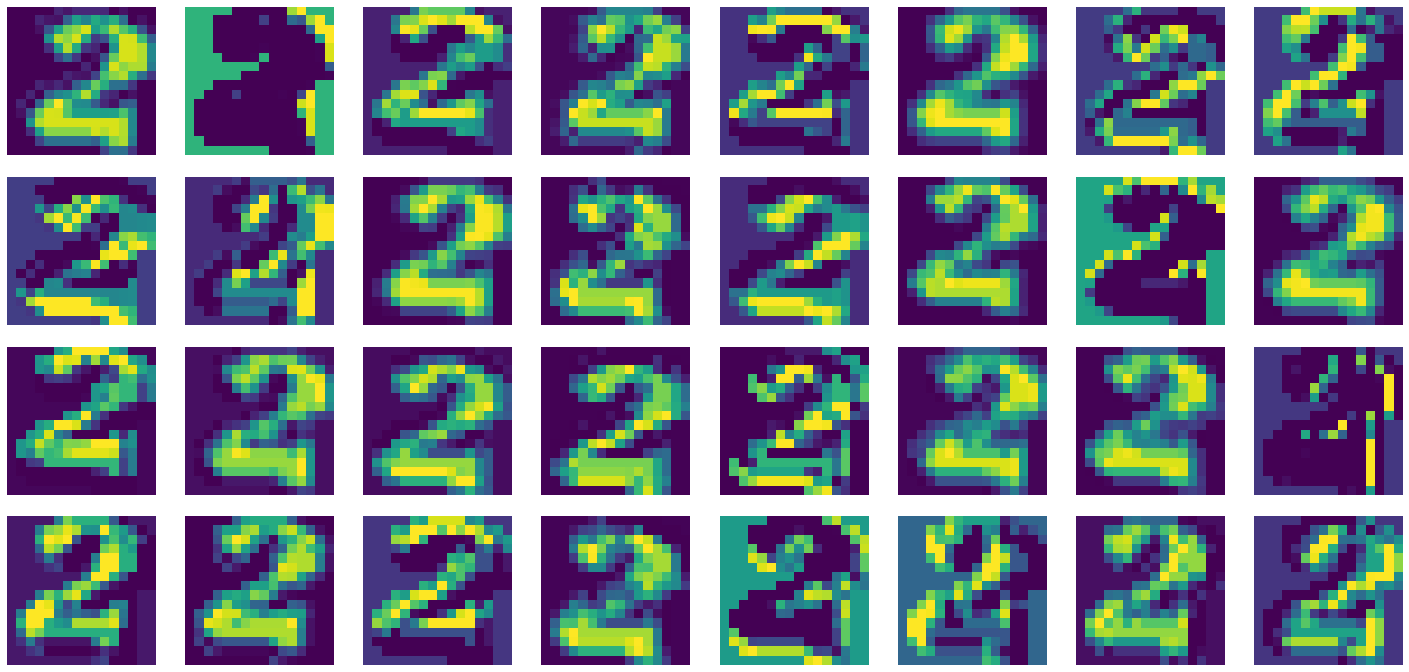
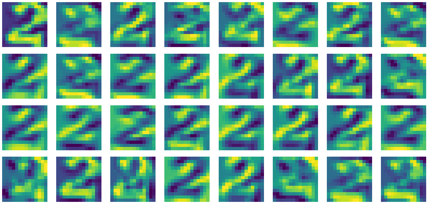
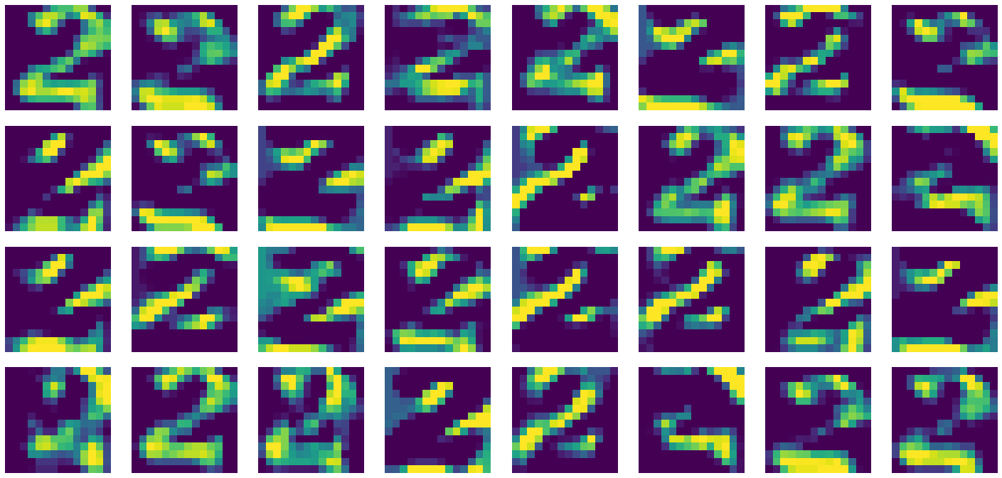
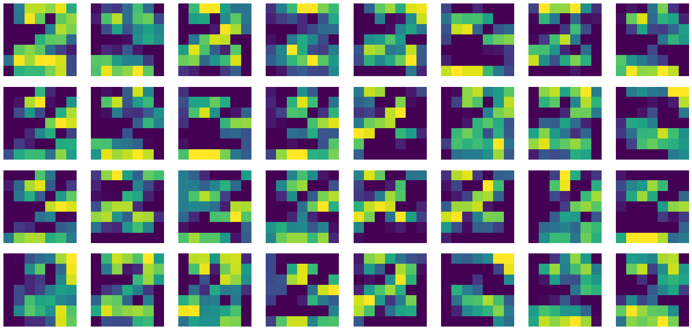
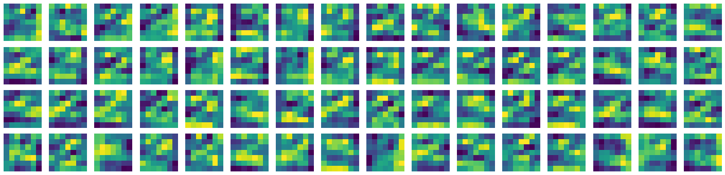
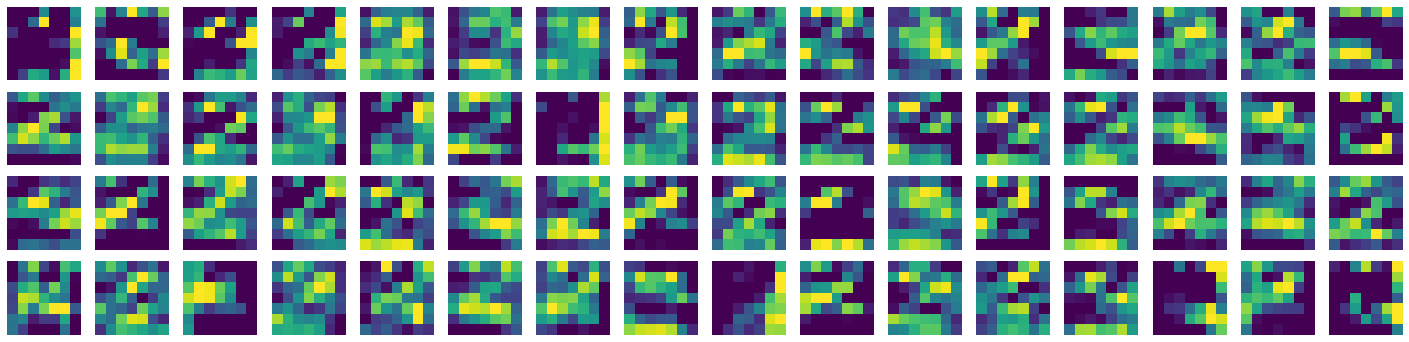
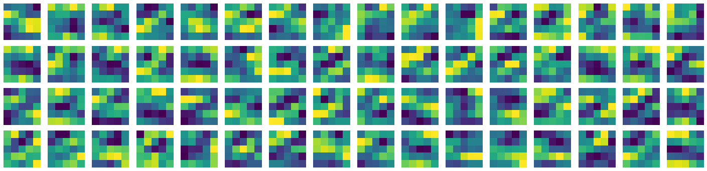
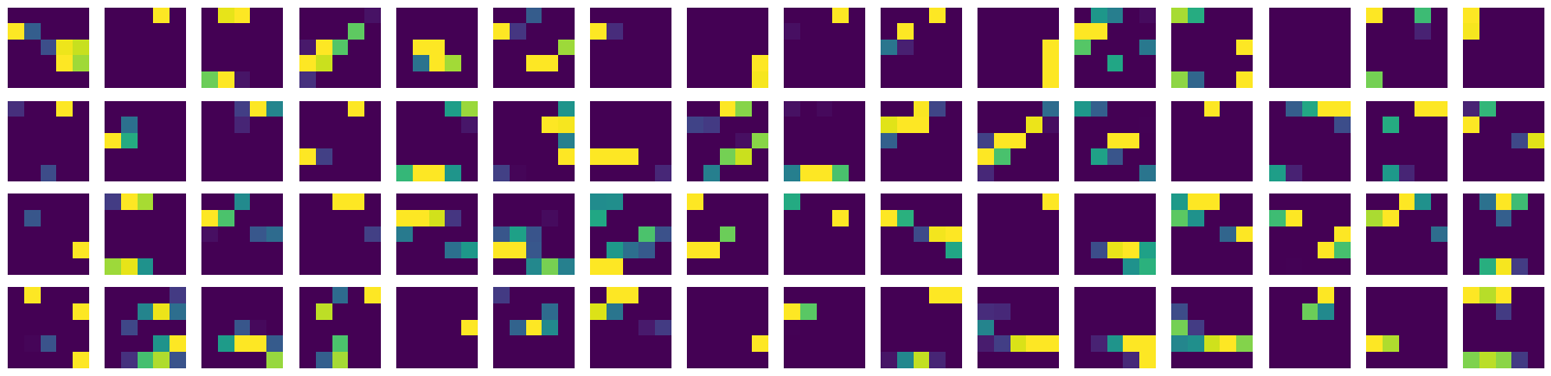
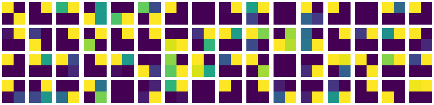
Figure 4.7: The visualizations of the features in a fully trained model when passed an image for letter 2.

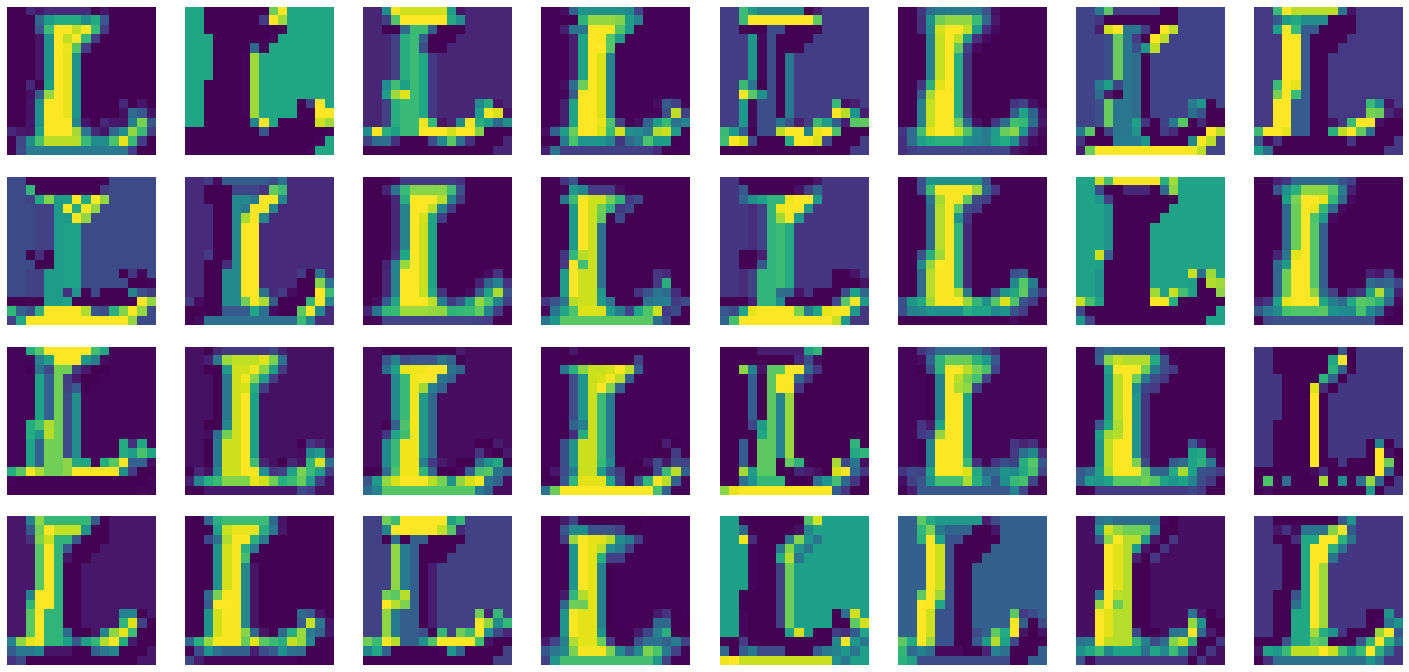
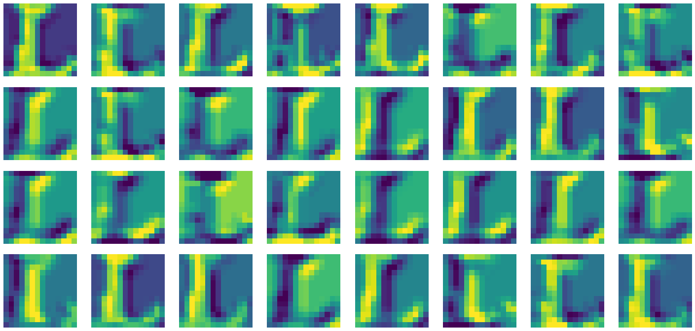
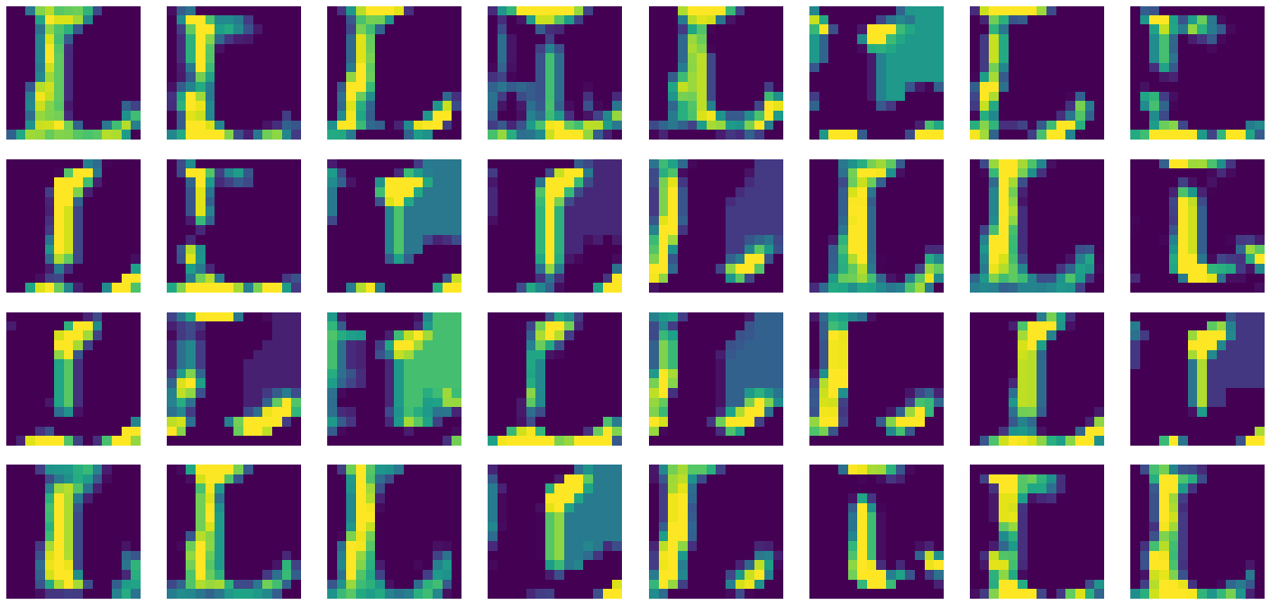
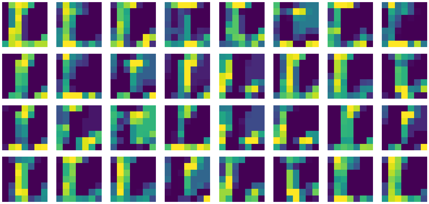
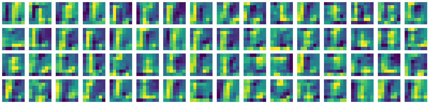
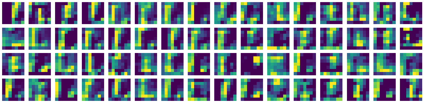
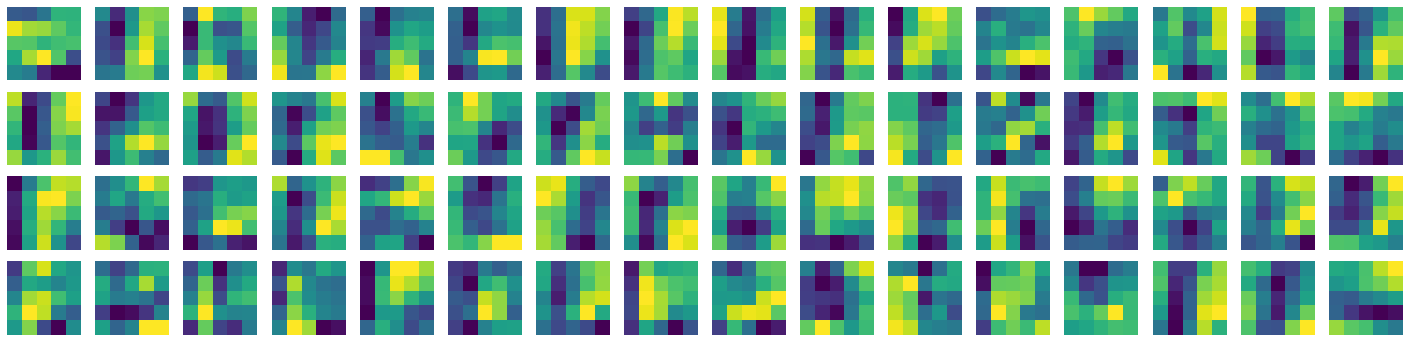
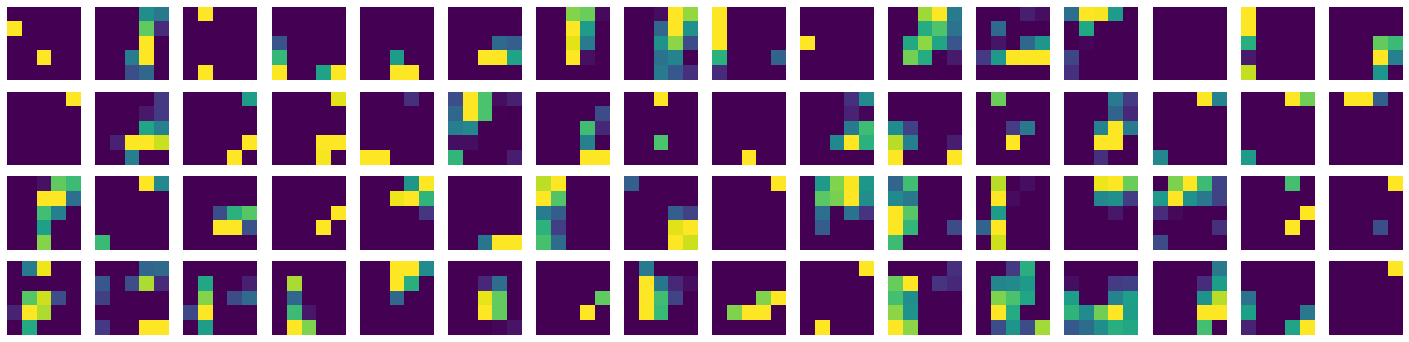
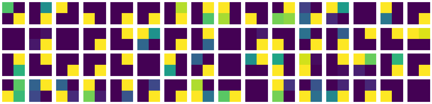
Figure 4.8: The visualizations of the features in a fully trained model when passed an image for letter L.

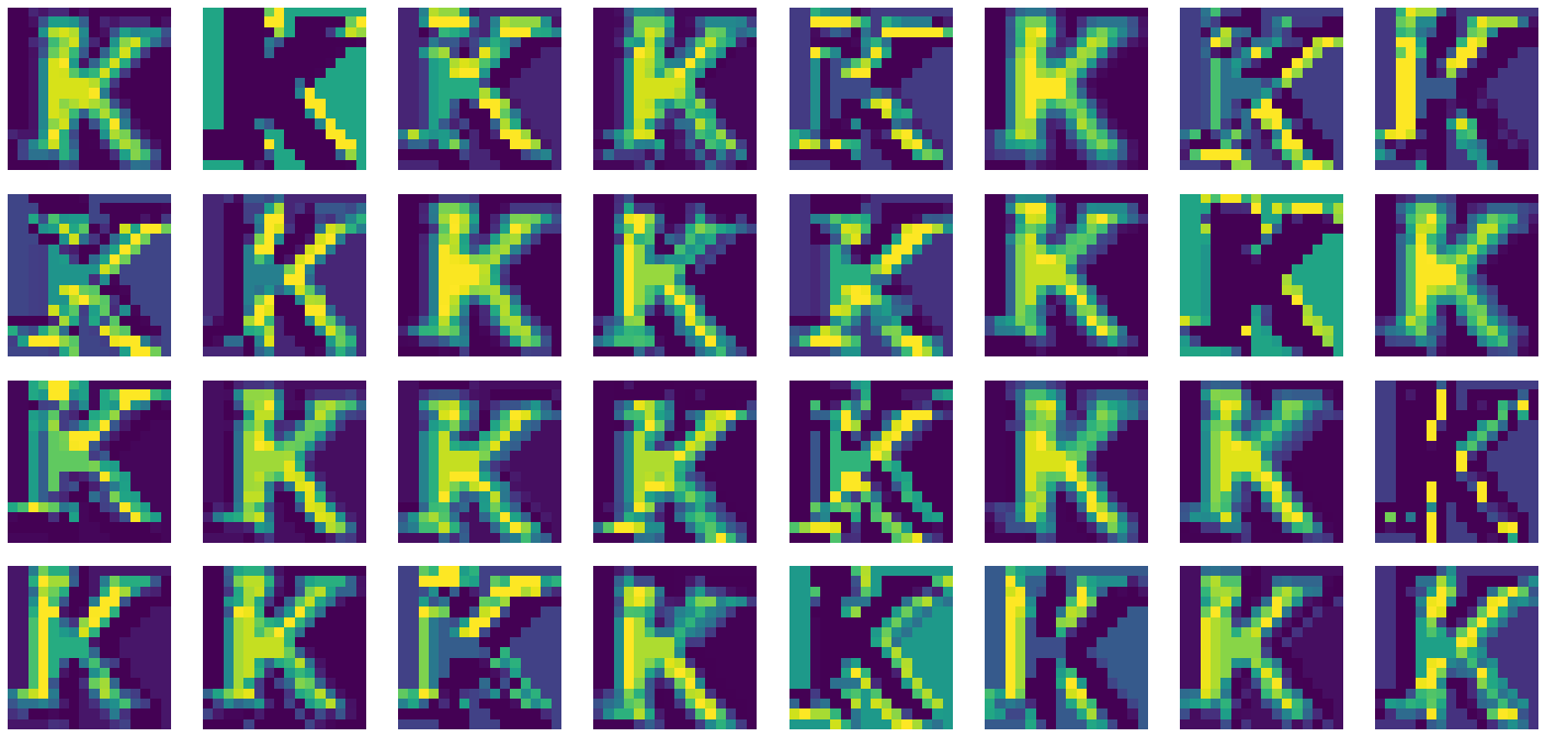
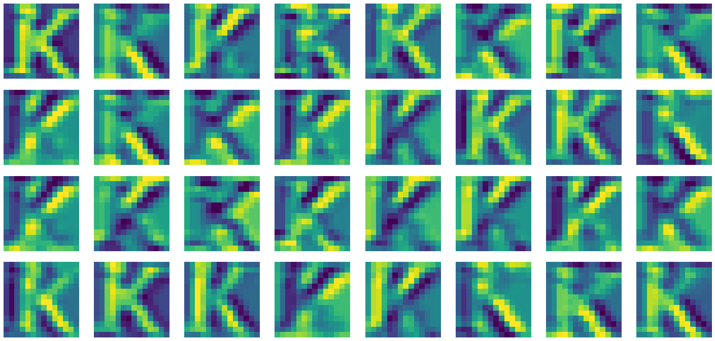
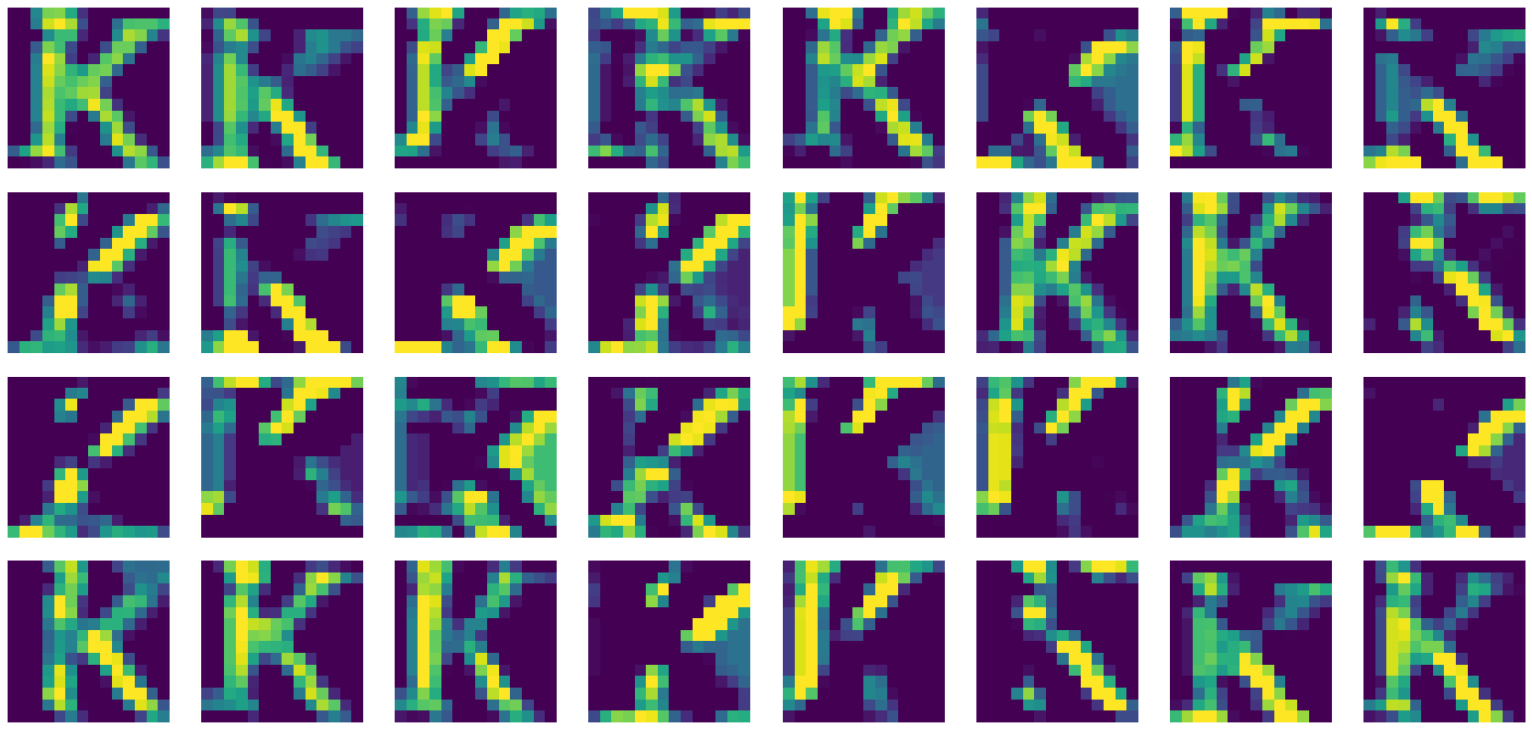
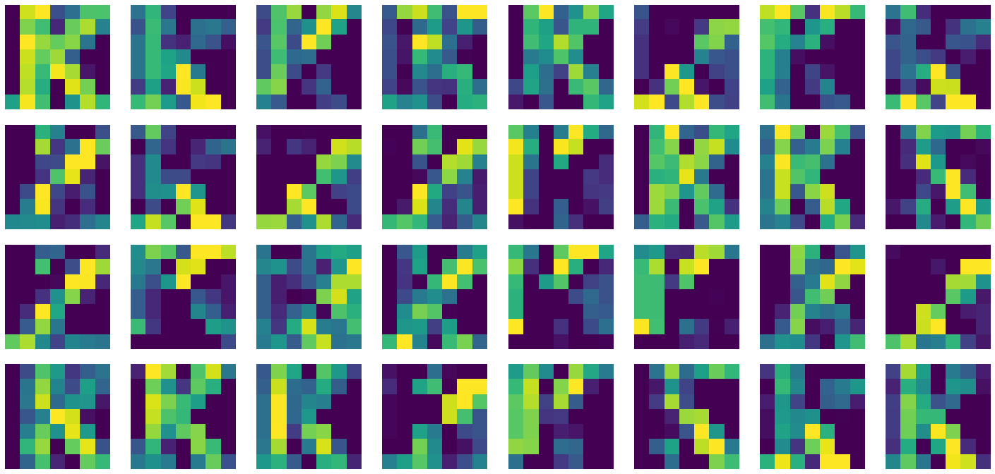
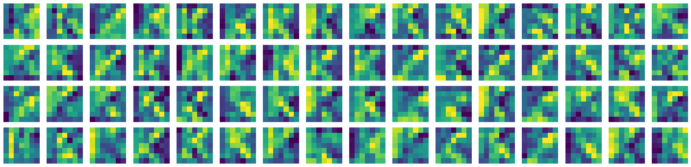
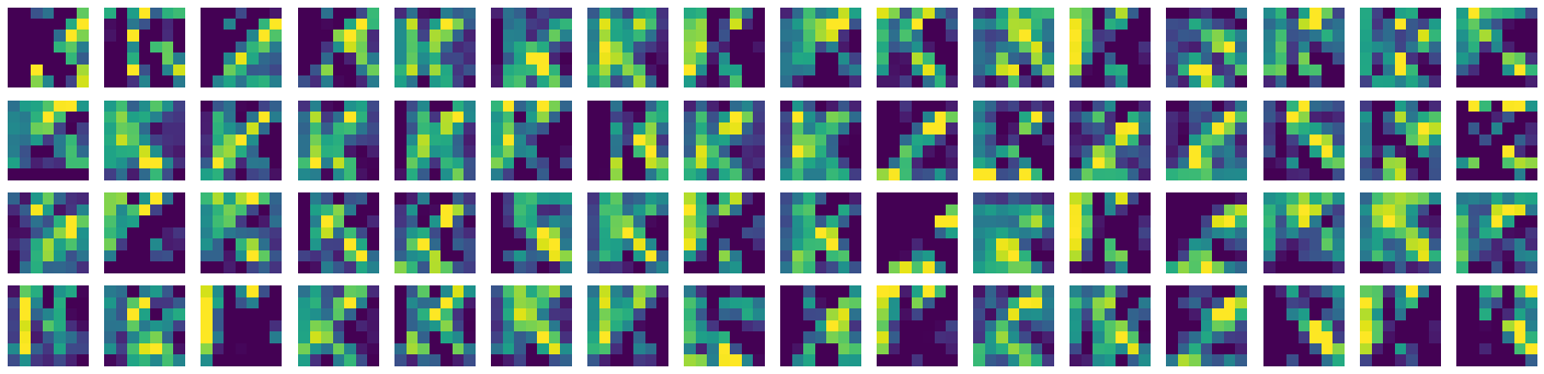
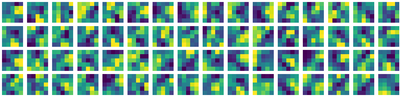
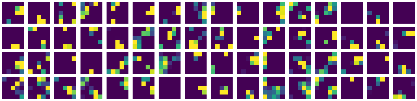
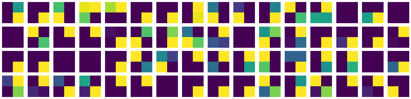
Figure 4.9: The visualizations of the features in a fully trained model when passed an image for letter K.

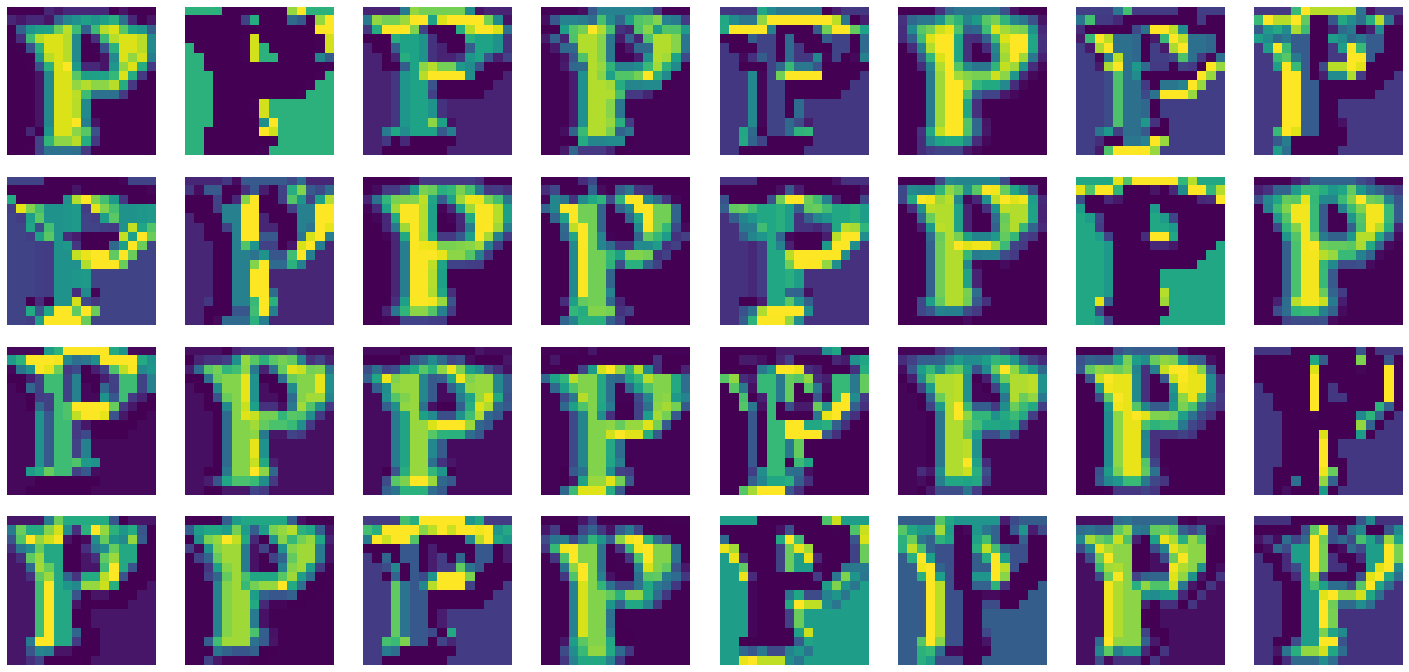
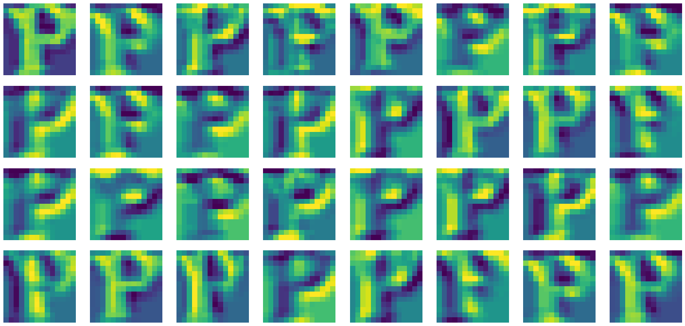
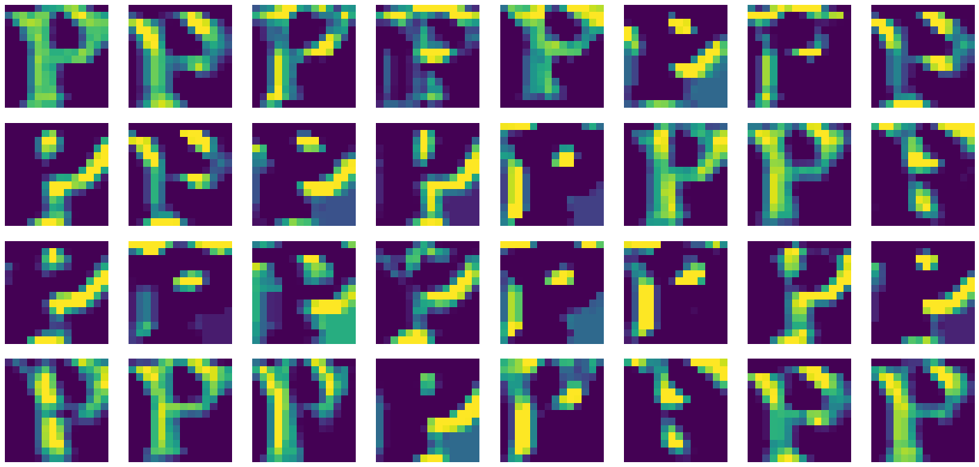
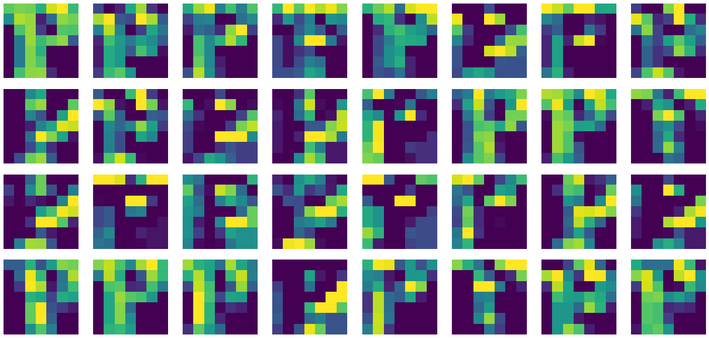
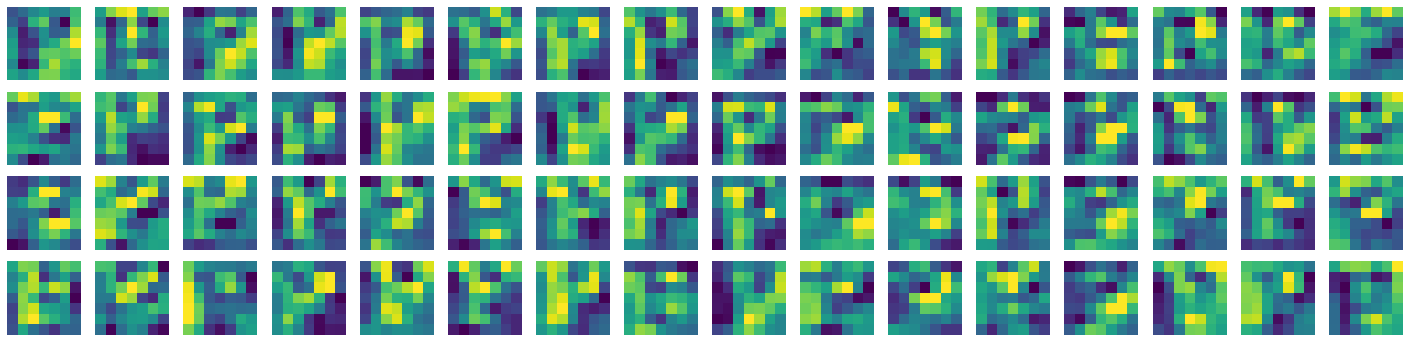
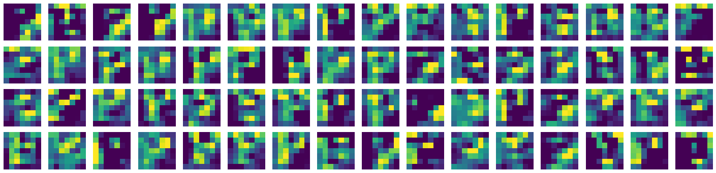
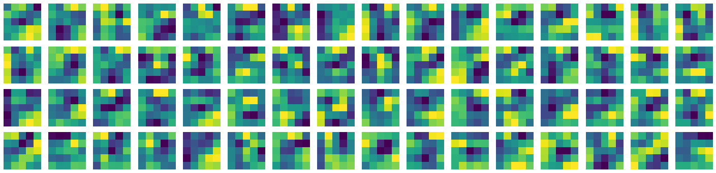
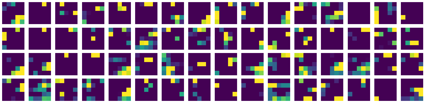
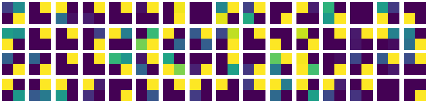
Figure 4.10: The visualizations of the features in a fully trained model when passed an image for letter P.

4.2 When using on real unseen data

When the model was downloaded from Google Collaboratory to local machine, it was tested on a sample of about 100 images, of which 96 were correctly classified, except these four images as shown in Figure 4.11.

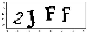
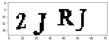
2JFF classified as 2AFF                   2JRJ classified as 2KRJ

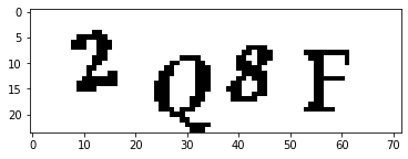
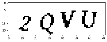
2Q8F classified as 2A8F                   2QVU classified as 2JVU

Figure 4.11: The wrong classification of the model.

After testing on 100 unseen CAPTCHA images, we found that these four were incorrectly labelled as shown in Figure 4.11. This is good since we are getting the validation accuracy on individual characters and it somehow mislabells J as F and K, Q as J and and A. The accuracy on individual character will be 99.99% which is great.

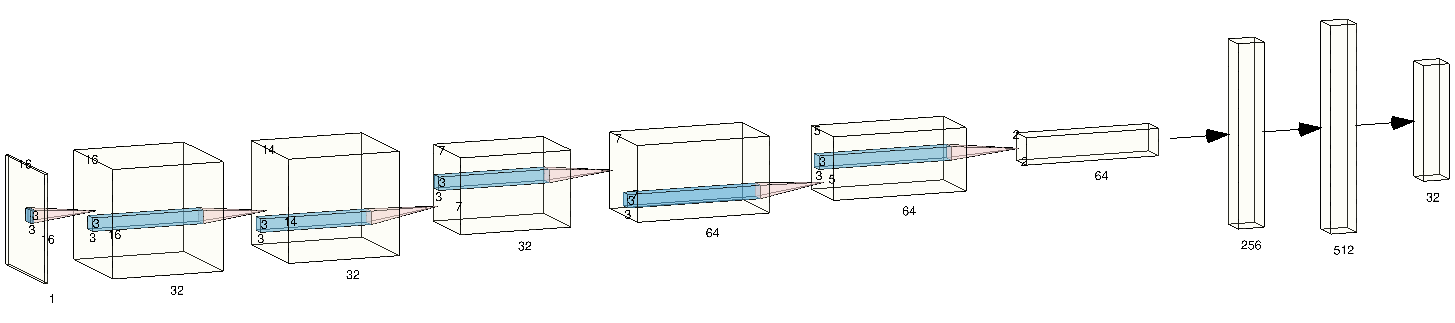
Figure 4.12: The Alex net type architecture. Created using https://alexlenail.me/NN-SVG/.

In Figure 4.13 we see the 3x3 kernels that are being learned by the layer 1 of the network for the Model 4.1. The visualization of the weights learned by the same model can be seen in Figure 4.14.

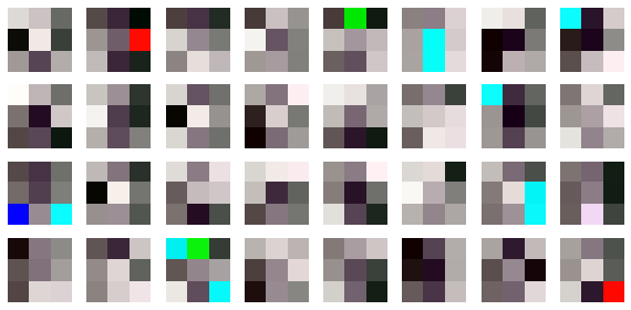
Figure 4.13: The 3x3 kernels (filter) learned by the model (4.1) for layer 1.

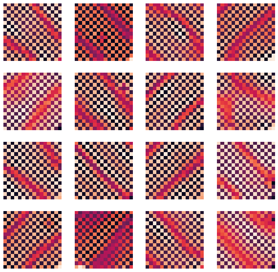
Figure 4.14: The weights learned by the model (4.1) for layers 1 to 16.

Chapter 5 Using resized_JAM CAPTCHAs dataset to predict JAM data (99.53 % accuracy)

5.1 Using k-NN for resized_JAM CAPTCHA dataset

We used the $k$-Nearest Neighbor (k-NN) algorithm for prediction of resized_JAM dataset. Using a $k$ of value $7$ we got 99.53% testing accuracy, which is almost state of the art. We varied the value of $k$ to get the best accuracy as shown in Figure 5.1. The confusion matrix for the same is shown in Figure 5.2. The only confusion here is 9 is misclassified as 5 in some data which might be due to noise. This shows that even a simple and computationally efficient model (when the data is less), can give a high accuracy which is almost the state of the art.

This even shows that the IITK JAM website needs a better version of CAPTCHA since this is very easy to break using KNN. When there are choices whether to choose a complex model or a simple model, people should choose a simple model which gives accuracy comparable to the complex model.

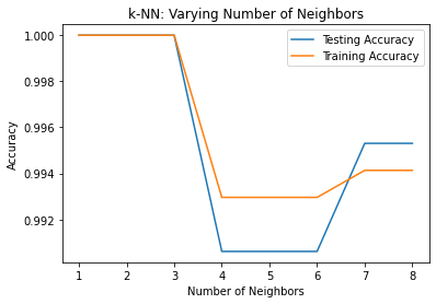
Figure 5.1: Varying the value of $k$ to get the best testing accuracy.

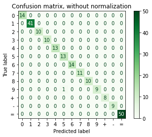
Figure 5.2: The confusion matrix of the resized_JAM dataset.

Chapter 6 Using CAPTCHA-version-2 dataset (90.102 % accuracy)

6.1 Using AlexNet type Model

The sample images of CAPTCHA-version-2 dataset is shown in Figure 2.20. It is clear that there is a great challenge in classifying the labels of such a dataset. The main reason is presence of certain amount of noise in the dataset in terms of clutter and scratch. Firstly, we used an Alex Net type model as shown in Figure 6.4. We trained about 30 epochs and each epoch took about 1 second. This means it took 30 second to complete the whole training, which is pretty fast. The model used is similar to 8.1, which can detect even those CAPTCHAs which are occluded by noise. The loss and accuracy for the training is shown in Figure 6.2 and Figure 6.1 respectively. The accuracy obtained during training was about 97.87% and the accuracy obtained during testing was about 76.54 % which was pretty useless. The summary of the epochs can be found in Figure 6.5. The model can be found from this url (https://jimut123.github.io/blogs/CAPTCHA/models/captcha_v2_alexNet.h5).

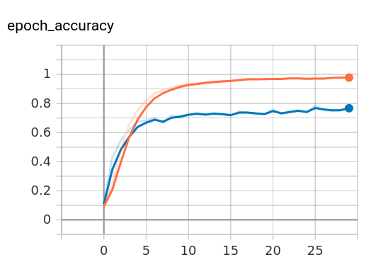
Figure 6.1: Accuracy obtained from the AlexNet type model (8.1).

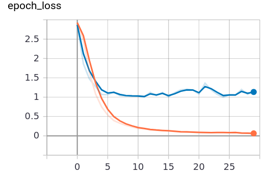
Figure 6.2: Loss obtained from the AlexNet type model (8.1).

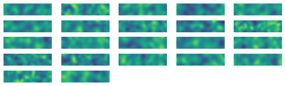
Figure 6.3: The weights learned by the model (8.1) for layers 1 to 16.

⬇

_________________________________________________________________

Layer (type) Output Shape Param #

==================================================

input_1 (InputLayer) [(None, 50, 200, 1)] 0

_________________________________________________________________

conv2d (Conv2D) (None, 48, 198, 32) 320

_________________________________________________________________

max_pooling2d (MaxPooling2D) (None, 24, 99, 32) 0

_________________________________________________________________

conv2d_1 (Conv2D) (None, 22, 97, 64) 18496

_________________________________________________________________

max_pooling2d_1 (MaxPooling2 (None, 11, 48, 64) 0

_________________________________________________________________

conv2d_2 (Conv2D) (None, 9, 46, 64) 36928

_________________________________________________________________

max_pooling2d_2 (MaxPooling2 (None, 4, 23, 64) 0

_________________________________________________________________

flatten (Flatten) (None, 5888) 0

_________________________________________________________________

dense (Dense) (None, 1024) 6030336

_________________________________________________________________

dropout (Dropout) (None, 1024) 0

_________________________________________________________________

dense_1 (Dense) (None, 95) 97375

_________________________________________________________________

reshape (Reshape) (None, 5, 19) 0

==================================================

Total params: 6,183,455

Trainable params: 6,183,455

Non-trainable params: 0

_________________________________________________________________

Figure 6.4: Summary of the AlexNet type model for classifying the labels of CAPTCHA-version-2 dataset.

⬇

Epoch 30/30

120/120 [==============================] - 1s 12ms/step - loss: 0.0613 - accuracy: 0.9787 - val_loss: 1.1524 - val_accuracy: 0.7750

Figure 6.5: Summary of epochs for the model (6.4).

Figure 6.6: The weights learned by the model (6.12) for layers 1 to 16.

6.2 Using a better Model

⬇

__________________________________________________________________________________________________

Layer (type) Output Shape Param # Connected to

==================================================

input_1 (InputLayer) (None, 50, 200, 1) 0

__________________________________________________________________________________________________

conv2d_1 (Conv2D) (None, 50, 200, 16) 160 input_1[0][0]

__________________________________________________________________________________________________

max_pooling2d_1 (MaxPooling2D) (None, 25, 100, 16) 0 conv2d_1[0][0]

__________________________________________________________________________________________________

conv2d_2 (Conv2D) (None, 25, 100, 32) 4640 max_pooling2d_1[0][0]

__________________________________________________________________________________________________

max_pooling2d_2 (MaxPooling2D) (None, 13, 50, 32) 0 conv2d_2[0][0]

__________________________________________________________________________________________________

conv2d_3 (Conv2D) (None, 13, 50, 32) 9248 max_pooling2d_2[0][0]

__________________________________________________________________________________________________

batch_normalization_1 (BatchNor (None, 13, 50, 32) 128 conv2d_3[0][0]

__________________________________________________________________________________________________

max_pooling2d_3 (MaxPooling2D) (None, 7, 25, 32) 0 batch_normalization_1[0][0]

__________________________________________________________________________________________________

flatten_1 (Flatten) (None, 5600) 0 max_pooling2d_3[0][0]

__________________________________________________________________________________________________

dense_1 (Dense) (None, 64) 358464 flatten_1[0][0]

__________________________________________________________________________________________________

dense_3 (Dense) (None, 64) 358464 flatten_1[0][0]

__________________________________________________________________________________________________

dense_5 (Dense) (None, 64) 358464 flatten_1[0][0]

__________________________________________________________________________________________________

dense_7 (Dense) (None, 64) 358464 flatten_1[0][0]

__________________________________________________________________________________________________

dense_9 (Dense) (None, 64) 358464 flatten_1[0][0]

__________________________________________________________________________________________________

dropout_1 (Dropout) (None, 64) 0 dense_1[0][0]

__________________________________________________________________________________________________

dropout_2 (Dropout) (None, 64) 0 dense_3[0][0]

__________________________________________________________________________________________________

dropout_3 (Dropout) (None, 64) 0 dense_5[0][0]

__________________________________________________________________________________________________

dropout_4 (Dropout) (None, 64) 0 dense_7[0][0]

__________________________________________________________________________________________________

dropout_5 (Dropout) (None, 64) 0 dense_9[0][0]

__________________________________________________________________________________________________

dense_2 (Dense) (None, 36) 2340 dropout_1[0][0]

__________________________________________________________________________________________________

dense_4 (Dense) (None, 36) 2340 dropout_2[0][0]

__________________________________________________________________________________________________

dense_6 (Dense) (None, 36) 2340 dropout_3[0][0]

__________________________________________________________________________________________________

dense_8 (Dense) (None, 36) 2340 dropout_4[0][0]

__________________________________________________________________________________________________

dense_10 (Dense) (None, 36) 2340 dropout_5[0][0]

==================================================

Total params: 1,818,196

Trainable params: 1,818,132

Non-trainable params: 64

__________________________________________________________________________________________________

Figure 6.7: Summary of the model for classifying the labels of CAPTCHA-version-2 dataset.

Figure 6.8: Model for training CAPTCHA-version-2 dataset.

⬇

Epoch 30/30

776/776 [==============================] - 1s 693us/step - loss: 1.2762 - dense_2_loss: 0.1197 - dense_4_loss: 0.1451 - dense_6_loss: 0.3858 - dense_8_loss: 0.3225 - dense_10_loss: 0.3031 - dense_2_acc: 0.9601 - dense_4_acc: 0.9549 - dense_6_acc: 0.8389 - dense_8_acc: 0.8802 - dense_10_acc: 0.8892 - val_loss: 2.0466 - val_dense_2_loss: 0.0376 - val_dense_4_loss: 0.2783 - val_dense_6_loss: 0.4414 - val_dense_8_loss: 0.8160 - val_dense_10_loss: 0.4733 - val_dense_2_acc: 0.9897 - val_dense_4_acc: 0.9433 - val_dense_6_acc: 0.8608 - val_dense_8_acc: 0.8299 - val_dense_10_acc: 0.8814

Figure 6.9: Summary of epochs for the model (6.8).

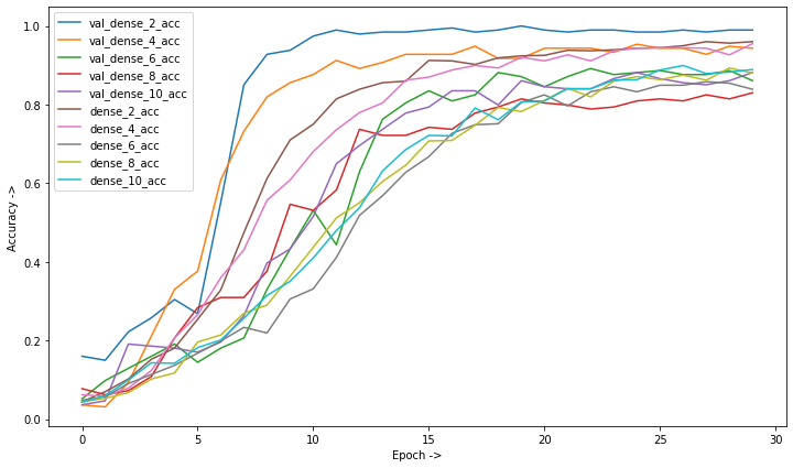
Figure 6.10: Accuracy of the model (6.8).

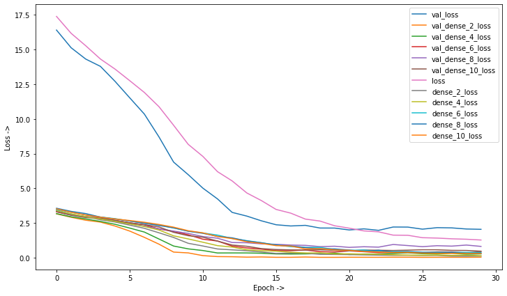
Figure 6.11: Loss of the model (6.8).

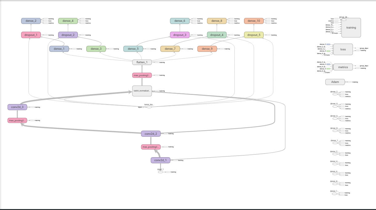
Figure 6.12: Tensorboard Visualization of the structure of the model (6.8).

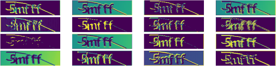
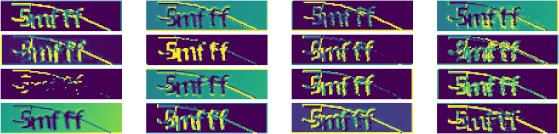
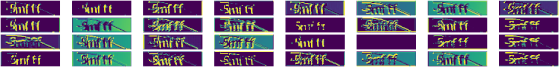
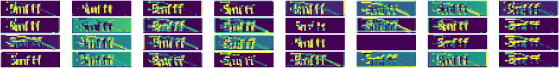
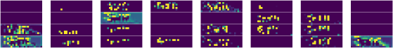
Figure 6.13: The visualizations of the features in a fully trained model for Model 6.12 when passed a CAPTCHA containing the text 5mfff.

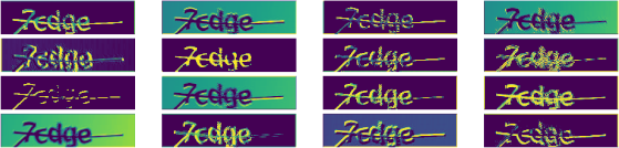
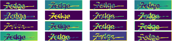
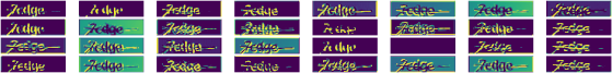
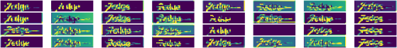
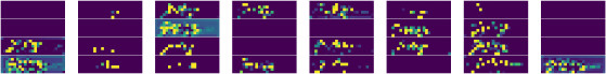
Figure 6.14: The visualizations of the features in a fully trained model for Model 6.12 when passed a CAPTCHA containing the text 7cdge.

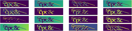
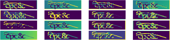
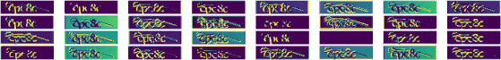
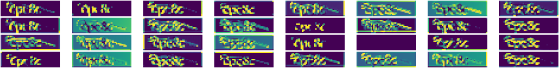
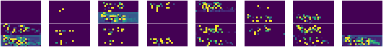
Figure 6.15: The visualizations of the features in a fully trained model for Model 6.12 when passed a CAPTCHA containing the text cpc8c.

In Figure 6.16 we see the 3x3 kernels that are being learned by the layer 1 of the network for the Model 6.12. The visualization of the weights learned by the same model can be seen in Figure 6.6.

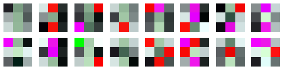
Figure 6.16: The 3x3 kernels (filter) learned by the model (6.12) for layer 1.

The summary of the structure of the model is shown in Figure 6.7. The graph diagram of the model is shown in Figure 6.8. The trained model can be retrieved from this url (https://jimut123.github.io/blogs/CAPTCHA/models/captcha_v2_1_drive.h5). This is clear that it is a multi-label classification which classifies 36 labels including the lower-case ASCII alphabets (a-z) and the number of digits from 0-9. The model was trained in 30 epochs, the final epochs’ summary is shown in Figure 6.9. It took about 1 second per epochs after the first epoch which took 8 second. The total training time of the model was about 38 seconds which is pretty fast.

The graph of the accuracy and the loss are shown in Figure 6.10 and 6.11. The tensor board visualization of the model graph is shown in Figure 6.12. The intermediate visualization of the convolution layer when passed through the model is shown in Figure 6.13 for the letter 5mfff, 6.14 for the letter 7cdge, and Figure 6.15 for the letter cpc8c.

Chapter 7 Using 1L-labelled-CAPTCHAs dataset (99.67 % accuracy)

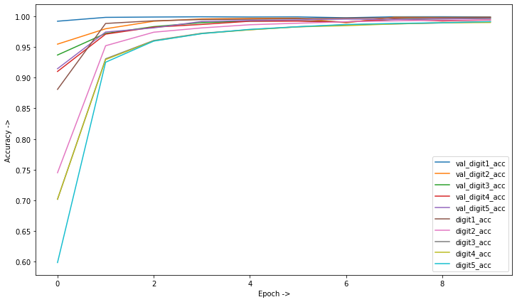
Figure 7.6: Training Accuracy for the model (7.5).

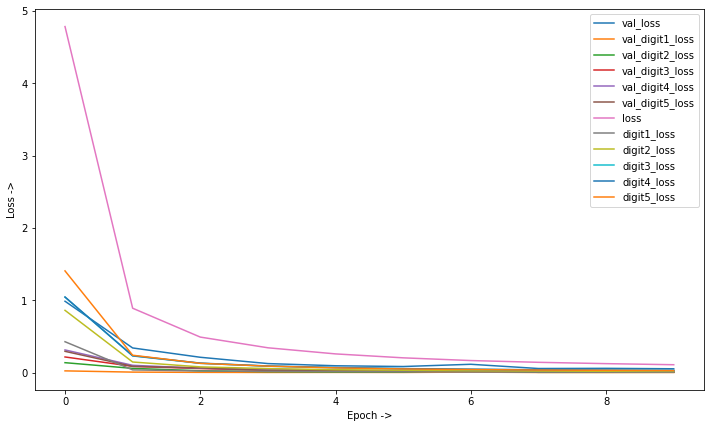
Figure 7.7: Training Loss for the model (7.5).

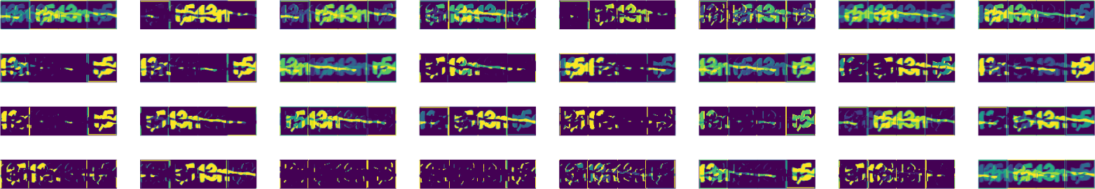
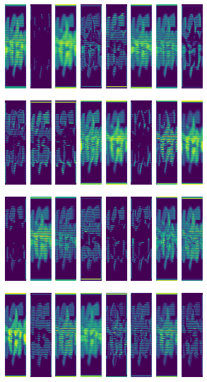
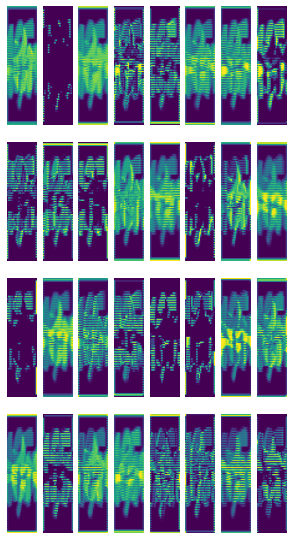
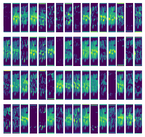
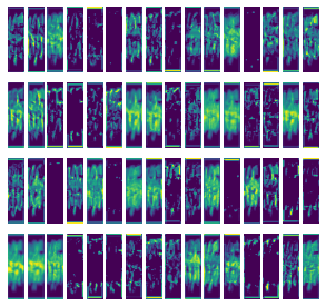
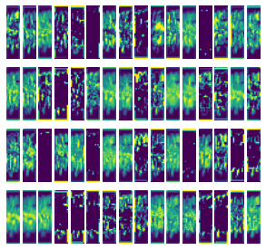
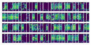
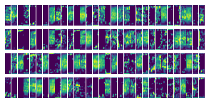
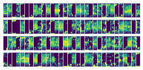
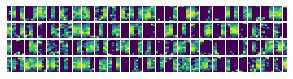
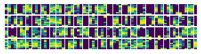
Figure 7.9: The visualizations of the features in a fully trained model (7.5) when passed a CAPTCHA containing the text r543n.

The summary of the model for 1L-labelled-CAPTCHAs dataset is shown in Figure 7.4. The summary for the epochs for the model is shown in Figure 7.1. It was trained on 30 epochs and each step of the epochs took about 71 seconds. This means that the total time taken for all of the computaion for 30 epochs is about 35.5 minutes. This is relatively slow as compared to the previous computation times as there are about 100000 images and the model has to go through each of the images for calculating the gradients. The images contained are of size 50x200 and is of binary images (i.e., intensity value of 0 and 255). This is a multi-label classification which has a total of 36 labels containing the lower-case ASCII letters (a-z) and the digits 0-9. Since, this has a total of 5 labels, there are 5 nodes that are coming out of the final layer, which helps in classifying the labels. The Keras visualization of the model is shown in Figure 7.5. The training accuracy of the model is shown in Figure 7.6 and the training loss is shown in Figure 7.7. The visualization of the intermediate layers of the learned model when a CAPTCHA containing the digit r543n is passed is shown in Figure 7.9. The CAPTCHA gave a total accuracy of 99.67% and it operates in human level. When passed through unseen data, we get predictions as shown in Figure 7.2. The trained model can be retrieved from this url (https://jimut123.github.io/blogs/CAPTCHA/models/images-1L-processed.h5). We see that all of the CAPTCHA is correctly classified incspite of the clutter in the background.

⬇

Epoch 10/10

72000/72000 [==============================] - 71s 991us/step - loss: 0.1094 - digit1_loss: 0.0055 - digit2_loss: 0.0171 - digit3_loss: 0.0281 - digit4_loss: 0.0317 - digit5_loss: 0.0270 - digit1_acc: 0.9982 - digit2_acc: 0.9942 - digit3_acc: 0.9911 - digit4_acc: 0.9900 - digit5_acc: 0.9914 - val_loss: 0.0532 - val_digit1_loss: 0.0023 - val_digit2_loss: 0.0049 - val_digit3_loss: 0.0095 - val_digit4_loss: 0.0212 - val_digit5_loss: 0.0154 - val_digit1_acc: 0.9991 - val_digit2_acc: 0.9984 - val_digit3_acc: 0.9968 - val_digit4_acc: 0.9940 - val_digit5_acc: 0.9967

Figure 7.1: Summary of the epochs after training the model (7.5).

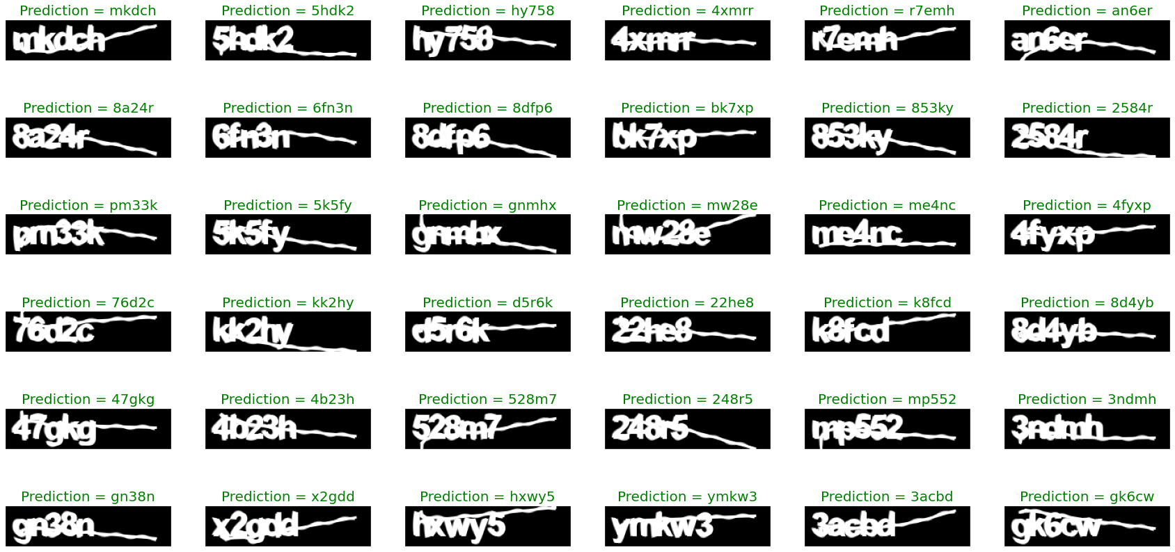
Figure 7.2: Predictions with the model (7.5).

Figure 7.3: The weights learned by the model (7.5) for layers 1 to 26.

⬇

__________________________________________________________________________________________________

Layer (type) Output Shape Param # Connected to

==================================================

input_1 (InputLayer) (None, 200, 50, 1) 0

__________________________________________________________________________________________________

conv2d_1 (Conv2D) (None, 200, 50, 32) 320 input_1[0][0]

__________________________________________________________________________________________________

conv2d_2 (Conv2D) (None, 198, 48, 32) 9248 conv2d_1[0][0]

__________________________________________________________________________________________________

batch_normalization_1 (BatchNor (None, 198, 48, 32) 128 conv2d_2[0][0]

__________________________________________________________________________________________________

max_pooling2d_1 (MaxPooling2D) (None, 99, 24, 32) 0 batch_normalization_1[0][0]

__________________________________________________________________________________________________

dropout_1 (Dropout) (None, 99, 24, 32) 0 max_pooling2d_1[0][0]

__________________________________________________________________________________________________

conv2d_3 (Conv2D) (None, 99, 24, 64) 18496 dropout_1[0][0]

__________________________________________________________________________________________________

conv2d_4 (Conv2D) (None, 97, 22, 64) 36928 conv2d_3[0][0]

__________________________________________________________________________________________________

batch_normalization_2 (BatchNor (None, 97, 22, 64) 256 conv2d_4[0][0]

__________________________________________________________________________________________________

max_pooling2d_2 (MaxPooling2D) (None, 48, 11, 64) 0 batch_normalization_2[0][0]

__________________________________________________________________________________________________

dropout_2 (Dropout) (None, 48, 11, 64) 0 max_pooling2d_2[0][0]

__________________________________________________________________________________________________

conv2d_5 (Conv2D) (None, 48, 11, 128) 73856 dropout_2[0][0]

__________________________________________________________________________________________________

conv2d_6 (Conv2D) (None, 46, 9, 128) 147584 conv2d_5[0][0]

__________________________________________________________________________________________________

batch_normalization_3 (BatchNor (None, 46, 9, 128) 512 conv2d_6[0][0]

__________________________________________________________________________________________________

max_pooling2d_3 (MaxPooling2D) (None, 23, 4, 128) 0 batch_normalization_3[0][0]

__________________________________________________________________________________________________

dropout_3 (Dropout) (None, 23, 4, 128) 0 max_pooling2d_3[0][0]

__________________________________________________________________________________________________

conv2d_7 (Conv2D) (None, 21, 2, 256) 295168 dropout_3[0][0]

__________________________________________________________________________________________________

batch_normalization_4 (BatchNor (None, 21, 2, 256) 1024 conv2d_7[0][0]

__________________________________________________________________________________________________

max_pooling2d_4 (MaxPooling2D) (None, 10, 1, 256) 0 batch_normalization_4[0][0]

__________________________________________________________________________________________________

flatten_1 (Flatten) (None, 2560) 0 max_pooling2d_4[0][0]

__________________________________________________________________________________________________

dropout_4 (Dropout) (None, 2560) 0 flatten_1[0][0]

__________________________________________________________________________________________________

digit1 (Dense) (None, 36) 92196 dropout_4[0][0]

__________________________________________________________________________________________________

digit2 (Dense) (None, 36) 92196 dropout_4[0][0]

__________________________________________________________________________________________________

digit3 (Dense) (None, 36) 92196 dropout_4[0][0]

__________________________________________________________________________________________________

digit4 (Dense) (None, 36) 92196 dropout_4[0][0]

__________________________________________________________________________________________________

digit5 (Dense) (None, 36) 92196 dropout_4[0][0]

==================================================

Total params: 1,044,500

Trainable params: 1,043,540

Non-trainable params: 960

__________________________________________________________________________________________________

Figure 7.4: Model (7.5) for identifying 1L-labelled-CAPTCHA dataset.

Figure 7.5: CIFAR 10 like model for identifying individual characters.

In Figure 7.8 we see the 3x3 kernels that are being learned by the layer 1 of the network for the Model 7.5. The visualization of the weights learned by the same model can be seen in Figure 7.3.

Figure 7.8: The 3x3 kernels (filter) learned by the model (7.5) for layer 1.

Chapter 8 Using faded CAPTCHA dataset (99.44 % accuracy)

8.1 AlexNet type model for faded CAPTCHA dataset

We have used an Alex-Net type model for the classification of the CAPTCHA. We haven’t performed any image operations and preserved the original size of the CAPTCHA data. The fundamental feature of the model which makes it different from others is it have a dropout layer before the last output in multilabel classification. This makes it robust to noise, since dropouts helps in training ensemble of Neural Networks. The summary of the model can be shown below.

⬇

_________________________________________________________________

Layer (type) Output Shape Param #

=================================================================

input_4 (InputLayer) [(None, 100, 120, 3)] 0

_________________________________________________________________

conv2d (Conv2D) (None, 98, 118, 32) 896

_________________________________________________________________

max_pooling2d (MaxPooling2D) (None, 49, 59, 32) 0

_________________________________________________________________

conv2d_1 (Conv2D) (None, 47, 57, 64) 18496

_________________________________________________________________

max_pooling2d_1 (MaxPooling2 (None, 23, 28, 64) 0

_________________________________________________________________

conv2d_2 (Conv2D) (None, 21, 26, 64) 36928

_________________________________________________________________

max_pooling2d_2 (MaxPooling2 (None, 10, 13, 64) 0

_________________________________________________________________

flatten (Flatten) (None, 8320) 0

_________________________________________________________________

dense (Dense) (None, 1024) 8520704

_________________________________________________________________

dropout (Dropout) (None, 1024) 0

_________________________________________________________________

dense_1 (Dense) (None, 40) 41000

_________________________________________________________________

reshape (Reshape) (None, 4, 10) 0

=================================================================

Total params: 8,618,024

Trainable params: 8,618,024

Non-trainable params: 0

_________________________________________________________________

The structure of the model when visualized in tensorboard can be found from figure 8.1. It took 10 epochs and a time of about 923 second per epochs. So, it basically took about 2.56 hours to finish the training. We can clearly see that it gets an accuracy of about 98.78% on the validation set and an accuracy of 99.44% on the test set, which is comparable to human level operators given the complexity and noise of this type of CAPTCHA. The loss and accuracy obtained from the training of the model is shown in Figure 8.3.

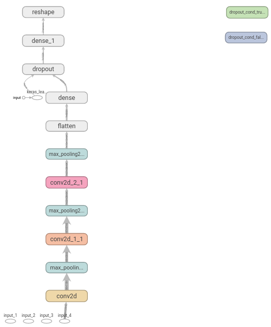
Figure 8.1: Alex-Net type model for multi-label classification.

⬇

Epoch 10/10

533/533 [==============================] - ETA: 0s - loss: 0.0386 - accuracy: 0.9878INFO:tensorflow:Assets written to: ./model_checkpoint/assets

533/533 [==============================] - 923s 2s/step - loss: 0.0386 - accuracy: 0.9878 - val_loss: 0.0186 - val_accuracy: 0.9944

Figure 8.2: epochs for faded CAPTCHA.

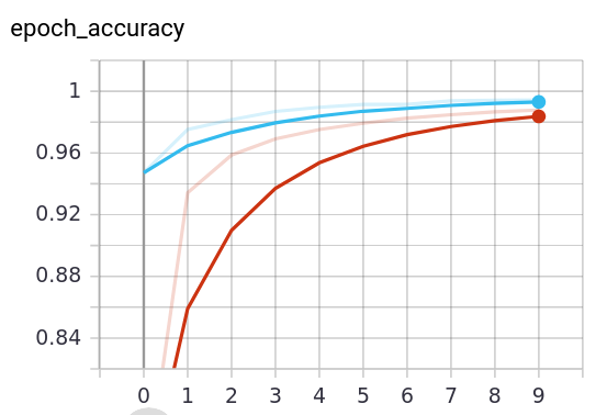
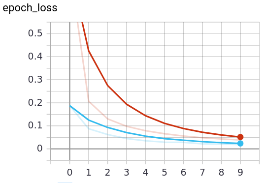
Figure 8.3: The accuracy and Loss obtained from the model when visualized via tensorboard.

When we test the model on unseen data, we get about 100% accuracy as shown in Figure 8.4. The model obtained can be found from here https://jimut123.github.io/blogs/CAPTCHA/models/faded_captcha.h5, which is about 98.7 MiB in size. From this we find that AlexNet have a capability of removing noise and generalizing well on unseen data.

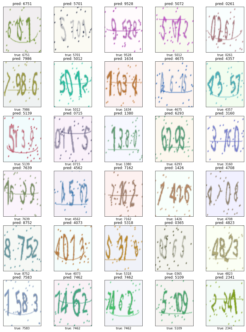
Figure 8.4: The prediction of the model with 100% accuracy on unseen data.

Chapter 9 Using Circle CAPTCHA dataset (99.99 % accuracy)

9.1 AlexNet type model for Circle CAPTCHA dataset

We have used a similar type of model, from 8.1, for preserving all the three channels of the CAPTCHA data. The summary of the model is shown below 9.1:

⬇

_________________________________________________________________

Layer (type) Output Shape Param #

==================================================

input_1 (InputLayer) [(None, 35, 120, 3)] 0

_________________________________________________________________

conv2d (Conv2D) (None, 33, 118, 32) 896

_________________________________________________________________

max_pooling2d (MaxPooling2D) (None, 16, 59, 32) 0

_________________________________________________________________

conv2d_1 (Conv2D) (None, 14, 57, 64) 18496

_________________________________________________________________

max_pooling2d_1 (MaxPooling2 (None, 7, 28, 64) 0

_________________________________________________________________

conv2d_2 (Conv2D) (None, 5, 26, 64) 36928

_________________________________________________________________

max_pooling2d_2 (MaxPooling2 (None, 2, 13, 64) 0

_________________________________________________________________

flatten (Flatten) (None, 1664) 0

_________________________________________________________________

dense (Dense) (None, 1024) 1704960

_________________________________________________________________

dropout (Dropout) (None, 1024) 0

_________________________________________________________________

dense_1 (Dense) (None, 216) 221400

_________________________________________________________________

reshape (Reshape) (None, 6, 36) 0

==================================================

Total params: 1,982,680

Trainable params: 1,982,680

Non-trainable params: 0

_________________________________________________________________

Figure 9.1: Summary of the model for 13.3.

The Model was trained for 10 epochs and it gave a validation accuracy of 99.99% and 99.98% on the test set. This is pretty good result since the model kind of learns from the little circular marks on the dataset that they are just noise. The model took about 650 second per epochs and a total of 1.80 hours for finishing the training for 10 epochs. The model can be found from this link (https://jimut123.github.io/blogs/CAPTCHA/models/circle_captcha_10e.h5). The size of the model is about 22.7 MiB. The structure of the model is shown in Figure 9.3, the visualization of the accuracy of the model is shown in Figure 9.4, and the loss for the same model is shown in Figure 9.5. The prediction of the model is shown in Figure 9.6, on unseen data, and it accurately classifies all the labels of the CAPTCHA.

⬇

Epoch 10/10

392/392 [==============================] - ETA: 0s - loss: 0.0147 - accuracy: 0.9951INFO:tensorflow:Assets written to: ./model_checkpoint/assets

392/392 [==============================] - 650s 2s/step - loss: 0.0147 - accuracy: 0.9951 - val_loss: 6.1774e-04 - val_accuracy: 0.9999

Figure 9.2: epochs for circle CAPTCHA.

Figure 9.3: Keras model structure for Circle CAPTCHA.

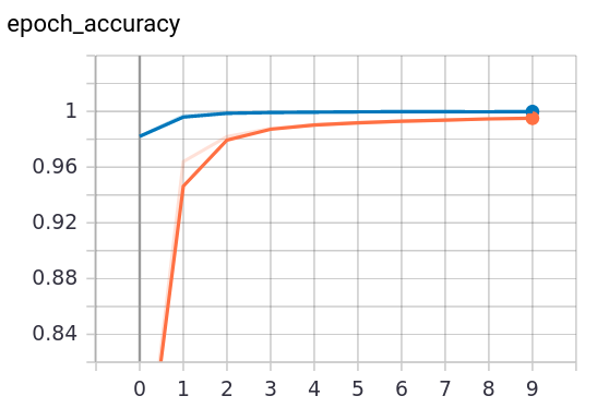
Figure 9.4: Accuracy of the model (9.3).

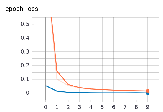
Figure 9.5: Loss of the model (9.3).

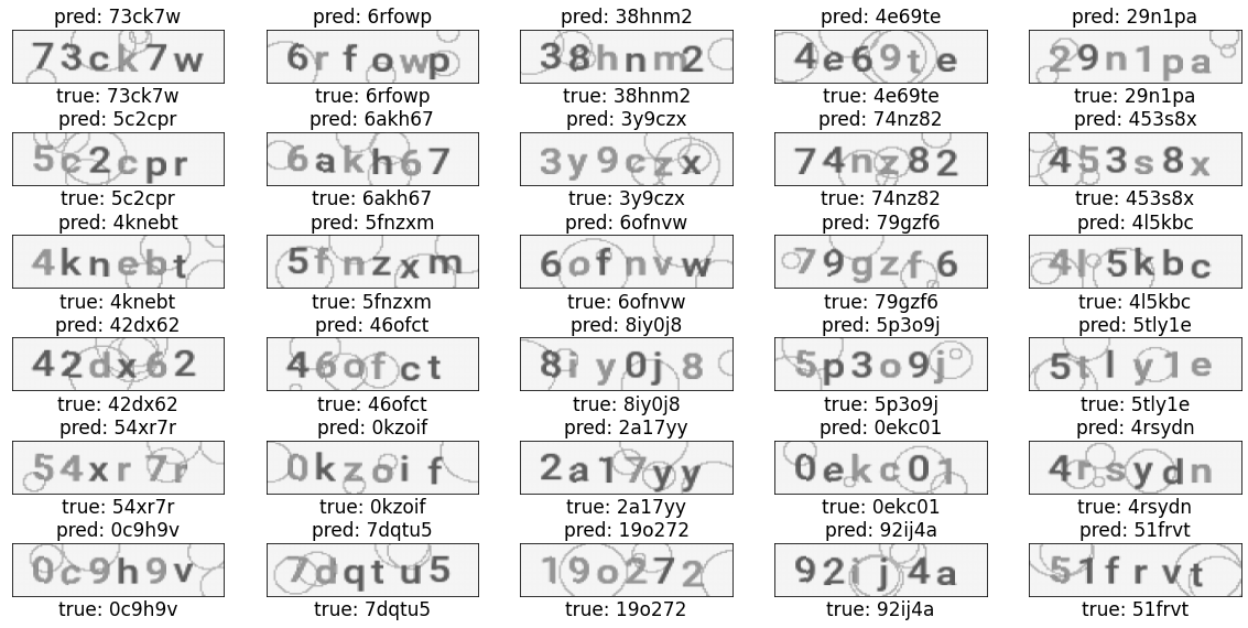
Figure 9.6: Predictions of the model (9.3).

Chapter 10 Using Sphinx CAPTCHA dataset (99.62 % accuracy)

10.1 AlexNet type model for faded CAPTCHA dataset

We have used a similar type of model, from 8.1, for preserving all the three channels of the CAPTCHA data. The summary of the model is shown below 10.1:

⬇

_________________________________________________________________

Layer (type) Output Shape Param #

==================================================

input_1 (InputLayer) [(None, 40, 150, 3)] 0

_________________________________________________________________

conv2d (Conv2D) (None, 38, 148, 32) 896

_________________________________________________________________

max_pooling2d (MaxPooling2D) (None, 19, 74, 32) 0

_________________________________________________________________

conv2d_1 (Conv2D) (None, 17, 72, 64) 18496

_________________________________________________________________

max_pooling2d_1 (MaxPooling2 (None, 8, 36, 64) 0

_________________________________________________________________

conv2d_2 (Conv2D) (None, 6, 34, 64) 36928

_________________________________________________________________

max_pooling2d_2 (MaxPooling2 (None, 3, 17, 64) 0

_________________________________________________________________

flatten (Flatten) (None, 3264) 0

_________________________________________________________________

dense (Dense) (None, 1024) 3343360

_________________________________________________________________

dropout (Dropout) (None, 1024) 0

_________________________________________________________________

dense_1 (Dense) (None, 76) 77900

_________________________________________________________________

reshape (Reshape) (None, 4, 19) 0

==================================================

Total params: 3,477,580

Trainable params: 3,477,580

Non-trainable params: 0

_________________________________________________________________

Figure 10.1: Summary of the model for 13.3.

The model is trained for about 15 epochs. Each epoch took about 1293 second, which means it took about 5.3875 hours to train the whole model. The summary of the epochs is shown in 10.2. The summary of the 15th epochs is about 99.62 % accuracy on the validation set and test set, which means it is able to capture the characters from the noise very well. It is able to generalize the data pretty good.

⬇

Epoch 15/15

446/446 [==============================] - ETA: 0s - loss: 0.0503 - accuracy: 0.9833INFO:tensorflow:Assets written to: ./model_checkpoint/assets

446/446 [==============================] - 1293s 3s/step - loss: 0.0503 - accuracy: 0.9833 - val_loss: 0.0125 - val_accuracy: 0.9962

Figure 10.2: epochs for sphinx CAPTCHA.

The training accuracy and loss can be shown in Figure 10.4 and 10.5 respectively. The prediction of the model on unseen data can be seen in Figure 10.6. This is like human level accuracy and this CAPTCHA is widely used over the internet. So, AlexNet type model can capture the necessary information very well and differentiate from noise very well. The whole CAPTCHA data is about 12.7 GB and the model is of size 39.9 MB. The model can be obtained from this link (https://jimut123.github.io/blogs/CAPTCHA/models/sphinx_full_34_15e_9962.h5).

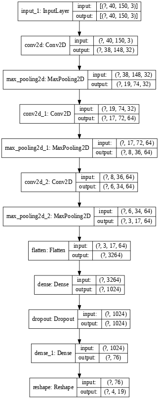
Figure 10.3: Tensorboard Visualization of the structure of the model (6.8).

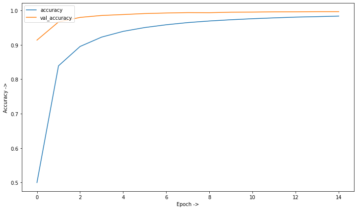
Figure 10.4: Accuracy of the model (10.3).

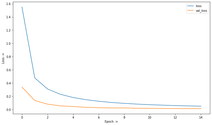
Figure 10.5: Loss of the model (10.3).

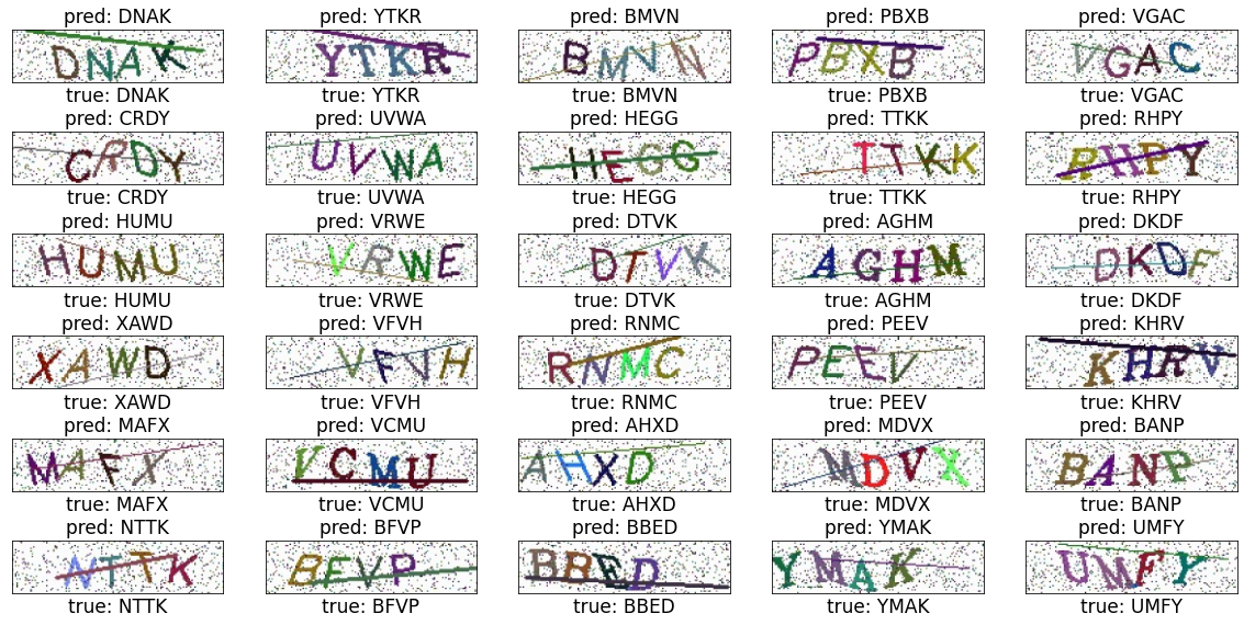
Figure 10.6: Predictions of the model (10.3).

Chapter 11 Using fish eye dataset (99.46 % accuracy)

11.1 Using AlexNet type Model

Since there is a lot of clutter in the CAPTCHA dataset, we will use this AlexNet type model. The summary of the model is shown in Figure 11.1. This is similar to the type of model shown in Figure 8.1, except the fact that there are 5 outgoing labels from the final layer of the model. The dataset was trained using this model, and the accuracy obtained can be shown in Figure 11.2. It took about 3902 second per epochs and there was a total of 5 epochs. The total training time was about 10.83 hours, which is too much. The plot of the model can be seen in Figure 11.3. The accuracy obtained on training’s validation set was about 97.49 % and the same for test dataset was 99.46 % which was pretty great given that the model converges in only 5 epochs. Since the data size was too large, so we did a batch-based training where the training batch size was about 2048 and validation batch size was 512. The trained model can be obtained from the following link (https://jimut123.github.io/blogs/CAPTCHA/models/fish_eye.h5).

The accuracy and the loss obtained by the model can be shown in Figure 11.4 and Figure 11.5 respectively. The predictions of the model on fully unseen data is shown in Figure 11.6, which shows that it predicts almost all of the CAPTCHA labels correctly and is able to generalize well on completely unseen data. The only wrong classifications it wrongly classified was 2rrx4 as 2rrr4, frb6g as frh6g, and faff8 as faff5 which is even difficult for humans to classify correctly since the letters were cluttered in occlusion.

⬇

_________________________________________________________________

_________________________________________________________________

Layer (type) Output Shape Param #

==================================================

input_1 (InputLayer) [(None, 50, 200, 3)] 0

_________________________________________________________________

conv2d (Conv2D) (None, 48, 198, 32) 896

_________________________________________________________________

max_pooling2d (MaxPooling2D) (None, 24, 99, 32) 0

_________________________________________________________________

conv2d_1 (Conv2D) (None, 22, 97, 64) 18496

_________________________________________________________________

max_pooling2d_1 (MaxPooling2 (None, 11, 48, 64) 0

_________________________________________________________________

conv2d_2 (Conv2D) (None, 9, 46, 64) 36928

_________________________________________________________________

max_pooling2d_2 (MaxPooling2 (None, 4, 23, 64) 0

_________________________________________________________________

flatten (Flatten) (None, 5888) 0

_________________________________________________________________

dense (Dense) (None, 1024) 6030336

_________________________________________________________________

dropout (Dropout) (None, 1024) 0

_________________________________________________________________

dense_1 (Dense) (None, 115) 117875

_________________________________________________________________

reshape (Reshape) (None, 5, 23) 0

==================================================

Total params: 6,204,531

Trainable params: 6,204,531

Non-trainable params: 0

_________________________________________________________________

Figure 11.1: Summary of the AlexNet type model for classifying the labels of fish eye CAPTCHA dataset.

⬇

881/881 [==============================] - 3902s 4s/step - loss: 0.0725 - accuracy: 0.9749 - val_loss: 0.0167 - val_accuracy: 0.9946

Figure 11.2: Summary of epochs for the model (6.8).

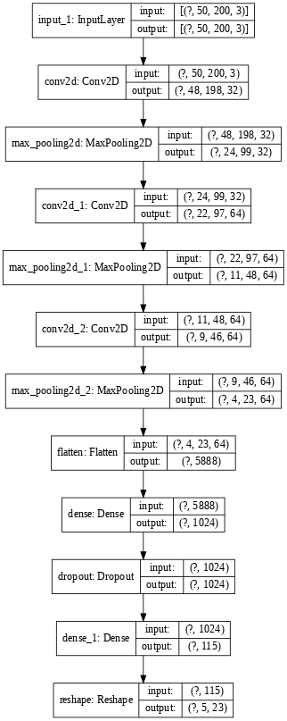
Figure 11.3: Tensorboard Visualization of the structure of the model (6.8).

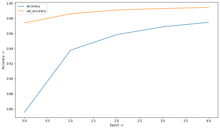
Figure 11.4: Accuracy of the model (11.3).

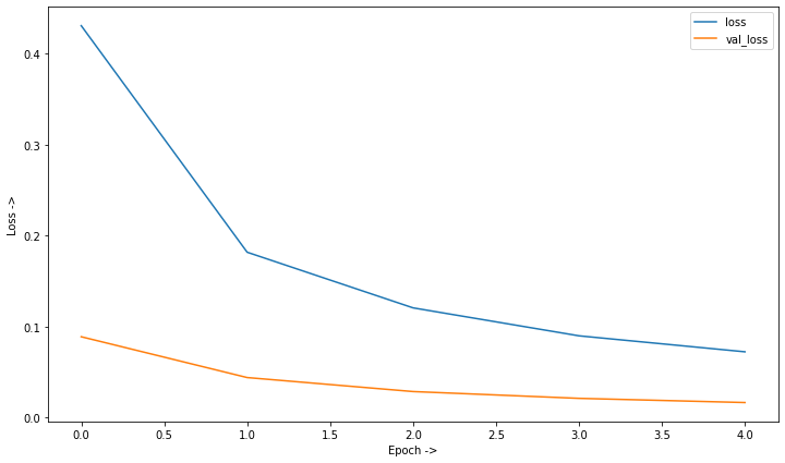
Figure 11.5: Loss of the model (11.3).

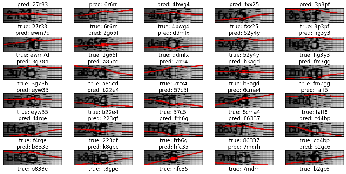
Figure 11.6: Predictions of the model (11.3).

Chapter 12 Using Mini CAPTCHA dataset (97.25 % accuracy)

12.1 AlexNet type model for Mini CAPTCHA dataset

We have used a similar type of model, from 8.1, for preserving all the three channels of the CAPTCHA data. The summary of the model is shown below 12.1:

⬇

_________________________________________________________________

Layer (type) Output Shape Param #

==================================================

input_1 (InputLayer) [(None, 100, 264, 3)] 0

_________________________________________________________________

conv2d (Conv2D) (None, 98, 262, 32) 896

_________________________________________________________________

max_pooling2d (MaxPooling2D) (None, 49, 131, 32) 0

_________________________________________________________________

conv2d_1 (Conv2D) (None, 47, 129, 64) 18496

_________________________________________________________________

max_pooling2d_1 (MaxPooling2 (None, 23, 64, 64) 0

_________________________________________________________________

conv2d_2 (Conv2D) (None, 21, 62, 64) 36928

_________________________________________________________________

max_pooling2d_2 (MaxPooling2 (None, 10, 31, 64) 0

_________________________________________________________________

flatten (Flatten) (None, 19840) 0

_________________________________________________________________

dense (Dense) (None, 1024) 20317184

_________________________________________________________________

dropout (Dropout) (None, 1024) 0

_________________________________________________________________

dense_1 (Dense) (None, 248) 254200

_________________________________________________________________

reshape (Reshape) (None, 4, 62) 0

==================================================

Total params: 20,627,704

Trainable params: 20,627,704

Non-trainable params: 0

_________________________________________________________________

Figure 12.1: Summary of the model for 13.3.

The Model was trained for 10 epochs and it gave a validation accuracy of 97.25% and 97.09% on the test set. This is pretty good result since the model learns a whole lot of class to classify and generalizes well on unseen data. The model took about 2070 second per epochs and a total of 5.75 hours for finishing the training for 10 epochs. The model can be found from this link (https://drive.google.com/open?id=1w5BhaeSvc1LYQfUuvwBApeNbcx0vkOUP). The size of the model is about 236 MiB.

The structure of the model is shown in Figure 12.3, the visualization of the accuracy of the model is shown in Figure 12.4, and the loss for the same model is shown in Figure 12.5. The prediction of the model is shown in Figure 12.6, on unseen data, and it accurately classifies all the labels of the CAPTCHA.

⬇

Epoch 10/10

1762/1762 [==============================] - ETA: 0s - loss: 0.3160 - accuracy: 0.8926INFO:tensorflow:Assets written to: ./model_checkpoint/assets

1762/1762 [==============================] - 2070s 1s/step - loss: 0.3160 - accuracy: 0.8926 - val_loss: 0.0920 - val_accuracy: 0.9725

Figure 12.2: epochs for mini CAPTCHA.

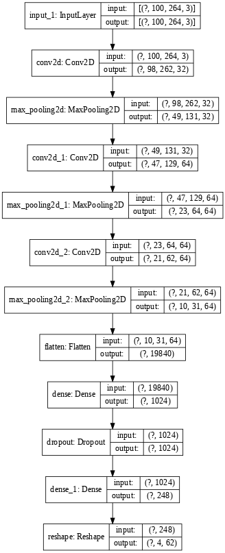
Figure 12.3: Keras model structure for Circle CAPTCHA.

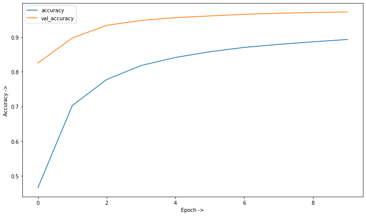
Figure 12.4: Accuracy of the model (12.3).

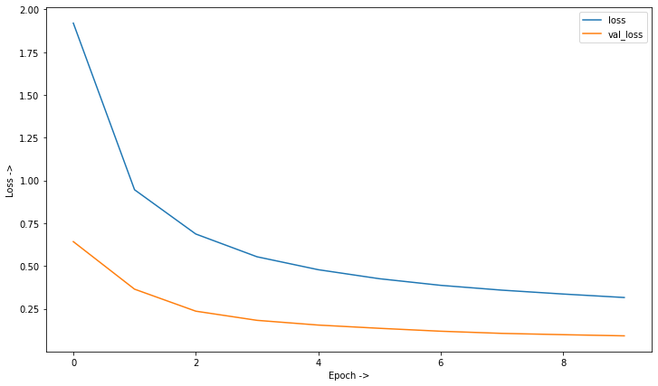
Figure 12.5: Loss of the model (12.3).

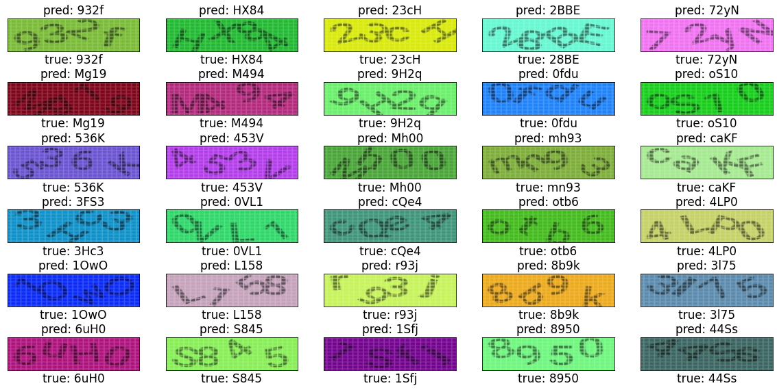
Figure 12.6: Predictions of the model (12.3).

Chapter 13 Using Multicolor CAPTCHA dataset (95.69 % accuracy)

13.1 Alex Net type model for Multicolor CAPTCHA dataset

The initial version of the dataset contained a black background which was significantly reducing the information, by cluttering the convnet as shown in Figure 2.34. We needed to crop the image before feeding into the convolutional neural network. We have trained the dataset using the model similar to Model 8.1. The details of the dataset can be found on the appendix section and we have used only 50% of the multicolor dataset for this purpose.

The summary of the model is shown below 13.1, and the summary of the epochs is shown 13.2. The model is stopped early because of getting a low loss, and minimizing the loss as much as possible. It could great even better result but this is pretty doable for a hard CAPTCHA like this. We claim that the loss could even go down, resulting in increase of accuracy if we trained it for a little more time. The model for the same is shown in figure 13.3.

⬇

_________________________________________________________________

Layer (type) Output Shape Param #

==================================================

input_1 (InputLayer) [(None, 150, 640, 4)] 0

_________________________________________________________________

conv2d (Conv2D) (None, 148, 638, 32) 1184

_________________________________________________________________

max_pooling2d (MaxPooling2D) (None, 74, 319, 32) 0

_________________________________________________________________

conv2d_1 (Conv2D) (None, 72, 317, 64) 18496

_________________________________________________________________

max_pooling2d_1 (MaxPooling2 (None, 36, 158, 64) 0

_________________________________________________________________

conv2d_2 (Conv2D) (None, 34, 156, 64) 36928

_________________________________________________________________

max_pooling2d_2 (MaxPooling2 (None, 17, 78, 64) 0

_________________________________________________________________

flatten (Flatten) (None, 84864) 0

_________________________________________________________________

dense (Dense) (None, 1024) 86901760

_________________________________________________________________

dropout (Dropout) (None, 1024) 0

_________________________________________________________________

dense_1 (Dense) (None, 40) 41000

_________________________________________________________________

reshape (Reshape) (None, 4, 10) 0

==================================================

Total params: 86,999,368

Trainable params: 86,999,368

Non-trainable params: 0

_________________________________________________________________

Figure 13.1: Summary of the model for 13.3.

⬇

Epoch 9/20

3525/3525 [==============================] - ETA: 0s - loss: 0.2153 - accuracy: 0.9245INFO:tensorflow:Assets written to: ./model_checkpoint/assets

3525/3525 [==============================] - 3464s 983ms/step - loss: 0.2153 - accuracy: 0.9245 - val_loss: 0.1315 - val_accuracy: 0.9569

Figure 13.2: The summary of 9 epochs for the model 13.3.

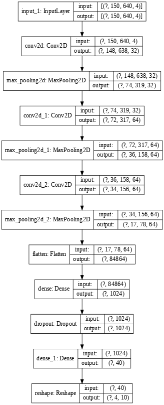
Figure 13.3: Our model for predicting the labels of the multicolor CAPTCHA dataset.

The loss and accuracy plots for the mentioned model is shown in Figure 13.5 and Figure 13.4. The model took about 3482 seconds for each of the epochs which is about 8.705 hours for the complete training for 9 epochs. The model generated (in .h5 format) can be found on this drive link https://drive.google.com/open?id=1-2DW3CBkddRoUsBbaukf7OxR1MZpwVrn. The size of the model is 996 MB, since is due to the fact that the model captures many details of the huge dataset. We see that the model trained generalizes well on the unseen data as shown in Figure 13.6. The accuracy of the model obtained is 95.69% which is pretty great for an AlexNet type model. This is one of the hardest open source CAPTCHAs even for the humans because these contains a variety of colors, and those who suffer from night blindness, will find it difficult to predict the letters of this CAPTCHA accurately.

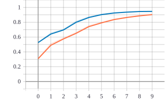
Figure 13.4: Plot for the training accuracy of our model.

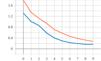
Figure 13.5: Plot for the training loss of our model.

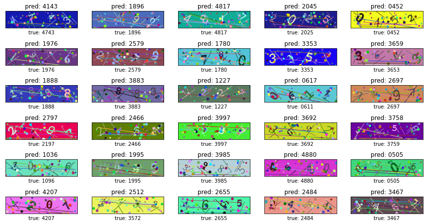
Figure 13.6: Prediction of the new model (13.3) on unseen data.

Chapter 14 Determining complexity of CAPTCHAs through Railway-CAPTCHA

Our main objective in this section is to see how complexity of CAPTCHA increases with the length of the CAPTCHA for multilabel classification. Here we use a similar model to test all the CAPTCHAs with varying length, ranging from 3 to 7, with 100K sample of data (both test, validation, and training data included). We conjecture that the length of the CAPTCHA increases the complexity of CAPTCHA when it is hard to segment each letter and the CAPTCHA is noisy. A human can read a paragraph of simple letters with some noise with no hindrance, but it takes a lot of time for computers to do the same task. This is the reason why there is no perfect OCR for storing the documents of Guttenberg project to text digitally, which is still a problem for data retrieval. Whereas humans have seen too much of textual data in their entire life, so they can understand quickly what a paper-document is saying in different lighting conditions. This is the reason why there are still many sites which still rely on long length text CAPTCHAs to save their resources.

14.1 Railway-CAPTCHA with 3 Letters

⬇

__________________________________________________________________________________________________

Layer (type) Output Shape Param # Connected to

==================================================

input_1 (InputLayer) (None, 200, 60, 1) 0

__________________________________________________________________________________________________

conv2d_1 (Conv2D) (None, 200, 60, 32) 320 input_1[0][0]

__________________________________________________________________________________________________

conv2d_2 (Conv2D) (None, 198, 58, 32) 9248 conv2d_1[0][0]

__________________________________________________________________________________________________

batch_normalization_1 (BatchNor (None, 198, 58, 32) 128 conv2d_2[0][0]

__________________________________________________________________________________________________

max_pooling2d_1 (MaxPooling2D) (None, 99, 29, 32) 0 batch_normalization_1[0][0]

__________________________________________________________________________________________________

dropout_1 (Dropout) (None, 99, 29, 32) 0 max_pooling2d_1[0][0]

__________________________________________________________________________________________________

conv2d_3 (Conv2D) (None, 99, 29, 64) 18496 dropout_1[0][0]

__________________________________________________________________________________________________

conv2d_4 (Conv2D) (None, 97, 27, 64) 36928 conv2d_3[0][0]

__________________________________________________________________________________________________

batch_normalization_2 (BatchNor (None, 97, 27, 64) 256 conv2d_4[0][0]

__________________________________________________________________________________________________

max_pooling2d_2 (MaxPooling2D) (None, 48, 13, 64) 0 batch_normalization_2[0][0]

__________________________________________________________________________________________________

dropout_2 (Dropout) (None, 48, 13, 64) 0 max_pooling2d_2[0][0]

__________________________________________________________________________________________________

conv2d_5 (Conv2D) (None, 48, 13, 128) 73856 dropout_2[0][0]

__________________________________________________________________________________________________

conv2d_6 (Conv2D) (None, 46, 11, 128) 147584 conv2d_5[0][0]

__________________________________________________________________________________________________

batch_normalization_3 (BatchNor (None, 46, 11, 128) 512 conv2d_6[0][0]

__________________________________________________________________________________________________

max_pooling2d_3 (MaxPooling2D) (None, 23, 5, 128) 0 batch_normalization_3[0][0]

__________________________________________________________________________________________________

dropout_3 (Dropout) (None, 23, 5, 128) 0 max_pooling2d_3[0][0]

__________________________________________________________________________________________________

conv2d_7 (Conv2D) (None, 21, 3, 256) 295168 dropout_3[0][0]

__________________________________________________________________________________________________

batch_normalization_4 (BatchNor (None, 21, 3, 256) 1024 conv2d_7[0][0]

__________________________________________________________________________________________________

max_pooling2d_4 (MaxPooling2D) (None, 10, 1, 256) 0 batch_normalization_4[0][0]

__________________________________________________________________________________________________

flatten_1 (Flatten) (None, 2560) 0 max_pooling2d_4[0][0]

__________________________________________________________________________________________________

dropout_4 (Dropout) (None, 2560) 0 flatten_1[0][0]

__________________________________________________________________________________________________

digit1 (Dense) (None, 36) 87074 dropout_4[0][0]

__________________________________________________________________________________________________

digit2 (Dense) (None, 36) 87074 dropout_4[0][0]

__________________________________________________________________________________________________

digit3 (Dense) (None, 36) 87074 dropout_4[0][0]

==================================================

Total params: 844,742

Trainable params: 843,782

Non-trainable params: 960

__________________________________________________________________________________________________

Figure 14.1: Summary of the vanilla model (14.3) for railway 3 letter CAPTCHA dataset.

⬇

Epoch 30/30

72000/72000 [==============================] - 81s 1ms/step - loss: 2.3520 - digit1_loss: 0.7551 - digit2_loss: 0.8290 - digit3_loss: 0.7678 - digit1_acc: 0.7729 - digit2_acc: 0.7508 - digit3_acc: 0.7699 - val_loss: 2.3121 - val_digit1_loss: 0.7538 - val_digit2_loss: 0.7967 - val_digit3_loss: 0.7616 - val_digit1_acc: 0.8068 - val_digit2_acc: 0.7862 - val_digit3_acc: 0.8023

Figure 14.2: Summary of the epochs for the vanilla model (14.3) for railway 3 letter CAPTCHA dataset.

We started our experiment with the open source synthetic CAPTCHA data generator by this CAPTCHA of 3 letters. We used our previous models and tried to improve on the existing models. The summary of the model is shown in Figure 14.1. This is generated by the Keras’s $model.summary()$ method. The epochs of the model is shown in Figure 14.2. It took about 81 second per epochs and there was a total of 30 epochs. The total time of training for the model was about 40.5 minutes, which is okay, since there is a total of 100K images of 3 letter CAPTCHA. This is again a multi-label classification which classified about 36 labels, i.e., all the 26 capital letters from A to Z and all the digits 0 to 9. The images are of 60x200 size and they are all preprocessed before passing to the naive version of the model. The preprocessing of the image is shown in Figure 14.6. The original images are of 3 channels, i.e., red, green and blue channels. It is then converted to grayscale and then applied binary inverse thresholding to make the image in binary format (i.e., intensity values of 255 and 0 only). Here all those pixels intensity which is less than 127 is set to 255 and all the pixels which are greater than 127 is set to 0. Then the resultant image formed, has some noise in them. This is because of the nature of the image to make the computer confused and make humans easy to decipher what code is written in them. To remove the noise, we perform erosion to make them thinner and then dilation to make them thicker. Then it is passed to the model for getting better results. The graph layout of the model when visualized with Keras is shown in Figure 14.3. The training accuracy obtained for the model is shown in Figure 14.4 and the loss is shown in Figure 14.5. The accuracy obtained from this model is about 80% which is still low compared to the human level operator and other models that we built. The prediction of the model trained on some random unseen images is shown in Figure 14.8. The trained model can be retrieved from this url (https://jimut123.github.io/blogs/CAPTCHA/models/railway_captcha_3.h5). We see that 9 out of 36 images are incorrect, which is still bad and we have a lot to improve on this model. The CAPTCHA image for this kind is a little bit trickier to train. There is various clutter and occlusion of the resultant binary image which makes the model confuse which label to classify and predict. We need to improve on the preprocessing step to make clear images which can help the model to learn better CAPTCHA and predict them correctly. The visualization of the layers of the model when passed through an image as shown in Figure 14.7 is shown in Figure 14.3.

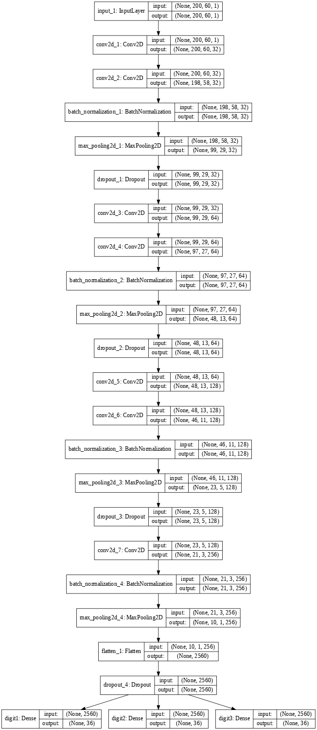
Figure 14.3: The vanilla model for railway 3 letter CAPTCHA dataset.

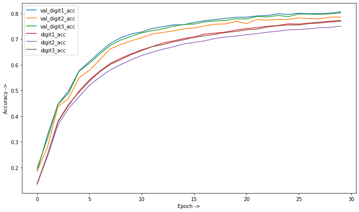
Figure 14.4: Training Accuracy for the vanilla model (14.3).

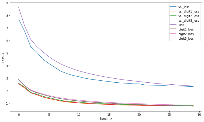
Figure 14.5: Training Loss for the vanilla model (14.3).

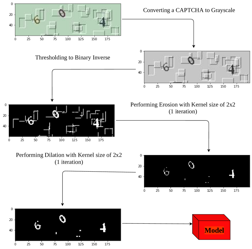
Figure 14.6: The preprocessing done to improve accuracy before feeding it to the model (14.3).

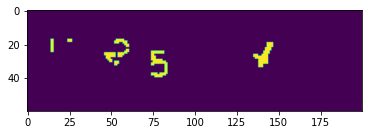
Figure 14.7: A CAPTCHA of 254 was given to the layer of the model (14.3) for visualizations.

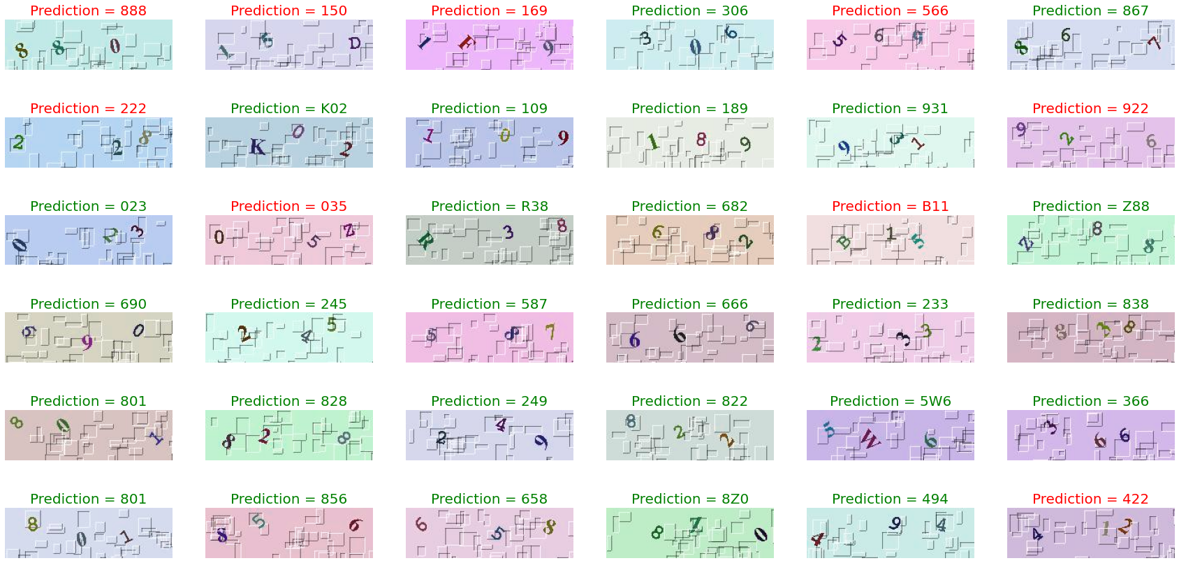
Figure 14.8: Predictions of the model (14.3).

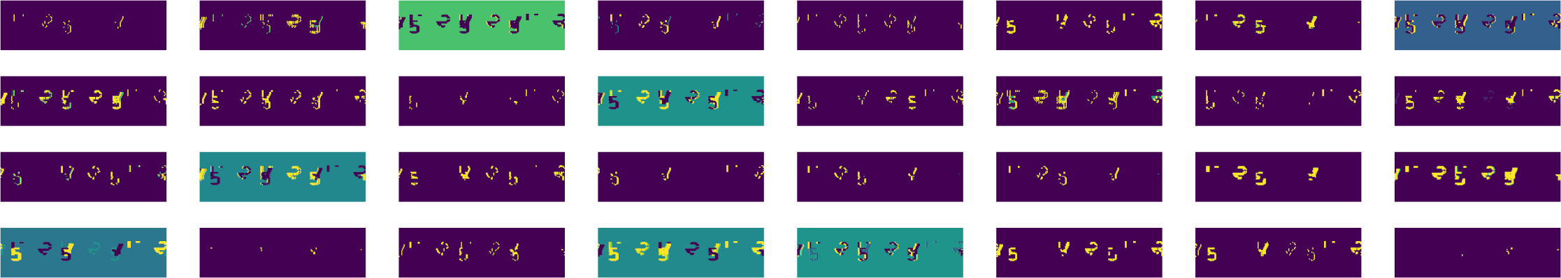
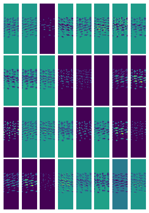
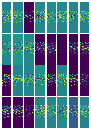
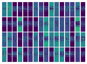
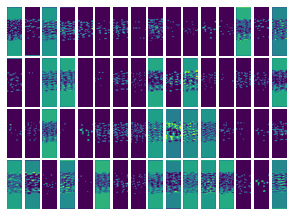
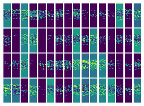
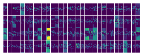
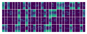
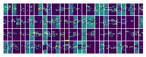
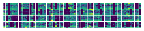
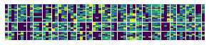
Figure 14.9: The visualizations of the features in a fully trained model 14.3 when passed a CAPTCHA containing the characters 254.

14.2 Railway-CAPTCHA with 4 Letters

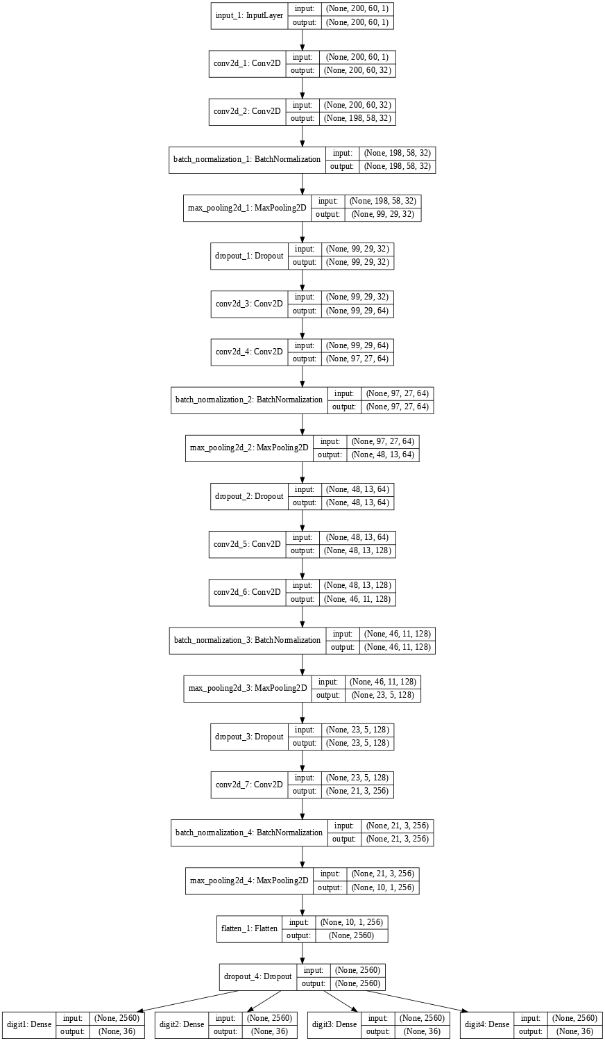
Figure 14.12: Our vanilla model for cracking 4-letter railway CAPTCHA.

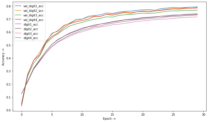
Figure 14.13: Training Accuracy for the model (14.12).

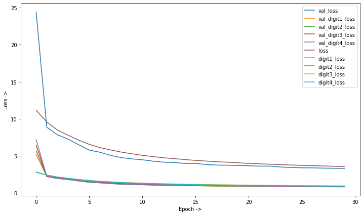
Figure 14.14: Training Loss for the model (14.12).

We then checked how the same model performs with CAPTCHAs generated from the same dataset but this time with 4-character length labels. Here, the size and dimensions of the image are same as the previous one, the pre-processing done on the image is same too. We just changed some of the output nodes of the model and checked how this performed. The summary of the model is shown in Figure 14.10. The summary of the epochs is shown in Figure 14.11. It takes about 87 seconds to complete one epoch and a total of 43.5 minutes to finish the training. The graph layout of the model is shown in Figure 14.12. The accuracy obtained is about 79% and the plot is shown in Figure 14.13. The trained model can be retrieved from this url (https://jimut123.github.io/blogs/CAPTCHA/models/railway_captcha_4_imop.h5). The plot for the loss for the same model is shown in Figure 14.14. When the model is tested on real world unseen data, we get the prediction of 14.15, which shows that the performance is not so well on real world data. The model predicts 18 images wrongly out of 36 images which is way more less than human level operator.

⬇

__________________________________________________________________________________________________

Layer (type) Output Shape Param # Connected to

==================================================

input_1 (InputLayer) (None, 200, 60, 1) 0

__________________________________________________________________________________________________

conv2d_1 (Conv2D) (None, 200, 60, 32) 320 input_1[0][0]

__________________________________________________________________________________________________

conv2d_2 (Conv2D) (None, 198, 58, 32) 9248 conv2d_1[0][0]

__________________________________________________________________________________________________

batch_normalization_1 (BatchNor (None, 198, 58, 32) 128 conv2d_2[0][0]

__________________________________________________________________________________________________

max_pooling2d_1 (MaxPooling2D) (None, 99, 29, 32) 0 batch_normalization_1[0][0]

__________________________________________________________________________________________________

dropout_1 (Dropout) (None, 99, 29, 32) 0 max_pooling2d_1[0][0]

__________________________________________________________________________________________________

conv2d_3 (Conv2D) (None, 99, 29, 64) 18496 dropout_1[0][0]

__________________________________________________________________________________________________

conv2d_4 (Conv2D) (None, 97, 27, 64) 36928 conv2d_3[0][0]

__________________________________________________________________________________________________

batch_normalization_2 (BatchNor (None, 97, 27, 64) 256 conv2d_4[0][0]

__________________________________________________________________________________________________

max_pooling2d_2 (MaxPooling2D) (None, 48, 13, 64) 0 batch_normalization_2[0][0]

__________________________________________________________________________________________________

dropout_2 (Dropout) (None, 48, 13, 64) 0 max_pooling2d_2[0][0]

__________________________________________________________________________________________________

conv2d_5 (Conv2D) (None, 48, 13, 128) 73856 dropout_2[0][0]

__________________________________________________________________________________________________

conv2d_6 (Conv2D) (None, 46, 11, 128) 147584 conv2d_5[0][0]

__________________________________________________________________________________________________

batch_normalization_3 (BatchNor (None, 46, 11, 128) 512 conv2d_6[0][0]

__________________________________________________________________________________________________

max_pooling2d_3 (MaxPooling2D) (None, 23, 5, 128) 0 batch_normalization_3[0][0]

__________________________________________________________________________________________________

dropout_3 (Dropout) (None, 23, 5, 128) 0 max_pooling2d_3[0][0]

__________________________________________________________________________________________________

conv2d_7 (Conv2D) (None, 21, 3, 256) 295168 dropout_3[0][0]

__________________________________________________________________________________________________

batch_normalization_4 (BatchNor (None, 21, 3, 256) 1024 conv2d_7[0][0]

__________________________________________________________________________________________________

max_pooling2d_4 (MaxPooling2D) (None, 10, 1, 256) 0 batch_normalization_4[0][0]

__________________________________________________________________________________________________

flatten_1 (Flatten) (None, 2560) 0 max_pooling2d_4[0][0]

__________________________________________________________________________________________________

dropout_4 (Dropout) (None, 2560) 0 flatten_1[0][0]

__________________________________________________________________________________________________

digit1 (Dense) (None, 36) 87074 dropout_4[0][0]

__________________________________________________________________________________________________

digit2 (Dense) (None, 36) 87074 dropout_4[0][0]

__________________________________________________________________________________________________

digit3 (Dense) (None, 36) 87074 dropout_4[0][0]

__________________________________________________________________________________________________

digit4 (Dense) (None, 36) 87074 dropout_4[0][0]

==================================================

Total params: 931,816

Trainable params: 930,856

Non-trainable params: 960

__________________________________________________________________________________________________

Figure 14.10: Model 14.12 Summary for cracking 4-letter railway CAPTCHA.

⬇

Epoch 30/30

72000/72000 [==============================] - 87s 1ms/step - loss: 3.5429 - digit1_loss: 0.8553 - digit2_loss: 0.8677 - digit3_loss: 0.9308 - digit4_loss: 0.8891 - digit1_acc: 0.7397 - digit2_acc: 0.7362 - digit3_acc: 0.7162 - digit4_acc: 0.7309 - val_loss: 3.2911 - val_digit1_loss: 0.7909 - val_digit2_loss: 0.8026 - val_digit3_loss: 0.8854 - val_digit4_loss: 0.8121 - val_digit1_acc: 0.7937 - val_digit2_acc: 0.7886 - val_digit3_acc: 0.7672 - val_digit4_acc: 0.7839

Figure 14.11: Model 14.12 Summary.

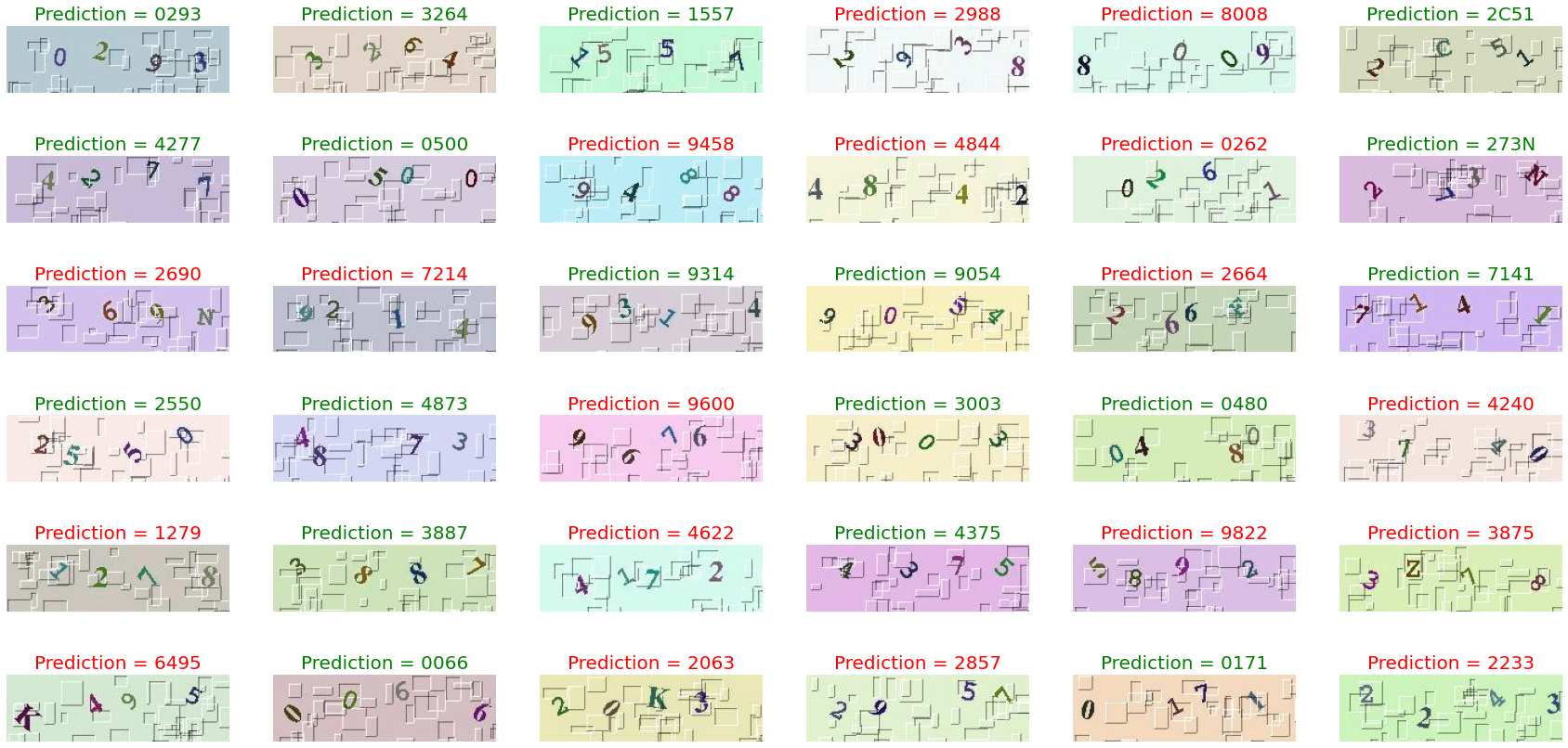
Figure 14.15: Predictions of the model (14.12).

14.3 Railway-CAPTCHA with 5 Letters

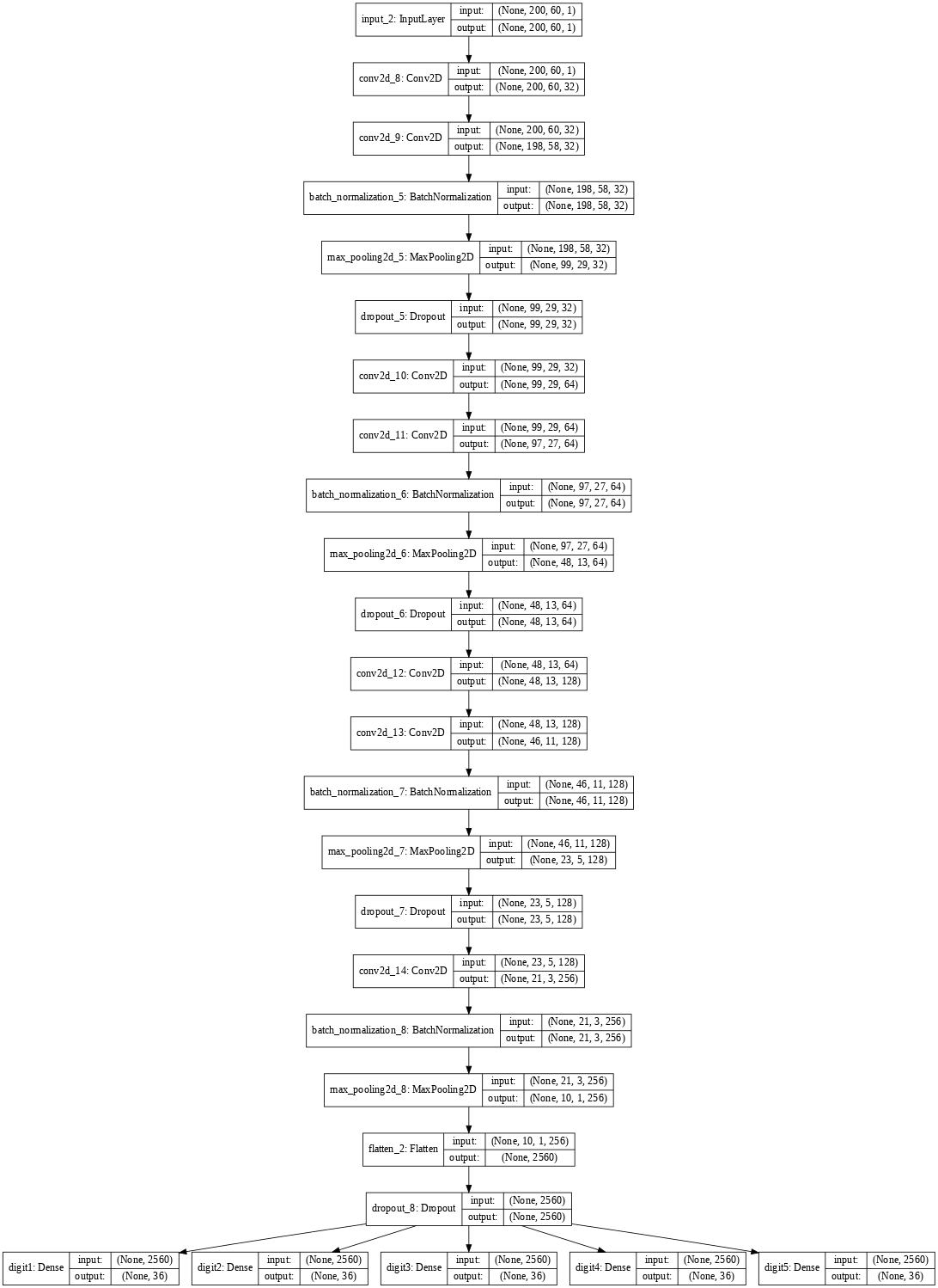
Figure 14.19: Our vanilla model for cracking 5-letter railway CAPTCHA.

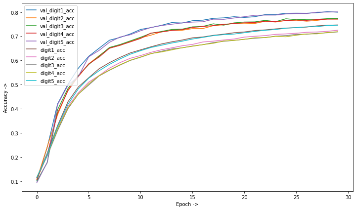
Figure 14.20: Training Accuracy for our vanilla model (14.19).

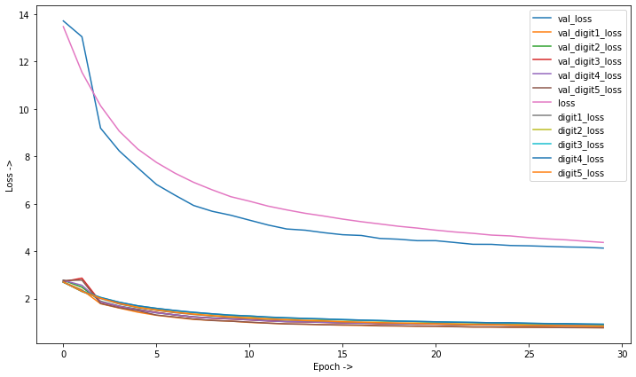
Figure 14.22: Training Loss for the vanilla model (14.19).

We then checked how the same model performs with CAPTCHAs generated from the same dataset but this time with 5-character length labels. Here, the size and dimensions of the image are same as the previous one, the pre-processing done on the image is same too. We just changed some of the output nodes of the model and checked how this performed. The summary of the model is shown in Figure 14.16. The summary of the epochs is shown in Figure 14.17. It takes about 83 seconds to complete one epoch and a total of 41.5 minutes to finish the training. The graph layout of the model is shown in Figure 14.19. The accuracy obtained is about 77% and the plot is shown in Figure 14.20. The trained model can be retrieved from this url (https://jimut123.github.io/blogs/CAPTCHA/models/railway_captcha_5_imop.h5). The plot for the loss for the same model is shown in Figure 14.22. When the model is tested on real world unseen data, we get the prediction of 14.23, which shows that the performance is not so well on real world data. The model predicts 23 images wrongly out of 36 images which is way more less than human level operator.

⬇

__________________________________________________________________________________________________

Layer (type) Output Shape Param # Connected to

==================================================

input_1 (InputLayer) (None, 200, 60, 1) 0

__________________________________________________________________________________________________

conv2d_1 (Conv2D) (None, 200, 60, 32) 320 input_1[0][0]

__________________________________________________________________________________________________

conv2d_2 (Conv2D) (None, 198, 58, 32) 9248 conv2d_1[0][0]

__________________________________________________________________________________________________

batch_normalization_1 (BatchNor (None, 198, 58, 32) 128 conv2d_2[0][0]

__________________________________________________________________________________________________

max_pooling2d_1 (MaxPooling2D) (None, 99, 29, 32) 0 batch_normalization_1[0][0]

__________________________________________________________________________________________________

dropout_1 (Dropout) (None, 99, 29, 32) 0 max_pooling2d_1[0][0]

__________________________________________________________________________________________________

conv2d_3 (Conv2D) (None, 99, 29, 64) 18496 dropout_1[0][0]

__________________________________________________________________________________________________

conv2d_4 (Conv2D) (None, 97, 27, 64) 36928 conv2d_3[0][0]

__________________________________________________________________________________________________

batch_normalization_2 (BatchNor (None, 97, 27, 64) 256 conv2d_4[0][0]

__________________________________________________________________________________________________

max_pooling2d_2 (MaxPooling2D) (None, 48, 13, 64) 0 batch_normalization_2[0][0]

__________________________________________________________________________________________________

dropout_2 (Dropout) (None, 48, 13, 64) 0 max_pooling2d_2[0][0]

__________________________________________________________________________________________________

conv2d_5 (Conv2D) (None, 48, 13, 128) 73856 dropout_2[0][0]

__________________________________________________________________________________________________

conv2d_6 (Conv2D) (None, 46, 11, 128) 147584 conv2d_5[0][0]

__________________________________________________________________________________________________

batch_normalization_3 (BatchNor (None, 46, 11, 128) 512 conv2d_6[0][0]

__________________________________________________________________________________________________

max_pooling2d_3 (MaxPooling2D) (None, 23, 5, 128) 0 batch_normalization_3[0][0]

__________________________________________________________________________________________________

dropout_3 (Dropout) (None, 23, 5, 128) 0 max_pooling2d_3[0][0]

__________________________________________________________________________________________________

conv2d_7 (Conv2D) (None, 21, 3, 256) 295168 dropout_3[0][0]

__________________________________________________________________________________________________

batch_normalization_4 (BatchNor (None, 21, 3, 256) 1024 conv2d_7[0][0]

__________________________________________________________________________________________________

max_pooling2d_4 (MaxPooling2D) (None, 10, 1, 256) 0 batch_normalization_4[0][0]

__________________________________________________________________________________________________

flatten_1 (Flatten) (None, 2560) 0 max_pooling2d_4[0][0]

__________________________________________________________________________________________________

dropout_4 (Dropout) (None, 2560) 0 flatten_1[0][0]

__________________________________________________________________________________________________

digit1 (Dense) (None, 36) 87074 dropout_4[0][0]

__________________________________________________________________________________________________

digit2 (Dense) (None, 36) 87074 dropout_4[0][0]

__________________________________________________________________________________________________

digit3 (Dense) (None, 36) 87074 dropout_4[0][0]

__________________________________________________________________________________________________

digit4 (Dense) (None, 36) 87074 dropout_4[0][0]

__________________________________________________________________________________________________

digit5 (Dense) (None, 36) 87074 dropout_4[0][0]

==================================================

Total params: 1,018,890

Trainable params: 1,017,930

Non-trainable params: 960

__________________________________________________________________________________________________

Figure 14.16: Model (14.19) Summary.

⬇

Epoch 30/30

72000/72000 [==============================] - 83s 1ms/step - loss: 4.3662 - digit1_loss: 0.8213 - digit2_loss: 0.8910 - digit3_loss: 0.9141 - digit4_loss: 0.9161 - digit5_loss: 0.8237 - digit1_acc: 0.7472 - digit2_acc: 0.7252 - digit3_acc: 0.7183 - digit4_acc: 0.7191 - digit5_acc: 0.7460 - val_loss: 4.1281 - val_digit1_loss: 0.7711 - val_digit2_loss: 0.8651 - val_digit3_loss: 0.8587 - val_digit4_loss: 0.8666 - val_digit5_loss: 0.7666 - val_digit1_acc: 0.7996 - val_digit2_acc: 0.7713 - val_digit3_acc: 0.7741 - val_digit4_acc: 0.7713 - val_digit5_acc: 0.8012

Figure 14.17: Summary for model’s (14.19) epochs

⬇

Epoch 30/30

72000/72000 [==============================] - 95s 1ms/step - loss: 5.9938 - digit1_loss: 0.8645 - digit2_loss: 1.0304 - digit3_loss: 1.1001 - digit4_loss: 1.0711 - digit5_loss: 1.0102 - digit6_loss: 0.9174 - digit1_acc: 0.7351 - digit2_acc: 0.6786 - digit3_acc: 0.6537 - digit4_acc: 0.6624 - digit5_acc: 0.6869 - digit6_acc: 0.7162 - val_loss: 5.3350 - val_digit1_loss: 0.7786 - val_digit2_loss: 0.9233 - val_digit3_loss: 0.9596 - val_digit4_loss: 0.9521 - val_digit5_loss: 0.9080 - val_digit6_loss: 0.8133 - val_digit1_acc: 0.7951 - val_digit2_acc: 0.7558 - val_digit3_acc: 0.7511 - val_digit4_acc: 0.7475 - val_digit5_acc: 0.7544 - val_digit6_acc: 0.7829

Figure 14.18: Summary for model’s (14.25) epochs

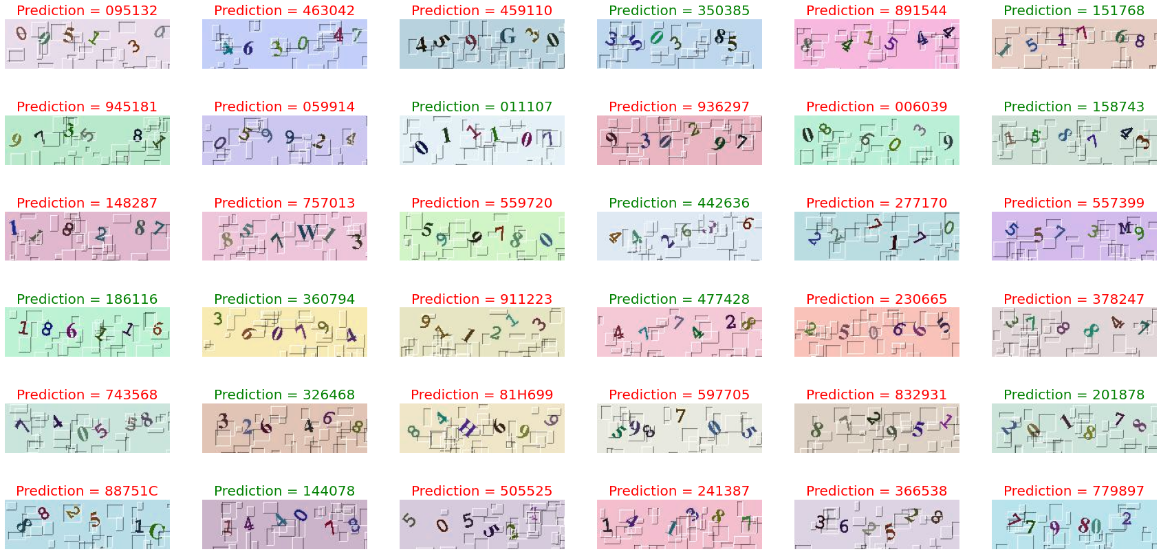
Figure 14.21: Predictions of the vanilla model (14.25).

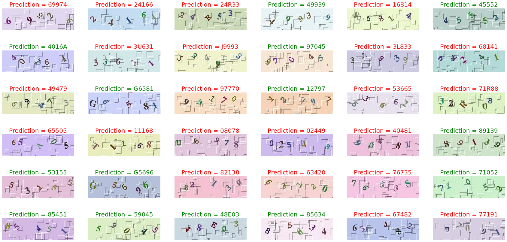
Figure 14.23: Predictions of the vanilla model (14.19).

14.4 Railway-CAPTCHA with 6 Letters

We then checked how the same model performs with CAPTCHAs generated from the same dataset but this time with 6-character length labels. Here, the size and dimensions of the image are same as the previous one, the pre-processing done on the image is same too. We just changed some of the output nodes of the model and checked how this performed. The summary of the model is shown in Figure 14.24. The summary of the epochs is shown in Figure 14.18. It takes about 83 seconds to complete one epoch and a total of 41.5 minutes to finish the training. The graph layout of the model is shown in Figure 14.25. The same layout when visualized in tensorboard is shown in Figure 14.28. The accuracy obtained is about 77% and the plot is shown in Figure 14.26. The trained model can be retrieved from this url (https://jimut123.github.io/blogs/CAPTCHA/models/railway_captcha_6_imop.h5). The plot for the loss for the same model is shown in Figure 14.27. When the model is tested on real world unseen data, we get the prediction of 14.21, which shows that the performance is not so well on real world data. The model predicts 25 images wrongly out of 36 images which is way less than human level operator.

⬇

Layer (type) Output Shape Param # Connected to

==================================================

input_1 (InputLayer) (None, 200, 60, 1) 0

__________________________________________________________________________________________________

conv2d_1 (Conv2D) (None, 200, 60, 32) 320 input_1[0][0]

__________________________________________________________________________________________________

conv2d_2 (Conv2D) (None, 198, 58, 32) 9248 conv2d_1[0][0]

__________________________________________________________________________________________________

batch_normalization_1 (BatchNor (None, 198, 58, 32) 128 conv2d_2[0][0]

__________________________________________________________________________________________________

max_pooling2d_1 (MaxPooling2D) (None, 99, 29, 32) 0 batch_normalization_1[0][0]

__________________________________________________________________________________________________

dropout_1 (Dropout) (None, 99, 29, 32) 0 max_pooling2d_1[0][0]

__________________________________________________________________________________________________

conv2d_3 (Conv2D) (None, 99, 29, 64) 18496 dropout_1[0][0]

__________________________________________________________________________________________________

conv2d_4 (Conv2D) (None, 97, 27, 64) 36928 conv2d_3[0][0]

__________________________________________________________________________________________________

batch_normalization_2 (BatchNor (None, 97, 27, 64) 256 conv2d_4[0][0]

__________________________________________________________________________________________________

max_pooling2d_2 (MaxPooling2D) (None, 48, 13, 64) 0 batch_normalization_2[0][0]

__________________________________________________________________________________________________

dropout_2 (Dropout) (None, 48, 13, 64) 0 max_pooling2d_2[0][0]

__________________________________________________________________________________________________

conv2d_5 (Conv2D) (None, 48, 13, 128) 73856 dropout_2[0][0]

__________________________________________________________________________________________________

conv2d_6 (Conv2D) (None, 46, 11, 128) 147584 conv2d_5[0][0]

__________________________________________________________________________________________________

batch_normalization_3 (BatchNor (None, 46, 11, 128) 512 conv2d_6[0][0]

__________________________________________________________________________________________________

max_pooling2d_3 (MaxPooling2D) (None, 23, 5, 128) 0 batch_normalization_3[0][0]

__________________________________________________________________________________________________

dropout_3 (Dropout) (None, 23, 5, 128) 0 max_pooling2d_3[0][0]

__________________________________________________________________________________________________

conv2d_7 (Conv2D) (None, 21, 3, 256) 295168 dropout_3[0][0]

__________________________________________________________________________________________________

batch_normalization_4 (BatchNor (None, 21, 3, 256) 1024 conv2d_7[0][0]

__________________________________________________________________________________________________

max_pooling2d_4 (MaxPooling2D) (None, 10, 1, 256) 0 batch_normalization_4[0][0]

__________________________________________________________________________________________________

flatten_1 (Flatten) (None, 2560) 0 max_pooling2d_4[0][0]

__________________________________________________________________________________________________

dropout_4 (Dropout) (None, 2560) 0 flatten_1[0][0]

__________________________________________________________________________________________________

digit1 (Dense) (None, 36) 87074 dropout_4[0][0]

__________________________________________________________________________________________________

digit2 (Dense) (None, 36) 87074 dropout_4[0][0]

__________________________________________________________________________________________________

digit3 (Dense) (None, 36) 87074 dropout_4[0][0]

__________________________________________________________________________________________________

digit4 (Dense) (None, 36) 87074 dropout_4[0][0]

__________________________________________________________________________________________________

digit5 (Dense) (None, 36) 87074 dropout_4[0][0]

__________________________________________________________________________________________________

digit6 (Dense) (None, 36) 87074 dropout_4[0][0]

==================================================

Total params: 1,105,964

Trainable params: 1,105,004

Non-trainable params: 960

__________________________________________________________________________________________________

Figure 14.24: Model (14.25) Summary.

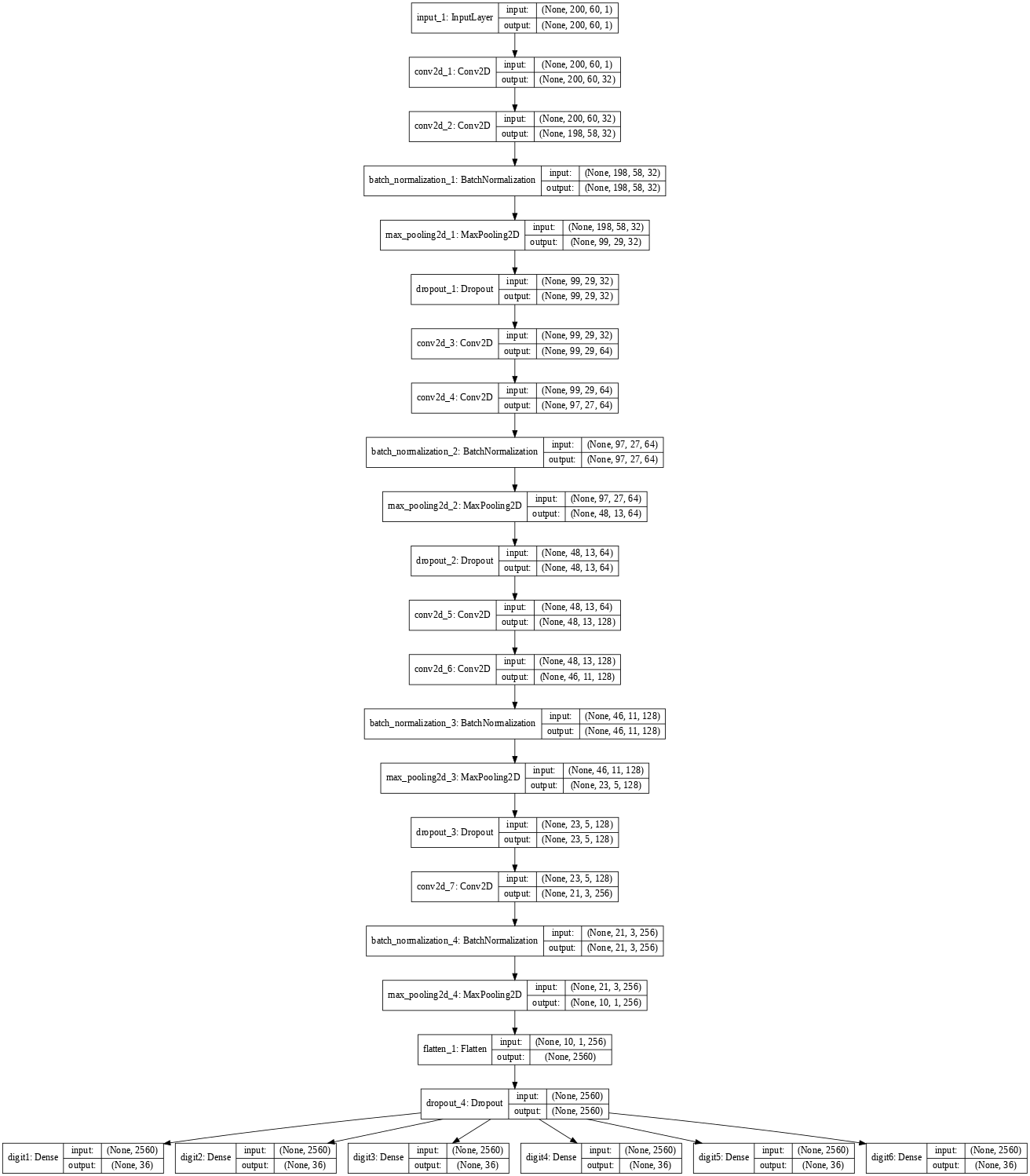
Figure 14.25: Our vanilla model for cracking 6-letter railway CAPTCHA.

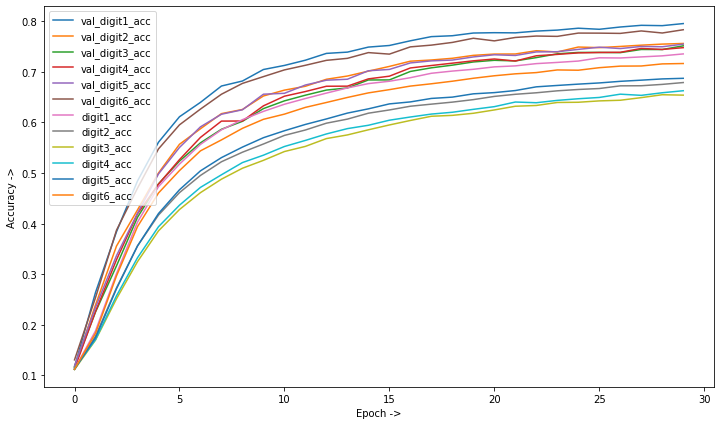
Figure 14.26: Training Accuracy for vanilla model (14.25).

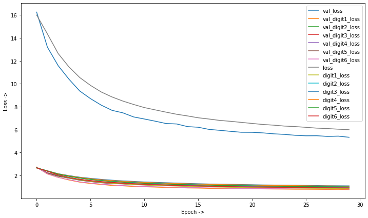
Figure 14.27: Training Loss for vanilla model (14.25).

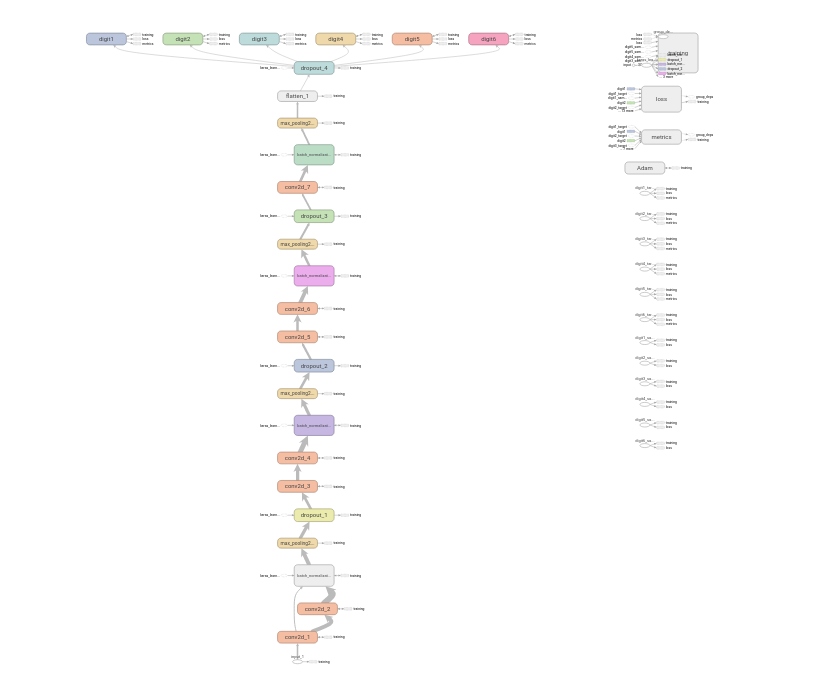
Figure 14.28: Model’s graph as visualized in tensorboard (14.25).

14.5 Railway-CAPTCHA with 7 Letters

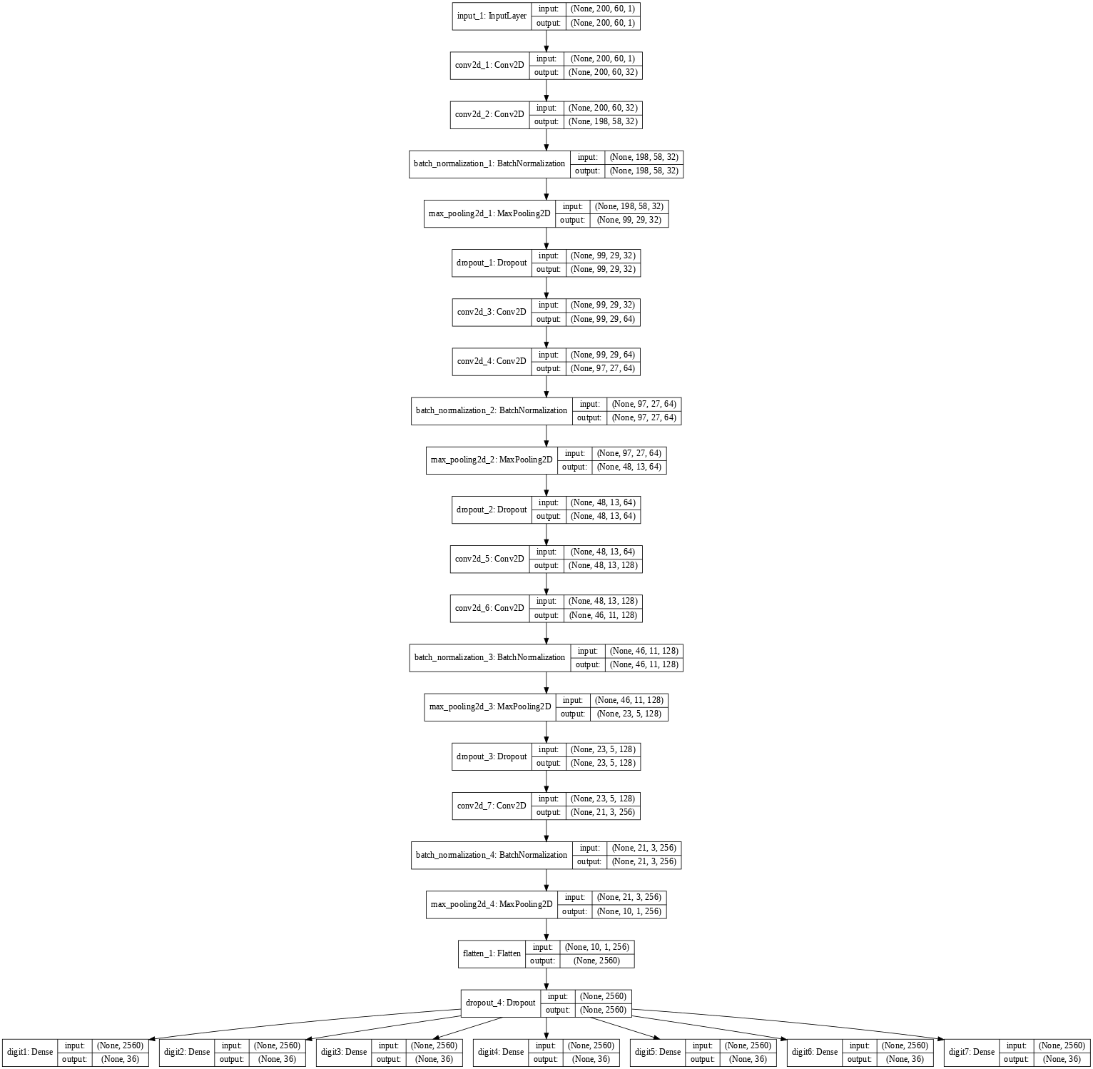
Figure 14.32: Our vanilla model for cracking 7-letter railway CAPTCHA.

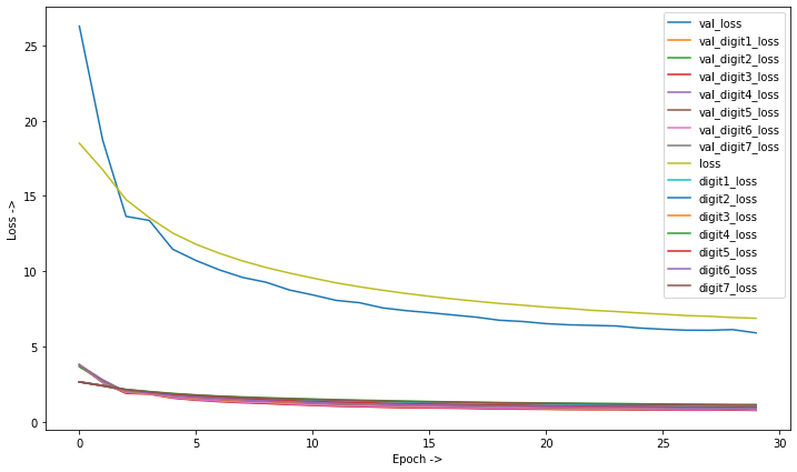
Figure 14.34: Training Loss for vanilla model (14.32).

We then checked how the same model performs with CAPTCHAs generated from the same dataset but this time with 7-character length labels. Here, the size and dimensions of the image are same as the previous one, the pre-processing done on the image is same too. We just changed some of the output nodes of the model and checked how this performed. The summary of the model is shown in Figure 14.29. The summary of the epochs is shown in Figure 14.30. It takes about 91 seconds to complete one epoch and a total of 45.5 minutes to finish the training. The graph layout of the model is shown in Figure 14.32. The accuracy obtained is about 75% and the plot is shown in Figure 14.26. The trained model can be retrieved from this url (https://jimut123.github.io/blogs/CAPTCHA/models/railway_captcha_7_imop.h5). The plot for the loss for the same model is shown in Figure 14.34. When the model is tested on real world unseen data, we get the prediction of 14.35, which shows that the performance is not at all well on real world data. The model predicts 36 images wrongly out of 36 images which is naive.

⬇

__________________________________________________________________________________________________

Layer (type) Output Shape Param # Connected to

==================================================

input_1 (InputLayer) (None, 200, 60, 1) 0

__________________________________________________________________________________________________

conv2d_1 (Conv2D) (None, 200, 60, 32) 320 input_1[0][0]

__________________________________________________________________________________________________

conv2d_2 (Conv2D) (None, 198, 58, 32) 9248 conv2d_1[0][0]

__________________________________________________________________________________________________

batch_normalization_1 (BatchNor (None, 198, 58, 32) 128 conv2d_2[0][0]

__________________________________________________________________________________________________

max_pooling2d_1 (MaxPooling2D) (None, 99, 29, 32) 0 batch_normalization_1[0][0]

__________________________________________________________________________________________________

dropout_1 (Dropout) (None, 99, 29, 32) 0 max_pooling2d_1[0][0]

__________________________________________________________________________________________________

conv2d_3 (Conv2D) (None, 99, 29, 64) 18496 dropout_1[0][0]

__________________________________________________________________________________________________

conv2d_4 (Conv2D) (None, 97, 27, 64) 36928 conv2d_3[0][0]

__________________________________________________________________________________________________

batch_normalization_2 (BatchNor (None, 97, 27, 64) 256 conv2d_4[0][0]

__________________________________________________________________________________________________

max_pooling2d_2 (MaxPooling2D) (None, 48, 13, 64) 0 batch_normalization_2[0][0]

__________________________________________________________________________________________________

dropout_2 (Dropout) (None, 48, 13, 64) 0 max_pooling2d_2[0][0]

__________________________________________________________________________________________________

conv2d_5 (Conv2D) (None, 48, 13, 128) 73856 dropout_2[0][0]

__________________________________________________________________________________________________

conv2d_6 (Conv2D) (None, 46, 11, 128) 147584 conv2d_5[0][0]

__________________________________________________________________________________________________

batch_normalization_3 (BatchNor (None, 46, 11, 128) 512 conv2d_6[0][0]

__________________________________________________________________________________________________

max_pooling2d_3 (MaxPooling2D) (None, 23, 5, 128) 0 batch_normalization_3[0][0]

__________________________________________________________________________________________________

dropout_3 (Dropout) (None, 23, 5, 128) 0 max_pooling2d_3[0][0]

__________________________________________________________________________________________________

conv2d_7 (Conv2D) (None, 21, 3, 256) 295168 dropout_3[0][0]

__________________________________________________________________________________________________

batch_normalization_4 (BatchNor (None, 21, 3, 256) 1024 conv2d_7[0][0]

__________________________________________________________________________________________________

max_pooling2d_4 (MaxPooling2D) (None, 10, 1, 256) 0 batch_normalization_4[0][0]

__________________________________________________________________________________________________

flatten_1 (Flatten) (None, 2560) 0 max_pooling2d_4[0][0]

__________________________________________________________________________________________________

dropout_4 (Dropout) (None, 2560) 0 flatten_1[0][0]

__________________________________________________________________________________________________

digit1 (Dense) (None, 36) 92196 dropout_4[0][0]

__________________________________________________________________________________________________

digit2 (Dense) (None, 36) 92196 dropout_4[0][0]

__________________________________________________________________________________________________

digit3 (Dense) (None, 36) 92196 dropout_4[0][0]

__________________________________________________________________________________________________

digit4 (Dense) (None, 36) 92196 dropout_4[0][0]

__________________________________________________________________________________________________

digit5 (Dense) (None, 36) 92196 dropout_4[0][0]

__________________________________________________________________________________________________

digit6 (Dense) (None, 36) 92196 dropout_4[0][0]

__________________________________________________________________________________________________

digit7 (Dense) (None, 36) 92196 dropout_4[0][0]

==================================================

Total params: 1,228,892

Trainable params: 1,227,932

Non-trainable params: 960

__________________________________________________________________________________________________

Figure 14.29: Model (14.32) Summary.

⬇

Epoch 25/30

72000/72000 [==============================] - 91s 1ms/step - loss: 7.2219 - digit1_loss: 1.1113 - digit2_loss: 0.9235 - digit3_loss: 0.9135 - digit4_loss: 1.1867 - digit5_loss: 0.9920 - digit6_loss: 0.9389 - digit7_loss: 1.1559 - digit1_acc: 0.6421 - digit2_acc: 0.7140 - digit3_acc: 0.7157 - digit4_acc: 0.6182 - digit5_acc: 0.6900 - digit6_acc: 0.7096 - digit7_acc: 0.6248 - val_loss: 6.2208 - val_digit1_loss: 0.9165 - val_digit2_loss: 0.8048 - val_digit3_loss: 0.7847 - val_digit4_loss: 1.0185 - val_digit5_loss: 0.8535 - val_digit6_loss: 0.8239 - val_digit7_loss: 1.0190 - val_digit1_acc: 0.7541 - val_digit2_acc: 0.7892 - val_digit3_acc: 0.7947 - val_digit4_acc: 0.7192 - val_digit5_acc: 0.7763 - val_digit6_acc: 0.7780 - val_digit7_acc: 0.7152

Figure 14.30: Summary for model’s (14.32) epochs

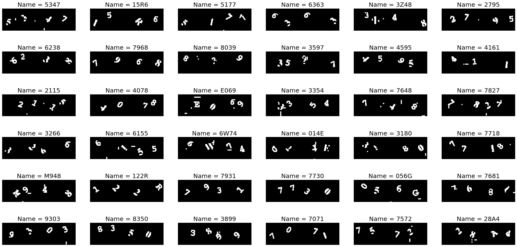
Figure 14.31: A subset of samples given to the model (14.10)

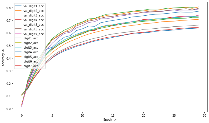
Figure 14.33: Training Accuracy for vanilla model (14.32).

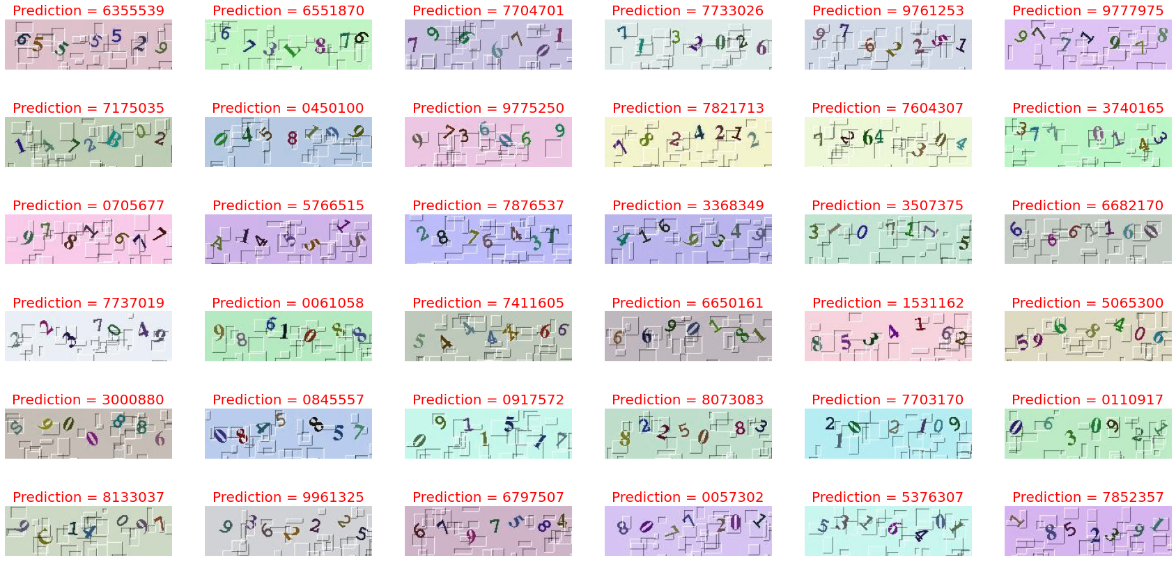
Figure 14.35: Predictions of the model (14.32).

14.6 What possibly went wrong?

We can see that the sample of images when preprocessed, before passing to the model has a lot of clutter in them as shown in Figure 14.31. From studies [8] we know that even a single pixel can change the output of the prediction by a vast amount. There were more to the existing problem of clutter and occlusion. When we saw the distribution of the dataset’s character labels, we found that though it was generated randomly, it followed a certain trend. The labels for the dataset for 3 letters have characters 0-9 ten times more often than the other letter ranging from A to Z. Similarly, for other datasets. This might be due to the anomaly in clock speed and internal problem of pipelining and parallel execution of CPU of the machine in which it was generated. This leads to the bias for not learning the A-Z characters as good as 0-9 letters. So, we need to generate a brute force algorithm for generation of uniformly distributed character data. We first thought of brute forcing the labels and generating data like the output produced by the famous software crunch for brute forcing passwords, but it is too naive and the number of labels would increase exponentially with the number of characters in the labels. We can think of an algorithm which will initialize the distribution and select the labels randomly deducting each label generated from the initial list of the labels.

 

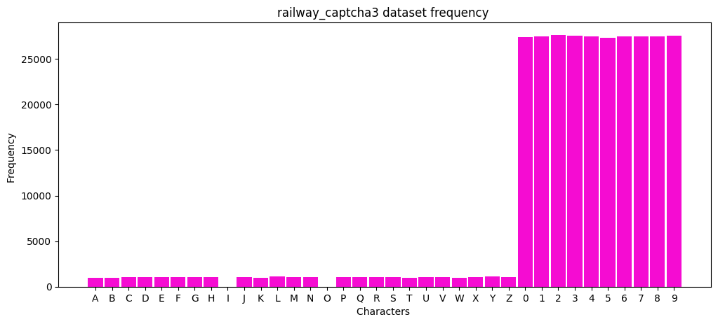
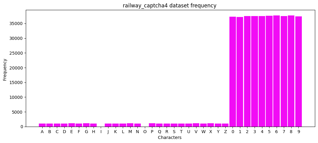
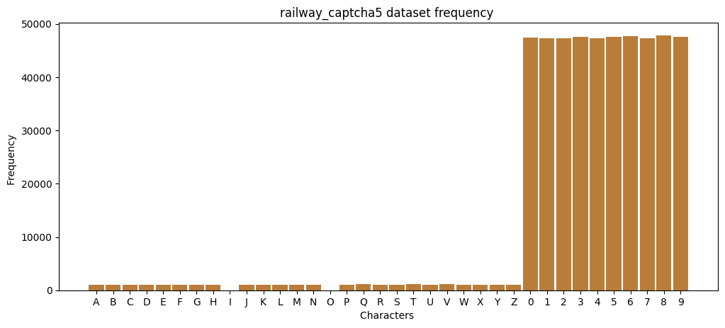
Figure 14.36: Distribution of the data for the various labels of the Railway CAPTCHA dataset for (3,4 and 5 letter images).

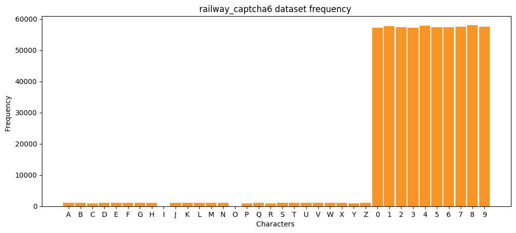
Figure 14.37: Distribution of the data for the various labels of the Railway CAPTCHA dataset (for 6 and 7 letter images).

14.7 What can we conclude from this?

It is sure from the behavior of the model that as the number of letters in the CAPTCHA increases, the complexity of the CAPTCHA increases. This is good for designing better CAPTCHAs since for humans, it is very easy task to solve long paragraphs of simple writing than to solve few sentences of obfuscated writing. The overall accuracy of the model might decrease significantly as shown in Table 14.1 and Figure 14.38. The figure and the information in the table shows that the complexity of the model increases linearly with the increase in number of letters in CAPTCHA. In a multi label classification this reduces drastically, since the complexity of the model would also increase. In case of multi-class classification where each character is segmented and predicted, it will also become difficult for the machine learning algorithm to solve and decipher large texts of huge data. Since the CAPTCHA is said to be correct when each and every letter of the CAPTCHA is correctly classified, in any case each segmented character receives an accuracy of classification of about 95 % then if there are about 10 letter then the total accuracy of correct classification becomes (95)¹⁰ which is 59.87%. This shows that the complexity for CAPTCHAs to the computers can be increased significantly. So, we conjecture that long length CAPTCHA are better solution to hard games which are not easy to understand at first glance, and takes a reasonable amount of time in determining the moves for genuine users.

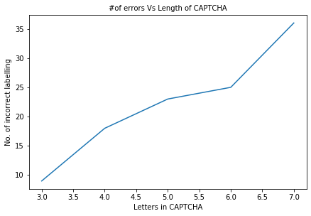
Figure 14.38: The complexity of the model increases with the length of the CAPTCHA, data from table (14.1).

No. of letters	No. of incorrect labelling	Accuracy (in %)
3	9	80
4	18	79
5	23	77
6	25	77
7	36	75

Table 14.1: Table showing that the length of the CAPTCHA is directly proportional to the complexity.

Chapter 15 Conclusions

This investigation resulted in successfully breaking most of the text CAPTCHA’s with human level accuracy. This means that the text CAPTCHA’s are not so much reliable to predict whether a user is a human or not. We have also shown that if we increase the size of the length of labels in the CAPTCHA, then it might be difficult for computers to break them with human level accuracy. When we want to have state of the art accuracy in deciphering complex CAPTCHAs with multi-label classification, then it is necessary to have a large number of data [9]. If the number of parameters in the neural network is $P$, then it is always a good rule of thumb to have $P^{2}$ amount of data points. We have also seen that when a simple model can give state of the art accuracy as compared to a complex model, we will stick to a simple model since that will give a good generalization of the data without overfitting much (by Occam’s razor). It is also good to visualize what we are trying to achieve at every step to get to the point where we can do better, to give us direction towards achieving good accuracy with models.

We have also seen that in case of training deep neural networks, data augmentation is necessary since it might not be the case that we are getting so much amount of data, and performing some basic image processing tasks to augment the data always helps. It is also known that there is no convergence proof for deep neural networks, so it is astonishing that they perform so well when the amount of data increases and sometimes performs better than humans. The successful completion of this project will enhance the way raw text image is classified for data retrieval from web search queries. Converting images containing text to actual text can give rise to efficient algorithm for web search queries, where it is difficult to search for images by certain text when they are unlabeled.

It is also seen that dropouts helps in training ensemble of networks which helps in reducing noise and generalizing well on unseen data. The main motive of the project was to create a generic CAPTCHA solver, and the AlexNet type model with multilabel classification and a dropout before the final layer helps to generalize well on the unseen data, which gives almost human level accuracy. We have also seen that when the data is less, we need to feed the whole of the dataset with augmentations, if necessary, we need to give 3 channels if there is a lot of noise in the image data. This will help the network learn the important features all by itself.

It is well known that text CAPTCHA is getting away and some new types of creative CAPTCHAs are coming day by day. We have seen that there has been gaming CAPTCHA, puzzle CAPTCHA, voice CAPTCHA as shown in Figure 1.2. These types of CAPTCHAs are more challenging to solve than text CAPTCHA and particular puzzle needs particular type of architecture to solve. Google reCAPTCHA v3 uses advanced cookie system to check if the user is a bot or not. These types of techniques to determine the authenticity of users are emerging which induces less pain to solve and crack CAPTCHA every day. So, indeed text-based CAPTCHA is a week type of CAPTCHA.

15.1 Future Work

This project, though is the beginning of obfuscated Optical Character Recognition, can be well suited in future for the digital conversion of large corpus of Handwritten datasets. One example of such a dataset can be IAM Handwriting Database. Though the claim of future work will be highly dramatic like classifying a huge corpus of text by segmentation procedures and converting each digital image found on internet to its corresponding text which will help in information retrieval and segregating data in their own form. It can also be used to segment huge database of handwritten documents which are not yet converted to digital text due to lack of human resources. Another typical future work will be to find text in unconstrained environments which will help to detect license plate with high accuracy. It may also be used for converting handwritten test papers to digit copy for preservation, and maybe some AI to auto check all the test papers in some huge test. Converting handwritten text to digital text is one of the most challenging tasks in computer vision since the data needs to be generalized on a wide variety of lighting conditions at different scales and a lot of different types of handwriting. This makes the problem even harder, since it is not possible to get all the handwriting styles for such a wide diversity of people.

[Keyword]

Appendix A Appendix

A.1 Softwares Used

We have extensively used Keras, which is open source library capable of running on top of tensorflow. We have used tensorflow as backend. We have used matplotlib and plotly for generating graphs and plots used in this documentation. We have used Google’s Colaboratory’s GPU power extensively. We have created the projects and dataset in such a way that they can be easily run in cloud. There were various animations that were generated during this project. We have used figshare to host the data, so that they can be easily fetched from cloud without any token or certificates. We have also used https://alexlenail.me/NN-SVG/ to create the models in 3D. The last picture in the thesis is captured by me.

A.2 Dataset and Model generated

Here, we will share the datasets and model that were generated and created by us during the course of this project.

Captcha (4 letter) : dataset can be found here https://jimut123.github.io/blogs/CAPTCHA/data/captcha_4_letter.tar.gz and the model for this dataset can be obtained from here https://jimut123.github.io/blogs/CAPTCHA/models/captcha_4_letter_our_model.h5.

c4l_16x16_550: dataset can be found here https://jimut123.github.io/blogs/CAPTCHA/data/c4l-16x16_550.tar.gz and the model for this dataset can be obtained from here https://jimut123.github.io/blogs/CAPTCHA/models/CNN_c4l-16x16_550.h5.

resized_JAM: dataset can be found here https://jimut123.github.io/blogs/CAPTCHA/data/resized_JAM.tar.gz. The model used was k-NN and it can be easily formed without any computationally expensive training.

CAPTCHA-version-2: dataset can be found here https://jimut123.github.io/blogs/CAPTCHA/data/captcha_v2.tar.gz and the model for this dataset can be obtained from here https://jimut123.github.io/blogs/CAPTCHA/models/captcha_v2_alexNet.h5 and here https://jimut123.github.io/blogs/CAPTCHA/models/captcha_v2_1_drive.h5.

100000-labeled-captchas: dataset can be found here https://dx.doi.org/10.6084/m9.figshare.12046881.v1 and the model for this dataset can be obtained from here https://jimut123.github.io/blogs/CAPTCHA/models/images-1L-processed.h5.

Faded CAPTCHA data. The faded CAPTCHA dataset is comprised of about 3.7 GiB data files in total. It is partitioned into folders and uploaded to figshare. The dataset can be found from these links:

https://dx.doi.org/10.6084/m9.figshare.12115656,
https://dx.doi.org/10.6084/m9.figshare.12115671,
https://dx.doi.org/10.6084/m9.figshare.12115689,
https://dx.doi.org/10.6084/m9.figshare.12118302,
https://dx.doi.org/10.6084/m9.figshare.12118371,
https://dx.doi.org/10.6084/m9.figshare.12118482,
https://dx.doi.org/10.6084/m9.figshare.12118836,
https://dx.doi.org/10.6084/m9.figshare.12122853,
https://dx.doi.org/10.6084/m9.figshare.12122934, and
https://dx.doi.org/10.6084/m9.figshare.12122967. The model obtained from the dataset can be found from here https://jimut123.github.io/blogs/CAPTCHA/models/faded_captcha.h5.

Railway CAPTCHA
Railway CAPTCHA 3 Letters: dataset can be found from https://dx.doi.org/10.6084/m9.figshare.12045249.v1, and the model for this dataset can be obtained from here https://jimut123.github.io/blogs/CAPTCHA/models/railway_captcha_3.h5.

Railway CAPTCHA 4 Letters: dataset can be found from https://dx.doi.org/10.6084/m9.figshare.12045288.v1, and the model for this dataset can be obtained from here https://jimut123.github.io/blogs/CAPTCHA/models/railway_captcha_4.h5.

Railway CAPTCHA 5 Letters: dataset can be found from https://dx.doi.org/10.6084/m9.figshare.12045294.v1, and the model for this dataset can be obtained from here https://jimut123.github.io/blogs/CAPTCHA/models/railway_captcha_5.h5.

Railway CAPTCHA 6 Letters: dataset can be found from https://dx.doi.org/10.6084/m9.figshare.12045657.v1, and the model for this dataset can be obtained from here https://jimut123.github.io/blogs/CAPTCHA/models/railway_captcha_6.h5.

Railway CAPTCHA 7 Letters: dataset can be found from https://dx.doi.org/10.6084/m9.figshare.12053937.v1, and the model for this dataset can be obtained from here https://jimut123.github.io/blogs/CAPTCHA/models/railway_captcha_7.h5.

Circle CAPTCHA: dataset can be found here https://figshare.com/articles/captcha_gen/12286766 and the model for this dataset can be obtained from here (https://jimut123.github.io/blogs/CAPTCHA/models/circle_captcha_10e.h5).

Sphinx CAPTCHA (4 letters): There are 34 pieces of tar.gz files that are found over figshare and zenodo (due to some problem during the CoviD-19 crisis in figshare). The whole dataset can be found from here:

https://ndownloader.figshare.com/files/22336164,
https://ndownloader.figshare.com/files/22344408,
https://ndownloader.figshare.com/files/22366674,
https://ndownloader.figshare.com/files/22367007,
https://ndownloader.figshare.com/files/22388370,
https://ndownloader.figshare.com/files/22388556,
https://ndownloader.figshare.com/files/22399503,
https://ndownloader.figshare.com/files/22399554,
https://ndownloader.figshare.com/files/22414872,
https://zenodo.org/record/3782676/files/sphinx_010.tar.gz?download=1,
https://ndownloader.figshare.com/files/22477673,
https://ndownloader.figshare.com/files/22477823,
https://zenodo.org/record/3782690/files/sphinx_013.tar.gz?download=1,
https://zenodo.org/record/3782704/files/sphinx_014.tar.gz?download=1,
https://zenodo.org/record/3782733/files/sphinx_015.tar.gz?download=1,
https://zenodo.org/record/3783674/files/sphinx_016.tar.gz?download=1,
https://zenodo.org/record/3783691/files/sphinx_017.tar.gz?download=1,
https://zenodo.org/record/3785093/files/sphinx_018.tar.gz?download=1,
https://ndownloader.figshare.com/files/22533749,
https://ndownloader.figshare.com/files/22533821,
https://ndownloader.figshare.com/files/22533965,
https://ndownloader.figshare.com/files/22534058,
https://ndownloader.figshare.com/files/22542704,
https://ndownloader.figshare.com/files/22542782,
https://ndownloader.figshare.com/files/22542851,
https://ndownloader.figshare.com/files/22542944,
https://ndownloader.figshare.com/files/22543832,
https://ndownloader.figshare.com/files/22543850,
https://ndownloader.figshare.com/files/22543979,
https://ndownloader.figshare.com/files/22584218,
https://ndownloader.figshare.com/files/22585160,
https://ndownloader.figshare.com/files/22621634,
https://ndownloader.figshare.com/files/22621694, and
https://ndownloader.figshare.com/files/22624358. The total dataset comprise of about 12.2 GB and the model for this dataset can be obtained from here (https://jimut123.github.io/blogs/CAPTCHA/models/sphinx_full_34_15e_9962.h5).

Fish eye CAPTCHA: dataset can be found from https://figshare.com/articles/Fish_Eye/12235946. The dataset contains 8 pieces of zip folders which can be further extracted to obtain the actual dataset. The trained model can be obtained from the following link (https://jimut123.github.io/blogs/CAPTCHA/models/fish_eye.h5).

Mini CAPTCHA: dataset can be found from https://figshare.com/articles/Mini_Captcha/12286697. The dataset contains 8 pieces of zip folders which can be further extracted to obtain the actual dataset. The trained model can be obtained from the following link (https://drive.google.com/open?id=1w5BhaeSvc1LYQfUuvwBApeNbcx0vkOUP).

Multicolor CAPTCHA: dataset can be found from https://ndownloader.figshare.com/files/22307958,
https://ndownloader.figshare.com/files/22318224,
https://ndownloader.figshare.com/files/22335879,
https://ndownloader.figshare.com/files/22344393,
https://ndownloader.figshare.com/files/22346499,
https://ndownloader.figshare.com/files/22397457,
https://ndownloader.figshare.com/files/22414434,
https://ndownloader.figshare.com/files/22422816,
https://ndownloader.figshare.com/files/22451057, and
https://ndownloader.figshare.com/files/22467227. These contains 10 pieces of tar.gz folders which amount to about 12.7 GiB of tar.gz file. The model that was trained for 10 epochs can be found from this drive link https://drive.google.com/open?id=1-2DW3CBkddRoUsBbaukf7OxR1MZpwVrn. The size of the model is 996 MB.

A.3 Accuracy obtained

The accuracy obtained and their respective CAPTCHA name are described in this section.

Dataset	Note	Accuracy
captcha_4_letter	This is the cleaned version of the dataset obtained from Kaggle, Size = 10.4 MiB, 9955 files of 72x24.	99.81 %
c4l-16x16_550	Extracted characters from Captcha_4_letter dataset, Size = 1.4 MiB, 17600 files of 16x16.	99.91 %
JAM, resized_JAM	JAM has 308 files of 110x40, Size = 101.7KiB. resized_JAM has 1065 files, 65.7KiB	99.53 %
CAPTCHA-version-2	1070 files of 200x50, Size = 21.5 Mib.	90.102%
Circle CAPTCHA	222K files of 35x120, Size = 437.58 Mib.	99.99%
Sphinx CAPTCHA	1 Million files of 437.58, Size = 12.2 GiB.	99.62%
Fish-eye CAPTCHA	2 Million files of 50x200, Size = 9.84 GB.	99.46%
Mini CAPTCHA	1 Million files of 368x159x3, Size = 5.58 GB.	97.25%
Multicolor CAPTCHA	1 Million files of 375x113x3, (used only 50% of the dataset ) Size = 21.5 Mib.	95.69%
faded	Size = 3.7 GiB, 604800 files of 100x120x3 .	99.44 %
1L-labeled-captchas	109,053 files of 200x50. Size = 215.1 MiB	99.67%
Railway CAPTCHA	100K files of 200x60, Sizes = 241.8 MiB, 253.8 MiB, 265.7MiB, 277.4 MiB, 289.1 MiB	80 % 79 % 77 % 77 % 75 %

See pages 1 of back_cover

References

- [1] Wikipedia contributors. Reverse Turing test — Wikipedia, The Free Encyclopedia, . https://en.wikipedia.org/wiki/Reverse_Turing_test2020. last accessed 24-03-2020.
- [2] A. M. TURING, I.—COMPUTING MACHINERY AND INTELLIGENCE, Mind L IX (1950) 433.
- [3] Wikipedia contributors. Turing test — Wikipedia, The Free Encyclopedia, . https://en.wikipedia.org/wiki/Turing_test2020. last accessed 24-03-2020.
- [4] K. Chellapilla, K. Larson, P. Y. Simard, and M. Czerwinski. Building Segmentation Based Human-Friendly Human Interaction Proofs (HIPs), . In H. S. Baird and D. P. Lopresti, editors, Human Interactive Proofs 1Berlin, Heidelberg2005. Springer Berlin Heidelberg.
- [5] N. Otsu, A Threshold Selection Method from Gray-Level Histograms, IEEE Transactions on Systems, Man and Cybernetics 9 (1979) 62.
- [6] L. van der Maaten and G. Hinton, Visualizing Data using t-SNE, Journal of Machine Learning Research 9 (2008) 2579.
- [7] J. B. Pal. A Deeper Look into Hybrid Images, 2020.
- [8] J. Su, D. V. Vargas, and K. Sakurai, One Pixel Attack for Fooling Deep Neural Networks, IEEE Transactions on Evolutionary Computation 23 (2019) 828–841.
- [9] E. D. Sontag. VC Dimension of Neural Networks, . In Neural Networks and Machine Learning 69. Springer1998.