CDM Based Virtual FMCW MIMO Radar Imaging at 79GHz

Abstract

Multiple Input Multiple Output (MIMO) Frequency Modulated Continuous Wave (FMCW) radars operating at 79GHz are compact, light and cost effective devices with low peak-to-average power ratio that have applications in different areas such as automotive industry and Unmanned Arial Vehicle (UAV) based radar imaging. In order to keep the structure small and simple, these radars come with small number of transmitters and receivers. The number of elements can be virtually increased using techniques such as Time Division Multiplexing (TDM), Frequency Division Multiplexing (FDM) or Code Division Multiplexing (CDM) and as a result higher angular resolution can be achieved. Both TDM and FDM based virtual FMCW MIMO radar imaging process have been reported in literature. However, to the best of our knowledge CDM based virtual FMCW MIMO radar has not received any attention. In this paper we will be using an 79GHz FMCW MIMO radar and apply the idea of the CDM method to increase the number of elements virtually which in turn enhances the angular resolution.

I Introduction

The idea of using Time Division Multiplexing (TDM) and Frequency Division Multiplexing (FDM) techniques in Frequency Modulated Continuous Wave (FMCW) Multiple Input Multiple Output (MIMO) radars to effectively increase the number of receive elements has been reported in literature  [1, 2, 3, 4, 5, 6, 7]. Compared to the FDM based virtual FMCW MIMO radar, the TDM based virtual FMCW MIMO radar has simpler structure and higher resolution in range direction. However, since in the TDM based virtual FMCW MIMO radar transmitters transmit at different time slots, therefore, the signal to noise ratio (SNR) is lower compared to the FDM based virtual FMCW MIMO radar in which all the transmitters transmit simultaneously. The lower resolution for the FDM based virtual FMCW MIMO radar comes from the fact that in the FDM based virtual FMCW MIMO radar the whole bandwidth is divided into several pieces to create the orthogonal beams in space. As a result, each transmitter uses only a portion of the whole bandwidth and the range resolution drops. The Code Division Multiplexing (CDM) based virtual FMCW MIMO radar like the TDM based virtual FMCW MIMO radar has a simple structure and since each transmitter utilizes the full bandwidth, hence, the maximum range resolution can be achieved. Yet, since all the transmitters operate simultaneously, therefore, the SNR will be higher than the case of TDM based virtual FMCW MIMO radars. Another great advantage of the CDM based virtual FMCW MIMO radar stems from the fact that by using orthogonal codes for different radars operating in the same neighborhood, the interference among different users can be avoided. Interference avoidance plays an important role in areas such as automotive applications.

In this paper we address the CDM based virtual FMCW MIMO radar imaging. We present the full formulation of the imaging procedure based on the Multiple Signal Classification (MUSIC) algorithm [8, 9]. We also propose a simple method for system calibration at the baseband level. We then use experimental data gathered from a 79GHz FMCW MIMO radar which operates based on CDM method to show the result of the processing. In order to create orthogonal signals based on CDM method we use Walsh codes [10].

The paper is organized as follows. In Section II we present the problem formulation. We address the system calibration at the baseband level in Section III. We will then apply MUSIC technique for image reconstruction in Section IV. Finally, We have dedicated Section V to the results of applying the algorithm presented in Section IV to the experimental data gathered from a 79GHz CDM based virtual FMCW MIMO radar.

II System Model

The signal transmitted by the $m^{\rm th}$ transmitter and received at the location of the $n^{\rm th}$ receiver after hitting the $l^{\rm th}$ target, is a chirp signal modeled as follows,

$$s^{(l)}_{mn}(t)=\sigma_{l}\;e^{\displaystyle j2\pi f_{c}(t-\tau_{mnl})+j\pi\beta{(t-\tau_{mnl})}^{2}},$$ (1)

where $f_{c}$ is the carrier frequency and $\sigma_{l}$ is the radar cross section for the $l^{\rm th}$ target. The parameter $\beta$ is given as $b/T$, where $b$ and $T$ stand for the bandwidth and the chirp time, respectively. Finally, $\tau_{mn}$ is the time delay for the signal to travel from the $m^{\rm th}$ transmitter and be received at the location of the $n^{\rm th}$ receiver after bouncing off the $l^{\rm th}$ target.

Fig. 1 shows the idea behind virtual MIMO radar based on the CDM method.

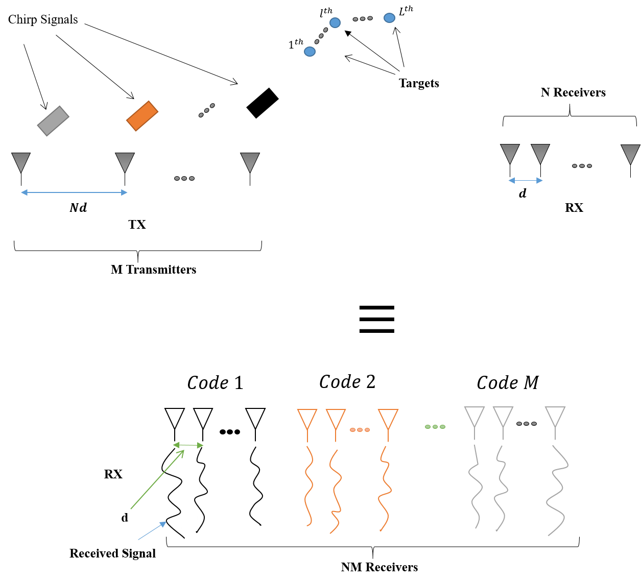
Figure 1: A schematic of a virtual MIMO radar based on CDM technique.

In the case of the CDM based MIMO radar each chirp is fired with a specific phase. In this paper we only consider two values for the phase, 0 and 180 degree. Upon applying orthogonal codes we can then create orthogonal signals in space. The up-chirp signal for the case of the CDM based virtual FMCW MIMO radar is given as

$$s^{(l)}_{mni}(t)=$$

$$\sigma_{l}\;e^{\displaystyle j2\pi f_{c}(t-\tau_{mnl})+j\pi\beta{(t-\tau_{mnl})}^{2}+j\varphi_{i}(m)}.$$ (2)

In (II), $\varphi_{i}(m)\in\{0,\pi\}$ where $i\in\{1,2,\cdots,N_{c}\}$ and $N_{c}$ is the code length. The dependency of $\varphi_{i}$ on $m$ is the indication of the fact that for each transmitter a unique code is used.

After the signal is received at the receiver it will be mixed with a copy of the transmitted signal and the result would be the beat signal. Based on (II) the beat signal for the signal transmitted by the $m^{\rm th}$ transmitter and received at the location of the $n^{\rm th}$ receiver is then expressed as,

$$s^{(l)}_{mni}(t)=$$

$$\sigma_{l}\;e^{\displaystyle-j2\pi f_{c}\tau_{mnl}-j2\pi\beta t\tau_{mnl}+j\pi\beta\tau_{mnl}^{2}+j\varphi_{i}(m)}.$$ (3)

Fig. 2 illustrates a schematic of our set-up. In Fig. 2 we have M transmit and N receive antennas. Parameters $r$ and $\theta$ are the range and incidence angle of a target in front of the array, respectively. Finally, $d_{r}$ is the element spacing between receive antennas and $d_{t}$ is the element spacing between transmit antennas.

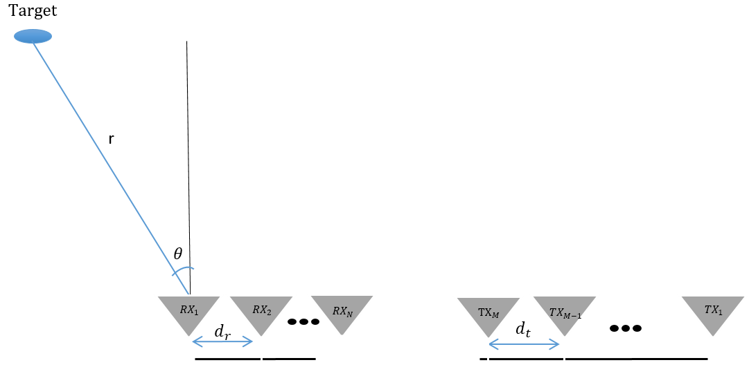
Figure 2: Set-up geometry for a MIMO array with M transmit and N receive antennas.

We place receiver number one at origin and it will be our reference point as has been shown in Fig. 2. Our processing will be based on this choice for the reference point. Based on this choice for the reference point the time delay $\tau_{mnl}$ can be written as $\tau_{mnl}=\frac{2}{c}(r_{l}+0.5d_{mn}sin(\theta_{l}))$, in which the $MN\times 1$ vector ${\bf d}$ is expressed as

$${\bf d} =\begin{pmatrix}\begin{bmatrix}(N-1)d_{r}\\ (N-2)d_{r}\\ \vdots\\ 0\\ \end{bmatrix}\bigotimes\begin{bmatrix}0\\ d_{t}\\ \vdots\\ (M-1)d_{t}\\ \end{bmatrix}\end{pmatrix},$$ (4)

where $\bigotimes$ stands for the Kronecker product. Since $r_{l}\ll c$, hence we ignore the last term in (II) and consider the beat signal as,

$$s^{(l)}_{mni}(t)=\sigma_{l}\;e^{\displaystyle-j2\pi f_{c}\tau_{mnl}-j2\pi\beta t\tau_{mnl}+j\varphi_{i}(m)}.$$ (5)

The next step is the decoding. To accomplish this goal the signal at the output of each receiver will be multiplied by a specific code that has already been used for each transmitter and the result is expressed as

$$\bar{{\bf s}}^{(l)}_{mn}=\sum\limits_{i=1}^{N_{c}}(\hat{{\bf s}}^{(l)}_{mni}\bigodot e^{j\varphi_{i}(m)}\b{1}_{1\times\tilde{N}}).$$ (6)

In (6), $\hat{{\bf s}}^{(l)}_{mni}=[s^{(l)}_{mni}(1),s^{(l)}_{mni}(2),\cdots,s^{(l)}_{mni}(\tilde{N})]$, where $\tilde{N}=T/t_{s}$, in which $t_{s}$ is the sampling time, and $\b{1}=[1,1,\cdots,1]_{(1\times\tilde{N})}$. The symbol $\bigodot$ stands for the Hadamard product. In the case of having $L$ targets in front of the radar the signal received by the radar is a linear combination of all these signals. Therefore, the signal received by the radar from all the signals $\bar{{\bf s}}^{(l)}_{mn}$, for $l\in\{1,2,\cdots,L\}$, can be described as

$$\tilde{\tilde{{\bf s}}}_{mn}=\sum\limits_{l=1}^{L}\bar{{\bf s}}^{(l)}_{mn}.$$ (7)

In the next section we address the calibration process.

III Calibration

Calibration plays an important role in radar imaging. In this section we present a very effective way to calibrate the FMCW MIMO radar. To calibrate the system, we use a target at a specific range and incidence angle which we refer to them as $r_{ref}\;\rm and\;\theta_{ref}$. We then multiply the signal received from targets with the reference signal and the result is given as

$$\underline{{\bf s}}_{mn}=\tilde{\tilde{{\bf s}}}_{mn}\bigodot\mathfrak{{\bar{s}}}^{*}_{mn},$$ (8)

where $\mathfrak{{\bar{s}}}^{*}_{mn}$ is a signal given as in (6) for a target located at $(r_{ref},\theta_{ref})$ and ^(∗) stands for the complex conjugate operator. The next step is to multiply (8) by the following term in order to restore the correct range of the targets

$$\tilde{{\bf s}}_{mn}=\underline{{\bf s}}_{mn}\bigodot\mathbf{\Im},$$ (9)

in which $\mathbf{\Im}=[1\;e^{j4\pi(f_{c}+(\frac{b}{\tilde{N}}))\frac{r_{ref}}{c}}\;\cdots\;e^{j4\pi(f_{c}+(\frac{b}{\tilde{N}})(\tilde{N}-1))\frac{r_{ref}}{c}}]$. In the next section we present image reconstruction technique to find the range and angle of arrival of targets.

IV Image Reconstruction

In this section we address an algorithm to reconstruct the range-angle information from the raw data. To set the stage we calculate the $MN\tilde{N}\times MN\tilde{N}$ sample covariance matrix as follows

$${\bf R}=\mathbb{E}\{\underline{{\bf s}}^{T}\underline{{\bf s}}\},$$ (10)

where $\underline{{\bf s}}=[\tilde{{\bf s}}_{11}\;\tilde{{\bf s}}_{12}\;\cdots\;\tilde{{\bf s}}_{1N}\;\tilde{{\bf s}}_{21}\;\cdots\;\tilde{{\bf s}}_{2N}\;\cdots\;\tilde{{\bf s}}_{MN}]$ and $\tilde{{\bf s}}_{mn}\;\rm for\;m\in\{1,2,\cdots,M\},\;n\in\{1,2,\cdots,N\}$ is given as in (9). In practice, however, we only have access to limited number of different realizations of ${\bf s}$. Therefore, we can only obtain an estimate of (10) which is called the sample covariance matrix. The steering vector is defined as

$${\bf a}(r,\theta)=e^{\displaystyle j2\pi\frac{2}{c}(r+0.5{\bf d}sin(\theta))\bigotimes{\bf g}},$$ (11)

where ${\bf g}=[f_{c}\;f_{c}+\frac{b}{\tilde{N}}\;\cdots\;f_{c}+\frac{b}{\tilde{N}}(\tilde{N}-1)]^{T}$. Consequently, the image provided by the MUSIC algorithm for a target located at $r$ with angle of arrival $\theta$ is expressed as

$$\mathcal{I}_{\rm{MUSIC}}(r,\theta)={\frac{{{{\bf a}^{\dagger}(r,\theta)}{\bf a}(r,\theta)}}{{{\bf a}^{\dagger}(r,\theta)}{{\bf E}}{{\bf E}^{\dagger}}{\bf a}(r,\theta)}},$$ (12)

where ${{\bf a}}(r,\theta)$ is the steering vector given in (11) and the columns of ${{\bf E}}\in\mathbb{C}^{MN\tilde{N}\times(MN\tilde{N}-L)}$ are the eigenvectors of the sample covariance matrix corresponding to the smallest $MN\tilde{N}-L$ eigenvalues with $L$ being the effective dimension of the signal subspace. Finally, ^(†) stands for the complex conjugate transpose operator.

V Experimental Results

In this section we present the experimental results. We have used a FMCW radar operating at 79GHz with 3 transmitters and 4 receivers. The radar chip along with its transmit and receive antennas has been shown in Fig. 4. The bandwidth and length of the transmitted up-chirp are $1.5GHz$ and $25.6\mu s$, respectively. The output power is $5dBm$. The gain for both transmit and receive antennas is $14dB$ at boresight. The sampling frequency of the ADC is $20MHz$. We have set the maximum range at 3m and based on the values given for the bandwidth and the chirp time, the beat frequency for a target at $R=3m$ is $f_{b}=\frac{b}{T}\frac{2R}{c}=1.17MHz$. Therefore, we have downsampled the signals by factor $8$.

From Fig. 4, we see that $d_{r}=\frac{\lambda}{2}$ and $d_{r}=2\lambda$ and as a result $d_{t}=4d_{r}$ which is an indication that virtual MIMO processing is possible and we can effectively increase the number of receive elements from 4 to $3\times 4$.

To implement the idea of CDM based virtual FMCW MIMO radar we have used Walsh code [10] of length 8. We utilize the following three codes for the three transmitters
$TX1=[+1\;+1\;+1\;+1\;-1\;-1\;-1\;-1]$,
$TX2=[+1\;+1\;-1\;-1\;+1\;+1\;-1\;-1]$,
$TX3=[+1\;-1\;+1\;-1\;+1\;-1\;+1\;-1]$,
where +1 and -1 represent 0 and 180 degree phase shift, respectively,

Fig. 3 shows the flow chart of the proposed algorithm for our CDM based virtual FMCW MIMO radar. The purpose of the Hilbert transform [11] block is to transform the output data of the ADC from real numbers to complex numbers and prepare the data for calibration.

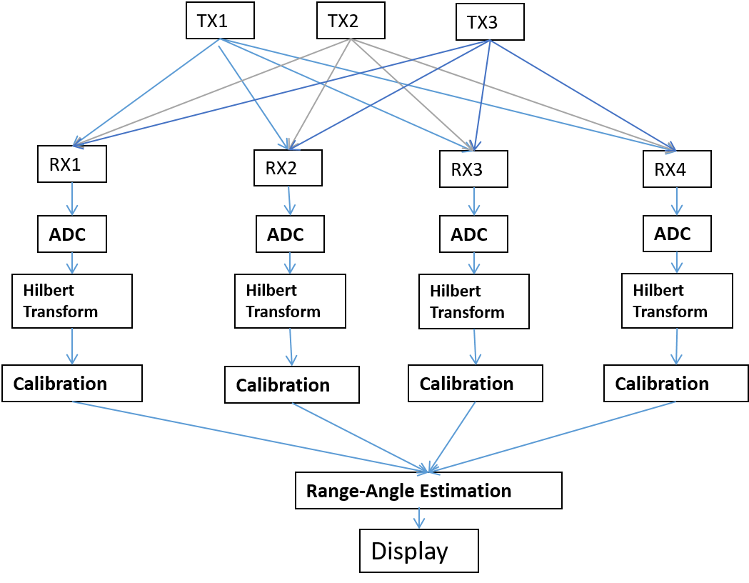
Figure 3: The flow chart of the algorithm.

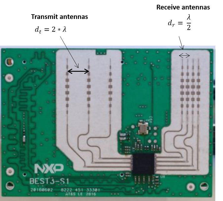
Figure 4: The radar chip with its transmit and receive antennas.

Fig. 5 shows the experimental set-up where there are two $20dBsm$ reflectors in front of the radar at $(195cm,19^{\circ})$, $(214cm,-29^{\circ})$.

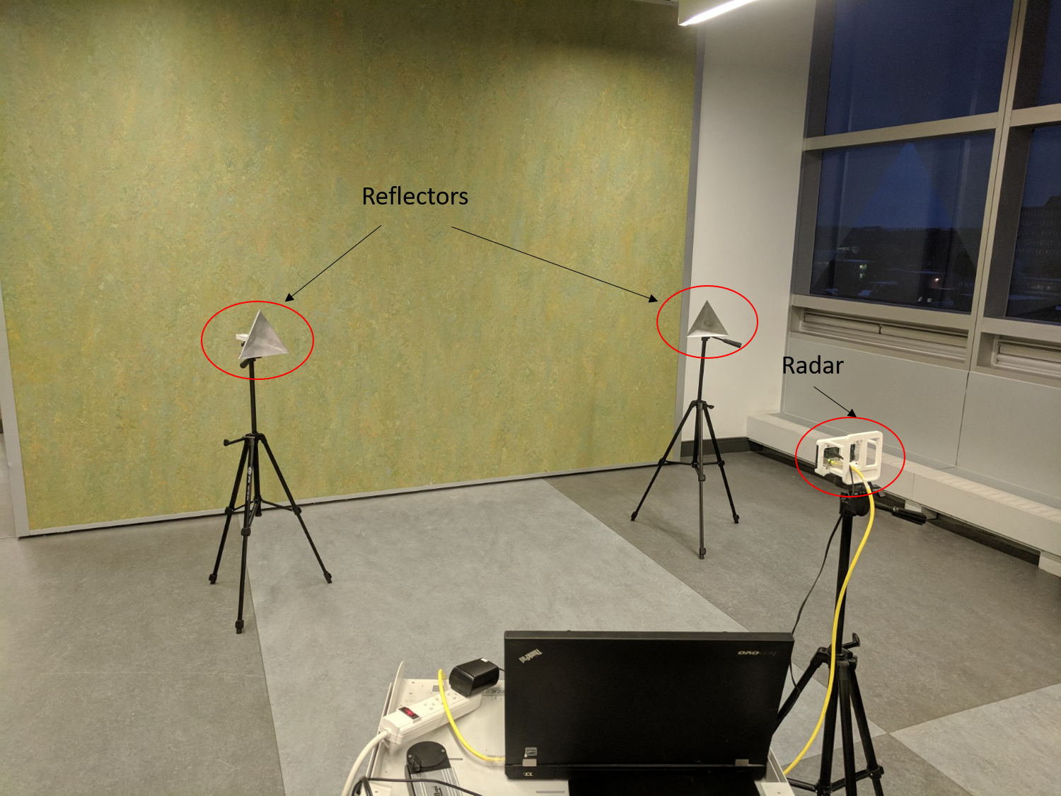
Figure 5: The experimental set-up for two 20dBsm reflectors in front of the radar.

Fig. 6 illustrates the result of applying (12) to the experimental data. The dimension for the signal subspace has been set to 2. We have used 42 different realizations of the received signal to calculate an estimate of the covariance matrix given in (10).

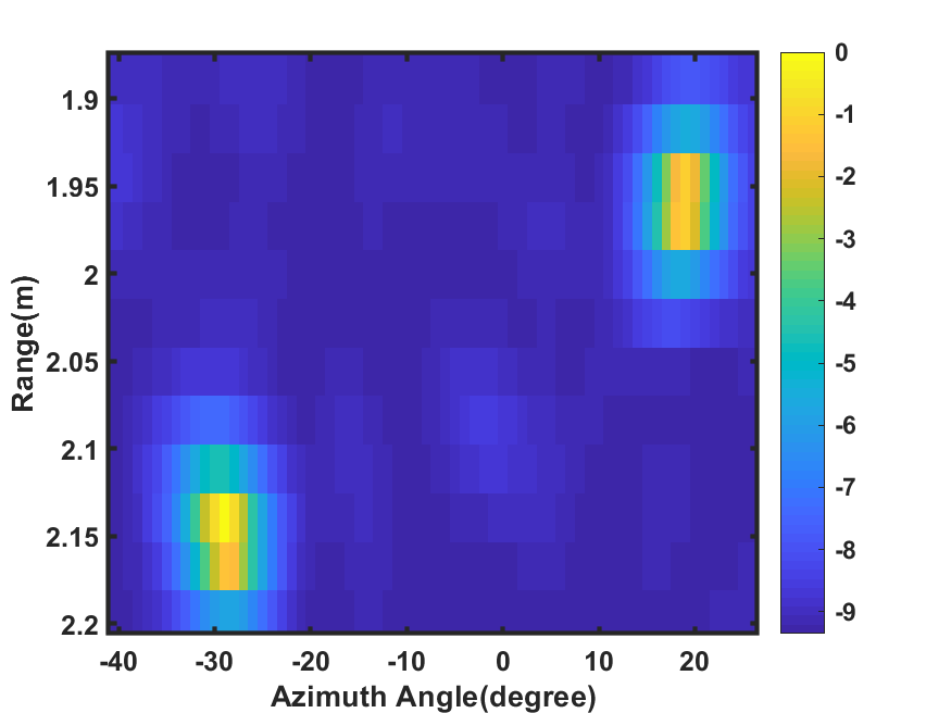
Figure 6: The result of applying (12) to the experimental data gathered from the set-up shown in Fig.  5.

VI Conclusion

In this paper we presented a full description of 2D radar imaging for a CDM based virtual FMCW MIMO radar. We started with the problem formulation and then addressed the system calibration at the baseband level. Based on the presented model we described a 2D MUSIC algorithm for image reconstruction. Finally we have shown the result of applying the MUSIC technique to the data gathered from a CDM based virtual FMCW MIMO radar operating at 79GHz with 3 transmitters and 4 receivers using Walsh code of length 8.

VII Acknowledgement

The authors would like to thank NSERC, NXP Semiconductors and MAGNA for their supports.

References

- [1] S. Hamidi, M. Nezhad-Ahmadi, and S. Safavi-Naeini, “TDM based virtual FMCW MIMO radar imaging at 79GHz,” pp. 1–2, 2018.
- [2] M. Harter, T. Schipper, L. Zwirello, A. Ziroff, and T. Zwick, “24GHz digital beamforming radar with t-shaped antenna array for three-dimensional object detection,” International Journal of Microwave and Wireless Technologies, vol. 4, no. 3, 2012.
- [3] R. Feger, C. Pfeffer, C. M. Schmid, M. J. Lang, Z. Tong, and A. Stelzer, “A 77-GHz FMCW MIMO radar based on loosely coupled stations,” pp. 1–4, Mar. 2012.
- [4] H. W. Tao Chen and L. Liu, “A joint doppler frequency shift and DOA estimation algorithm based on sparse representations for colocated TDM-MIMO radar,” Journal of Applied Mathematics, 2014.
- [5] J. Guetlein, A. Kirschner, and J. Detlefsen, “Calibration strategy for a TDM FMCW MIMO radar system,” pp. 1–5, Oct. 2013.
- [6] C. M. Schmid, R. Feger, C. Pfeffer, and A. Stelzer, “Motion compensation and efficient array design for TDMA FMCW MIMO radar systems,” pp. 1746–1750, Mar. 2012.
- [7] M. K. A. Zwanetski and H. Rohling, “Waveform design for FMCW MIMO radar based on frequency division,” IRS 2013, 14th International Radar Symposium, Dresden, DE, pp. 19–21, Jun. 2013.
- [8] R. Schmidt, “Multiple emitter location and signal parameter estimation,” IEEE Transactions on Antennas and Propagation, vol. 34, no. 3, pp. 276–280, 1986.
- [9] P. Stoica and N. Arye, “MUSIC, maximum likelihood, and Cramer-Rao bound,” IEEE Transactions on Acoustics, Speech and Signal Processing, vol. 37, no. 5, pp. 720–741, 1989.
- [10] K.Usha1 and K. J. Sankar, “Generation of Walsh codes in two different orderings using 4-bit Gray and Inverse Gray codes,” Indian Journal of Science and Technology, vol. 5, no. 3, Mar. 2012.
- [11] S. L. Hahn, Hilbert Transforms in Signal Processing. Artech House, Inc., 1996.