Energy Reflection and Transmission at 2D Holographic Interfaces

Abstract

Scattering from conformal interfaces in two dimensions is universal in that the flux of reflected and transmitted energy does not depend on the details of the initial state. In this letter, we present the first gravitational calculation of energy reflection and transmission coefficients for interfaces with thin-brane holographic duals. Our result for the reflection coefficient depends monotonically on the tension of the dual string anchored at the interface, and obeys the lower bound recently derived from the ANEC in conformal field theory. The B(oundary)CFT limit is recovered for infinite ratio of the central charges.

1. Introduction.– Conformal interfaces are ubiquitous both in condensed-matter systems and in studies of the holographic duality. Such interfaces describe the local, scale-invariant gluing of two conformal field theories, CFT_L on the left and CFT_R on the right. Examples include junctions of quantum wires Wong and Affleck (1994), line or surface defects in the critical 2D or 3D Ising models Oshikawa and Affleck (1997), or the gluing of superconformal gauge theories with different couplings and/or gauge groups. In bottom-up AdS/CFT, interfaces are often modeled by codimension-one branes anchored at the AdS boundary. Smooth (super)gravity solutions describing top-down embeddings in string theory are also known. Some early papers on the subject are Karch and Randall (2001a, b); Porrati (2002); DeWolfe et al. (2002); Bachas et al. (2002); Bak et al. (2003). Additional references will be given as we proceed.

Folding spacetime along an interface converts the latter to a conformal boundary of the product theory CFT${}_{L}\otimes\overline{\rm CFT}_{R}$, where the bar indicates space reflection. The folded theory has two energy-momentum tensors, $T_{L}$ and $\bar{T}_{R}$, that are separately conserved in the bulk while only their sum, $T_{\rm tot}\equiv T_{L}+\bar{T}_{R}$, needs to be conserved at the boundary. What distinguishes interfaces from boundaries (and ICFTs from BCFTs) is the existence of another, relative spin-2 current $T_{\rm rel}=c_{R}T_{L}-c_{L}\bar{T}_{R}$ , which measures the exchange of energy between left and right. Here $c_{L}$ and $c_{R}$ are the central charges of the two CFTs. As usual, things simplify considerably in two dimensions. In this case, it was noted in Quella et al. (2007) and further analyzed in Kimura and Murata (2015); Billó et al. (2016); Meineri et al. (2020) that the transfer of energy across the interface is controlled by a single transmission or reflection coefficient, ${\cal T}$ or ${\cal R}$, with ${\cal T}+{\cal R}=1$. The purpose of the present note is to derive a formula for these coefficients in the simplest holographic-interface model.

The model consists of two AdS₃ slices separated by a string of tension $\sigma$. The AdS₃ slices have radii $\ell_{L}$ and $\ell_{R}$, related to the CFT central charges by the Brown-Henneaux formula $c_{L,R}=3\ell_{L,R}/2G$ Brown and Henneaux (1986), where $G$ is the three-dimensional Newton’s constant. With no loss of generality we take $\ell_{L}\geq\ell_{R}$, so that the ‘false’ higher-energy AdS vacuum is on the left, while the ‘true’ AdS vacuum is on the right. For tensions inside the interval

$$0\leq{1\over\ell_{R}}-{1\over\ell_{L}}\,\leq\,8\pi G\sigma\,\leq\,{1\over\ell_{R}}+{1\over\ell_{L}}$$ (1)

the string-worldsheet geometry is AdS₂ corresponding to the ground state of the ICFT Karch and Randall (2001b); Bachas (2003). At the extremal values of the interval the worldsheet flattens out, i.e., the AdS₂ radius diverges. The lower $\sigma$ limit in (1) actually corresponds to the Coleman-De Lucia bound Coleman and De Luccia (1980) below which the false AdS₃ vacuum is unstable to nucleation of bubbles. This is also the BPS bound for supergravity domain walls Cvetic et al. (1992). The upper limit, on the other hand, corresponds to the Randall-Sundrum fine-tuned tension, beyond which the string worldsheet becomes de Sitter and gets anchored on a spacelike curve of the conformal boundary Karch and Randall (2001b).

This model has been used as a toy model of holographic defects, in particular for calculations of holographic entanglement entropy, see e.g., Azeyanagi et al. (2008). In this letter we provide the first calculation of its transport properties. Our main result is the following formula for the energy-transmission coefficient defined in Quella et al. (2007),

$${\cal T}={4\over\ell_{L}+\ell_{R}}\left[{1\over\ell_{L}}+{1\over\ell_{R}}+8\pi G\sigma\right]^{-1}\ .$$ (2)

Together with the central charges, ${\cal T}$ was shown Quella et al. (2007) to parametrize the most general two-point functions of energy-momentum tensors allowed by the symmetries of the problem.

As explained in Kimura and Murata (2015); Meineri et al. (2020), what was actually defined in Quella et al. (2007) is the weighted-average transmission coefficient

$$\hskip-14.22636pt{\cal T}={c_{L}{\cal T}_{L}+c_{R}{\cal T}_{R}\over c_{L}+c_{R}}\,,\ \ {\rm where}\ \ {\cal T}_{L,R}={(c_{L}+c_{R}){\cal T}\over 2c_{L,R}}$$ (3)

are the transmission coefficients for excitations incident on the interface from the left and right, respectively. Our formula for these directional transmission coefficients reads

$${\cal T}_{L,R}={2\over\ell_{L,R}}\left[{1\over\ell_{L}}+{1\over\ell_{R}}+8\pi G\sigma\right]^{-1}\ .$$ (4)

The calculation of (2) and (4) is performed by scattering surface-gravity waves in a semiclassical geometry dual to the ground state of the ICFT. It relies on the usual condition of no outgoing waves at the Poincaré horizon, whose subtle implementation we explain below.

Before describing the calculation in detail, let us comment on some salient features of our result. First, both ${\cal T}_{L}$ and ${\cal T}_{R}$ are monotonically-decreasing functions of the tension $\sigma$. Their maximal and minimal values (in terms of the central charges) read

$$\begin{split}\,\hskip-14.22636pt{\cal T}_{L,R}^{\rm max}={c_{R}\over c_{L,R}}\ \ ,\qquad{\cal T}_{L,R}^{\rm min}={c_{R,L}\over c_{L}+c_{R}}\ ,\end{split}$$ (5)

or equivalently for the average coefficients

$$\begin{split}{2c_{L}c_{R}\over(c_{L}+c_{R})^{2}}\,\leq\,{\cal T}\leq{2c_{R}\over c_{L}+c_{R}}\ \ \ \Longleftrightarrow\\ \ \ \ {c_{L}^{2}+c_{R}^{2}\over(c_{L}+c_{R})^{2}}\,\geq\,{\cal R}\geq{c_{L}-c_{R}\over c_{L}+c_{R}}\ .\end{split}$$ (6)

The above lower bound on ${\cal R}$ is the same as the one following from the achronal average-null-energy condition (AANEC) in the ICFT Meineri et al. (2020). As stressed in that reference, this lower bound is stronger than the bound imposed by reflection positivity of the Euclidean theory Billó et al. (2016), ${\cal R}\geq({c_{L}-c_{R}\over c_{L}+c_{R}})^{2}$. This shows that reflection positivity does not necessarily imply the ANEC in ICFTs.

If the inequality $c_{L}>c_{R}$ is strict, both ${\cal T}_{L}$ and ${\cal T}$ are less than 1. Total transmission to signals incident from both sides is therefore only possible between degenerate AdS₃ vacua separated by a tensionless string. This is the gravitational counterpart of a topological interface.

The opposite limit of total reflection, ${\cal R}\to 1$, can only be reached by taking $c_{R}/c_{L}\to 0$, i.e., by depleting CFT_R of degrees of freedom, relative to CFT_L. This should be contrasted with the fact that in more general ICFTs, factorizable interfaces can impose reflecting boundary conditions on each side for any values of $c_{L}$, $c_{R}$. In our minimal holographic model, on the other hand, the transmission of energy incident from the left can be shut down only if there are no degrees of freedom in the right side. Note however that in this limit ${\cal T}_{R}=1$, so that the (scarce) signals incident from the right are fully transmitted to the other side.

We should here stress that the transport coefficient ${\cal T}$ (or ${\cal R}$) and the ground-state entropy (the logarithm of the $g$-factor) Affleck and Ludwig (1991) are independent properties of an interface. This is illustrated by topological interfaces in free-field models which can have arbitrarily large entropy Fuchs et al. (2007); Bachas and Brunner (2008) even though their transmission coefficient is always ${\cal T}=1$. The holographic duals of such interfaces are tensionless branes Fliss et al. (2017); Gutperle and Miller (2019), so tension is not necessarily tied to entropy. Entanglement entropy, which contains the ground-state entropy as a finite correction to the leading logarithmically divergent term, has been computed in a variety of holographic ICFT models, e.g., Azeyanagi et al. (2008); Chiodaroli et al. (2010); Jensen and O’Bannon (2013); Erdmenger et al. (2015); Gutperle and Miller (2016). It would be interesting to calculate transport coefficients in these models to see how, if at all, they are correlated with entropy.

2. Holographic scattering states.– We describe now the main steps in the calculation of the reflection and transmission coefficients. As mentioned above, we use a minimal holographic model for the ICFT, consisting of two manifolds $M_{L,R}$ that are locally AdS₃ and are joined on the worldsheet of a tensile string. The asymptotic boundaries of these manifolds are the left, respectively right half-planes glued along the CFT interface $P$. The latter extends in the bulk to surfaces $Q_{L}\subset M_{L}$ and $Q_{R}\subset M_{R}$ that are identified with each other and with the worldsheet of the string, see figure 1. The gluing of $M_{L}$ to $M_{R}$ must obey the matching conditions Israel (1966)

$$\gamma_{L,\alpha\beta}= \gamma_{R,\alpha\beta}\,,$$ (7a)

$$[K_{\alpha\beta}]-[\textrm{tr}K]\gamma_{\alpha\beta}= 8\pi G\sigma\,\gamma_{\alpha\beta}\,,$$ (7b)

where we have denoted by $\gamma_{L,R}$ and $K_{L,R}$ the induced metric and extrinsic curvature on $Q_{L,R}$, respectively, and we use $[X]\equiv X_{L}-X_{R}$ to indicate discontinuities on the two sides of the interface.

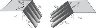
Figure 1: Illustration of the holographic-interface geometry. The two spacetimes are glued together at the location of the worldsheet $Q_{L}\equiv Q_{R}$. The interface $P$ is the intersection of the worldsheet with the conformal boundary. The incident wave is denoted by $I$, and the reflected and transmitted waves are denoted by $R$ and $T$.

The ICFT vacuum is described in Fefferman-Graham coordinates by the solution Karch and Randall (2001b); Bachas (2003)

$$\hskip-5.69054ptds^{2}_{L}=\frac{\ell_{L}^{2}}{y_{L}^{2}}[dy_{L}^{2}+du_{L}^{2}-dt_{L}^{2}]\ \ \ {\rm for}\,\ u_{L}\leq y_{L}\tan\theta_{L},$$ (8)

$$\hskip-5.69054ptds^{2}_{R}=\frac{\ell_{R}^{2}}{y_{R}^{2}}[dy_{R}^{2}+du_{R}^{2}-dt_{R}^{2}]\,\ \ {\rm for}\,\ u_{R}\geq-y_{R}\tan\theta_{R},$$

where $0\leq y_{L,R}<\infty$. The worldsheet $u_{L}=y_{L}\tan\theta_{L}$ or $u_{R}=-y_{R}\tan\theta_{R}$ subtends an angle ${\pi\over 2}+\theta_{L}$, respectively ${\pi\over 2}+\theta_{R}$, to the left/right halves of the conformal boundary. The worldsheet metric is AdS₂ with radius $\ell_{W}$ obeying

$$\ell_{W}={\ell_{L}\over\cos\theta_{L}}={\ell_{R}\over\cos\theta_{R}}={\tan\theta_{L}+\tan\theta_{R}\over 8\pi G\sigma}\,.$$ (9)

The first two equalities follow from (7a) and the last one from (7b). It will be later convenient to employ the rotated coordinates

$$\begin{split}\begin{pmatrix}u_{L}\\ y_{L}\end{pmatrix}&=\begin{pmatrix}\cos\theta_{L}&\sin\theta_{L}\\ -\sin\theta_{L}&\cos\theta_{L}\end{pmatrix}\begin{pmatrix}x_{L}\\ z_{L}\end{pmatrix}\,,\ \ \ \,\\ \begin{pmatrix}u_{R}\\ y_{R}\end{pmatrix}&=\begin{pmatrix}\cos\theta_{R}&-\sin\theta_{R}\\ \sin\theta_{R}&\cos\theta_{R}\end{pmatrix}\begin{pmatrix}x_{R}\\ z_{R}\end{pmatrix}\ ,\end{split}$$ (10)

in which the unperturbed string sits at $x_{L}=x_{R}=0$, and its worldsheet can be parametrized by $t_{L}=t_{R}\equiv t$ and $z_{L}=z_{R}\equiv z$.

In principle one would like to solve the matching problem (7) for a generic metric and a fluctuating interface on the conformal boundary. It is however sufficient for our purposes here to set all ICFT sources to zero, and only consider normalizable excitations of the fields. These are particularly simple in pure AdS₃ where the most general solution of the Einstein equations in Fefferman-Graham coordinates can be written as Skenderis and Solodukhin (2000) (see also Banados (1999); Balasubramanian et al. (1999); Rooman and Spindel (2001); Krasnov (2003))

$$ds^{2}=\frac{\ell^{2}dy^{2}}{y^{2}}+\Bigl{[}\frac{\ell^{2}g^{(0)}_{\alpha\beta}}{y^{2}}+g^{(2)}_{\alpha\beta}+{y^{2}\over 4\,\ell^{2}}g^{(4)}_{\alpha\beta}\Bigr{]}dw^{\alpha}dw^{\beta}$$ (11)

with $g^{(4)}=g^{(2)}(g^{(0)})^{-1}g^{(2)}$ and, for flat boundary metric, $g^{(2)}_{\alpha\beta}=4G\ell\langle T_{\alpha\beta}\rangle$. Here $\langle T_{\alpha\beta}\rangle$ is the vev of the canonically-normalized, traceless conserved energy-momentum tensor in some state of the dual CFT. Linearizing in the perturbation allows us to drop $g^{(4)}$, so that the correction to the standard AdS₃ Poincaré metric has arbitrary left- and right-moving waves, $g^{(2)}_{++}(w^{+})$ and $g^{(2)}_{--}(w^{-})$.

In order to reproduce the setup of ref. Meineri et al. (2020) we consider a configuration with an incoming wave from the left, giving rise to a reflected wave on the left and a transmitted wave on the right. Explicitly, identifying the $w^{\pm}$ of (11) with $u\pm t$, and using monochromatic waves, we have

$${\bigl{[}ds^{2}\bigr{]}^{(2)}_{L}}= 4G\ell_{L}\epsilon\Bigl{[}e^{i\omega(t_{L}-u_{L})}\,d(t_{L}-u_{L})^{2}+$$ (12)

$$\hskip 34.1433pt{\cal R}_{L}\,e^{i\omega(t_{L}+u_{L})}\,d(t_{L}+u_{L})^{2}\Bigr{]}+c.c.\ ,$$

$${\bigl{[}ds^{2}\bigr{]}^{(2)}_{R}}= 4G\ell_{R}\epsilon\,{\cal T}_{L}e^{i\omega(t_{R}-u_{R})}\,d(t_{R}-u_{R})^{2}+c.c.\,,$$

where ${\cal R}_{L}$ and ${\cal T}_{L}$ are the (a priori complex) relative amplitudes of the reflected and transmitted waves, and the subscript $L$ indicates that the incident wave came from the left. Anticipating the final result, we give the same names to these amplitudes as to the (real) reflection and transmission coefficients. In what follows, we will linearize our equations in the incoming flux $|\langle T_{--}\rangle|=\epsilon$.

Gluing $M_{L}$ with $M_{R}$ requires matching coordinates on the worldsheet. We allow for this by writing $z_{L,R}=z+{\tilde{\epsilon}}\,\zeta_{L,R}(z,t)$ and $t_{L,R}=t+\tilde{\epsilon}\,\lambda_{L,R}(z,t)$, where $z,t$ are the Poincaré coordinates of the AdS₂ worldsheet and we defined for convenience $\tilde{\epsilon}={4G\over\ell_{W}}\,\epsilon$. Since we are keeping only linear order in $\epsilon$, we can set $t_{L}=t_{R}=t$ and $z_{L}=z_{R}=z$ in the perturbation (12). The above changes of coordinates enter only through the expansion of the leading worldsheet metric and extrinsic curvatures in (7). We also let $x_{L,R}=\tilde{\epsilon}\,\delta_{L,R}(z,t)$ be the fluctuating position of the string in the transverse dimension.

Thanks to time-translation invariance we are allowed to work at fixed frequency,

$$\delta_{L,R}(z,t)=e^{i\omega t}\delta_{L,R}(z)+c.c.$$ (13)

and similarly for $\zeta_{L,R}$ and $\lambda_{L,R}$.

We have then six equations for the six functions $\delta_{L,R}$, $\zeta_{L,R}$ and $\lambda_{L,R}$. But common reparametrizations of the two charts are pure gauge, so only the transition functions

$$\zeta\equiv\zeta_{L}-\zeta_{R}\quad{\rm and}\quad\lambda\equiv\lambda_{L}-\lambda_{R}$$ (14)

enter in the equations (7). The problem may now look overconstrained, but two of the matching conditions (7b) are not actually independent equations. The reason is that all foliations of AdS₃ obey the momentum constraints

$$D^{\alpha}K_{\alpha\beta}-D_{\beta}K=0\ ,$$ (15)

where $D_{\alpha}$ is the covariant derivative with respect to the induced metric. Thus, once one of the equations (7b) has been solved, the other two are automatically satisfied up to constants.

The brane fluctuations are induced by the gravity waves (12). The equations are more compact in terms of the combinations

$$\hskip-11.38109ptD\equiv\delta_{L}-\delta_{R}\,,\ \ \ \Delta\equiv\tan\theta_{L}\delta_{L}+\tan\theta_{R}\delta_{R}-\zeta\,.$$ (16)

The four independent matching conditions read

$$\Delta{\,+\,i\omega z\lambda}\,=\,z^{3}\Bigl{[}{\cos\theta_{L}\over 2}({\bf I}+{\bf R})-{\cos\theta_{R}\over 2}{\bf T}\Bigr{]}\,,$$ (17)

$$i\omega z\zeta{\,-\,z\partial_{z}\lambda}\ \,=\,z^{3}\Bigl{[}{\sin\theta_{R}}\cos\theta_{R}{\bf T}+{\sin\theta_{L}}\cos\theta_{L}({\bf I}-{\bf R})\Bigr{]}\,,$$

$$z\partial_{z}\zeta+\Delta\,=\,z^{3}\Bigl{[}{\sin^{2}\theta_{R}\cos\theta_{R}\over 2}{\bf T}-{\sin^{2}\theta_{L}\cos\theta_{L}\over 2}({\bf I}+{\bf R})\Bigr{]}\,,$$

$$z\partial_{z}D=z^{3}\Bigl{[}{1\over i\omega z}({\bf I}-{\bf R}-{\bf T})-{\sin\theta_{L}\cos^{2}\theta_{L}\over 2}({\bf I}+{\bf R})$$

$$\hskip 85.35826pt-{\sin\theta_{R}\cos^{2}\theta_{R}\over 2}{\bf T}\Bigr{]}\ ,$$

where

$$\begin{split}&{\bf I}\equiv e^{-i\omega\sin\theta_{L}z},\ {\bf R}={\cal R}_{L}\,e^{i\omega\sin\theta_{L}z},\ \\ &~{}~{}~{}~{}~{}~{}~{}~{}~{}~{}~{}~{}~{}{\bf T}\equiv{\cal T}_{L}e^{i\omega\sin\theta_{R}z}\end{split}$$ (18)

are the exponentials imprinted on the worldsheet by the graviton waves (12). The first three equations are the matching conditions (7a) while the fourth is the $(tz)$ component of (7b), where we have used the second equation to simplify it. The three (almost) redundant matching conditions can be actually combined into an algebraic equation for $D$, so the integration constant in the last equation of (17) is fixed as in eq. (20), see below.

Consider first the homogeneous equations obtained by setting the right-hand sides in (17) to zero. The general solution reads

$$-i\omega\lambda(z)={\Delta(z)\over z}={a_{+}}e^{i\omega z}+{a_{-}}e^{-i\omega z}\,,$$

$$-i\omega\zeta(z)={a_{+}}e^{i\omega z}-{a_{-}}e^{-i\omega z}\,,\quad D=0\ .$$ (19)

The $z=0$ limit of these functions corresponds to sources in the dual ICFT. For instance $\delta_{L}(0)=\delta_{R}(0)$ is a source for the interface displacement operator. Linearizing in this source gives an $O(z^{-3})$ correction to the induced metric. This is consistent with the fact that the scaling dimension of the displacement operator is $\mathfrak{D}=2$ Billó et al. (2016). In the absence of gravity waves, setting the sources to zero implies $a_{+}=a_{-}=0$. This shows that there are no normalizable states supported entirely by the interface.

Let’s go back now to the inhomogeneous equations (17). Since these are linear equations, the general solution is given by (Energy Reflection and Transmission at 2D Holographic Interfaces) plus some special solution. The result after straightforward manipulations is

$$\begin{split}\frac{\Delta(z)}{z}=&\frac{1}{\omega^{2}\cos\theta_{L}}\left({\bf I}+{\bf R}\right)-\frac{1}{\omega^{2}\cos\theta_{R}}{\bf T}+a_{+}e^{i\omega z}+a_{-}e^{-i\omega z}\,,\\ \zeta(z)=&-\frac{\cos\theta_{L}z}{\omega^{2}}\left({\bf I}+{\bf R}\right)-\frac{i}{\omega^{3}}\left({\bf I}-{\bf R}\right)\left(\tan\theta_{L}+\frac{\sin\theta_{L}\cos\theta_{L}}{2}\omega^{2}z^{2}\right)\\ &-\frac{i}{\omega^{3}}{\bf T}\left(\tan\theta_{R}+i\cos\theta_{R}\omega z+\frac{\sin\theta_{R}\cos\theta_{R}}{2}\omega^{2}z^{2}\right)+\frac{i}{\omega}\left(a_{+}e^{i\omega z}-a_{-}e^{-i\omega z}\right)\,,\\ \lambda(z)=&\frac{i}{\cos\theta_{L}\omega^{3}}\left({\bf I}+{\bf R}\right)\left(1-\frac{\cos^{2}\theta_{L}}{2}\omega^{2}z^{2}\right)-\frac{i}{\cos\theta_{R}\omega^{3}}{\bf T}\left(1-\frac{\cos^{2}\theta_{R}}{2}\omega^{2}z^{2}\right)+\frac{i}{\omega}\left(a_{+}e^{i\omega z}+a_{-}e^{-i\omega z}\right)\,,\\ D(z)=&-\frac{i}{\omega^{3}}\left({\bf I}-{\bf R}\right)\left(1+\frac{\cos^{2}\theta_{L}}{2}\omega^{2}z^{2}\right)+\frac{\sin\theta_{L}z}{\omega^{2}}\left({\bf I}+{\bf R}\right)+\frac{i}{\omega^{3}}{\bf T}\left(1-i\sin\theta_{R}\omega z+\frac{\cos^{2}\theta_{R}}{2}\omega^{2}z^{2}\right)\,.\end{split}$$ (20)

Requiring that the sources vanish now gives

$$D(0)=0\,\Longrightarrow\,{\cal R}_{L}+{\cal T}_{L}=1\ ,$$ (21)

and further from $\zeta(0)=\lambda(0)=0$ we obtain:

$$\hskip-25.60747pta_{+}={1\over 2\omega^{2}}\Bigl{[}{\cal T}_{L}\Bigl{(}\frac{1+\sin\theta_{R}}{\cos\theta_{R}}+\tan\theta_{L}\Bigr{)}-\frac{(1+{\cal R}_{L})}{\cos\theta_{L}}\Bigr{]}\,,$$ (22)

$$\hskip-25.60747pta_{-}={1\over 2\omega^{2}}\Bigl{[}{\cal T}_{L}\Bigl{(}\frac{1-\sin\theta_{R}}{\cos\theta_{R}}-\tan\theta_{L}\Bigr{)}-\frac{(1+{\cal R}_{L})}{\cos\theta_{L}}\Bigr{]}\,.$$ (23)

The reader can verify that with these choices all four functions are $O(z^{3})$ near the conformal boundary, and make $O(1)$ contributions to the worldsheet metric which can be interpreted as ICFT vevs. This agrees again with the fact that the scaling dimension of the displacement operator is two Billó et al. (2016).

Inserting the solution for $\delta_{L,R}$ in the expression for the induced metric shows that the latter is locally AdS₂ (constant intrinsic Ricci curvature). Thus, as is the case for homogeneous AdS₃/CFT₂, here too the dynamics happens at the conformal boundary in spite of the presence of the string/interface.

Up to this point, we have obtained a solution for the equations of motion of our model, that is valid for any value of ${\cal T}_{L}$. To proceed further, we have to make an assumption about the behaviour of the solution at the Poincaré horizon, as mentioned in the introduction. It is well-known that in the Lorentzian AdS/CFT correspondence the boundary conditions at the conformal boundary do not determine the solution uniquely, because there are normalizable modes that vanish at the boundary and are regular in the interior Balasubramanian et al. (1999); this is the dual of the property that there are different Minkowskian QFT propagators, depending on the choice of the initial state (retarded, advanced, Feynman etc.).

The prescription of Son and Starinets (2002); Herzog and Son (2003) (generalized by Skenderis and van Rees (2009)), frequently used in the literature, requires the absence of modes coming out of the horizon for the computation of a retarded correlator. In our case it is not immediately obvious how to apply this prescription, since the problem is not formulated as the computation of a causal response. One difficulty is that wave packets formed from (12) are localized in $u_{L,R}$ but not in the radial AdS coordinates $y_{L,R}$. Such wavepackets imprint superluminal waves on the functions $\delta_{L,R}$, $\zeta$ and $\lambda$ of the form $e^{i\omega t}\times({\bf I},{\bf R}\ {\rm or}\ {\bf T})$, see eq. (18). But as illustrated by seawaves hitting an oblique seashore, these superluminal waves carry no energy. To see why, one must look at gauge-invariant quantities left unchanged by common reparametrizations of the two charts, $\delta\zeta_{L}=\delta\zeta_{R}$ and $\delta\lambda_{L}=\delta\lambda_{R}$. One such quantity, at the linearized order considered here, is the traceless part of the extrinsic curvature which is continuous across the worldsheet by Israel’s matching condition (7b). A simple calculation gives

$$\hat{K}_{\pm\pm}=\frac{a_{\pm}\,\omega^{2}\epsilon}{2\pi\sigma\ell_{W}}e^{i\omega x^{\pm}}+\mathcal{O}(\epsilon^{2})\ ,$$ (24)

where $x^{\pm}=t\pm z$ and $\hat{K}_{\alpha\beta}$ denotes the traceless part of $K_{\alpha\beta}$. Note that the superluminal waves disappeared from the above expression, and that the ‘no outgoing wave’ condition reduces to $a_{+}=0$. Note in addition that the (discontinuous) trace parts, $K_{L,R}=\pm{2\over\ell_{W}}\tan(\theta_{L,R})+\mathcal{O}(\epsilon^{2})$, are not perturbed at linear order.

With the help of equations (21) and (22), the no-outgoing-wave condition implies

$${\cal T}_{L}=\frac{2\cos\theta_{R}}{\cos\theta_{R}(1+\sin\theta_{L})+\cos\theta_{L}(1+\sin\theta_{R})}\,.$$ (25)

Trading the angles for $\ell_{L,R}$ and $\sigma$ gives our result (4). It is non-trivial that ${\cal R}_{L}$ and ${\cal T}_{L}$, which started out as complex amplitudes in the gravitational-scattering problem, ended up as real, positive reflection and transmission coefficients as required for a proper ICFT interpretation. This together with the fact that our result obeys the non-trivial ANEC bound (6) is a strong a posteriori argument for the correctness of the above assumption.

3. Summary and Outlook.– In this letter we evaluated the reflection and transmission from thin-brane holographic interfaces in AdS₃. We found that the result (6) for the reflection coefficient is consistent with the lower ANEC bound, while its maximum approaches ${\cal R}=1$ only in the limit of infinite ratio of the central charges. This imperfect reflection might be a generic feature of holographic interfaces.

It would be interesting to study applications of our work in condensed matter systems, as well as explore other holographic models, higher dimensions and quantum-gravitational corrections. Of special interest are the $1/2$-BPS holographic interfaces of $N=4$ super Yang-Mills D’Hoker et al. (2007a, b) and the associated top-down embedding of massive gravity Bachas and Lavdas (2018). Another important issue that will be discussed in a future publication Bachas et al. is universality, in particular why ${\cal R}_{L,R}$ and ${\cal T}_{L,R}$ are independent of the nature of the incident wave as has been shown in the dual CFT₂ Meineri et al. (2020).

It is also interesting to explore the relation of our work to the recent discussions of the Page curve that describe the entanglement entropy between an evaporating black hole and its Hawking radiation through the appearance of islands behind the horizon. This has been evaluated in a class of toy models where the black hole is coupled to a heat bath via transparent boundary conditions Penington (2019); Almheiri et al. (2019). Holographic realizations corresponding to this scenario were put forward for example in Almheiri et al. (2020); Chen et al. (2020a); Rozali et al. (2020); Geng and Karch (2020); Chen et al. (2020b) in terms of doubly holographic BCFT/ICFT models. Our results on reflection and transmission could come to use when coupling the black hole to the bath – we hope to return to this question in the future.

In this context it has been also pointed out that the transmission of energy across an interface differs from the transmission of information. It would be interesting to compare our results to various information theoretic measures and their dynamics in the presence of defects, see e.g., Azeyanagi et al. (2008); Sakai and Satoh (2008); Jensen and O’Bannon (2013); Erdmenger et al. (2015); Gutperle and Trivella (2017); Czech et al. (2017); Chapman et al. (2019).

References

- Wong and Affleck (1994) E. Wong and I. Affleck, Nucl. Phys. B 417, 403 (1994), arXiv:cond-mat/9311040 .
- Oshikawa and Affleck (1997) M. Oshikawa and I. Affleck, Nucl. Phys. B 495, 533 (1997), arXiv:cond-mat/9612187 .
- Karch and Randall (2001a) A. Karch and L. Randall, JHEP 06, 063 (2001a), arXiv:hep-th/0105132 .
- Karch and Randall (2001b) A. Karch and L. Randall, JHEP 05, 008 (2001b), arXiv:hep-th/0011156 .
- Porrati (2002) M. Porrati, Phys. Rev. D 65, 044015 (2002), arXiv:hep-th/0109017 .
- DeWolfe et al. (2002) O. DeWolfe, D. Z. Freedman, and H. Ooguri, Phys. Rev. D 66, 025009 (2002), arXiv:hep-th/0111135 .
- Bachas et al. (2002) C. Bachas, J. de Boer, R. Dijkgraaf, and H. Ooguri, JHEP 06, 027 (2002), arXiv:hep-th/0111210 .
- Bak et al. (2003) D. Bak, M. Gutperle, and S. Hirano, JHEP 05, 072 (2003), arXiv:hep-th/0304129 .
- Quella et al. (2007) T. Quella, I. Runkel, and G. M. Watts, JHEP 04, 095 (2007), arXiv:hep-th/0611296 .
- Kimura and Murata (2015) T. Kimura and M. Murata, JHEP 07, 072 (2015), arXiv:1505.05275 [hep-th] .
- Billó et al. (2016) M. Billó, V. Gonçalves, E. Lauria, and M. Meineri, JHEP 04, 091 (2016), arXiv:1601.02883 [hep-th] .
- Meineri et al. (2020) M. Meineri, J. Penedones, and A. Rousset, JHEP 02, 138 (2020), arXiv:1904.10974 [hep-th] .
- Brown and Henneaux (1986) J. Brown and M. Henneaux, Commun. Math. Phys. 104, 207 (1986).
- Bachas (2003) C. Bachas, in Proceedings, Meeting on Strings and Gravity : Tying the Forces Together : 5th Francqui Colloquium: Brussels, Belgium, October, 19-21, 2001 (2003) pp. 9–17, arXiv:hep-th/0205115 [hep-th] .
- Coleman and De Luccia (1980) S. R. Coleman and F. De Luccia, Phys. Rev. D 21, 3305 (1980).
- Cvetic et al. (1992) M. Cvetic, S. Griffies, and S.-J. Rey, Nucl. Phys. B 381, 301 (1992), arXiv:hep-th/9201007 .
- Azeyanagi et al. (2008) T. Azeyanagi, A. Karch, T. Takayanagi, and E. G. Thompson, JHEP 03, 054 (2008), arXiv:0712.1850 [hep-th] .
- Hartman et al. (2017) T. Hartman, S. Kundu, and A. Tajdini, JHEP 07, 066 (2017), arXiv:1610.05308 [hep-th] .
- Takayanagi (2011) T. Takayanagi, Phys. Rev. Lett. 107, 101602 (2011), arXiv:1105.5165 [hep-th] .
- Fujita et al. (2011) M. Fujita, T. Takayanagi, and E. Tonni, JHEP 11, 043 (2011), arXiv:1108.5152 [hep-th] .
- Affleck and Ludwig (1991) I. Affleck and A. W. Ludwig, Phys. Rev. Lett. 67, 161 (1991).
- Fuchs et al. (2007) J. Fuchs, M. R. Gaberdiel, I. Runkel, and C. Schweigert, J. Phys. A 40, 11403 (2007), arXiv:0705.3129 [hep-th] .
- Bachas and Brunner (2008) C. Bachas and I. Brunner, JHEP 02, 085 (2008), arXiv:0712.0076 [hep-th] .
- Fliss et al. (2017) J. R. Fliss, X. Wen, O. Parrikar, C.-T. Hsieh, B. Han, T. L. Hughes, and R. G. Leigh, Journal of High Energy Physics 2017 (2017), 10.1007/jhep09(2017)056.
- Gutperle and Miller (2019) M. Gutperle and J. D. Miller, Physical Review D 99 (2019), 10.1103/physrevd.99.026014.
- Chiodaroli et al. (2010) M. Chiodaroli, M. Gutperle, and L.-Y. Hung, JHEP 09, 082 (2010), arXiv:1005.4433 [hep-th] .
- Jensen and O’Bannon (2013) K. Jensen and A. O’Bannon, Phys. Rev. D 88, 106006 (2013), arXiv:1309.4523 [hep-th] .
- Erdmenger et al. (2015) J. Erdmenger, M. Flory, and M.-N. Newrzella, JHEP 01, 058 (2015), arXiv:1410.7811 [hep-th] .
- Gutperle and Miller (2016) M. Gutperle and J. D. Miller, Phys. Rev. D 93, 026006 (2016), arXiv:1511.08955 [hep-th] .
- Israel (1966) W. Israel, Nuovo Cim. B44S10, 1 (1966), [Erratum: Nuovo Cim.B48,463(1967); Nuovo Cim.B44,1(1966)].
- Skenderis and Solodukhin (2000) K. Skenderis and S. N. Solodukhin, Phys. Lett. B 472, 316 (2000), arXiv:hep-th/9910023 .
- Banados (1999) M. Banados, Trends in theoretical physics II. Proceedings, 2nd La Plata Meeting, Buenos Aires, Argentina, November 29-December 4, 1998, AIP Conf. Proc. 484, 147 (1999), arXiv:hep-th/9901148 [hep-th] .
- Balasubramanian et al. (1999) V. Balasubramanian, P. Kraus, and A. E. Lawrence, Phys. Rev. D59, 046003 (1999), arXiv:hep-th/9805171 [hep-th] .
- Rooman and Spindel (2001) M. Rooman and P. Spindel, Class. Quant. Grav. 18, 2117 (2001), arXiv:gr-qc/0011005 [gr-qc] .
- Krasnov (2003) K. Krasnov, Class. Quant. Grav. 20, 4015 (2003), arXiv:hep-th/0109198 [hep-th] .
- (36) C. Bachas, S. Chapman, D. Ge, and G. Policastro, in preparation.
- Son and Starinets (2002) D. T. Son and A. O. Starinets, JHEP 09, 042 (2002), arXiv:hep-th/0205051 .
- Herzog and Son (2003) C. Herzog and D. Son, JHEP 03, 046 (2003), arXiv:hep-th/0212072 .
- Skenderis and van Rees (2009) K. Skenderis and B. C. van Rees, JHEP 05, 085 (2009), arXiv:0812.2909 [hep-th] .
- Carter (2001) B. Carter, Int. J. Theor. Phys. 40, 2099 (2001), arXiv:gr-qc/0012036 .
- D’Hoker et al. (2007a) E. D’Hoker, J. Estes, and M. Gutperle, JHEP 06, 021 (2007a), arXiv:0705.0022 [hep-th] .
- D’Hoker et al. (2007b) E. D’Hoker, J. Estes, and M. Gutperle, JHEP 06, 022 (2007b), arXiv:0705.0024 [hep-th] .
- Bachas and Lavdas (2018) C. Bachas and I. Lavdas, JHEP 11, 003 (2018), arXiv:1807.00591 [hep-th] .
- Penington (2019) G. Penington, (2019), arXiv:1905.08255 [hep-th] .
- Almheiri et al. (2019) A. Almheiri, N. Engelhardt, D. Marolf, and H. Maxfield, JHEP 12, 063 (2019), arXiv:1905.08762 [hep-th] .
- Almheiri et al. (2020) A. Almheiri, R. Mahajan, J. Maldacena, and Y. Zhao, JHEP 03, 149 (2020), arXiv:1908.10996 [hep-th] .
- Chen et al. (2020a) H. Z. Chen, Z. Fisher, J. Hernandez, R. C. Myers, and S.-M. Ruan, JHEP 03, 152 (2020a), arXiv:1911.03402 [hep-th] .
- Rozali et al. (2020) M. Rozali, J. Sully, M. Van Raamsdonk, C. Waddell, and D. Wakeham, JHEP 05, 004 (2020), arXiv:1910.12836 [hep-th] .
- Geng and Karch (2020) H. Geng and A. Karch, (2020), arXiv:2006.02438 [hep-th] .
- Chen et al. (2020b) H. Z. Chen, R. C. Myers, D. Neuenfeld, I. A. Reyes, and J. Sandor, (2020b), arXiv:2006.04851 [hep-th] .
- Sakai and Satoh (2008) K. Sakai and Y. Satoh, JHEP 12, 001 (2008), arXiv:0809.4548 [hep-th] .
- Gutperle and Trivella (2017) M. Gutperle and A. Trivella, Phys. Rev. D 95, 066009 (2017), arXiv:1611.07595 [hep-th] .
- Czech et al. (2017) B. Czech, P. H. Nguyen, and S. Swaminathan, JHEP 03, 090 (2017), arXiv:1612.05698 [hep-th] .
- Chapman et al. (2019) S. Chapman, D. Ge, and G. Policastro, JHEP 05, 049 (2019), arXiv:1811.12549 [hep-th] .