Dynamics of one–dimensional quantum many-body systems
in time–periodic linear potentials

Abstract

We study a system of one–dimensional interacting quantum particles subjected to a time–periodic potential linear in space. After discussing the cases of driven one- and two-particles systems, we derive the analogous results for the many-particles case in presence of a general interaction two-body potential and the corresponding Floquet Hamiltonian. When the undriven model is integrable, the Floquet Hamiltonian is shown to be integrable too. We determine the micro-motion operator and the expression for a generic time evolved state of the system. We discuss various aspects of the dynamics of the system both at stroboscopic and intermediate times, in particular the motion of the center of mass of a generic wavepacket and its spreading over time. We also discuss the case of accelerated motion of the center of mass, obtained when the integral of the coefficient strength of the linear potential on a time period is non-vanishing, and we show that the Floquet Hamiltonian gets in this case an additional static linear potential. We also discuss the application of the obtained results to the Lieb–Liniger model.

I Introduction

Time–periodic driven quantum systems have become recently the subject of an intense research activity. These out of equilibrium systems give rise to interesting novel physical properties as, for instance, dynamic localization effects Dunlap1986 , suppression of tunneling subjected to a strongly driven optical lattice Creffield2003 ; Eckardt2005 ; Lignier2007 ; Kierig2008 ; Eckardt2009 ; Sierra2015 ; He2019 (see Eckardt2017 for more references), topological Floquet phases Kitagawa2010 ; Lindner2011 , time crystals Wilczek2013 ; Watanabe2015 ; Choi2017 ; Zhang2017 ; Russomanno2017 ; Yao2017 ; SachaZak2018 ; Sacha2018 , dynamics in driven systems Russomanno2012 ; Goldman2014 ; Holthaus2016 and Floquet prethermalization Weidinger17 ; Herrmann18 . All these concepts and phenomena can be collected together under the heading of “Floquet engineering” Eckardt2017 ; Oka18 , a very active field both from experimental and theoretical points of view.

The name itself came from a famous paper by Floquet Floquet883 , who was interested in the study of differential equations with coefficients given by time–periodic functions. The formalism he developed turns out to be very helpful in dealing with the Schrödinger equation of a Quantum Mechanical system with a time–periodic Hamiltonian Shirley65 ; Grifoni98 . Preparing the system in an initial state $\chi(t=0)$ and letting the periodic driving act on it, the Floquet Hamiltonian $\hat{H}_{F}$ is the operator that formally gives the state of the system at multiples of the period $T$:

$$\chi(t=nT)=e^{-i\frac{nT}{\hbar}\hat{H}_{F}}\,\chi(t=0)\,.$$ (1)

In other words, the Floquet Hamiltonian $\hat{H}_{F}$ determines the stroboscopic evolution of the system. It depends on the parameters of the original undriven Hamiltonian, $\hat{H}_{0}$, and on the time–dependent perturbation. $\hat{H}_{F}$ is a hermitian operator whose eigenvalues are the so called quasi-energies $\mathcal{E}_{F}$. On the other hand, the evolution of the state $\chi(t=0)$ at generic times $t\in(0,T)$ is determined by the micro-motion operator $\hat{U}_{F}(t,0)$, defined by the following decomposition of the time evolution operator of the system $\hat{U}(t,0)$:

$$\hat{U}(t,0)=\hat{U}_{F}(t,0)\,e^{-i\frac{t}{\hbar}\hat{H}_{F}}\,.$$ (2)

Applying the micro-motion operator $\hat{U}_{F}(t,0)$ on the eigenstates of the Floquet Hamiltonian and multiplying by a complex exponential containing the quasi-energies, one obtains the Floquet states $\left|\psi_{F}(t)\right\rangle$. They form a complete and orthonormal set of functions and therefore any solution of the original time–dependent Schrödinger equation can be written as a superposition in terms of them

$$\chi(t)=\int dk\,A(k)\,\left|\psi_{F}(t)\right\rangle\,,$$

where $k$ is a momentum variable, related to the energy of the system ($k\propto\sqrt{E}$), and the $A(k)$’s are time–independent coefficients. Therefore finding $\hat{H}_{F}$ and $\hat{U}_{F}(t,0)$ gives access to the full quantum dynamics of the system.

Finding the Floquet Hamiltonian and the micro-motion operator for an interacting many-body system in the presence of a time–dependent driving is in general a challenging and highly interesting task, relevant for a variety of applications in the field of Floquet engineering. Tuning the form and the parameters of the undriven system and of the periodic perturbation, one aims at controlling the (desired) effective Hamiltonian of the quantum dynamics of the system itself.

In general, even if the undriven model is integrable, when we subject it to a time–periodic potential, we end up in a non-integrable Floquet Hamiltonian. In a recent paper ourPRL2019 we addressed the question whether it would be possible to have an integrable Floquet Hamiltonian by perturbing an integrable $1D$ bosonic model with a time–periodic perturbation, finding a positive answer. Namely, we considered the integrable Hamiltonian that describes a one–dimensional gas of bosons with contact interactions, i.e. the Lieb–Liniger Hamiltonian LiebLiniger1963 , in the presence of a linear in space, time–periodic one-body potential of the form

$$V(x,t)=f(t)\,x\ ,$$ (3)

with a driving function $f(t)$ with period $T$: $f(t)=f(t+T)$. It was shown in ourPRL2019 that under the condition

$$\int_{0}^{T}f(\tau)\,d\tau=0\,\ ,$$ (4)

the resulting Floquet Hamiltonian is integrable and has a Lieb–Liniger form, with a shift on the momenta of the particles.

Despite the fact that other exactly solvable time–dependent Hamiltonians can be constructed using different approaches Yuzbashyan18 ; Sinitsyn18 , the problem of finding an integrable Floquet Hamiltonian from an undriven interacting one is in general a difficult task. The goal of the present paper is two-fold: (a) first, we provide a derivation valid for general one–dimensional many-particles systems, extending the results of ourPRL2019 to an arbitrary two-body interaction potential $V_{2b}(x_{j}-x_{i})$ and giving explicit results for the micro-motion operator $\hat{U}_{F}(t,0)$; (b) secondly, we present a detailed discussion of the case in which the condition (4) does not hold, emphasizing its role for the time–dependence of the energy of the system.

We will show that if the undriven Hamiltonian is integrable and perturbed with a linear time–periodic potential, then also the Floquet Hamiltonian is integrable if the driving function has a vanishing integral over a period of oscillation, as it occurs for the Lieb–Liniger case. If, on the contrary, the condition (4) does not hold, we will see that the Floquet Hamiltonian can be still recast in a time–independent expression but with the addition of a linear potential. Expressions for the value of the energy during the stroboscopic dynamics are found and the micro-motion operator explicitly written down. The method we use is based on first applying a gauge transformation on the wavefunction to wash out the linear term and then solving the time–dependent Schrödinger equation with Hamiltonian $\hat{H}_{F}$. It is worth to underline that, in general, one of the difficulties in identifying integrable Floquet Hamiltonians is that the integrability of these Hamiltonians is not at all guaranteed by the integrability of the original time–independent undriven model (see, for instance, Komnik16 where starting from the original BCS model the corresponding BCS gap equation in the presence of a periodic driving is derived and solved numerically). For the class of one–dimensional interacting many-particles systems considered here, we show instead that it is not the case, as far as the periodic driving is a linear function on the position variables.

In the following we present a detailed analysis of all these aspects of the problem and, in particular, we show how to extract the time evolution of generic wavefunctions at all times by first computing the micro-motion operators and then the Floquet states, with which we can expand the wavefunction. After discussing a general two-body interaction term, we focus on the paradigmatic and experimentally relevant case where the particles interact with contact interactions, i.e. the Lieb–Liniger model. This model constitutes an ideal playground for integrable models in one–dimensional continuous space. It is indeed exactly solvable using Bethe ansatz techniques LiebLiniger1963 ; Yang1969 ; Korepin1993 ; Mussardo10 , related to the non-relativistic limit of the Sinh-Gordon model KTM and routinely used to describe (quasi-) one–dimensional bosonic gases realized in ultracold atoms experiments (see the reviews Yurovsky2008 ; Bouchoule2009 ; Cazalilla2011 ).

The paper is organised as follows. In order to set the notations and present initially the general results in the simpler form, in Section II we discuss the dynamics of the one-particle case, i.e. the Schrödinger equation for a particle of mass $m$ in a linear time–periodic potential in one–dimension. In Section III we consider the interacting two-particles case, where both particles, in addition to their relative potential, are also subjected to a periodic driving potential proportional to their position. In Section IV, we address the many-body interacting case. Our conclusions are finally gathered in Section V.

II One-body problem

II.1 Generic driving function

Let us consider the one–dimensional Schrödinger equation for a particle of mass $m$ in a linear potential with a time varying strength:

$$i\hbar\frac{\partial\chi}{\partial t}=-\frac{\hbar^{2}}{2m}\frac{\partial^{2}\chi}{\partial x^{2}}+x\,f(t)\,\chi(x,t)\,.$$ (5)

In what follows, $f(t)$ is a generic driving function that will be taken to be periodic at the end of this Section. In the literature, Eq. (5) has been studied and solved in different ways Berry1978 ; Rau1996 ; Guedes2001 ; Feng2001 . Here we solve it with a method that will be particularly useful to study the Floquet dynamics.

The key point of the solution of Eq. (5) is to perform a gauge transformation on the wavefunction

$$\chi(x,t)=e^{i\theta(x,t)}\,\eta(y(t),t)\,,$$ (6)

where $y(t)=x-\xi(t)$, while $\xi(t)$ and $\theta(x,t)$ are two functions that are determined below. Substituting Eq. (6) into (5), and imposing

$$\frac{d\xi}{dt}=\frac{\hbar}{m}\frac{\partial\theta}{\partial x}\,,$$ (7)

and

$$-\hbar\frac{\partial\theta}{\partial t}=\frac{\hbar^{2}}{2m}\left(\frac{\partial\theta}{\partial x}\right)^{2}+xf(t)\,,$$ (8)

we find that $\eta(y,t)$ satisfies the Schrödinger equation with no external potential in the spatial variable $y$:

$$i\hbar\frac{\partial\eta}{\partial t}=-\frac{\hbar^{2}}{2m}\frac{\partial^{2}\eta}{\partial y^{2}}\,.$$ (9)

Hence, once $\theta(x,t)$ is known, $\eta(y,t)$ will be readily determined from the free dynamics. To find the gauge phase $\theta(x,t)$ we make the ansatz

$$\theta(x,t)=\frac{m}{\hbar}\frac{d\xi}{dt}\,x+\Gamma(t)\,,$$ (10)

that leads to the conditions

$$m\frac{d^{2}\xi}{dt^{2}}=-f(t)\,,\,\,\,\,\,\,\,\,\,\,\hbar\frac{d\Gamma}{dt}=-\frac{m}{2}\left(\frac{d\xi}{dt}\right)^{2}\,,$$ (11)

which give the translational parameter $\xi(t)$ and the function $\Gamma(t)$ in terms of $f(t)$. Notice that the equation for $\xi(t)$ is the Newton’s second law equation of motion, where $d^{2}\xi/dt^{2}$ represents the acceleration of the center of mass of the system, and $-f(t)$ the driving force.

Solving the equations (11), with the initial conditions $\xi(0)\,=d\xi(0)/dt=0$ and $\Gamma(0)=0$, we get

$$\theta(x,t)=-\frac{x}{\hbar}\int_{0}^{t}f(\tau)\,d\tau-\frac{1}{2\,m\,\hbar}\int_{0}^{t}d\tau\left[\int_{0}^{\tau}f(\tau^{\prime})\,d\tau^{\prime}\right]^{2}\,,$$ (12)

which, together with Eq. (6) and Eq. (9), completely solves Eq. (5).

Since: $\theta(x,0)=0$ and $y(0)=x$, we have from Eq. (6) that

$$\chi(x,0)=\eta(x,0)\,,$$ (13)

for which the solution of the Schrödinger equation (5) reads

$$\chi(x,t)\,=\,e^{i\theta(x,t)}e^{-i\frac{t}{\hbar}\frac{\hat{p}^{2}}{2m}}\,\eta(y,0)\,=\,e^{i\theta(x,t)}e^{-i\frac{t}{\hbar}\frac{\hat{p}^{2}}{2m}}e^{-i\frac{\xi(t)}{\hbar}\hat{p}}\,\chi(x,0)\,,$$ (14)

where we have used the definition of the translation operator and the free time evolution operator. Notice that no boundary conditions in the wavefunction have been considered in the above calculations.

In terms of the solution (14), one can easily compute the expectation values of various physical quantities, such as momentum, position as well as their variances. Assuming as initial values $\left\langle\hat{x}\right\rangle(t=0)=x_{0}$ and $\left\langle\hat{p}\right\rangle(t=0)=p_{0}$, and using the canonical commutation relations among different powers of position and momentum operators, we have

$$\left\langle\hat{x}\right\rangle(t)\equiv\left\langle\chi(x,t)\left|\hat{x}\right|\chi(x,t)\right\rangle=x_{0}+\frac{t}{m}p_{0}+\xi(t)\,.$$ (15)

This means that the mean position of a generic wavepacket, under the action of a linear time–dependent potential, is governed by the parameter $\xi(t)$ which is readily determined by Eq. (11). Moreover, concerning the expectation value of the momentum we have

$$\left\langle\hat{p}\right\rangle(t)\equiv\left\langle\chi(x,t)\left|\hat{p}\right|\chi(x,t)\right\rangle\,=\,p_{0}-\int_{0}^{t}f(\tau)\,d\tau\,,$$ (16)

meaning that the value of the momentum is shifted away from its initial value by a term that depends on the driving function $f(t)$. As expected, the motion of the center of the wavepacket in Eq. (15) is the same of a classical particle moving in one dimension under the action of a time–dependent gravitational force. Concerning the variance of the position, we have

$$\Delta x(t)\equiv\sqrt{\left\langle\hat{x}^{2}\right\rangle(t)-\left\langle\hat{x}\right\rangle^{2}(t)}=\Delta x_{\rm undriven}(t)\,,$$ (17)

where the subscript ”undriven” stands for the undriven evolution of the variance, which is calculated using the wavefunction $\eta(x,t)$ instead of $\chi(x,t)$, i.e.

$$\Delta x_{\rm undriven}(t)\equiv\sqrt{\left\langle\eta(x,t)\left|\hat{x}^{2}\right|\eta(x,t)\right\rangle-\left\langle\eta(x,t)\left|\hat{x}\right|\eta(x,t)\right\rangle^{2}}\,.$$ (18)

For the variance of the momentum we have

$$\Delta p(t)\equiv\sqrt{\left\langle\hat{p}^{2}\right\rangle(t)-\left\langle\hat{p}\right\rangle^{2}(t)}=\Delta p_{\rm undriven}(t)\,.$$ (19)

This means that it remains constant and equal to its initial value at $t=0$.

The solution presented so far, and its consequences, are valid for any driving function. In the sequel, as a preparation for later Sections, we shall focus our attention on periodic drivings.

II.2 Floquet approach

When $f(t)$ is periodic with period $T$, the Schrödinger equation (5) becomes a differential equation with periodic coefficients where we can apply the Floquet theory. This leads us to define the Floquet Hamiltonian $\hat{H}_{F}$, which, according to Eq. (1), controls the time evolution of the wavefunction at stroboscopic times $t=nT$, with $n\in\mathbb{N}$. Switching for simplicity to the bra-ket notation, Eq. (1) reads

$$\left|\chi(x,nT)\right\rangle=e^{-i\frac{nT}{\hbar}\hat{H}_{F}}\,\left|\chi(x,t=0)\right\rangle\,.$$ (20)

The eigenvalues of the Floquet Hamiltonian will be denoted by $\mathcal{E}_{F}$ and are known as the quasi-energies. Since $\hat{H}_{F}$ is hermitian, they are real numbers. The quasi-energies are the time–like analogues of the quasi-momenta in the study of crystalline solids. Let $\hat{U}(t,0)=e^{-i\frac{t}{\hbar}\hat{H}}$ be the time evolution operator, i.e. the quantum operator that, when applied to a wavefunction describes its evolution from time $0$ to time $t$. According to the Floquet theory and the notation of Eckardt2017 , we can decompose $\hat{U}(t,0)$ as in Eq. (2): $\hat{U}(t,0)=\hat{U}_{F}(t,0)\,e^{-i\frac{t}{\hbar}\hat{H}_{F}}$. This relation defines the micro-motion operator $\hat{U}_{F}(t,0)$ in terms of the Floquet Hamiltonian $\hat{H}_{F}$ and $\hat{U}(t,0)$. $\hat{U}_{F}$ is periodic in time and equals to the unity at every stroboscopic times, implying that $\hat{U}(nT,0)=e^{-i\frac{nT}{\hbar}\hat{H}_{F}}$. Therefore $\hat{U}(t+T,0)=\hat{U}(t,0)\hat{U}(T,0)$. This means that it is enough to know the evolution operator for times $t\in[0,T]$ in order to obtain the evolution of the system at all times $t\geq 0$.

The importance of these concepts becomes clear once one realises that any solution of the time–dependent periodic Schrödinger equation (5) can be expressed in terms of the Floquet operator and their eigenfunctions. Indeed, writing the eigenvalue equation for the Floquet Hamiltonian

$$\hat{H}_{F}\left|\tilde{u}\right\rangle=\mathcal{E}_{F}\left|\tilde{u}\right\rangle\,,$$ (21)

one can apply the micro-motion operator on the wavefunctions $\left|\tilde{u}\right\rangle$ to write the Floquet modes (or Floquet functions according to the notation of Holthaus2016 ) as

$$\left|u(t)\right\rangle=\hat{U}_{F}(t,0)\left|\tilde{u}\right\rangle\,,$$ (22)

which are time–periodic states, as follows from the properties of the micro-motion operator stated above. It is now straightforward to construct the Floquet states, which are solutions of the time–dependent Schrödinger equation (5) with periodic $f(t)$:

$$\left|\psi_{F}(t)\right\rangle=\left|u(t)\right\rangle e^{-i\frac{t}{\hbar}\mathcal{E}_{F}}\,.$$ (23)

These states form a complete and orthonormal set of eigenfunctions of the time evolution operator over a driving period:

$$\left|\psi_{F}(t+T)\right\rangle=\hat{U}(t+T,t)\left|\psi_{F}(t)\right\rangle=e^{-i\frac{T}{\hbar}\mathcal{E}_{F}}\left|\psi_{F}(t)\right\rangle\,.$$

Hence, any solution of the Schrödinger equation (5) can be written as a superposition of Floquet states as

$$\left|\chi(t)\right\rangle\,=\,\int A(k)\left|u(t)\right\rangle e^{-i\frac{t}{\hbar}\mathcal{E}_{F}}\,dk\,=\,\int A(k)\left|\psi_{F}(t)\right\rangle\,dk\,,$$ (24)

weighted with time–independent coefficients $A$, which depend on the momenta of the particle $k$. Looking at the last expression, notice that the Floquet states have an occupation probabilities $\left|A\right|^{2}$ (preserved in time) and a phase factor $e^{-i\frac{t}{\hbar}\mathcal{E}_{F}}$, resembling the usual factor $e^{-i\frac{t}{\hbar}E}$ present in any time–evolution of energy eigenstates with eigenvalues $E$ when their Hamiltonian does not depend on time. Therefore the quasi-energies look as if they were effective energies and these are the quantities which determine the linear phase evolution of the system. Finally, notice that if the system is prepared in a Floquet state, its time evolution is periodic in time and in this case it is called a “quasi-stationary evolution”.

Before obtaining an expression for the micro-motion operator $\hat{U}_{F}$ from Eq. (2), it is convenient first to derive an expression for the Floquet Hamiltonian $\hat{H}_{F}$ of the system which will be useful in the many-body case. To get an equation for $\hat{H}_{F}$ we need to rewrite Eq. (14) for $t=nT$ in a single exponential operator as in Eq. (20). To do this, we can use the Baker-Campbell-Hausdorff formula between momentum and position exponential operators, arriving at

$$\hat{H}_{F} = \frac{\hat{p}^{2}}{2m}+\left[\frac{\xi(nT)}{nT}+\frac{1}{2m}\int_{0}^{nT}f(\tau)\,d\tau\right]\hat{p}-\hbar\frac{\theta(x,nT)}{nT}+$$

$$-\frac{1}{2mnT}\left[\int_{0}^{nT}f(\tau)\,d\tau\right]\cdot\int_{0}^{nT}d\tau\left[\int_{0}^{\tau}f(\tau^{\prime})\,d\tau^{\prime}\right]+\frac{1}{12m}\left[\int_{0}^{nT}f(\tau)\,d\tau\right]^{2}\,.$$

From this expression one is tempted to say that the translation of the center of mass of the wavepacket at different stroboscopic times, would be $\frac{\xi(nT)}{nT}+\frac{1}{2m}\int_{0}^{nT}f(\tau)\,d\tau$, since this is the factor that multiplies the operator $\hat{p}$. However, this is not true since to evaluate $\left\langle\chi(x,nT)|\hat{x}|\chi(x,nT)\right\rangle$, one has to split the operators in the exponential recovering the state Eq. (14), where the translation factor is simply $\frac{\xi(nT)}{nT}$.

Moreover, it is not manifest from Eq. (II.2) that the Floquet Hamiltonian is independent of $n$, as it should be the case Eckardt2017 . To clarify this issue we study in more detail the translational parameter and the gauge phase. From the first equation in (11), we derive

$$\xi(t)=-\frac{1}{m}\int_{0}^{t}d\tau\left[\int_{0}^{\tau}f(\tau^{\prime})\,d\tau^{\prime}\right]\,,$$ (26)

from which follows that

$$\xi(t+T)=\xi(T)+\xi(t)-\frac{t}{m}\int_{0}^{T}f(\tau)\,d\tau\,.$$ (27)

In a similar way, one gets for the gauge phase:

$$\theta(x,t+T)=\theta(x,T)+\theta(x,t)-\frac{t}{2m\hbar}\left[\int_{0}^{T}f(\tau)\,d\tau\right]^{2}-\frac{1}{m\hbar}\left[\int_{0}^{T}f(\tau)\,d\tau\right]\cdot\int_{0}^{t}d\tau\left[\int_{0}^{\tau}f(\tau^{\prime})\,d\tau^{\prime}\right]\,.$$ (28)

Setting $t=nT$, with $n\in\mathbb{N}$, in the above equations yields

$$\xi(nT)=n\xi(T)-\frac{T}{m}\frac{n(n-1)}{2}\int_{0}^{T}f(\tau)\,d\tau\,,$$ (29)

and:

$$\theta(x,nT)=n\theta(x,T)-\frac{T}{2m\hbar}\frac{n(n-1)}{2}\left[\int_{0}^{T}f(\tau)\,d\tau\right]^{2}-\frac{1}{m\hbar}\frac{n(n-1)(2n-1)}{6}\left[\int_{0}^{T}f(\tau)\,d\tau\right]\cdot\int_{0}^{T}d\tau\left[\int_{0}^{\tau}f(\tau^{\prime})\,d\tau^{\prime}\right]\,,$$ (30)

where we used

$$\sum_{j=0}^{n-2}(n-j)^{2}=\frac{(n-1)(2n^{2}+5n+6)}{6}\,.$$

To continue with the proof of the $n$-independence of the Floquet Hamiltonian, we split the analysis in two cases: (1) when the integral of the driving function over one period vanishes, and (2) when it does not.

II.2.1 $\boldsymbol{\int_{0}^{T}f(t)\,dt=0}$

When the integral on a time–period is vanishing, from Eq. (29) we have $\xi(nT)=n\xi(T)$ and therefore the term linear in momentum of the Floquet Hamiltonian in (II.2) is $n$-independent. Moreover, since $\xi(nT)$ is linear in terms of the stroboscopic factor $n$, the stroboscopic motion of the wavepacket has a constant velocity, as can be inferred from Eq. (15). The constant term in the Floquet Hamiltonian is also trivially $n$-independent since $\theta(x,nT)=n\theta(x,T)$, as follows from Eq. (30). Hence, in this case the Floquet Hamiltonian can be simply written as

$$\hat{H}_{F}=\frac{\hat{p}^{2}}{2m}+\frac{\xi(T)}{T}\hat{p}-\hbar\,\frac{\theta(T)}{T}\,,$$ (31)

where $\theta(x,T)\equiv\theta(T)$, since the gauge phase is $x$-independent (in the considered case of: $\int_{0}^{T}f(t)\,dt=0$), as one can see from Eq. (12). Moreover, the Floquet Hamiltonian can be rewritten as

$$\hat{H}_{F}=\frac{\hat{p}^{2}}{2m}-\frac{\hat{p}}{m}\frac{1}{T}\int_{0}^{T}d\tau\int_{0}^{\tau}f(\tau^{\prime})\,d\tau^{\prime}+\frac{1}{2m}\,\frac{1}{T}\int_{0}^{T}d\tau\left[\int_{0}^{\tau}f(\tau^{\prime})\,d\tau^{\prime}\right]^{2}\,.$$

Notice that we can also express the Hamiltonian in Eq. (31) as

$$\hat{H}_{F}=\frac{[\hat{p}+m\xi(T)/T]^{2}}{2m}+C\,,$$ (32)

where $C=-\hbar\theta(T)/T-(m/2)[\xi(T)/T]^{2}$. Now, applying the unitary transformation

$$\hat{\tilde{H}}_{F}\equiv e^{ia\hat{x}/\hbar}\hat{H}_{F}e^{-ia\hat{x}/\hbar}\,,$$ (33)

with $a=m\xi(T)/T$, we get finally

$$\hat{\tilde{H}}_{F}=\frac{\hat{p}^{2}}{2m}+C\,.$$ (34)

Using these results we can derive the micro-motion operator $\hat{U}_{F}$. First of all, from Eq. (14), the time evolution operator is

$$\hat{U}(t,0)=e^{i\theta(x,t)}e^{-i\frac{t}{\hbar}\frac{\hat{p}^{2}}{2m}}e^{-i\frac{\xi(t)}{\hbar}\hat{p}}\,.$$ (35)

Hence, inverting Eq. (2) and knowing the Floquet Hamiltonian from Eq. (31), we get

$$\hat{U}_{F}(t,0)=e^{\frac{i}{\hbar}t\left\{\left[\frac{\xi(T)}{T}-\frac{\xi(t)}{t}\right]\hat{p}-\hbar\left[\frac{\theta(T)}{T}-\frac{\theta(x,t)}{t}\right]+\frac{1}{2}\left[\int_{0}^{t}f(\tau)\,d\tau\right]\cdot\left[\frac{\xi(T)}{T}-\frac{\xi(t)}{t}\right]\right\}}\,,$$ (36)

where we used the Baker-Campbell-Hausdorff formula. An alternative expression of the micro-motion operator is

$$\hat{U}_{F}(t,0)=e^{it\left[\frac{\theta(x,t)}{t}-\frac{\theta(T)}{T}\right]}\,e^{\frac{i}{\hbar}t\left[\frac{\xi(T)}{T}-\frac{\xi(t)}{t}\right]\hat{p}}\,,$$ (37)

which has been derived using the Zassenhaus formula.

Let discuss a simple, yet instructive, application of these results. Imagine we are interested in describing the time evolution of a Gaussian wavepacket with initial variance $\sigma$ in the infinite homogeneous space, i.e. $\chi(x,0)=\frac{1}{\sqrt[4]{2\pi\sigma^{2}}}e^{-x^{2}/(2\sigma)^{2}}$. As we saw in the previous Section, in order to determine its time evolution, we have first to find the eigenvalues and eigenfunctions of the Floquet Hamiltonian in (31). In this case the complete set of eigenfunctions is simply the plane wave set, and the associated quasi-energies are then easy to determine:

$$\left|\tilde{u}\right\rangle=\frac{1}{\sqrt{2\pi}}e^{ikx}\,,\,\,\,\,\,\,\,\,\,\,\,\,\,\,\mathcal{E}_{F}=\frac{\hbar^{2}k^{2}}{2m}+\frac{\xi(T)}{T}\hbar k-\hbar\frac{\theta(T)}{T}\,,$$ (38)

where $k$ is the plane wave’s momentum. The Floquet modes can be easily obtained from the action of $\hat{U}_{F}$ from Eq. (37) on the eigenstates $\left|\tilde{u}\right\rangle$:

$$\left|u(t)\right\rangle = \frac{1}{\sqrt{2\pi}}e^{it\left[\frac{\theta(x,t)}{t}-\frac{\theta(T)}{T}\right]+ik\left[x+\frac{t}{T}\xi(T)-\xi(t)\right]}$$

$$= \frac{1}{\sqrt{2\pi}}e^{ix\left[k-\frac{1}{\hbar}\int_{0}^{t}f(\tau)\,d\tau\right]}\,e^{-it\left\{\frac{1}{2m\hbar t}\left[\int_{0}^{t}d\tau\left(\int_{0}^{\tau}f(\tau^{\prime})\,d\tau^{\prime}\right)^{2}-\frac{t}{T}\int_{0}^{T}d\tau\left(\int_{0}^{\tau}f(\tau^{\prime})\,d\tau^{\prime}\right)^{2}\right]+k\left[\frac{\xi(t)}{t}-\frac{\xi(T)}{T}\right]\right\}}\,,$$

where in the second equality we used Eq. (12). The Floquet modes are plane waves with a momentum that varies in time,

$$\left\langle u(t)\left|\hat{k}\right|u(t)\right\rangle\,=\,k-\frac{1}{\hbar}\int_{0}^{t}f(\tau)\,d\tau\,,$$

and which return to their initial value $k$ at stroboscopic times. As required, the Floquet modes are time–periodic with period $T$. The Floquet states are obtained from Eqs. (23) and (38),

$$\left|\psi_{F}(t)\right\rangle=\frac{1}{\sqrt{2\pi}}e^{i\left[kx+\theta(x,t)\right]-it\frac{\hbar k^{2}}{2m}-ik\xi(t)}\,.$$ (40)

They are plane waves, periodic in time with period $T$ and their momentum expectation value varies in the same way as does for the Floquet modes. One can now evaluate the time evolution of the Gaussian wavepacket from Eq. (24). In order to do so, we compute the amplitude $A(k)$

$$A(k)=\int_{-\infty}^{\infty}\chi(x,0)\psi_{F}^{*}(x,0)=\sqrt[4]{\frac{2\sigma^{2}}{\pi}}e^{-(k\sigma)^{2}}\,,$$

and perform the Gaussian integration in Eq. (24), arriving at

$$\chi(x,t)\,=\,\frac{1}{\sqrt[4]{2\,\pi\,\sigma^{2}}}\,\frac{e^{i\,\theta(x,t)}}{\sqrt{1+i\,\frac{\hbar\,t}{2\,m\,\sigma^{2}}}}e^{-\frac{\left[x-\xi(t)\right]^{2}}{4\left(\sigma^{2}+i\,\frac{\hbar\,t}{2\,m}\right)}}\,.$$ (41)

The wavepacket has a Gaussian shape centered at $\xi(t)$ and spreads in time as

$$\Delta x(t)\,=\,\sqrt{\sigma^{2}+\frac{\hbar^{2}\,t^{2}}{4\,m^{2}\,\sigma^{2}}}\,,$$ (42)

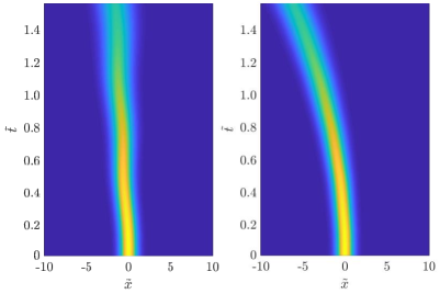
in agreement with Eq. (17). The left side of Fig. 1 shows an example, where $f(t)=\ell\sin(\omega t)$. The center of mass of the wavepacket is located at $\xi(t)=\frac{\ell}{m\omega^{2}}\left[\sin(\omega t)-\omega t\right]$, and it spreads according to Eq. (42). We use the parameterization $\ell=l\cdot\tilde{\ell}$ and $\omega=u\cdot\tilde{\omega}$, where $\tilde{\ell}$ and $\tilde{\omega}$ are dimensionless, and define $\tilde{t}=t/u$ and $\tilde{x}=x\sqrt[3]{\frac{ml}{\hbar^{2}}}$. In the left side of Fig. 1 we set: $\tilde{\sigma}=\sigma\sqrt[3]{\frac{ml}{\hbar^{2}}}=2^{-1/2}$, $\tilde{\ell}=10$, and $\tilde{\omega}=10$.

Figure 1: Time evolution of density profiles of Gaussian wavepackets $\left|\chi(x,t)\right|^{2}$ for a single particle in a potential: $xf(t)$. The left plot shows an evolution with a driving force $f(t)=\ell\sin(\omega t)$: the motion proceeds with a constant stroboscopic velocity towards the left. The right plot shows the evolution under a driving force $f(t)=\ell\sin^{2}(\omega t)$: the motion is uniformly accelerated to negative values of $x$. The figures are calculated via the split-step Fourier method and in both $\tilde{\sigma}=2^{-1/2}$, $\tilde{\ell}=10$, and $\tilde{\omega}=10$.

II.2.2 $\boldsymbol{\int_{0}^{T}f(t)\,dt\neq 0}$

In this case, the independence of the Floquet Hamiltonian (II.2) on $n$ is more difficult to demonstrate. Let us define a function $F(t)$, such that $\frac{dF}{dt}=f(t)$. We have $\int_{0}^{T}f(t)\,dt=F(T)=c$, where $c$ depends on the driving parameters and, by definition, $F(0)=0$. It follows that $F(nT)=nF(T)=nc$. It is easy to prove that $F(t+T)=F(T)+F(t)=c+F(t)$. Therefore $F(nT+t)=nc+F(t)$ and $\xi(nT)$ can be written as

$$\xi(nT)=-\frac{1}{m}\int_{0}^{nT}F(t)\,dt=-\frac{n^{2}}{m}I\,,$$ (43)

where $I=\int_{0}^{T}F(t)\,dt$. Thus $\xi(nT)$ depends quadratically on the stroboscopic factor $n$, and the stroboscopic motion experiences a uniform acceleration $-\frac{1}{m}I$. Next, since $\xi(nT)\propto n^{2}$, one has $\xi(-T)=\xi(T)$ and, choosing $n=-1$ in Eq. (29), yields: $\xi(T)=-\frac{T}{2m}\int_{0}^{T}f(t)\,dt$. This can be substituted back into Eq. (29) to obtain

$$\xi(nT)=-\frac{n^{2}T}{2m}\int_{0}^{T}f(t)\,dt\,.$$ (44)

If we now take $t=nT$ in (26) and use (44), we derive the relevant equation

$$\int_{0}^{nT}d\tau\int_{0}^{\tau}f(\tau^{\prime})\,d\tau^{\prime}\,=\,\frac{n^{2}T}{2}\int_{0}^{T}f(t)\,dt\,,$$

that holds when the integral of the driving function over a driving period does not vanish. Using these results into (II.2), we can write

$$\hat{H}_{F}=\frac{\hat{p}^{2}}{2m}-\hbar\frac{\theta(x,T)}{T}-\frac{1}{6m}\left[\int_{0}^{T}f(\tau)\,d\tau\right]^{2}\,,$$ (45)

or, equivalently,

$$\hat{H}_{F}=\frac{\hat{p}^{2}}{2m}+x\,\frac{1}{T}\int_{0}^{T}f(\tau)\,d\tau+\frac{1}{2m}\frac{1}{T}\int_{0}^{T}d\tau\left[\int_{0}^{\tau}f(\tau^{\prime})\,d\tau^{\prime}\right]^{2}-\frac{1}{6m}\left[\int_{0}^{T}f(\tau)\,d\tau\right]^{2}\,.$$

This expression is independent on $n$, a fact which completes the proof. Unlike the case where $\int_{0}^{T}f(t)\,dt=0$, the Floquet Hamiltonian does not contain a term proportional to $\hat{p}$, but a static linear potential. This term forces the particle to move to the left/right for positive/negative values of $\int_{0}^{T}f(t)\,dt$. An example is given in Fig. 1-right where $\frac{1}{T}\int_{0}^{T}f(\tau)\,d\tau=\frac{\ell T}{2}>0$, so that the wavepacket moves with an acceleration of $-\frac{\ell T^{2}}{4m}$. However, its spread does not depends on the external driving force as predicted in Eq. (17).

The eigenfunctions of the Floquet Hamiltonian are the Airy function $Ai$ LandauLif of the form:

$$\tilde{u}(x)=CAi\left\{\left(\frac{2mT^{2}}{\hbar^{2}\left[\int_{0}^{T}f(\tau)\,d\tau\right]^{2}}\right)^{1/3}\,\left(\frac{x}{T}\int_{0}^{T}f(\tau)\,d\tau-\mathcal{E}_{F}+\Omega\right)\right\}\,,$$ (46)

where $C$ is a normalization constant and

$$\Omega=\frac{1}{2m}\frac{1}{T}\int_{0}^{T}d\tau\left[\int_{0}^{\tau}f(\tau^{\prime})\,d\tau^{\prime}\right]^{2}-\frac{1}{6m}\left[\int_{0}^{T}f(\tau)\,d\tau\right]^{2}\,.$$

The Floquet Hamiltonian has a continuous spectrum spanning the whole range of energy values $\mathcal{E}_{F}$ from $-\infty$ to $+\infty$.

The micro-motion operator is obtained inverting Eq. (2), and it leads to

$$\hat{U}_{F}(t,0)=e^{\frac{i}{\hbar}\left\{t\hbar\left[\frac{\theta(x,t)}{t}-\frac{\theta(x,T)}{T}\right]-\frac{t}{2m}\int_{0}^{T}f(\tau)\,d\tau\cdot\left[\frac{1}{3}\left(1+2\frac{t^{2}}{T^{2}}\right)\int_{0}^{T}f(\tau)\,d\tau\right]-\xi(t)\frac{t}{T}\int_{0}^{T}f(\tau)\,d\tau\right\}}\,e^{-\frac{i}{\hbar}\left[\xi(t)+\frac{t^{2}}{2mT}\int_{0}^{T}f(\tau)\,d\tau\right]\hat{p}}\,.$$ (47)

This expression makes it complicated to determine the time evolution, even for a Gaussian wavepacket, using Eq.(24). To circumvent this problem we perform the unitary transformation

$$\chi(x,t)=\hat{U}_{F}(t,0)\tilde{\chi}(x,t)\,,$$

where the transformed wavefunction satisfies Holthaus2016

$$i\hbar\frac{\partial\tilde{\chi}}{\partial t}=\hat{H}_{F}\tilde{\chi}(x,t)\,.$$

Since $\hat{H}_{F}$ has a linear potential term, we can apply the same reasoning used to solve the original equation (5) for a constant driving function $\tilde{f}=\frac{1}{T}\int_{0}^{T}f(\tau)\,d\tau$, therefore we translate and gauge transform the wavefunction $\tilde{\chi}(x,t)$ in order to wash out the $x$-linear term in the Floquet Hamiltonian. By doing so, we finally get Eq. (14), which is thus the convenient way to obtain the time–evolved wavepacket. In summary, we need first to calculate the free expansion of $\chi(x,0)$, then to translate the solution and finally to multiply it by the gauge phase.

The detailed analysis performed so far is valid for a single particle subjected to a linear potential which varies periodically in time. We shall show below that it can be extended straightforwardly to two- or many-particles interacting with a generic interacting potential $V_{2b}(x_{j}-x_{i})$.

III Introducing interactions: The two-body problem

Let us now consider a one–dimensional system of two interacting particles subjected to a linear time–periodic potential. The Schrödinger equation reads

$$i\,\hbar\,\frac{\partial\chi}{\partial t}=\sum_{j=1}^{2}\left[-\frac{\hbar^{2}}{2\,m}\frac{\partial^{2}}{\partial x_{j}^{2}}+x_{j}\,f(t)\right]\chi+V_{2b}(x_{2}-x_{1})\chi\,,$$ (48)

where $V_{2b}(x_{2}-x_{1})$ is a generic potential between the two particles. To solve the Schrödinger equation (48), we can employ the same method discussed in the previous Section: First we perform the gauge transformation

$$\chi(x_{1},x_{2},t)=\,e^{i\left[\theta(x_{1},t)+\theta(x_{2},t)\right]}\eta(y_{1}(t),y_{2}(t),t)\,,$$ (49)

where $y_{j}(t)=x_{j}-\xi(t)$, for $j=1,2$. The wavefunction $\eta(y_{1},y_{2},t)$ satisfies the Schrödinger equation for two interacting particles with no external potential:

$$i\hbar\frac{\partial\eta}{\partial t}=-\frac{\hbar^{2}}{2\,m}\left[\frac{\partial^{2}}{\partial y_{1}^{2}}+\frac{\partial^{2}}{\partial y_{2}^{2}}\right]\eta+V_{2b}(y_{2}-y_{1})\,\eta\,,$$ (50)

while $\xi(t)$ and $\theta(x_{j},t)$ obey Eqs. (26) and (12), once we use the same initial conditions of the previous case.

Notice that $V_{2b}(y_{1}-y_{2})\,=\,V_{2b}(x_{1}-x_{2})$, because $y_{j}(t)=x_{j}-\xi(t)$. Moreover, since $\xi(0)=0$, the two wavefunctions coincide at initial time: $\chi(x_{1},x_{2},0)\,=\,\eta(x_{1},x_{2},0)$, hence the solution of (48) can be written as

$$\chi(x_{1},x_{2},t)\,=\,e^{i\theta(x_{1},t)+i\theta(x_{2},t)}e^{-i\frac{\xi(t)}{\hbar}(\hat{p}_{1}+\hat{p}_{2})}e^{-i\frac{t}{\hbar}\left[\frac{\hat{p}_{1}^{2}+\hat{p}_{2}^{2}}{2m}+V_{2b}(x_{2}-x_{1})\right]}\,\chi(x_{1},x_{2},0)\,.$$ (51)

With this expression, using the procedure discussed in the previous Section, we can compute the expectation values of physical observables and their variances. More precisely, the expectation value of a single particle operator $\hat{O}_{j}$ is defined as

$$\left\langle\hat{O}_{j}\right\rangle(t)\equiv\left\langle\chi(x_{1},x_{2},t)\left|\hat{O}_{j}\right|\chi(x_{1},x_{2},t)\right\rangle=\int_{-\infty}^{\infty}dx_{1}\int_{-\infty}^{\infty}dx_{2}\,\chi^{*}(x_{1},x_{2},t)\,\hat{O}_{j}\,\chi(x_{1},x_{2},t)\,,$$ (52)

and expectation values of position and momentum can be computed using the Baker-Campbell-Hausdorff formula.

We will show below that there is a decoupling between the linear potential term and the interacting one. This decoupling arises from the separation of the center of mass motion (which is determined by the external potential), and the relative motion (determined by the interacting potential). The diffusion of the wavepacket evolves as it would be free from the linear time dependent potential, but of course depends on the interaction.

The undriven Hamiltonian is given by

$$\hat{H}_{0}=\frac{\hat{p}_{1}^{2}+\hat{p}_{2}^{2}}{2m}+V_{2b}(x_{2}-x_{1})\,.$$

This implies that the total momentum of the system $\hat{P}=\hat{p}_{1}+\hat{p}_{2}$ is conserved, i.e. $\left[\hat{H}_{0},\hat{P}\right]=0$. An example is the contact interaction $V_{2b}(x_{2}-x_{1})\,=\,\lambda\,\delta(x_{2}-x_{1})$, with $\lambda$ the coupling strength. This property allows us to calculate the total energy of the state:

$$E(t)=\left\langle\hat{H}\right\rangle(t)=\left\langle\chi(x_{1},x_{2},t)\left|\left[\frac{\hat{p}_{1}^{2}+\hat{p}_{2}^{2}}{2m}+f(t)\left(x_{1}+x_{2}\right)+V_{2b}\left(x_{2}-x_{1}\right)\right]\right|\chi(x_{1},x_{2},t)\right\rangle\,.$$ (53)

After a lengthy calculation, using the canonical commutation relations and Eq. (51), we obtain for a generic driving function $f(t)$, including as well the non-periodic cases:

$$E(t) = E(0)+\frac{1}{m}\left[\int_{0}^{t}f(\tau)d\tau\right]^{2}+\sum_{j=1}^{2}p_{0,j}\left[\frac{t}{m}f(t)-\frac{1}{m}\int_{0}^{t}f(\tau)d\tau\right]+$$

$$-\frac{2f(t)}{m}\int_{0}^{t}d\tau\int_{0}^{\tau}f(\tau^{\prime})d\tau^{\prime}+\sum_{j=1}^{2}x_{0,j}\left[f(t)-f(0)\right]\,,$$

where $E(0)$ is the initial energy of the state, containing all the interaction effects. The remaining terms arise from the linear driving potential and depend on the position $x_{0,j}$ and momenta $p_{0,j}$, of the $j$-th particle at time $t=0$. If $f(t)$ is constant, as for a constant (gravitational or electric) force, then the energy is conserved. On the other hand, if $f(t)$ is periodic, its integral over a time–period vanishes, and $f(t=0)=0$, then the energy is conserved at stroboscopic times.

Next we shall study the models where $f(t)$ is periodic. As done in the previous Section, we shall consider two cases: $\int_{0}^{T}f(t)\,dt=0$, and $\int_{0}^{T}f(t)\,dt\neq 0$. The evolution operator can be read from (51):

$$\hat{U}(t,0)\,=\,e^{i\left[\theta(x_{1},t)+\theta(x_{2},t)\right]}e^{-i\frac{\xi(t)}{\hbar}(\hat{p}_{1}+\hat{p}_{2})}e^{-i\frac{t}{\hbar}\left[\frac{\hat{p}_{1}^{2}+\hat{p}_{2}^{2}}{2m}+V_{2b}(x_{2}-x_{1})\right]}\,.$$ (55)

It is convenient to use the center of mass and relative coordinates: $x=x_{2}-x_{1}$ and $X=\frac{x_{1}+x_{2}}{2}$. In these variables the effects of the linear time dependent potential and the interactions are completely decoupled. The time evolution in these coordinates reads

$$\hat{U}(t,0)=\hat{U}^{\rm com}(t,0)\hat{U}^{\rm rel}(t,0)=e^{-\frac{i}{\hbar}\left\{2X\int_{0}^{t}f(\tau)\,d\tau+\frac{1}{m}\int_{0}^{t}d\tau\left[\int_{0}^{\tau}f(\tau^{\prime})\,d\tau^{\prime}\right]^{2}\right\}}e^{-i\frac{\xi(t)}{\hbar}\hat{P}}e^{-i\frac{t}{\hbar}\frac{\hat{P}^{2}}{4m}}e^{-i\frac{t}{\hbar}\left[\frac{\hat{p}^{2}}{m}+V_{2b}(x)\right]}\,,$$ (56)

where ${\hat{P}}$ is the total momentum, that commutes with the undriven Hamiltonian, and $\hat{p}=\hat{p}_{2}-\hat{p}_{1}$, is the relative momentum of the particles.

III.0.1 $\boldsymbol{\int_{0}^{T}f(t)\,dt=0}$

In this case one finds

$$\hat{H}_{F}=\sum_{j=1}^{2}\left[\frac{\hat{p}_{j}^{2}}{2\,m}+\frac{\xi(T)}{T}\hat{p}_{j}-\hbar\frac{\theta(T)}{T}\right]+V_{2b}(x_{2}-x_{1})\,,$$ (57)

where $\theta(x_{j},T)=\theta(T)$, as follows from Eq. (12).

From the analysis performed so far, and for the similarities with the one-body case, we know that the stroboscopic motion described by the Floquet Hamiltonian occurs with a constant velocity, since the translational parameter is: $\xi(nT)\propto n$. Notice that if the Schrödinger equation with the original undriven Hamiltonian is solvable, then also the Floquet Hamiltonian associated to the motion under the action of a linear time dependent potential is solvable, since it is described by the same two-body potential of the original problem with no driving, apart from a momentum shift. We observe that it is not convenient to solve the dynamics via Eq. (24) with respect to the eigenfunctions of the Floquet Hamiltonian in Eq. (57), while it is instead more advantageous to pass to relative and center of mass coordinates. Using the center of mass and relative coordinates the Floquet Floquet Hamiltonian decouples in two parts

$$\hat{H}_{F}^{\rm com}=\frac{\hat{P}^{2}}{4m}+\frac{\xi(T)}{T}\hat{P}-2\hbar\frac{\theta(T)}{T}\,,$$ (58)

and

$$\hat{H}_{F}^{\rm rel}=\frac{\hat{p}^{2}}{m}+V_{2b}(x)\,.$$ (59)

The same factorization occurs for the micro-motion operators, by defining

$$\hat{U}(t,0)=\hat{U}_{F}^{\rm com}(t,0)e^{-i\frac{t}{\hbar}\hat{H}_{F}^{\rm com}}\,\hat{U}_{F}^{\rm rel}(t,0)e^{-i\frac{t}{\hbar}\hat{H}_{F}^{\rm rel}}\,.$$ (60)

Using Eq. (56), the micro-motion operator for the center of mass evolution has a form

$$\hat{U}_{F}^{\rm com}(t,0)=e^{-it\left\{\frac{2X}{\hbar t}\int_{0}^{t}f(\tau)\,d\tau+\frac{1}{m\hbar t}\int_{0}^{t}d\tau\left[\int_{0}^{\tau}f(\tau^{\prime})\,d\tau^{\prime}\right]^{2}+2\frac{\theta(T)}{T}\right\}}\,e^{i\frac{t}{\hbar}\left[\frac{\xi(T)}{T}-\frac{\xi(t)}{t}\right]\hat{P}}\,,$$ (61)

while the micro-motion operator for the relative coordinate is instead trivial,

$$\hat{U}_{F}^{\rm rel}(t,0)=\hat{\mathbbm{1}}\,.$$ (62)

The time evolution for the relative motion depends of course on the interacting potential $V_{2b}(x)$. Concerning the center of mass motion, we notice the similarity of Eq. (58) with the Floquet Hamiltonian (31) for a single particle, that allow us to use the results of the previous Section. The eigenfunctions of the Floquet Hamiltonian (58) are plane waves with a continuous spectrum of quasi-energies:

$$\tilde{u}^{\rm com}(X)=\frac{1}{\sqrt{2\pi}}e^{iKX}\,,\,\,\,\,\,\,\,\,\,\,\,\,\,\,\mathcal{E}_{F}^{\rm com}=\frac{\hbar^{2}K^{2}}{4m}+\frac{\xi(T)}{T}\hbar K-2\hbar\frac{\theta(T)}{T}\,,$$ (63)

where $K$ is the center of mass momentum. Next, we can get the Floquet modes by applying $\hat{U}_{F}^{\rm com}(t,0)$ onto $\tilde{u}^{\rm com}(X)$, obtaining

$${u}^{\rm com}(X,t)=\frac{1}{\sqrt{2\pi}}e^{iX\left[K-\frac{2}{\hbar}\int_{0}^{t}f(\tau)\,d\tau\right]}\,e^{-it\left\{\frac{1}{m\hbar t}\left[\int_{0}^{t}d\tau\left(\int_{0}^{\tau}f(\tau^{\prime})\,d\tau^{\prime}\right)^{2}-\frac{2t}{T}\int_{0}^{T}d\tau\left(\int_{0}^{\tau}f(\tau^{\prime})\,d\tau^{\prime}\right)^{2}\right]+K\left[\frac{\xi(t)}{t}-\frac{\xi(T)}{T}\right]\right\}}\,,$$ (64)

where we used Eq. (12). As in the one-body problem, the Floquet modes are plane waves with a momentum varying in time as

$$\left\langle u(t)\left|\hat{K}\right|u(t)\right\rangle\,=\,K-\frac{2}{\hbar}\int_{0}^{t}f(\tau)\,d\tau\,,$$

which implies that $\left\langle K\right\rangle(nT)=K$. We finally get the Floquet states from Eq. (23) and (63),

$$\psi_{F}^{\rm com}(X,t)=\frac{1}{\sqrt{2\pi}}e^{i\left\{KX-\frac{2X}{\hbar t}\int_{0}^{t}f(\tau)\,d\tau-\frac{1}{m\hbar t}\int_{0}^{t}d\tau\left[\int_{0}^{\tau}f(\tau^{\prime})\,d\tau^{\prime}\right]^{2}\right\}-it\frac{\hbar K^{2}}{4m}-iK\xi(t)}\,,$$ (65)

that are plane waves, periodic in time with period $T$, and whose average center of mass momentum behaves like that of the Floquet modes. Therefore the center of mass component of the wavefunction, solution of (48), reads as

$$\phi(X,t)=\int A(K)\psi_{F}^{\rm com}(X,t)\,dK\,,$$ (66)

where we have written: $\chi(x_{1},x_{2},t)=\phi(X,t)\varphi(x,t)$.

III.0.2 $\boldsymbol{\int_{0}^{T}f(t)\,dt\neq 0}$

Using the methods presented in previous Sections, we find

$$\hat{H}_{F}=\sum_{j=1}^{2}\left[\frac{\hat{p}_{j}^{2}}{2m}-\hbar\frac{\theta(x_{j},T)}{T}\right]-\frac{1}{3m}\left[\int_{0}^{T}f(\tau)\,d\tau\right]^{2}+V_{2b}(x_{2}-x_{1})\,.$$ (67)

This expression contains a linear potential, hidden in the gauge phases $\theta(x_{j},T)$. Analogously to the one-body example, the stroboscopic motion of the particles is uniformly accelerated,

$$\frac{d^{2}\left\langle x_{j}\right\rangle}{dt^{2}}(nT)\,=\,-\frac{1}{m}\int_{0}^{T}d\tau\int_{0}^{\tau}f(\tau^{\prime})\,d\tau^{\prime}\,.$$

Using the center of mass and relative coordinates, the Floquet Hamiltonian (67) splits in two parts

$$\hat{H}_{F}^{\rm com}=\frac{\hat{P}^{2}}{4m}+\hat{X}\frac{1}{T}\int_{0}^{T}f(\tau)\,d\tau+\frac{1}{m}\frac{1}{T}\int_{0}^{T}d\tau\left[\int_{0}^{\tau}f(\tau^{\prime})\,d\tau^{\prime}\right]^{2}-\frac{1}{3m}\left[\int_{0}^{T}f(\tau)\,d\tau\right]^{2}\,,$$ (68)

while the Floquet Hamiltonian of the relative motion is given by Eq. (59). The difference between the cases (1) and (2) stems only from the center of mass motion which has an additional linear dependence on $\hat{P}$ in the first case, and $\hat{X}$ in the second. The micro-motion operator can be split as well, obtaining Eq. (62) for the relative part, and

$$\hat{U}_{F}^{\rm com}(t,0)=e^{\frac{i}{\hbar}\big{\{}t\left[X\left(\frac{1}{T}\int_{0}^{T}f(\tau)\,d\tau-\frac{1}{t}\int_{0}^{t}f(\tau)\,d\tau\right)+\frac{1}{mT}\int_{0}^{T}d\tau\left[\int_{0}^{\tau}f(\tau^{\prime})\,d\tau^{\prime}\right]^{2}+\frac{1}{mt}\int_{0}^{t}d\tau\left[\int_{0}^{\tau}f(\tau^{\prime})\,d\tau^{\prime}\right]^{2}\right]+}\\ {}^{-\frac{t}{m}\int_{0}^{T}f(\tau)\,d\tau\cdot\left[\frac{1}{3}\left(1+2\frac{t^{2}}{T^{2}}\right)\int_{0}^{T}f(\tau)\,d\tau\right]+-2\xi(t)\frac{t}{T}\int_{0}^{T}f(\tau)\,d\tau\big{\}}}\,e^{-\frac{i}{\hbar}\hat{P}\left[\xi(t)+\frac{t^{2}}{2mT}\int_{0}^{T}f(\tau)\,d\tau\right]}\,,$$ (69)

for the center of mass.

The dynamics of the relative part can be analysed once the two-body potential is given, while the analysis performed on the center of mass part follows the same line of the one-body case. By this we mean that one has to perform a unitary transformation on the center of mass wavefunction: $\Phi(X,t)=\hat{U}_{F}\tilde{\Phi}(X,t)$, and therefore the new wavefunction $\tilde{\Phi}(X,t)$ satisfies a time dependent Schrödinger equation with the Floquet Hamiltonian (68). Washing away the $X$-linear dependence of the Floquet Hamiltonian by means of a translation and a gauge transformation, for the center of mass part of Eq. (51) we have

$$\Phi(X,t)=e^{-\frac{i}{\hbar}\left\{2X\int_{0}^{t}f(\tau)\,d\tau+\frac{1}{m}\int_{0}^{t}d\tau\left[\int_{0}^{\tau}f(\tau^{\prime})\,d\tau^{\prime}\right]^{2}\right\}}e^{-i\frac{\xi(t)}{\hbar}\hat{P}}e^{-i\frac{t}{\hbar}\frac{\hat{P}^{2}}{4m}}\,\Phi(X,0)\,,$$ (70)

where Eq. (56) has been used.

As an example, we use the above results to study the time evolution of two particles with contact interactions initially prepared in a Gaussian wavepacket.

III.1 Contact interactions

Let consider a contact potential: $V_{2b}(x_{2}-x_{1})=\lambda\delta(x_{2}-x_{1})$, where $\lambda>0$ is the repulsive interaction parameter. At the initial time we prepare a Gaussian wavepacket with variance $\sigma$

$$\chi(x_{1},x_{2},0)=\frac{1}{\sqrt{\pi\sigma^{2}}}e^{-\left(x_{1}^{2}+x_{2}^{2}\right)/2\sigma^{2}}\,,$$ (71)

that factorizes into the center of mass and relative parts

$$\Phi(X,0)=\sqrt[4]{\frac{2}{\pi\sigma^{2}}}e^{-X^{2}/\sigma^{2}}\,\,\,\,\,\,,\,\,\,\,\,\,\,\,\,\,\,\,\,\,\,\,\,\varphi(x,0)=\frac{1}{\sqrt[4]{2\pi\sigma^{2}}}e^{-x^{2}/4\sigma^{2}}\,.$$ (72)

Let us start with the case: $\int_{0}^{T}f(\tau)\,d\tau=0$. Finding the time–independent coefficient $A(K)$ appearing in Eq. (66) at $t=0$, and using (72), yields:

$$\Phi(X,t)=\sqrt[4]{\frac{2}{\pi\sigma^{2}}}\,\frac{e^{i\theta(X,t)}}{\sqrt{1+i\frac{\hbar\,t}{m\sigma^{2}}}}\,\,e^{-\frac{\left[X-\xi(t)\right]^{2}}{\sigma^{2}\left(1+i\frac{\hbar\,t}{m\sigma^{2}}\right)}}\,.$$ (73)

Concerning the relative motion, we use the propagator $G(x,x^{\prime};t,0)$ in the presence of a Dirac $\delta$-potential Bauch1985 ; Andreata2004

$$\varphi(x,t)=\int_{-\infty}^{\infty}G(x,x^{\prime};t,0)\,\varphi(x^{\prime},0)\,dx^{\prime}\,,$$ (74)

with

$$G(x,x^{\prime};t,0)=\frac{1}{\sqrt{4\,\pi\,i\,\hbar\,t/m}}\,e^{i\,\frac{m\,(x-x^{\prime})^{2}}{4\,\hbar\,t}}-\frac{m\,\lambda}{4\,\hbar^{2}}\,e^{\frac{m\,\lambda}{2\,\hbar^{2}}\left(\left|x\right|+\left|x^{\prime}\right|\right)+i\,\frac{m\,\lambda^{2}\,t}{4\,\hbar}}\,{\rm erfc}\left(\frac{\left|x\right|+\left|x^{\prime}\right|+i\frac{\lambda\,t}{\hbar}}{\sqrt{4\,i\,\hbar\,t/m}}\right)\,,$$ (75)

with ${\rm erfc}$ being the complementary error function:

$${\rm erfc}(z)=\frac{2}{\sqrt{\pi}}\int_{z}^{\infty}e^{-t^{2}}\,dt\,.$$

The numerical integration of (74), provides the wavefunction $\chi(x_{1},x_{2},t)$ for any value of $\lambda>0$. In the limit of hard–core interactions, $\lambda\to\infty$, the integral (74) can be computed analytically

$$\varphi(x,t)=\frac{1}{\left(2\pi\right)^{1/4}}\sqrt{\frac{im\sigma/\hbar t}{-1+im\sigma^{2}/\hbar t}}\,\,{\rm erf}\left(\frac{m\,\sigma\,x}{2\hbar t\sqrt{-1+im\sigma^{2}/\hbar t}}\right)\,e^{-\frac{m}{4\hbar t}\frac{x^{2}}{i+m\sigma^{2}/\hbar t}}\,,$$ (76)

where ${\rm erf}(z)=1-{\rm erfc}(z)$. We have studied the time evolution of the density matrix

$$\rho(x_{1},t)=2\,\int_{-\infty}^{\infty}\left|\chi(x_{1},x_{2},t)\right|^{2}\,dx_{2}\,,$$ (77)

in order to visualize the evolution of the wavepacket. The density matrix (77) reads in the center of mass and relative wavefunctions, as

$$\rho(x,t)=2\,\int_{-\infty}^{\infty}\left|\Phi\left(\frac{x_{1}}{2}+x,t\right)\right|^{2}\,\left|\varphi(x_{1},t)\right|^{2}\,dx_{1}\,,$$ (78)

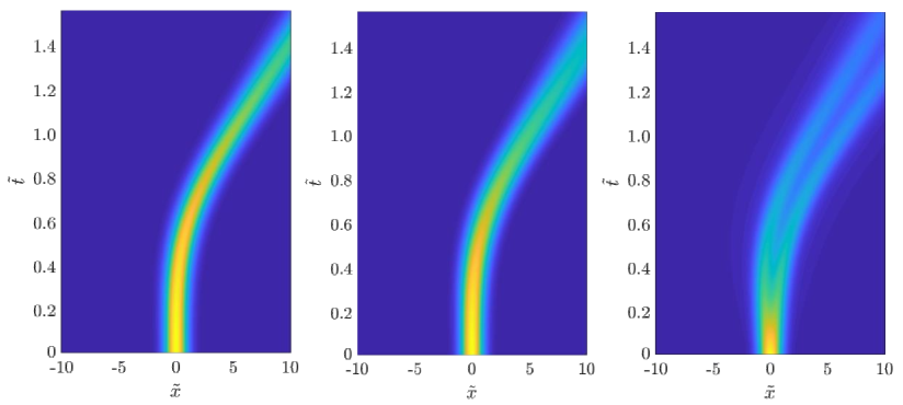
The results are reported in Fig. 2 for different times and coupling strengths $\lambda$, using the driving function

$$f(t)=\ell\left[\cos^{2}(\omega t)-1+\frac{4}{3}\sin^{4}(\omega t)\right]\,.$$

We choose the same dimensionless variables as in the one-body case: dimensionless coupling strength $\tilde{\lambda}=l\frac{m\lambda}{\hbar^{2}}$, $\tilde{\ell}=200$, $\tilde{\omega}=2$ and $\tilde{\sigma}=1$. The values $\tilde{\lambda}=0$, $1$ and $\infty$, correspond to the left, center and right sides of Fig. 2. Here

$$\xi(t)=\frac{\ell}{12m\omega^{2}}\sin^{4}(\omega t)\,,$$

vanishes at stroboscopic times, as checked in the numerical simulations. We have also verified that the wave packet expands as it were not subjected to the linear oscillating potential, in agreement with the theoretical prediction.

Fig. 2 shows that increasing the parameter $\lambda$, the variance of the wavepacket increases in time more rapidly. We have been able to fit this behaviour with the approximation

$$\Delta x_{j}(t)\approx\frac{\sigma}{\sqrt{2}}\sqrt{1+\left(\frac{\hbar\,t}{m\,\sigma^{2}}\right)^{2}\left(1+{\cal B}\,\frac{m\,\lambda\,\sigma}{2\,\hbar^{2}}\right)}\,,$$ (79)

where ${\cal B}\approx 1.23$. For $\lambda=0$ one retrieves an expression similar to Eq. (42), while in the limit $\lambda\rightarrow\infty$, Eq. (79) diverges for all $t$ because the tail of the density matrix decays as $\propto\/x^{2}$, even starting from a Gaussian.

Figure 2: Time evolution of density matrix profiles (77) for a Gaussian wavepacket (71), under the action of a linear external potential: $xf(t)$, with driving function $f(t)=\ell\left[\cos^{2}(\omega t)-1+\frac{4}{3}\sin^{4}(\omega t)\right]$. The left side plot is the free case, $\tilde{\lambda}=0$, the central plot has $\tilde{\lambda}=1$, while the right side plot has $\tilde{\lambda}=\infty$. The center of mass moves with constant stroboscopic velocity, as predicted analytically, and the wavepacket spreads over time as it would do for the undriven case $\ell=0$. As one can see from the right side plot, for very large interactions, the wavepacket rapidly tends to split in two specular parts. In all the figures the values $\tilde{\ell}=200$, $\tilde{\omega}=2$ and $\tilde{\sigma}=1$ have been chosen.

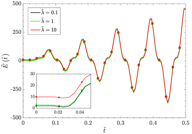
As an additional check, we have calculated numerically the total energy of a two-particle system driven with $f(t)=\ell\sin^{3}(\omega t)$, separating its center of mass and relative components. The analytical value can be obtained from Eq. (III), and is represented by the solid lines in Fig. 3. The dots represent the values calculated numerically. We have used $\tilde{\ell}=200$, $\tilde{\omega}=60$, $\tilde{\sigma}=2^{-1/2}$ and $p_{0,j}=x_{0,j}=0$ for $j=1$, $2$. The interaction strengths, $\tilde{\lambda}=0.1$, $1$ and $10$, only displace the curves since their effects are encoded in the initial energy factor $E(0)$ of Eq. (III), as can be seen from the inset of the plot. For this driving function we have $f(nT)=\int_{0}^{T}f(\tau)\,d\tau=0$, therefore from Eq. (III) the energies at the stroboscopic times are equal to the initial energy, i.e. $E(nT)=E(0)$ for every $n$, and there is no heating of the system, in agreement with theoretical results Sierra2015 ; He2019 and experimental findings Pandey2019 .

Figure 3: Time evolution of the energy $\tilde{E}=\sqrt[3]{\frac{m}{\hbar^{2}l}}\,E$ for two interacting particles subjected to a linear external potential: $xf(t)$, with driving function $f(t)=\ell\sin^{3}(\omega t)$. The system is prepared in the Gaussian wavepacket state (71). The curves represent different values of the parameter $\tilde{\lambda}$, which only shifts the total energy, as shown in the inset for short times $\tilde{t}$ and different coupling strengths. The dots represent the energy values calculated from the numerical computation.

In the case where $\int_{0}^{T}f(\tau)\,d\tau\neq 0$, we used Eq. (70) for the center of mass initial wavefunction of Eq. (72), obtaining the same result as when $\int_{0}^{T}f(\tau)\,d\tau=0$, i.e. we retrieved Eq. (73). For the relative motion we have applied the same reasoning as before, by which we know that the relative part of the wavepacket evolves according to Eq. (74). We have performed a numerical simulation of a system made of two $\delta$-interacting particles under the action of a linear potential with driving function: $f(t)=\ell\left[\cos(\omega t)-1\right]$. The results for different interaction strengths $\lambda$ are reported in Fig. 4, where the density matrices calculation (78) is plotted, in correspondence of $\tilde{\ell}=10$, $\tilde{\omega}=5$ and $\tilde{\sigma}=1$. In this case the motion is uniformly accelerated to the right side of the $x$-axis, indeed the translational parameter reads $\xi(t)=\frac{\ell}{2m\omega^{2}}\left[\omega^{2}t^{2}-2+2\cos(\omega t)\right]$. This has to be compared with the the case $\int_{0}^{T}f(t)\,dt=0$, where the center of mass does not accelerate.

Concerning the spreading of the wavepacket, it is the same as in the case without a driving potential and it also satisfies Eq. (79) with ${\cal B}\approx 1.23$. In conclusion, there is no difference for the wavepacket spreading between the results of a driving function whose integral over a period vanishes or not.

Figure 4: Evolution of density matrix (77) for a Gaussian wavepacket (71) under the action of a linear external potential: $xf(t)$, where the driving function is $f(t)=\ell\left[\cos(\omega t)-1\right]$. Notice that the center of mass motion is uniformly accelerated to the right, as predicted analytically, and the wavepacket spreads over time as it would do for the undriven case. From left to right panels one has $\tilde{\lambda}=0,1,\infty$; moreover, $\tilde{\ell}=10$, $\tilde{\omega}=5$ and $\tilde{\sigma}=1$.

IV Many-body problem

The analysis done so far can be generalized to many-body systems with $N$ interacting particles, a generic interacting potential $V_{2b}(x_{j}-x_{i})$ and under the action of an external linear time–dependent potential. The Schrödinger equation reads

$$i\,\hbar\,\frac{\partial\chi}{\partial t}=\sum_{j=1}^{N}\left[-\frac{\hbar^{2}}{2\,m}\frac{\partial^{2}}{\partial x_{j}^{2}}+x_{j}\,f(t)\right]\chi+\sum_{j>i}V_{2b}(x_{j}-x_{i})\chi\,.$$ (80)

Performing the translation and a gauge transformation

$$\chi(x_{1},\dots,x_{N},t)\equiv\prod_{j=1}^{N}e^{i\theta(x_{j},t)}\eta(y_{1},\dots,y_{N},t)\,,$$ (81)

the wavefunction $\eta(y_{1},\dots,y_{N},t)$ satisfies the Schrödinger equation without the external driving, i.e.

$$i\,\hbar\,\frac{\partial\eta}{\partial t}=-\frac{\hbar^{2}}{2\,m}\sum_{j=1}^{N}\frac{\partial^{2}\eta}{\partial y_{j}^{2}}+\sum_{j>i}V_{2b}(y_{j}-y_{i})\eta\,,$$ (82)

where $y_{j}(t)=x_{j}-\xi(t)$, $\forall j$, therefore the interacting potential is invariant under these transformations: $V_{2b}(y_{j}-y_{i})=V_{2b}(x_{j}-x_{i})$.

Using the initial conditions $\xi(0)=0$ and $\theta(x_{j},0)=0$, $\forall j$, the parameter $\xi(t)$ and the gauge phase $\theta(x_{j},t)$ satisfy Eqs. (26) and (12). Hence, the two wavefunctions coincide at initial time $t=0$.

The complete solution of the Schrödinger equation (80) can be formally written as

$$\chi(x_{1},\dots,x_{N},t)\,=\,\prod_{j=1}^{N}\left[e^{i\theta(x_{j},t)}e^{-i\frac{\xi(t)}{\hbar}\hat{p}_{j}}\right]e^{-i\frac{t}{\hbar}\hat{H}_{0}}\chi(x_{1},\dots,x_{N},0)\,,$$ (83)

where the undriven Hamiltonian of one–dimensional many-particles systems has the general form

$$\hat{H}_{0}=\sum_{j=1}^{N}\frac{\hat{p}_{j}^{2}}{2m}+\sum_{j>i}V_{2b}(x_{j}-x_{i})\,.$$ (84)

In (83) the momentum operator $\hat{p}_{j}$ is the generator of the translation for the $j$-th particle, and $\eta$ is the solution of the Schrödinger equation with no linear driving.

The generalization of the two-body results for the expectation values of physical observables is straightforward. Firstly, we can compute the total energy of the system evaluating the expectation value of the driven Hamiltonian. In the calculation we use the conservation of the total momentum $\hat{P}=\sum_{j=1}^{N}\hat{p}_{j}$ for the undriven Hamiltonian $\hat{H}_{0}$, i.e. $\left[\hat{H}_{0},\hat{P}\right]=0$, valid in the considered case in which the interaction $V_{2b}$ depends on the relative distance between the particles (see more comments in Section IV.1). Using the commutation relations we find for a general (also non-periodic) driving function $f(t)$:

$$E(t) = E(0)+\frac{N}{2m}\left[\int_{0}^{t}f(\tau)d\tau\right]^{2}+\sum_{j=1}^{N}p_{0,j}\left[\frac{t}{m}f(t)-\frac{1}{m}\int_{0}^{t}f(\tau)d\tau\right]+$$

$$-\frac{Nf(t)}{m}\int_{0}^{t}d\tau\int_{0}^{\tau}f(\tau^{\prime})d\tau^{\prime}+\sum_{j=1}^{N}x_{0,j}\left[f(t)-f(0)\right]\,,$$

which generalizes Eq. (III). As for the two-body case, if $f(t)$ is periodic in time and its integral over a time–period vanishes, then the energy is conserved at stroboscopic times if $f(t=0)=0$. Once again, there is a decoupling between the interactions and the external linear driving potential, since the effect of the interactions among particles is encoded in the initial value of the energy $E(0)$, while the remaining terms collect the effect of the external potential.

Let us now focus on periodic driving functions. As before, we discuss separately the cases when $\int_{0}^{T}f(\tau)\,d\tau=0$ and $\neq 0$. In the first case, the gauge phase at stroboscopic times is independent on the position variables, while the parameter $\xi$ is linear in the stroboscopic factor $n$, indicating a stroboscopic motion with constant velocity. Using the fact that $\left[\hat{H}_{0},\hat{P}\right]=0$ and the Baker-Campbell-Hausdorff formula on Eq. (83) evaluated at $t=nT$, we find the Floquet Hamiltonian

$$\hat{H}_{F}=\sum_{j=1}^{N}\left[\frac{\hat{p}_{j}^{2}}{2\,m}+\frac{\xi(T)}{T}\hat{p}_{j}-\hbar\frac{\theta(T)}{T}\right]+\sum_{j<i}V_{2b}(x_{j}-x_{i})\,.$$ (86)

Hence, if the undriven Hamiltonian describes an integrable model, also the Floquet Hamiltonian is exactly solvable since it has the same two-body interaction potential among particles and presents only a shift in the momenta. For the micro-motion operator one finds

$$\hat{U}_{F}(t,0)=e^{it\sum_{j=1}^{N}\left[\frac{\theta\left(x_{j},t\right)}{t}-\frac{\theta(T)}{T}\right]}\,e^{i\frac{t}{\hbar}\left[\frac{\xi(T)}{T}-\frac{\xi(t)}{t}\right]\sum_{j=1}^{N}\hat{p}_{j}}\,.$$ (87)

If $f(t)$ has a non-vanishing integral over a driving period, then the Floquet Hamiltonian reads

$$\hat{H}_{F}=\sum_{j=1}^{N}\left[\frac{\hat{p}_{j}^{2}}{2m}-\hbar\frac{\theta(x_{j},T)}{T}\right]-\frac{N}{6m}\left[\int_{0}^{T}f(\tau)\,d\tau\right]^{2}+\sum_{j<i}V_{2b}(x_{j}-x_{i})\,,$$ (88)

which presents a time–independent $x$-linear potential term acting on all the particles. In this case, as we saw for the one-body problem, the system is governed by a stroboscopic dynamics with a uniform acceleration, since the translational parameter depends quadratically on the stroboscopic factor: $\xi(nT)\propto n^{2}$. The micro-motion operator reads:

$$\hat{U}_{F}(t,0) = e^{\frac{i}{\hbar}\left\{t\hbar\sum_{j=1}^{N}\left[\frac{\theta\left(x_{j},t\right)}{t}-\frac{\theta\left(x_{j},T\right)}{T}\right]-N\frac{t}{2m}\int_{0}^{T}f(\tau)\,d\tau\cdot\left[\frac{1}{3}\left(1+2\frac{t^{2}}{T^{2}}\right)\int_{0}^{T}f(\tau)\,d\tau\right]-N\xi(t)\frac{t}{T}\int_{0}^{T}f(\tau)\,d\tau\right\}}\cdot$$ (89)

$$\cdot\,e^{-\frac{i}{\hbar}\left[\xi(t)+\frac{t^{2}}{2mT}\int_{0}^{T}f(\tau)\,d\tau\right]\sum_{j=1}^{N}\hat{p}_{j}}\,.$$

IV.1 Comments

We pause here to comment on the generality of our findings. The main results in the case $\int_{0}^{T}f(\tau)\,d\tau=0$ are Eqs. (86) and (87). They are valid for any form of the two-body potential $V_{2b}$ and therefore for any interacting Hamiltonian (84), integrable or not. The crucial assumption we have made is that the two-body potential $V_{2b}$ depends only on the relative distance $x_{i}-x_{j}$, otherwise $V_{2b}(x_{i},x_{j})$ would be in general different from $V_{2b}(y_{i},y_{j})$ when the transformation $y_{j}=x_{j}-\xi(t)$ is done. Since $V_{2b}(x_{j}-x_{i})=V_{2b}(y_{j}-y_{i})$ then the equations of motions for the wavefunction $\eta(y_{1},\dots,y_{N},t)$ are exactly the same of those for the wavefunction $\chi(x_{1},\dots,x_{N},t)$, except for the fact that the time–periodic linear potential has been removed. Notice, that in presence of one-body potentials $V_{1b}(x_{i})$, breaking translational invariance, this fact would be no longer valid. When the interacting many-body Hamiltonian has only the kinetic term plus a time–independent two-body potential $V_{2b}$ depending only on the relative distance between the particles, then the conservation of the total momentum of the undriven Hamiltonian $\hat{H}_{0}$ is guaranteed:

$$\left[\hat{H}_{0},\hat{P}\right]=0\,,$$

a relation we subsequently used to determine the Floquet Hamiltonian, the micro-motion operator and the expression of the energy at time $t$.

We conclude that if, in addition, $\hat{H}_{0}$ turns out to be integrable, then the associated Floquet Hamiltonian is integrable too. We have presented the analysis for a many-body systems made of bosons, but it could equally be applied to a many-body systems made of fermions or Bose–Fermi mixtures. In few words, our results are valid for any one–dimensional integrable Hamiltonian in the continuum. This also includes the Gaudin-Yang model for one–dimensional Fermi gases, integrable Bose-Fermi mixtures, integrable multi-component Lieb–Liniger Bose gases and Calogero-Sutherland models (in the absence of external one-body harmonic potential) Korepin1993 ; Sutherland04 ; Mussardo10 ; Gaudin14 .

Hence, having in mind the broad generality of our results, we shall present below a study of the paradigmatic Lieb–Liniger model driven by an external linear time–dependent potential whose driving function has a vanishing integral over a driving period.

IV.2 Driven Lieb–Liniger gas

The Lieb–Liniger model describes a gas of $N$ bosons with $\delta$-contact repulsive interactions in one–dimension LiebLiniger1963 , tha is $V_{2b}(x_{j}-x_{i})=\lambda\delta(x_{j}-x_{i})$, with $\lambda>0$ the interaction parameter. The dynamics of the Lieb–Liniger model in a linear potential was studied in Jukic2010 , while we refer to Chen ; Ablowitz2004 for a study of the classical counterpart of the Lieb–Liniger model, the nonlinear Schrödinger equation, in the presence of a time–dependent linear potential. The Floquet analysis of the Lieb–Liniger model with a periodic tilting was studied in ourPRL2019 , where it was discussed the stroboscopic evolution written in terms of the eigenfunctions of the Floquet Hamiltonian in Eq. (86). Here we make a further step forward, giving a procedure for getting an expression for the time evolution of a generic wavepacket.

The undriven Hamiltonian of this system, i.e.

$$\hat{H}_{0}=\sum_{j=1}^{N}\frac{\hat{p}_{j}^{2}}{2m}+\lambda\sum_{j<i}\delta(x_{j}-x_{i})\,\,\,$$ (90)

is an integrable Hamiltonian and an exact expression of its eigenfunction can be obtained using the Bethe ansatz technique Korepin1993 ; Yang1969 . Therefore we can write the eigenfunctions for the Floquet Hamiltonian (86) as Bethe ansatz states

$$\left|\tilde{u}\right\rangle=\sum_{P}A_{P}(Q)\,e^{\frac{i}{\hbar}\sum_{j=1}^{N}k_{P_{j}}x_{j}}\,,$$ (91)

where $Q$ is the permutation index which specifies the order of the particles, while $P$ is the permutation index of the pseudo-rapidities $k_{j}$, which are undetermined until boundary conditions are chosen Korepin1993 ; Mussardo10 (we refer to ourPRL2019 for a discussion on the relation between the boundary conditions and the external linear potential). The amplitudes $A_{P}(Q)$ can be written as

$$A_{P}=\mathcal{N}\,(-1)^{P}\,\prod_{j<l}\left(k_{P_{j}}-k_{P_{l}}+i\frac{m\lambda}{\hbar^{2}}\right)\,,$$

where $\mathcal{N}$ represents the normalization factor. The respective quasi-energies are given by

$$\mathcal{E}_{F}=\frac{\hbar^{2}}{2m}\sum_{j=1}^{N}k_{j}^{2}+\hbar\frac{\xi(T)}{T}\sum_{j=1}^{N}k_{j}-N\hbar\frac{\theta(T)}{T}\,.$$ (92)

For convenience, we will indicate the state $\tilde{u}$ as ${\rm BAS}(k_{1},\dots,k_{N})$, where ${\rm BAS}$ stands for Bethe Ansatz State. In order to understand what happens for the $N$–body case, it is convenient to start from the two-body problem. In this case we can write FranchiniBook

$${\rm BAS}(k_{1},k_{2})=g(x_{1},x_{2})\theta_{H}(x_{2}-x_{1})+g(x_{2},x_{1})\theta_{H}(x_{1}-x_{2})\,,$$ (93)

where $\theta_{H}(x)$ is the Heaviside step function, while

$$g(x_{1},x_{2})=\left[i(k_{1}-k_{2})-\frac{m\lambda}{\hbar^{2}}\right]\,e^{i\left(k_{1}x_{1}+k_{2}x_{2}\right)}+\left[i(k_{1}-k_{2})+\frac{m\lambda}{\hbar^{2}}\right]\,e^{i\left(k_{2}x_{1}+k_{1}x_{2}\right)}\,.$$

Hence, $g(x_{1}+a,x_{2}+a)=g(x_{1},x_{2})\,e^{ia\left(k_{1}+k_{2}\right)}$ for generic $a$, and the action of the micro-motion operator (87) on the ${\rm BAS}$ will give the following Floquet modes

$$u(t)={\rm BAS}\left(k_{1}-\frac{1}{\hbar}\int_{0}^{t}f(\tau)\,d\tau,k_{2}-\frac{1}{\hbar}\int_{0}^{t}f(\tau)\,d\tau)\right)\,e^{i\left(k_{1}+k_{2}\right)t\left[\frac{\xi(T)}{T}-\frac{\xi(t)}{t}\right]}\,e^{-i\left\{\frac{1}{m\hbar}\int_{0}^{t}d\tau\left[\int_{0}^{\tau}f(\tau^{\prime})\,d\tau^{\prime}\right]^{2}+2\frac{t}{T}\theta(T)\right\}}\,.$$ (94)

Apart from a phase, the Floquet modes are then Bethe ansatz states with shifted pseudomomenta. The Floquet states from Eqs. (23) and (92), read

$$\psi_{F}(t)={\rm BAS}\left(k_{1}-\frac{1}{\hbar}\int_{0}^{t}f(\tau)\,d\tau,k_{2}-\frac{1}{\hbar}\int_{0}^{t}f(\tau)\,d\tau)\right)\,e^{-i\left(k_{1}+k_{2}\right)\xi(t)}\,e^{-\frac{i}{m\hbar}\int_{0}^{t}d\tau\left[\int_{0}^{\tau}f(\tau^{\prime})\,d\tau^{\prime}\right]^{2}}\,,$$ (95)

and the total momentum expectation value of the Floquet states is therefore $\left\langle\hat{P}\right\rangle_{F}(t)=\hbar\left(k_{1}+k_{2}\right)-\frac{2}{\hbar}\int_{0}^{t}f(\tau)\,d\tau$. These results may be easily extended to the many-body case. The Floquet modes can be written as:

$$u(t) = {\rm BAS}\left(k_{1}-\frac{1}{\hbar}\int_{0}^{t}f(\tau)\,d\tau,\dots,k_{N}-\frac{1}{\hbar}\int_{0}^{t}f(\tau)\,d\tau)\right)\,e^{it\left[\frac{\xi(T)}{T}-\frac{\xi(t)}{t}\right]\sum_{j=1}^{N}k_{j}}\cdot$$ (97)

$$\cdot\,e^{-i\left\{\frac{N}{2m\hbar}\int_{0}^{t}d\tau\left[\int_{0}^{\tau}f(\tau^{\prime})\,d\tau^{\prime}\right]^{2}+N\frac{t}{T}\theta(T)\right\}}\,,$$

while the Floquet states read

$$\psi_{F}(t)={\rm BAS}\left(k_{1}-\frac{1}{\hbar}\int_{0}^{t}f(\tau)\,d\tau,\dots,k_{N}-\frac{1}{\hbar}\int_{0}^{t}f(\tau)\,d\tau)\right)\,e^{-i\xi(t)\sum_{j=1}^{N}k_{j}}\,e^{-i\frac{N}{m\hbar}\int_{0}^{t}d\tau\left[\int_{0}^{\tau}f(\tau^{\prime})\,d\tau^{\prime}\right]^{2}}\,.$$ (98)

The total momentum of the Floquet states is then

$$\left\langle\hat{P}\right\rangle_{F}(t)=\hbar\sum_{j=1}^{N}k_{j}-\frac{N}{\hbar}\int_{0}^{t}f(\tau)\,d\tau\,.$$ (99)

In particular one can calculate the time evolution of a generic wavepacket for this system as

$$\chi(x_{1},\dots,x_{N},t)=\int A(k_{1},\dots,k_{N})\,\psi_{F}(t)\,d^{N}k\,,$$ (100)

which is an extension of the one-body equation (24).

It is worth stressing that this is a non-trivial expansion to evaluate: Indeed, once the initial wavepacket has been chosen at $t=0$, one needs to evaluate the time–independent amplitudes $A(k_{1},\dots,k_{N})$ inverting the integral by multiplying by $\psi_{F}^{*}(t)$, and then evaluate the $N$-dimensional integral on the right hand side.

V Conclusions

In this paper we have studied the effect of a time–dependent linear external potential on one–dimensional quantum systems made of one-, two- and many-particles. The potential could physically represent a time varying gravitational linear force, or a time varying electric field acting on the system, therefore its analysis is interesting in many different contexts. The key point of our approach has been to solve the problem for a generic driving function by applying a gauge transformation on the wavefunction and a translation over the position variables. Doing so, we have been able to compute expectation values for different observables such as the center of mass position of a wavepacket and its variance, and the way these observables depend on time. We have observed that the external driving does not affect the spread of a wavepacket, which depends instead only on the interaction effects. This is the result of the decoupling of the external potential which takes place already from the two-particles case, due to the linearity of the potential. This decoupling acts at the level of the center of mass and relative coordinates and can be observed also in the behaviour of the total energy of the system, which oscillates in time depending on the form of the driving function $f(t)$. We derived expressions for the energy of the state at any time also for non-periodic driving function. The system in general does not conserve the energy, apart from some specific cases, e.g. if $f(t)$ is constant in time. However, when $f$ is periodic in time and its integral on a time–period vanishes, plus $f(t=0)=0$, then the energy at stroboscopic times is conserved (notice that, at stroboscopic times, the expectation value of the full Hamiltonian does not need to be equal to the expectation value of the Floquet Hamitonian). When $f$ is periodic, but its integral on a time–period is non-vanishing, then the energy at stroboscopic times is in general not conserved.

For a periodic driving, we have analysed in detail the dynamics of the systems. In this case we have employed the Floquet approach and written down the Floquet Hamiltonian and the micro-motion operator, describing the time evolution of the system at stroboscopic times and generic intermediate times, respectively. Our results, as discussed in Section IV.1, are valid when the two-body interaction terms depend only on the relative distance between the particles so that the total momentum commutes with the undriven Hamiltonian. If the undriven Hamiltonian is integrable, and obey such conditions, then, when $\int_{0}^{T}f(\tau)\,d\tau=0$, the Floquet Hamiltonian is integrable too. Therefore, our results are valid for any one–dimensional integrable Hamiltonian on the continuum including the Gaudin-Yang model for one–dimensional Fermi gases, integrable Bose-Fermi mixtures, integrable multi-component Lieb–Liniger Bose gases and Calogero-Sutherland models (in absence of external one-body harmonic potential). It would be of interest to study the integrablity of the Floquet Hamiltonian and the micro-motion operator for undriven integrable lattice Hamiltonians subjected to time–periodic linear potentials (or magnetic fields) suitably extending the method presented here.

If the integral of the driving function on a period of oscillation is, on the contrary, non-vanishing, then the Floquet Hamiltonian can be shown to be time–independent and it contains a linear, constant in time, external potential. In this case, such term can be eliminated using the same recipe of a gauge transformation and a translation over the position variables. The study whether such Floquet Hamiltonians are in general formally integrable is a very interesting topic of future research.

We finally obtained expressions for the Floquet states for one-, two- and many-body cases with contact interactions, where it has been observed that they essentially retains the form of the eigenfunctions of the original undriven Hamiltonian with a time dependent translation over the momenta (or pseudo-momenta). Our approaches can be applied to any many-body system where the particles interact with a two-body potential which depends on the difference between particles positions and are translationally invariant. It would be very interesting to consider the effects of different boundary conditions on the problem in finite-size systems, and employing a Floquet engineering approach to study ac–Stark shifts and multiphoton resonances Holthaus2016 for single and many-particles systems.

Acknowledgments

Discussions with G. Santoro, J. Schmiedmayer and M. Aidelsburger are gratefully acknowledged. The authors thank the Erwin Schrödinger Institute (ESI) in Wien for support during the Programme ”Quantum Paths”. GS acknowledges financial support from the Spanish grants PGC2018-095862-B-C21, QUITEMAD+ S2013/ICE-2801, SEV-2016-0597 of the ”Centro de Excelencia Severo Ochoa” Programme and the CSIC Research Platform on Quantum Technologies PTI-001.

References

- (1) D.H. Dunlap and V.M. Kenkre, Phys. Rev. B 34, 3625 (1986).
- (2) C.E. Creffield, Phys. Rev. B 67, 165301 (2003).
- (3) A. Eckardt, C. Weiss, and M. Holthaus, Phys. Rev. Lett. 95, 260404 (2005).
- (4) H. Lignier, C. Sias, D. Ciampini, Y. Singh, A. Zenesini, O. Morsch, and E. Arimondo, Phys. Rev. Lett. 99, 220403 (2007).
- (5) E. Kierig, U. Schnorrberger, A. Schietinger, J. Tomkovic, and M.K. Oberthaler, Phys. Rev. Lett. 100, 190405 (2008).
- (6) A. Eckardt, M. Holthaus, H. Lignier, A. Zenesini, D. Ciampini, O. Morsch, and E. Arimondo, Phys. Rev. A 79, 013611 (2009).
- (7) C.E. Creffield and G. Sierra, Phys. Rev. A 91, 063608 (2015).
- (8) R. He, M.-Z. Ai, J.-M. Cui, Y.-F. Huang, Y.-J. Han, C.-F. Li, T. Tu, C. E. Creffield, G. Sierra, and G.-C. Guo, Phys. Rev. A 101, 043402 (2020).
- (9) A. Eckardt, Rev. Mod. Phys. 89, 011004 (2017).
- (10) T. Kitagawa, E. Berg, M. Rudner, and E. Demler, Phys. Rev. B 82, 235114 (2010).
- (11) N. Lindner, G. Refael, and V. Galitski, Nat. Phys. 490, (2011).
- (12) F. Wilczek, Phys. Rev. Lett. 111, 250402 (2013).
- (13) H. Watanabe and M. Oshikawa, Phys. Rev. Lett. 114, 251603 (2015).
- (14) S. Choi et al., Nature 543, 221 (2017).
- (15) J. Zhang et al., Nature 543, 217 (2017).
- (16) A. Russomanno, F. Iemini, M. Dalmonte, and R. Fazio, Phys. Rev. B 95, 214307 (2017).
- (17) N.Y. Yao, A.C. Potter, I.-D. Potirniche, and A. Vishwanath, Phys. Rev. Lett. 118, 030401 (2017).
- (18) K. Sacha and J. Zakrzewski, Rep. Prog. Phys. 81, 016401 (2018).
- (19) K. Giergiel, A. Kosior, P. Hannaford, and K. Sacha, Phys. Rev. A 98, 013613 (2018).
- (20) N. Goldman and J. Dalibard, Phys. Rev. X 4, 031027 (2014).
- (21) M. Holthaus, J. Phys. B 49, 013001 (2016).
- (22) A. Russomanno, A. Silva, and G.E. Santoro, Phys. Rev. Lett. 109, 257201 (2012).
- (23) S.A. Weidinger and M. Knap, Sci. Rep. 7, 45382 (2017).
- (24) A. Herrmann, Y. Murakami, M. Eckstein, and P. Werner, Europhys. Lett. 120, 57001 (2018).
- (25) T. Oka and S. Kitamura, Annu. Rev. Condens. Matter Phys. 10, 387 (2019).
- (26) G. Floquet, Ann. de l’Ecole Norm. Suppl. 12, 47 (1883).
- (27) J.H. Shirley, Phys. Rev. B 138, 979 (1965).
- (28) M. Grifoni and P. Hänggi, Phys. Rep. 304, 229 (1998).
- (29) A. Colcelli, G. Mussardo, G. Sierra, and A. Trombettoni, Phys. Rev. Lett. 123, 130401 (2019).
- (30) E.H. Lieb and W. Liniger, Phys. Rev. 130, 1605 (1963).
- (31) E.A. Yuzbashyan, Ann. Phys. 392, 323 (2018).
- (32) N.A. Sinitsyn, E.A. Yuzbashyan, V.Y. Chernyak, A. Patra, and C. Sun, Phys. Rev. Lett. 120, 190402 (2018).
- (33) A. Komnik and M. Thorwart, Eur. Phys. J. B 89, 244 (2016).
- (34) C.N. Yang and C.P. Yang, J. Math. Phys. 10, 1115 (1969).
- (35) V.E. Korepin, N.M. Bogoliubov, and A.G. Izergin, Quantum inverse scattering method and correlation functions (Cambridge, Cambridge University Press, 1993).
- (36) G. Mussardo, Statistical field theory: an introduction to exactly solved models in statistical physics (Oxford, Oxford University Press, 2nd edition, 2020).
- (37) M. Kormos, G. Mussardo, A. Trombettoni, Phys.Rev.Lett. 103 (2009) 210404; Phys.Rev.A 81 (2010) 043606.
- (38) V.A. Yurovsky, M. Olshanii, and D.S. Weiss, Adv. At. Mol. Opt. Phys. 55, 61 (2008).
- (39) I. Bouchoule, N.J. van Druten, and C.I. Westbrook, in Atom Chips (eds J. Reichel, and V. Vuletic) 331-363 (Wiley, 2010).
- (40) M.A. Cazalilla, R. Citro, T. Giamarchi, E. Orignac, and M. Rigol, Rev. Mod. Phys. 83, 1405 (2011).
- (41) M.V. Berry and N.L. Balazs, Am. J. Phys. 47, 264 (1979).
- (42) A.R.P. Rau and K. Unnikrishnan, Phys. Lett. A 222, 304 (1996).
- (43) I. Guedes, Phys. Rev. A 63, 034102 (2001).
- (44) M. Feng, Phys. Rev. A 64, 034101 (2001).
- (45) L. D. Landau and E. M. Lifshitz, Quantum Mechanics Non-Relativistic Theory (Oxford, Pergamon Press, 1965).
- (46) D. Bauch, Nuovo Cimento B 85, 118 (1985).
- (47) M.A. Andreata and V. V. Dodonov, J. Phys. A 37, 2423 (2004); J. Rus. Las. Res. 35, 39 (2014).
- (48) S. Pandey, H. Mas, G. Drougakis, P. Thekkeppatt, V. Bolpasi, G. Vasilakis, K. Poulios, and W. von Klitzing, Nature 570, 205 (2019).
- (49) B. Sutherland, Beautiful models: 70 years of exactly solved quantum many-body problems (Singapore, World Scientific, 2004).
- (50) M. Gaudin and J.-S. Caux, The Bethe Wavefunction (Cambridge, Cambridge University Press, 2014).
- (51) D. Jukić, S. Galić, R. Pezer, and H. Buljan, Phys. Rev. A 82, 023606 (2010).
- (52) H.H. Chen and C.S. Liu, Phys. Rev. Lett. 37, 693 (1976).
- (53) See Appendix D in M.J. Ablowitz, B. Prinari, and A.D. Trubatch, Discrete and Continuous Nonlinear Schrödinger Systems (Cambridge, Cambridge University Press, 2004).
- (54) F. Franchini, An Introduction to Integrable Techniques for One–Dimensional Quantum Systems (Cham, Springer, 2017).