oddsidemargin has been altered.
textheight has been altered.
marginparsep has been altered.
textwidth has been altered.
marginparwidth has been altered.
marginparpush has been altered.
The page layout violates the UAI style.
Please do not change the page layout, or include packages like geometry,
savetrees, or fullpage, which change it for you.
We’re not able to reliably undo arbitrary changes to the style. Please remove
the offending package(s), or layout-changing commands and try again.
Distortion estimates for approximate Bayesian inference
Abstract
Current literature on posterior approximation for Bayesian inference offers many alternative methods. Does our chosen approximation scheme work well on the observed data? The best existing generic diagnostic tools treating this kind of question by looking at performance averaged over data space, or otherwise lack diagnostic detail. However, if the approximation is bad for most data, but good at the observed data, then we may discard a useful approximation. We give graphical diagnostics for posterior approximation at the observed data. We estimate a “distortion map” that acts on univariate marginals of the approximate posterior to move them closer to the exact posterior, without recourse to the exact posterior.
1 INTRODUCTION
When we implement Bayesian inference for even moderately large datasets or complicated models some approximation is usually inescapable. Approximation schemes suitable for different Bayesian applications include Approximate Bayesian Computation (Pritchard et al.,, 1999; Beaumont,, 2010), Variational Inference (Jordan et al.,, 1999; Hoffman et al.,, 2013), loss-calibrated inference (Lacoste-Julien et al.,, 2011; Kuśmierczyk et al.,, 2019) and synthetic likelihood (Wood,, 2010; Price et al.,, 2018). New applications suggest new approximation schemes. In this setting diagnostic tools are useful for assessing approximation quality.
Menendez et al., (2014) give procedures for correcting approximation error in Bayesian credible sets. Rodrigues et al., (2018) give a post-processing algorithm specifically for recalibrating ABC posteriors. The new generic diagnostic tools given in Yao et al., (2018) and Talts et al., (2018) focus on checking the average performance of an approximation scheme over data space and are related to Prangle et al., (2014), which focuses on ABC posterior diagnostics. Their methods can be seen as an extension of Cook et al., (2006), Geweke, (2004) and Monahan and Boos, (1992), which were setup for checking MCMC software implementation. In contrast, we are interested in the the quality of approximation at the observed data . If one posterior approximation scheme works poorly in some region of but works well at , we may reject a useful approximation using any diagnostic based on average performance. We may conversely accept a poor approximation.
We give a generic diagnostic tool which checks the quality of a posterior approximation specifically at . We assume that 1) we can efficiently sample parameters from both the prior distribution and the observation model and 2) the approximation scheme we are testing is itself reasonably computationally efficient. We need this second assumption as we may need to call the approximation algorithm repeatedly.
The posterior has a multivariate parameter. However, we run diagnostics on one or two parameters or scalar functions of the parameters at a time, so our notation in Sections 2 and 3.2 takes and respectively. Parameters are continuous but this is not essential.
We introduce and estimate a family of “distortion maps”
which act on univariate marginals of the multivariate approximate posterior. The exact distortion map transports the approximate marginal posterior CDF onto the corresponding exact posterior CDF . The distortion map is a function of the parameter defined at each by the relation given in Eqn. 1 below. The distortion map at the data contains easily-interpreted diagnostic information about the approximation error in the approximate marginal CDF . If the distortion map differs substantially from the identity map, then the magnitude and location of any distortion is of interest. Our distortion map is an optimal transport (El Moselhy and Marzouk,, 2012) constructed from a normalising flow.
A reliable estimate of must be hard to achieve, as it maps to the exact posterior CDF . We estimate a map to a distribution which is only asymptotically closer in KL-divergence to , not equal to it. If is far from in KL divergence then it is easy to find a distribution which is closer to than was. It follows that if differs significantly from the identity map then the approximation defining was poor. In this approach we get diagnostically useful estimates of the distortion map without sampling or otherwise constructing the exact posterior.
The map may be represented in several ways, with varying convenience depending on the setting. We can parameterise a transport map from the approximate density to the exact density, or a mapping between the CDF’s, or a function of the approximate random variable itself. Since we are not interested in approximating the true posterior, but in checking an existing approximation for quality, we map CDF’s, estimating the distortion of the CDF for each marginal of the joint posterior distribution. This has some benefits and some disadvantages.
On the plus side, the mapping from the CDF of the approximate posterior to the CDF of the exact posterior is an invertible mapping between functions of domain and range . This resembles a copula-like construction (see in particular Eqn. 8) and doesn’t change from one problem to another, making it easier to write generic code. There is also a simple simulation based fitting scheme, Algorithm 1, to estimate the map. On the downside, we restrict ourselves to diagnostics for low-dimensional marginal distributions. However, multivariate posterior distributions are in practise almost always summarised by point estimates, credible intervals and univariate marginal densities, and the best tools we have seen, Prangle et al., (2014) and Talts et al., (2018), also focus on univariate marginals. We extend our diagnostics to bivariate marginal distributions in Sec. 3.2 and give examples of estimated distortion surfaces in examples below. This works for higher dimensional distortion maps, but it is not clear how this would be useful for diagnostics and it is harder to do this well.
2 DISTORTION MAP
Let be the prior distribution of a scalar parameter and let be the likelihood function of generic data . Let be the observed data value. Given generic data , let be the CDF of the exact posterior . In practice these densities will the marginals of some multivariate parameter of interest. For and , we have . We assume is continuous, so that is continuously differentiable and strictly increasing with at every . The case of discrete is a straightforward extension. Let be a generic approximate posterior on with CDF . We define a distortion map such that for each and each
| (1) |
The distortion map is a strictly increasing function mapping the unit interval to itself and, as Prangle et al., (2014) point out, is itself the CDF of when . To see this observe that since we have from Eqn. 1, and this is necessary and sufficient for .
Denote by
the density associated with the CDF so that is random variable with probability density for . Since , we have from Eqn. 1,
| (2) |
connecting the two posterior densities.
We seek an estimate, , of the true distortion map at the data, or equivalently an estimate, , of its density. Other authors, focusing on constructing new posterior approximations, have considered related problems, either without the distortion-map representation, or in an ABC setting. However, since we seek a diagnostic map, not a new approximate posterior, it is not necessary to estimate exactly, but simply to find an approximate that moves towards as measured by KL-divergence. The recalibrated CDF
| (3) |
should be a better approximation (in KL-divergence) to than was even if both are bad. The same argument applies at the level of densities. From Equation 1, the recalibrated density
must improve on . If our original approximation is bad, then we should be able to improve it.
Working with the distortion map is very convenient for building generic code: our diagnostic wrapper, Algorithm 1 below, is always based on a model for a density in . In practice users will have a multivariate approximation and get diagnostics by simulating or otherwise computing marginals . This distribution is computationally tractable, in contrast to .
3 ESTIMATING A DISTORTION MAP
We now explain how we approximate the distortion map without simulating the exact posterior. The distortion map we would like to approximate is a continuous distribution on so one approach is to sample it and use the samples to estimate . The difficulty is that is a function of which varies from one -value to another. We can proceed as in Algorithm 1 below which we now outline.
We start by explaining how to simulate . If we simulate the generative model, , then by Bayes rule with the marginal likelihood, so a simulation from the generative model gives us a draw from the exact posterior at the random data . This observation is just the starting point for ABC. Now, from our discussion below Equation 1, if then the pair have a joint distribution with density and conditional distribution . This is a recipe to simulate pairs which are realisations of : Simulate with and and then set (the subscript runs over samples, not multivariate components). If admits a closed form CDF then can be evaluated directly. If is not tractable (as in our examples below) then we estimate it using MCMC samples from the approximate posterior. We form the empirical CDF and set . The samples are our “data” for learning about .
We next define a semi-parametric model for and a log-likelihood for our new “data”. For and let be a family of continuously differentiable strictly increasing CDFs parameterised by an -component parameter , and including the identity map, , for some and all . Because we are parameterising the distortion, we are working with a probability distribution on , so we simply model , the corresponding density of , using
| (4) |
a Beta density with parameters and which vary over . The functions are parameterised by a feed-forward neural net with two hidden layers and positive outputs and . We tried a Mixture Density Network (MDN) (Bishop,, 1994) of Beta-distributions but found no real gain from taking more than one mixture component.
We now fit our model and estimate at the data. The log likelihood for our parameters given our model and simulations is
| (5) |
Let maximise this log-likelihood and consider the estimate . Let
| (6) |
be the set of parameter values giving the true distortion map. This set is empty unless , so the true map can be represented by the neural net.
We show below that, if the neural net is sufficiently expressive, so that is non-empty, then for any fixed . This is not straightforward as in Eqn. 6 is in general not identifiable so standard regularity conditions for MLE-consistency are not satisfied. Our result compliments that of Papamakarios and Murray, (2016) and Greenberg et al., (2019). Working in a similar setting, those authors show that the maximiser of the limit of the scaled log-likelihood gives the true distortion map (if the neural net is sufficiently expressive). Our consistency proof shows that the limit of the maximiser converges to the set of parameter values that express the true distortion map.
Proposition 1 translates the result of Papamakarios and Murray, (2016) to our setting. At and fixed , the exact and approximate distortion maps, and have associated densities and . Their KL-divergence is
Here, as in Papamakarios and Murray, (2016), the KL-divergence of interest is the complement of that used in variational inference. We choose the approximating distribution to fit samples drawn from the true distribution . This is possible using ABC-style joint sampling of and . By contrast in variational inference is varied so that its samples match .
Proposition 1.
Suppose the set in Equation 6 is non-empty. Let independently for . Then converges in probability to
This limit function is maximized at .
We can remove the condition that is non-empty in Proposition 1. This leads to modified versions of the lemma and theorem below which may be more relevant in practice. This is discussed in Appendix.
Proposition 1 tells us that we are maximising the right function, since the limiting KL divergence is minimised at the true distortion map , but it does not show consistency for . In Lemma 1 we prove that is a consistent estimate of .
Lemma 1.
Under the conditions of Proposition 1, the estimate is consistent, that is
for every fixed .
Our main result, Theorem 1, follows from Lemma 1. It states that, asymptotically, and in KL divergence, the “improved” CDF is closer to the true posterior CDF than the original approximation . All proofs are given in Appendix.
Theorem 1.
Under the conditions of Proposition 1 and assuming ,
as for every fixed .
The fitted distortion map at the data, is of interest as a diagnostic tool.The improved posterior CDF, in Equation 3, or the corresponding PDF , is of only indirect interest to us. The point here is that may be a useful diagnostic for the approximate posterior even if is a poor approximation to as is at least asymptotically closer in KL-divergence to than is. If we can improve on the approximation substantially in KL-divergence to the true posterior, then it was not a good approximation.
Plots of give an easily interpreted visual check on the approximate posterior . A check of this sort is not a formal test, but such a test would not help as we know is an approximation and want to know where it deviates and how badly. Since is a quantile map, if is a cup shaped function of then is under-dispersed, cap-shaped is over-dispersed, and if say then the median of lies above the median of and so this is evidence that is skewed to the right.
When we apply Algorithm 1 we need good neural-net regression estimates for in the neighborhood of only. Fitting the neural net may be quite costly, and since the distortion-map estimate at is in any case dominated by information from pairs at -values close to , we regress on pairs such that , where is a neighbourhood of . This is not “an additional approximation” and quite different to the windowing used in ABC. In our case our estimator is consistent for any fixed neighborhood of , whilst in ABC this is not the case. Extending the regression to the whole of space would be straightforward but pointless.
Note that in Algorithm 1 we have introduced summary statistics on the data. This may be useful if the data are high dimensional, or where there is a sufficient statistic. In the examples which follow we found we were either able to train the network with , or had sufficient statistics in an exponential family model for a random network.
3.1 Validation checks on
In this section we discuss the choice of and the sample variation of . Since is consistent, converges in probability on any increasing subsequence . In order to check we have taken large enough so that taking it larger will not lead to significant change, we estimate at a sampling of equally spaced -values with and increasing up to . We check that converges numerically at each with increasing and is stable. In order to check the sample dependence, we break up our sample into blocks and, for , form separate estimates and check the variation between function estimates is small.
3.2 Extending to higher dimensions
In this section we show how to estimate distortion maps and the corresponding densities for the approximate posterior density of a continuous bivariate parameter . The extension to higher dimensions is straightforward but not obviously useful for diagnostics.
Let and be the CDF’s of the approximate and exact conditional posteriors, respectively and , and let and be the CDF’s of the approximate and exact marginal posteriors, respectively and . Let be the distortion map defined by
| (7) |
with as before. The transformation of the joint density is
| (8) |
If the approximation is good at , then the densities and are near equal, which holds if the “distortion surface”, defined by
| (9) |
is close to one for all arguments .
We estimate as before. We estimate by treating as data alongside . We apply Algorithm 1, but now we simulate from the generative model in the for-loop, and create two datasets. The first dataset, with , is the same as before. The second, with , is used to estimate the conditional . We fit two neural network models for the Beta-density parameters, one fitting the Beta-CDF using inputs and choosing weights to maximise the likelihood
| (10) |
and the other fitting the Beta-CDF using inputs and choosing weights to maximise the likelihood
| (11) |
The run-time is approximately doubled. If and are the MLE’s then the estimates are and .
Finally, we plot the estimated distortion surface
| (12) |
as a diagnostic plot. Both components are simply Beta-densities and straightforward to evaluate.
4 FURTHER RELATED WORKS
Prangle et al., (2014) show that for all iff for . The authors give a diagnostic tool based on this idea for an ABC posterior using the simulated ’s as test statistics. They sample from the truncated generative distribution , where is a subset containing , and compute for . Then they check that the simulated are uniformly distributed over . This corresponds to studying the distribution of the marginalized random variable rather than the conditional random variable which we study. The diagnostic histogram plotted by Prangle et al., (2014) estimates the marginal density of ,
| (13) |
Since is typically rather large, may vary over . In this case the marginal distribution of may be flat when the conditional distribution of is far from flat (or the converse). We give an example in which this is the case. Similar ideas are explored in Talts et al., (2018) and Yao et al., (2018). Notice that when we window our data for neural net regression estimation of there is no integration over data . We regress the distribution of at each (i.e. close ), so we explicitly model variation in with within .
Rodrigues et al., (2018) give a post-processing recalibration scheme for the ABC posterior developing Prangle et al., (2014). The setup is a multivariate version of Equation 1. Ignoring the intrinsic ABC approximation, the “approximation” they correct is due to the fact that they have posterior samples at one -value and they want to transport or recalibrate them so that they are samples from the posterior at a different -value. The main difference is that these authors are approximating the true posterior, whilst we are trying to avoid doing that.
Greenberg et al., (2019) propose Automatic Posterior Transformation (APT) to construct an approximate posterior. Our Algorithm 1 can be seen as the first loop of their Algorithm 4. In their notation, let be an approximation to where are parameters of the fitted approximation. Let be a proposal distribution for . Define
| (14) |
with a normalisation over , and
| (15) |
where iid for . Appealing to Papamakarios and Murray, (2016), the authors show that the -values maximising the scaled limit of , say, satisfy (if the representation is sufficiently expressive) and this leads to a novel algorithm for approximating the posterior. Our approach is a special case obtained by taking , (so ) and the special parameterization
| (16) |
In further contrast, we are concerned with diagnosing an approximation, not targeting a posterior.
Some previous work on diagnostics has also avoided forming a good approximation to by focusing on estimating the error for expectations of special functions only. Work on calibration of credible sets by Xing et al., (2019) and Lee et al., (2018) falls in this category. Instead of estimating distortion over the whole CDF , these authors estimate the distortion in the value of one quantile. This lacks diagnostic detail compared to our distortion map. They consider a level approximate credible set computed from the approximate posterior. Xing et al., (2019) estimate how well this approximate credible set covers the true posterior, that is they estimate
| (17) |
using regression and methods related to importance sampling. In contrast to Xing et al., (2019), we estimate as a function of , so we estimate the distortion in the CDF, not just the distortion in the mass it puts on one set.
5 TOY EXAMPLE
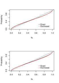
We apply Algorithm 1 to Bayesian logistic regression. Let be a design matrix, let be regression coefficients and be binary response data. For each , where and is the th row of . The likelihood is
We take a prior distribution with the identity matrix. We are interested in the posterior distribution .
The exact posterior can be sampled via standard MCMC. It is also possible to approximate the exact using computationally cheaper Variational Inference (VI) with posterior (Jaakkola and Jordan,, 1997). In this example, we set , and we would like to diagnose the performance of the variational posterior using Algorithm 1. In our example, each entry in the design matrix is sampled independently from . We simulate synthetic -pairs from the generative model , randomly pick one synthetic data point as our observed , and keep the of pairs closest in Euclidean distance to as our training data (this corresponds to a particular choice of in Algorithm 1). Since there is no low dimensional sufficient statistic for this model, we simply use , the dimensional binary response vector, as the summary statistic. We then apply Algorithm 1 using a feed froward neural net with two hidden layers of 80 nodes to estimate the distortion map for each dimension of (recall ), and compare the estimated map to the exact as a function of (the exact map is available for this problem using standard methods).
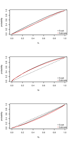
We plot the marginal posteriors and the corresponding exact and fitted distortion maps for the first two dimensions , of the regression parameter in Fig. 1. The fitted distortion map and in the right column accurately recover the exact map. Both and slightly deviate from the identity map, correctly showing that the marginal VI posteriors for and are slightly under-dispersed compared to the exact posterior. This simple example shows our method is able to handle moderately high dimensional () summary statistics .
6 KARATE CLUB NETWORK
In this section we estimate distortion maps measuring the quality of three distinct network model approximations. The data we choose are relatively simple, but happen to illustrate several points neatly. We repeat the analysis on a larger data set in Appendix. The small size of the network data in this example is not an essential point. Conclusions from the larger data set are similar though in some respects less interesting.
The Zachary’s Karate Club network (Zachary,, 1977) is a social network with 34 vertices (representing club members) and 78 undirected edges (representing friendship). The data is available at UCINET IV Datasets. See Fig. 2.
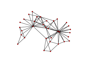
We fit an Exponential Random Graph Model (ERGM) (Robins et al.,, 2007) to these data. Let be the set of all graphs with nodes. Given , let be a -dimensional graphical summary statistic computed on and let be the corresponding ERGM parameter. In our example . In an ERGM, the likelihood of the graph is
| (18) |
where is intractable even for relatively small networks.
Our example approximations come from Caimo and Friel, (2012) and Bouranis et al., (2018). Let be the number of edges in . Following Hunter and Handcock, (2006), let be the number of connected dyads in that have common neighbors, and let equal the number of nodes in that have neighbors. Let
be the geometrically weighted edgewise shared partners (gwesp) statistic and
be the geometrically weighted degree (gwd) statistic. Following Caimo and Friel, (2012) let and , and . Our observation model is given by Eqn 18. The prior distribution for is multivariate normal with and .
The exact is doubly intractable. We consider three approximation schemes yielding different approximations :
- •
- •
-
•
Variational inference (VI) (Tan and Friel,, 2018)
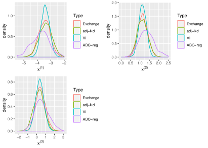
We have ground truth in this example, sampling using an approximate exchange algorithm (Murray et al.,, 2012). This is still approximate but very accurate. For each approximation scheme and dimension , , we fit the distortion map using Algorithm 1 and compare our -diagnostic plot with diagnostic plots obtained using the methods of Prangle et al., (2014) and Talts et al., (2018).
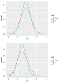
We simulated pairs from the generative model , taking pairs pairs in the top by least Euclidean distance to as our training data. We first report the approximate posteriors themselves. In Fig. 3 (left column) we see that the adj-lkd approach (top row) gives the best approximate posterior for all dimensions. In comparison, the VI approach (bottom row) gives an under-dispersed approximation while the ABC-reg posterior (middle row) is over-dispersed and slightly biased. In a real application we would not have this ground truth.
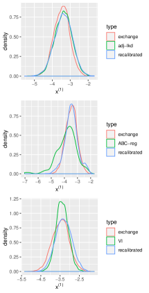
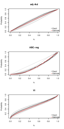
We now run Algorithm 1 using a feed froward neural net with two hidden layers of 80 nodes and estimate for all approximation schemes and dimensions . For brevity we now focus on the distribution of . In Fig. 4 (right column) we show the exact (not available in real applications, but useful to show the method is working) and the fitted for for all three approximation schemes with the corresponding recalibrated posteriors (left column). For all approximation schemes the estimated is close to the exact , and are stable under repeated runs (which were fitted using of the training data). The approximate posterior (with CDF ) matches the true posterior (in the graphs at left in Fig. 4) when is close to an identity map (in the graphs at right in the same figure). The recalibrated posteriors (with CDF ) are closer to the exact, again indicating that our fitted is correct.
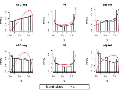
Plots of the distortion density allow direct comparison with the diagnostic histograms of Prangle et al., (2014) and Talts et al., (2018). Adopting those methods in our setting, we average over an open ball centered at containing the top of ’s closest to . We see in Fig. 5, where we plot diagnostics for (top row) and (bottom row), that these diagnostic histograms successfully identify the under-dispersion of VI posteriors (a U-shape in the corresponding histograms (Talts et al.,, 2018) in the middle column). However, the histogram of ABC-reg is reasonably flat for , which seems healthy. This is misleading as the ABC-reg posterior for is in fact over-dispersed at as the -graph in red shows. In contrast, the non-uniformity in the histogram of adj-lkd posterior of (top right) suggests that that approximation is poor, when we see from -graph in red that the approximation is excellent (with ground truth in the top row of Fig. 3 agreeing). The diagnostic histograms of Prangle et al., (2014) and Talts et al., (2018) give both false-positive and false-negative alerts in this example.
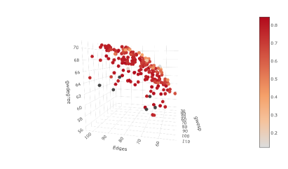
To further illustrate this behavior on the adj-lkd example for , we sampled pairs , so that the ’s are all close to . For each data set , we compute an equal-tail approximate credible set with level for using the adj-lkd posterior. Following Xing et al., (2019) we can ask, what is the true (i.e. “operational”) coverage achieved by this approximate set in the exact posterior? Does the approximate credible set at the data have the stated coverage in the true posterior? The exchange algorithm gives (fairly accurate) samples from the true posterior so the expectation in Eqn. 17 is easily estimated.
In Fig. 6 we plot the points colored by their coverage. Red points points correspond to data where we are getting the right coverage. However there is an orange-colored plane region in the top right part of the plot where is much lower than the nominal level of . The data is located at a red point so the coverage from the adj-lkd approximation is fine (as we would expect from the healthy diagnostics in Fig 5). However when we average we include data where the approximation is poor and reach the wrong conclusion. This illustrates how the quality of approximation can vary over a subset of data space .
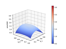
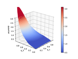
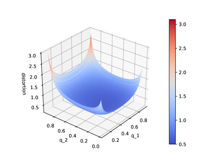
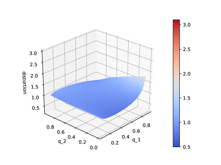
Finally, we estimate and report the bivariate distortion surface for VI and adj-lkd approximations to the posterior for the first two parameters and . From Sec. 3.2, taking and , the distortion surface is
Fig. 7 shows that for the VI posterior, the distortion surface peaks on the boundary and corners of the square, and is below 1 at the center (recall that it is a normalised bivariate probability density). This is the 2-D equivalent of the U shaped diagnostic plots for scalars described in Prangle et al., (2014) and Talts et al., (2018), reflecting the under-dispersed VI posterior approximation. In contrast, the distortion surface of adj-lkd posterior is between and relatively flat over much of the square: there is no evidence here for a problem with the adj-lkd approximation.
7 CONCLUSION
In this paper we give new diagnostic tools for approximate Bayesian inference. The distortion map is a visual diagnostic tool for approximate marginal posteriors, which gives us diagnostic details about the approximation error. It is computationally demanding to estimate. Estimating the distortion map requires sampling synthetic data from the generative model and calling the approximation scheme at each synthetic data point. In contrast to existing methods it checks the quality of approximation at the observed data , instead of estimating “averaged performance” over data space. Much of the code-base (simulation outline, fitting the Beta-density conditioned on -values in a neighborhood of ) carries over from one problem to another, so the user provides simulators for the generative model and the approximate posterior. The approach can be extended from diagnosing univariate marginals to higher dimensions. One interesting direction for future work is to find a way to simulate synthetic data close to while reweighting in a way that yields an unbiased distortion map.
References
- Beaumont, (2010) Beaumont, M. A. (2010). Approximate Bayesian computation in evolution and ecology. Annual review of ecology, evolution, and systematics, 41:379–406.
- Bishop, (1994) Bishop, C. M. (1994). Mixture density networks.
- Bouranis et al., (2017) Bouranis, L., Friel, N., and Maire, F. (2017). Efficient Bayesian inference for exponential random graph models by correcting the pseudo-posterior distribution. Social Networks, 50:98–108.
- Bouranis et al., (2018) Bouranis, L., Friel, N., and Maire, F. (2018). Bayesian model selection for exponential random graph models via adjusted pseudolikelihoods. Journal of Computational and Graphical Statistics, 27(3):516–528.
- Caimo and Friel, (2012) Caimo, A. and Friel, N. (2012). Bergm: Bayesian exponential random graphs in R. arXiv preprint arXiv:1201.2770.
- Cook et al., (2006) Cook, S. R., Gelman, A., and Rubin, D. B. (2006). Validation of software for Bayesian models using posterior quantiles. Journal of Computational and Graphical Statistics, 15(3):675–692.
- El Moselhy and Marzouk, (2012) El Moselhy, T. A. and Marzouk, Y. M. (2012). Bayesian inference with optimal maps. Journal of Computational Physics, 231(23):7815–7850.
- Geweke, (2004) Geweke, J. (2004). Getting it right: Joint distribution tests of posterior simulators. Journal of the American Statistical Association, 99(467):799–804.
- Greenberg et al., (2019) Greenberg, D. S., Nonnenmacher, M., and Macke, J. H. (2019). Automatic Posterior Transformation for Likelihood-Free Inference. arXiv e-prints, page arXiv:1905.07488.
- Hoffman et al., (2013) Hoffman, M. D., Blei, D. M., Wang, C., and Paisley, J. (2013). Stochastic variational inference. The Journal of Machine Learning Research, 14(1):1303–1347.
- Höglund et al., (2006) Höglund, M., Frigyesi, A., and Mitelman, F. (2006). A gene fusion network in human neoplasia. Oncogene, 25(18):2674.
- Hunter and Handcock, (2006) Hunter, D. R. and Handcock, M. S. (2006). Inference in curved exponential family models for networks. Journal of Computational and Graphical Statistics, 15(3):565–583.
- Jaakkola and Jordan, (1997) Jaakkola, T. and Jordan, M. (1997). A variational approach to Bayesian logistic regression models and their extensions. In Sixth International Workshop on Artificial Intelligence and Statistics, volume 82.
- Jordan et al., (1999) Jordan, M. I., Ghahramani, Z., Jaakkola, T. S., and Saul, L. K. (1999). An introduction to variational methods for graphical models. Machine learning, 37(2):183–233.
- Kunegis, (2013) Kunegis, J. (2013). Konect: The Koblenz network collection. In Proceedings of the 22Nd International Conference on World Wide Web, WWW ’13 Companion, pages 1343–1350, New York, NY, USA. ACM.
- Kuśmierczyk et al., (2019) Kuśmierczyk, T., Sakaya, J., and Klami, A. (2019). Variational Bayesian decision-making for continuous utilities. In Advances in Neural Information Processing Systems, pages 6392–6402.
- Lacoste-Julien et al., (2011) Lacoste-Julien, S., Huszár, F., and Ghahramani, Z. (2011). Approximate inference for the loss-calibrated Bayesian. In Proceedings of the Fourteenth International Conference on Artificial Intelligence and Statistics, pages 416–424.
- Lee et al., (2018) Lee, J. E., Nicholls, G. K., Ryder, R. J., et al. (2018). Calibration procedures for approximate Bayesian credible sets. Bayesian Analysis.
- Menendez et al., (2014) Menendez, P., Fan, Y., Garthwaite, P., and Sisson, S. (2014). Simultaneous adjustment of bias and coverage probabilities for confidence intervals. Computational Statistics & Data Analysis, 70:35 – 44.
- Monahan and Boos, (1992) Monahan, J. F. and Boos, D. D. (1992). Proper likelihoods for Bayesian analysis. Biometrika, 79(2):271–278.
- Murray et al., (2012) Murray, I., Ghahramani, Z., and MacKay, D. (2012). MCMC for doubly-intractable distributions. arXiv preprint arXiv:1206.6848.
- Papamakarios and Murray, (2016) Papamakarios, G. and Murray, I. (2016). Fast -free inference of simulation models with Bayesian conditional density estimation. In Advances in Neural Information Processing Systems, pages 1028–1036.
- Prangle et al., (2014) Prangle, D., Blum, M. G., Popovic, G., and Sisson, S. (2014). Diagnostic tools for approximate Bayesian computation using the coverage property. Australian & New Zealand Journal of Statistics, 56(4):309–329.
- Price et al., (2018) Price, L. F., Drovandi, C. C., Lee, A., and Nott, D. J. (2018). Bayesian synthetic likelihood. Journal of Computational and Graphical Statistics, 27(1):1–11.
- Pritchard et al., (1999) Pritchard, J. K., Seielstad, M. T., Perez-Lezaun, A., and Feldman, M. W. (1999). Population growth of human Y chromosomes: A study of Y chromosome microsatellites. Molecular biology and evolution, 16(12):1791–1798.
- Redner et al., (1981) Redner, R. et al. (1981). Note on the consistency of the maximum likelihood estimate for nonidentifiable distributions. The Annals of Statistics, 9(1):225–228.
- Robins et al., (2007) Robins, G., Pattison, P., Kalish, Y., and Lusher, D. (2007). An introduction to exponential random graph (p*) models for social networks. Social networks, 29(2):173–191.
- Rodrigues et al., (2018) Rodrigues, G., Prangle, D., and Sisson, S. A. (2018). Recalibration: A post-processing method for approximate Bayesian computation. Computational Statistics & Data Analysis, 126:53–66.
- Talts et al., (2018) Talts, S., Betancourt, M., Simpson, D., Vehtari, A., and Gelman, A. (2018). Validating Bayesian inference algorithms with simulation-based calibration. arXiv preprint arXiv:1804.06788.
- Tan and Friel, (2018) Tan, L. S. and Friel, N. (2018). Bayesian variational inference for exponential random graph models. arXiv preprint arXiv:1811.04249.
- Wood, (2010) Wood, S. N. (2010). Statistical inference for noisy nonlinear ecological dynamic systems. Nature, 466(7310):1102–1104.
- Xing et al., (2019) Xing, H., Nicholls, G., and Lee, J. (2019). Calibrated approximate Bayesian inference. In Proceedings of the 36th International Conference on Machine Learning, volume 97, pages 6912–6920. PMLR.
- Yao et al., (2018) Yao, Y., Vehtari, A., Simpson, D., and Gelman, A. (2018). Yes, but did it work?: Evaluating variational inference. arXiv preprint arXiv:1802.02538.
- Zachary, (1977) Zachary, W. W. (1977). An information flow model for conflict and fission in small groups. Journal of anthropological research, 33(4):452–473.
Appendix A APPENDIX
A.1 Further discussion
Comparison to ABC
Distortion map estimation shares a number of features with ABC. These include simulation of the generative model and the presence of windowing on data . The window plays different roles, as a marginalising window in ABC recalibration and a conditioning window in distortion map analysis but seems superficially similar. How do the methods compare?
Compared to standard ABC, estimation of a distortion map is fundamentally easier. This is illustrated in Section 5 where ABC is clearly overdispersed but the distortion map is accurately estimated. ABC sets out to approximate the entire joint distribution of the multivariate parameter. For diagnostic purposes the distortion map is targeting scalar or at most bivariate marginals only. The regularisation allowed by the restricted parameterisation of (see the next subsection) is helpful also.
Compared to ABC, estimation of the distortion map has the additional computational cost of a) repeatedly applying the approximation scheme on each synthetic data points (easy when is available in closed form, as is sometimes the case, as in mean-field VI). Existing methods (Talts et al.,, 2018; Rodrigues et al.,, 2018) pay the same price. Another cost is b) fitting the network to the simulated data set (we do this just once). In our experience b) requires much less time than a), so the method presented in this paper works best when the approximation scheme is computationally cheap.
Parameterisation of
In this paper we parameterise as a Beta CDF. This may seem an arbitrary and restrictive choice. However we are partly benefiting from the normalising-flow parameterisation we have set up, as the distortion map is a CDF on . More fundamentally we feel that a parametric restriction or “regularisation” of this sort is the price we pay for estimating a bias (i.e. the distortion of the approximate posterior from the true) without knowing the truth. We are using the Neural Net to regress on a space of (scalar) functions . By restricting this function space we regularise the fit in a helpful way. Other (possibly more flexible) parameterisations of are available. For example, we tried parameterising with a mixture of Beta CDFs (up to 4 components) but found no improvement, just longer run times.
One drawback of our setup is that the single component Beta can be fooled: for example, if the true distortion density was trimodal with peaks at 0.01, 0.5 and 0.99, then the estimated would be close to uniform over [0,1] so our estimated diagnostic would seem to be good when the truth was bad (far from uniform). We can spot this by fitting a mixture of Beta CDFs as a diagnostic.
Consistency and reliability of
We showed consistency of our method in Section 3 under the assumption that the Beta-NN parameterisation is sufficiently expressive. The lemma holds without this assumption but convergence in probability holds for the parameter minimising the KL-divergence. The theorem holds if there exists such that . If this is not the case then the approximation must be good! In this case the MLE converges to , parameterising the identity map, a reasonable diagnostic outcome.
We cannot guarantee for any given that our estimate based on is reliable (it isn’t, as it is only mapping closer to the truth in probability) so some diagnostics are needed to check our diagnostic tool. Section 3.1 lists two obvious validation checks on and we may also vary the number of mixture components in the MDN.
In principle we have access to an unlimited amount of data to learn , if we can efficiently simulate the generative model. However, this type of check can be time consuming, as it requires repeated calls of the approximation scheme for each synthetic data point. This means our method if effective if the computational cost of the evaluating the approximation is manageable.
A.2 Proofs
The following proposition reproduces a result given in Papamakarios and Murray, (2016).
Proposition 1.
Suppose the set in Equation 6 is non-empty. Let independently for . Then converges in probability to
This limit function is maximized at .
Proof.
Our presentation here is very brief as this result is known. We include this proof outline in order to make the meaning of the proposition clear.
By the WLLN,
and the first statement follows as
The second term does not depend on so we maximise the scaled limit of the log-likelihood by minimising the KL-divergence. Since for all iff at each , and is otherwise continuous and positive, the limit function is maximised at whenever this set is non-empty. ∎
The result above shows that the maximum of the limit of the scaled log-likelihood gives the true distortion map. However a proof of consistency must show that the limit of the maximum of the scaled log-likelihood converges in probability to the set of parameter values that express the true distortion map. Standard theory for the MLE does not apply as the true parameter is not identifiable. The corresponding result for the non-identifiable case was given in Redner et al., (1981). The following proof of consistency is based on that paper.
Lemma 1.
Under the conditions of Proposition 1, the estimate is consistent, that is
for every fixed .
Proof.
Let . Let be the quotient topological space defined by taking , choosing a point , and identifying all points in in the original space with the single point in .
We now show (by citing Redner et al., (1981)) that the maximum likelihood estimator converges in to , as . This is not an immediate consequence of standard regularity conditions for the convergence of the MLE, as we do not assume that there is a unique satisfying , so is not identifiable. In fact we can construct cases where has uncountably many elements, so this assumption does not hold. However, the MLE convergence results for a non-identifiable parameter given in Redner et al., (1981) apply. Recall that is the point in the corresponding to the set in the original space . By Theorem 4 of Redner et al., (1981), we have as . All regularity conditions required for Theorem 4 of Redner et al., (1981) can be verified easily.
It then follows from the continuity of (and therefore ) and the continuous mapping theorem that, for each pair ,
and then since we have
∎
Theorem 1.
Under the conditions of Proposition 1 and assuming ,
as for every fixed .
Proof.
so the density of is
Recalling , we have
where we made the change of variables to get from the second to third lines. Taking with we have
By Lemma 1, . The KL-divergence is a continuous mapping, so in probability by the continuous mapping theorem. It follows that the limit as of the quantity on the RHS of the last equality is equal one. ∎
Theorem 1 is a fairly natural consequence of Lemma 1: the procedure is Maximum-Likelihood, satisfies (some rather special) regularity conditions, and is therefore consistent. However we state the result in this form in order to emphasise that Algorithm 1 returns a distortion map that moves closer to , with high probability for all sufficiently large , so that the map contains information about the distorting effects of the approximation, without actually sampling , or even making it possible to sample .
A.3 Gene Fusion network
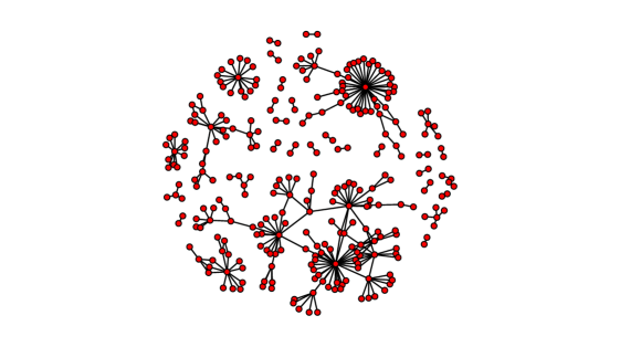
We tried our approach on the larger Gene Fusion network (Höglund et al.,, 2006; Kunegis,, 2013) with 291 nodes and 279 edges. Nodes represent genes and an edge is present if fusion of the two genes is observed during the emergence of cancer. The same ERGM given in Section 6 is used to fit the data.
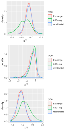
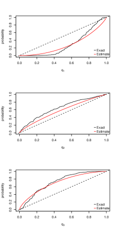
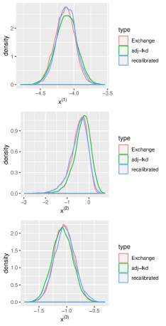
In this example we report the ABC-reg and adj-lkd posteriors only, as the VI posterior behaves in the same way as in the Karate club network example (accurate mode, under-dispersed tails). Again, we report the fitted distortion map and the recalibrated for each for both approximation schemes in Fig. 9 and 10. Fig. 9 and 10 show that estimated distortion maps are close to exact maps for each dimension for both approximation schemes. The estimated distortion map deviates from the identity map when the approximate marginals deviate from the exact substantially, and is close to the identity map when .
As in Section 6 we plot the distortion surfaces for the ABC-reg and adj-lkd posteriors for . In this example there is little interesting bivariate structure as the joint distortion map is essentially the product of the univariate maps. From Fig. 11 we see the distortion surface of the ABC-reg posterior is far from 1, indicating that the ABC-reg approximation of the bivariate marginal posterior is unreliable. The distortion surface of adj-lkd posterior at the data is reasonably close to 1, though somewhat barrel-shaped, reflecting the fact that the approximation to is (fairly slightly) overdispersed.
