Leveraging Machine Learning to Alleviate Hubbard Model Sign Problems

Abstract

Lattice Monte Carlo calculations of interacting systems on non-bipartite lattices exhibit an oscillatory imaginary phase known as the phase or sign problem, even at zero chemical potential. One method to alleviate the sign problem is to analytically continue the integration region of the state variables into the complex plane via holomorphic flow equations. For asymptotically large flow times the state variables approach manifolds of constant imaginary phase known as Lefschetz thimbles. However, flowing such variables and calculating the ensuing Jacobian is a computationally demanding procedure. In this paper we demonstrate that neural networks can be trained to parameterize suitable manifolds for this class of sign problem and drastically reduce the computational cost. We apply our method to the Hubbard model on the triangle and tetrahedron, both of which are non-bipartite. At strong interaction strengths and modest temperatures the tetrahedron suffers from a severe sign problem that cannot be overcome with standard reweighting techniques, while it quickly yields to our method. We benchmark our results with exact calculations and comment on future directions of this work.

I Introduction

Lattice field theories allow for a first-principles construction of non-perturbative interacting quantum field theories. Beyond being a mathematical footing, they provide a computational strategy for solving such systems numerically, typically via Markov-chain Monte Carlo (MCMC). However, for this numerical approach to succeed, a Euclidean field theory requires a real-valued action, providing a positive-definite integration measure. When the action is complex, additional steps must be taken, because the integrand can oscillate wildly. Hence, intricate cancellations are required for numerical estimates to yield accurate results, thereby rendering otherwise successful lattice methods powerless.

This oscillating complex phase problem (“sign problem”) is prevalent in many areas of computational physics that rely on lattice stochastic methods to tackle non-perturbative phenomena.

Lattice quantum chromodynamics (LQCD) calculations at finite baryon chemical potential Splittorff and Verbaarschot (2007); Danzer et al. (2009) suffer from a sign problem, which precludes any numerical investigation of quark matter in dense astrophysical objects such as neutron stars and supernovae Garron and Langfeld (2016); Hsu and Reeb (2010); Goy et al. (2017). Furthermore, including the strong-$\theta$ term Shindler et al. (2015) in the QCD action induces a sign problem as well. Without the development of methods to alleviate the sign problem, one is forced to assume the affected terms are (perturbatively) small  Splittorff and Verbaarschot (2007); Gavai and Gupta (2008); Dragos et al. (2019).

In nuclear lattice effective field theory (NLEFT) Lähde, Timo A. and Meißner, Ulf-G. (2019); Lähde et al. (2015); Elhatisari et al. (2017), where nucleons are degrees of freedom as opposed to quarks, the sign problem prevents lattice MCMC studies of very neutron-rich nuclei. These nuclei, near the neutron drip line, play an important role in today’s nuclear reactors and in the industrial and astrophysical synthesis of heavy elements.

A wide variety of condensed-matter systems, including the doped fermionic Hubbard model, exhibit a rich multi-quasi-particle spectrum (see, for example, Refs. Matsunaga et al. (2011); Deilmann and Rohlfing (2017); Arora et al. (2019); Gaulke et al. (2020)) and comprise tantalizing theoretical systems with commercial relevance. Unfortunately, many of these systems exhibit a sign problem as well. Indeed, the sign problem poses a major stumbling block for MCMC studies in all computational subdisciplines of physics.

Finding a general solution to the phase problem with polynomial scaling in the severity of the problem is NP-hard Troyer and Wiese (2005). However, techniques that take advantage of a particular model’s structure may still be achievable. Therefore, various strategies for alleviating the sign problem have been developed.

The most obvious and widespread of these is reweighting, which we describe in more detail Section II.3. Reweighting can be applied when the sign problem is mild, but can fail spectacularly when the problem is severe, much as perturbation theory fails when the interactions become strong.

Another commonly used strategy is analytic continuation. For example, in QCD one may simulate with purely imaginary baryon chemical potential, removing the complex phase completely (see, for example, Refs. D’Elia and Lombardo (2003); Bellwied et al. (2015); Vovchenko et al. (2017)). Here, the uncertainty lies in the functional form chosen to analytically continue results back to the real axis, which is not known a priori and thus relies on model assumptions. Moreover, analytically continuing Monte Carlo data with uncertainties is no easy task.

Alternatively, Complex Langevin methods do away completely with MCMC and have had various degrees of success (see, for example, Refs. Batrouni et al. (1985); Batrouni (1986); Fukugita et al. (1987); Damgaard and Hüffel (1987), and more recently, Kogut and Sinclair (2019)). Unfortunately, there currently seems to be no consensus on which systems have Langevin methods that are guaranteed to be correct and which do not, though progress has been made in quantifying certain conditions for success Sexty (2014).

Recently, tensor networks White (1992); Verstraete and Cirac (2004); Orus (2014) have shown promise in tackling many-body systems in both one and two dimensions. Their formalism is agnostic to the presence of a chemical potential. First results are available for fermionic systems Corboz and Vidal (2009), such as spinless fermions on the hexagonal lattice Corboz et al. (2018) and the Hubbard model on a square lattice Corboz (2016). It remains to be seen, however, whether such calculations are preferable in terms of precision, scalability, and computational complexity, which also applies to methods that involve direct integration over the group manifold providing polynomial exactness Ammon et al. (2016).

The method we leverage here is related to integration on Lefschetz thimbles. By analytically continuing the integration variables into the complex plane Cristoforetti et al. (2012), one can locate higher-dimensional steepest-descent analogues called Lefschetz thimbles for each critical point. On a thimble the phase is not oscillatory, but constant, up to the residual phase of the Jacobian (which can reintroduce wild oscillations if the thimble is strongly curved Lawrence (2018)). Each thimble has its own constant phase; lattice Monte Carlo on a given thimble can be performed because the phase is global and can be factored out of the integral. A combination of all thimbles which can be reached by holomorphic flow yields the original integral over the real variables, but finding those thimbles (or equivalently, identifying their critical points) is usually difficult.

Early investigations with this method looked at bosonic gauge systems in low dimensions Cristoforetti et al. (2014, 2013); Mukherjee et al. (2013). The Thirring model — non-relativistic fermions with a chemical potential in one dimension — was studied using only one “main” thimble Fujii et al. (2015a, b); Kanazawa and Tanizaki (2015) before yielding to a flow-based method Alexandru et al. (2016a, b); Tanizaki et al. (2016) that approaches a thimble in the limit of long flow times. Moreover, Lefschetz thimbles have found use in higher dimensions, including the 1+1-dimensional Thirring model Alexandru et al. (2017a) and small examples of the doped 2+1-dimensional Hubbard model Ulybyshev et al. (2019a). Gauge symmetry complicates the story but the efficacy of Lefschetz Thimbles in gauge theories is a field of active research Schmidt and Ziesché (2017); Zambello and Di Renzo (2018); Alexandru et al. (2018a); Pawlowski et al. (2020). Beyond Lefschetz thimbles one may find sign-optimized manifolds where even the residual Jacobian phase is handled cleanly Alexandru et al. (2018b, c); Mori et al. (2018a).

The most difficult aspect of attempting a Lefschetz decomposition is that the thimbles’ locations and shapes are not generally known a priori, and that their determination is a complicated and numerically intensive endeavor, especially as systems get larger in higher dimensions. Even when locating critical points is straightforward, deciding whether their thimbles must be included to reproduce the integral of interest is not.

Numerical difficulties abound, as well. For example, the calculation of the Jacobian associated with the transformation from the real plane to these complex manifolds and its determinant can be numerically prohibitive as the system size becomes larger. These issues make an exact Lefschetz Thimble decomposition potentially as difficult as the original sign problem.

Instead one can approximate the thimbles by use of holomorphic flow equations. Rather than completely solving the sign problem, this strategy may merely alleviate it Alexandru et al. (2016a); Nishimura and Shimasaki (2017). Moreover, numerical techniques to estimate the determinant of the Jacobian in an efficient manner fix scaling problems Alexandru et al. (2016c). Still, the determination of these approximate manifolds is less computationally intensive than determining the exact manifolds, especially since they live in high-dimensional spaces.

Machine learning provides a good tool for parameterizing the flowed manifold Alexandru et al. (2017b). We can train a neural network to parameterize an approximate flowed manifold because these manifolds are continuous and smooth. Then, manifolds defined via networks, or learnifolds, can be integrated on to alleviate the sign problem. The gain in speed by use of neural networks can be substantial.

We study the Hubbard model on small non-bipartite lattices which suffer a severe phase problem by incorporating a learnifold into HMC. Even though standard reweighting techniques are completely ineffective, even for some of these small problems, we find that learnifold-HMC allows us to extract correlation functions well, reproducing exact results. In the future we plan to leverage this technique to study fullerenes, such as buckyballs, and anticipate a straightforward application to doped systems as well.

Our paper is organized as follows. In Section II we describe our formalism in detail. In Section III we then describe our algorithm, giving details about how we incorporate machine learning into HMC without compromising the algorithm’s exactness. In Section IV we leverage our method, and show that it reproduces exact results for a number of different observables on some simple systems that may be solved exactly, even when standard reweighting might fail. We point out that there is generally a trade-off between ergodicity and the sign problem. Finally, we give some conclusions in Section V.

II Formalism

In this section we introduce the Hamiltonian used in our studies and discuss the consequences of having a non-bipartite lattice. We then explain reweighting—an exact method for handling complex actions. Finally, we discuss correlation functions and mention the operators we use to construct them.

II.1 The Hamiltonian

We use the Hubbard model in the particle/hole basis Brower et al. (2011); Ulybyshev et al. (2013); Smith and von Smekal (2014); Luu and Lähde (2016); Wynen et al. (2019) to perform simulations. The Hubbard model consists of a tight-binding Hamiltonian,

$$H_{0}=-\sum_{x,y}\left(a_{x,\uparrow}^{\dagger}h_{xy}a_{y,\uparrow}+a_{x,\downarrow}^{\dagger}h_{xy}a_{y,\downarrow}\right)\ ,$$ (1)

where $h_{xy}$ is nonzero if $x$ and $y$ are nearest neighbors, coupled with an onsite interaction of the form

$$H=H_{0}-\frac{U}{2}\sum_{x}\left(n_{x,\uparrow}-n_{x,\downarrow}\right)^{2}\ ,$$ (2)

where the number operator $n_{x,s}\equiv a_{x,s}^{\dagger}a_{x,s}$ counts electrons of spin $s$ at position $x$. We now change to the hole basis for the spin-$\downarrow$ electrons,

$$b_{x,\downarrow}^{\dagger}\equiv a_{x,\downarrow},\quad b_{x,\downarrow}\equiv a_{x,\downarrow}^{\dagger}\ ,$$ (3)

which gives, up to an irrelevant constant,

$$H =-\sum_{x,y}\left(a_{x}^{\dagger}h_{xy}a_{y}-b_{x}^{\dagger}h_{xy}b_{y}\right)+\frac{U}{2}\sum_{x}\rho_{x}^{2}\ ,$$ (4)

$$\rho_{x} =n^{a}_{x}-n^{b}_{x}$$ (5)

where $n^{a}_{x}=a_{x}^{\dagger}a_{x}$ counts the number of (spin-$\uparrow$) particles $n^{b}_{x}=b_{x}^{{\dagger}}b_{x}$ counts the number of spin-$\downarrow$ holes at site $x$; we use the convention of positively-charged particles.

II.2 Non-bipartite lattices

Bipartite graphs are those that admit a two-coloring, such that no vertex has a neighbor of the same color. Examples include the standard square lattice (consisting of two underlying square lattices), the honeycomb lattice (consisting of two underlying triangular lattices), or simply two connected sites. A non-bipartite graph, in contrast, cannot be so colored.

Graphs with odd-length cycles are not bipartite. Examples include fullerene refinements of a 2-sphere, such as the buckyball (C₆₀) or the dodecahedron (C₂₀). In this case the presence of 12 pentagonal faces (required to make the geometry closed) destroys the bipartiteness. The simplest, non-trivial non-bipartite graph is a single triangle, which is small enough for exact diagonalization. The tetrahedron, topologically the complete graph on four vertices, is similarly tractable but not bipartite. The Hubbard model has been studied on non-bipartite quasi-one-dimensional chains Daul and Scalapino (2000); Wang (2005); Rojas et al. (2012) and has been exactly solved on small clusters Schumann (2008) because solutions on such chains and clusters may be taken as input data for many-body methods. The discovery of unusual heavy-fermion behavior of LiV₂O₄ triggered direct studies of the Hubbard model on the pyrochlore lattice with tetrahedral unit cells Hattori and Tsunetsugu (2009) and other extended non-bipartite structures (for example, see Yoshioka et al. (2008a, b); Furukawa et al. (2010)).

As discussed in Ref. Wynen et al. (2019), when the Hubbard model is formulated on a bipartite graph, its formulation as a lattice field theory exhibits special features. Discretizing the Euclidean time $\beta$ into $N_{t}$ timeslices yields a temporal lattice spacing

$$\delta=\frac{\beta}{N_{t}}$$ (6)

and we denote quantities made dimensionless with factors of $\delta$ with a tilde, so that $\tilde{U}=U\delta$. The partition function can be cast into the form of a path integral Brower et al. (2011); Ulybyshev et al. (2013); Smith and von Smekal (2014); Luu and Lähde (2016) yielding

$$\mathcal{Z} =\int\left[\prod_{x,t}\text{d}\phi_{xt}\right]e^{-\beta H[\phi]}=\int\left[\prod_{x,t}\text{d}\phi_{xt}\right]{W[\phi]}$$ (7)

$$W[\phi] =\det\left(M[\phi,h]{M}^{\dagger}[\phi,-h]\right)\exp\left(-\frac{1}{2\tilde{U}}\sum_{x,t}\phi_{xt}^{2}\right)\ ,$$ (8)

where we assume $\tilde{U}>0$ and the fermion matrix is in the exponential discretization (see Ref. Wynen et al. (2019) for a comparison with other discretizations),

$${M[\phi,h]}_{x^{\prime}t^{\prime},xt}=\delta_{x^{\prime},x}\delta_{t^{\prime},t}-{[e^{\tilde{h}}]}_{x^{\prime},x}e^{i\phi_{xt}}\mathcal{B}_{t^{\prime}}\delta_{t^{\prime},t+1},$$ (9)

where $\tilde{h}$ is the dimensionless hopping matrix and $\mathcal{B}_{t}=+1$ for $0<t<N_{t}$ and $\mathcal{B}_{0}=-1$ explicitly encodes anti-periodic temporal boundary conditions.

In the case of bipartite lattices, the particle-hole transformation (3) can be modified to include an additional sign

$$b_{x,\downarrow}^{\dagger} \equiv\mathcal{P}_{x}a_{x,\downarrow} b_{x,\downarrow} \equiv\mathcal{P}_{x}a_{x,\downarrow}^{\dagger}\ ,$$ (10)

where $\mathcal{P}_{x}$ is the parity of the sublattice, so that we perform a site-dependent sign flip—$\mathcal{P}_{x}=+1$ if $x$ is on one sub-lattice, $-1$ if on the other—for holes. This flips the sign of the hopping term in the hole matrix such that the weight becomes

$$W[\phi] =\det\left(M[\phi,h]{M}^{\dagger}[\phi,h]\right)\exp\left(-\frac{1}{2\tilde{U}}\sum_{x,t}\phi_{xt}^{2}\right)$$ (11)

as shown in, for example, Refs. Brower et al. (2011); Ulybyshev et al. (2013); Smith and von Smekal (2014); Luu and Lähde (2016). Since $M{M}^{\dagger}$ is positive-semidefinite, $W$ is real and positive-semi-definite as well. Such systems are thus easily amenable to standard Monte-Carlo simulations.

On non-bipartite lattices the signed particle-hole transformation (10) does not exist, as the bipartitioning fails, so we cannot apply it and the weight (8) is of indefinite sign. The next section describes how Monte-Carlo techniques can nonetheless be applied in this case and discusses the problems such calculations typically face.

We restrict our attention to cases where the hopping matrix $h$ is always just a constant times the graph’s adjacency matrix,

$$h_{xy}=\kappa\;\delta_{\langle x,y\rangle}$$ (12)

though this assumption could be relaxed to model realistic molecules where bond lengths and corresponding hopping strengths vary. In general, the symmetry of the underlying lattice should be considered when determining the Hamiltonian. For example, the regular dodecahedron is vertex- and edge- transitive, so it is natural to assign uniform interaction strengths to every site and uniform hopping strengths along every edge. In contrast, while the truncated icosahedron ($C_{60}$ buckyball) is vertex-transitive and thus every site should have the same interaction strength, it is not edge-transitive: some edges separate two hexagons, while others separate a hexagon from a pentagon and these two different kinds of edges could have different hopping strengths (which physically reflects the fact that the bond lengths differ). In larger fullerenes with $I_{h}$ symmetry there are a wider variety of bond lengths, even between hexagonal faces, because some hexagons are closer to or farther from pentagons; in fullerenes with smaller symmetry groups (such as $C_{70}$, which enjoys a $D_{5h}$ symmetry) we can naturally incorporate its structure by adjusting hopping strengths in $h$ and adjusting $U$ from site to site in a way that respects its symmetry. Since we here are interested in proof-of-principle work we ignore all effects of this kind.

II.3 Reweighting

The expectation value of an observable $\hat{O}$ is given by

$$\langle\hat{O}\rangle=\frac{1}{\mathcal{Z}}\int\mathcal{D}\phi\,\hat{O}[\phi]\ e^{-S[\phi]}$$ (13)

where $S$ is the action, $\phi$ the fields, and $\mathcal{Z}$ the integral without the operator. For the purpose of this discussion we include the fermionic determinants in the action $S$ by taking the log and casting them up into the exponential.

When the action is real-valued we can construct a Monte Carlo method, sampling configurations of the field $\phi$ according to their probability given by the Boltzmann weight $\exp(-S)/\mathcal{Z}$ (“importance sampling”). Generated in such a way, we can estimate the expectation value in (13) by computing the mean of the observable measured separately on each configuration.

When the action is complex-valued the Boltzmann weight is complex as well, and does not directly provide a probability distribution. Reweighting is an exact, straightforward procedure by which we can overcome this difficulty, given sufficient computational resources. Rather than sampling according to the action, one samples according to the real part of the action $S^{R}$ and incorporates the phase associated with the imaginary part of the action $S^{I}$ into each observable, estimating

$$\langle\hat{O}\rangle=\frac{\langle\hat{O}e^{-iS^{I}}\rangle_{R}}{\langle e^{-iS^{I}}\rangle_{R}}\approx\frac{\sum_{j}\hat{O}\left[\phi_{j}\right]e^{-iS^{I}\left[\phi_{j}\right]}}{\sum_{j}e^{-iS^{I}\left[\phi_{j}\right]}}$$ (14)

where $j$ runs over the ensemble and the $R$-subscripted angle brackets indicate an expectation value with respect to the real part of the action only.

If the phase given by the imaginary part of the action is constant or narrowly distributed, this procedure can successfully estimate observables. However, if the phase is widely distributed or, in the worst case, evenly covers the unit circle, the expectation value in the denominator nears zero and reweighting becomes computationally intractable. We call the absolute value of the denominator the statistical power

$$\Sigma=\left|\langle e^{i\theta}\rangle_{R}\right|\ ,\qquad\theta\equiv\arg W\ .$$ (15)

When all configurations have the same imaginary action, $\Sigma=1$ and each configuration is valuable. When $\theta[\phi]$ varies strongly for different field configurations $\phi$, $\Sigma$ is near zero and the configurations tend to cancel; each additional configuration contributes only marginally to the expectation value. Quenching the phase, that is, estimating expectation values by the uncontrolled approximation $\langle\hat{O}\rangle\simeq\langle\hat{O}\rangle_{R}$, can lead to a dramatic distortion of observables.

II.4 Correlation Functions

Two-point correlation functions between two operators $\hat{O}_{x}$ and ${\hat{O}}^{\dagger}_{y}$ at different times and sites $x$, $y$

$$C_{xy}(\tau)=\frac{1}{\mathcal{Z}}\text{tr}\left[e^{-\beta H}\frac{1}{N_{t}}\sum_{t}\hat{O}_{x}(t+\tau){\hat{O}}^{\dagger}_{y}(t)\right]=\frac{1}{N_{t}}\sum_{t}\left\langle\hat{O}_{x}(t+\tau){\hat{O}}^{\dagger}_{y}(t)\right\rangle$$ (16)

can be computed as a function of temporal separation by solving for propagators on each configuration and tying them together in the required Wick contractions. They admit spectral decompositions

$$C_{xy}(\tau) =\frac{1}{\mathcal{Z}}\text{tr}\left[e^{-\beta H}\frac{1}{N_{t}}\sum_{t}\hat{O}_{x}(t+\tau){\hat{O}}^{\dagger}_{y}(t)\right]=\frac{1}{N_{t}}\sum_{t}\frac{1}{\mathcal{Z}}\text{tr}\left[e^{-\beta H}\ e^{+H(t+\tau)}\hat{O}_{x}e^{-H(t+\tau)}\ e^{+Ht}{\hat{O}}^{\dagger}_{y}e^{-Ht}\right]$$

$$=\frac{1}{\mathcal{Z}}\text{tr}\left[e^{-(\beta-\tau)H}\ \hat{O}_{x}\ e^{+H(t+\tau)}\ e^{-Ht}{\hat{O}}^{\dagger}_{y}\right]=\frac{1}{\sum_{a}e^{-E_{a}\beta}}\sum_{bc}e^{-E_{b}\beta}e^{-(E_{c}-E_{b})\tau}z_{axb}z_{b{y}^{\dagger}a}$$ (17)

where we moved to the Heisenberg picture and inserted resolutions of the identity in the energy eigenbasis and defined the overlap factors

$$z_{axb} =\left\langle a\middle|\hat{O}_{x}\middle|b\right\rangle z_{b{y}^{\dagger}a} =\left\langle b\middle|{\hat{O}}^{\dagger}_{y}\middle|a\right\rangle=z_{ayb}^{*}$$ (18)

where $a$ and $b$ label energy eigenstates. In the low temperature limit $\beta\rightarrow\infty$ the sum is dominated by the lowest energy state; otherwise thermal artifacts may be seen. In the low temperature and late-(euclidean-)time limit $\tau\rightarrow\infty$, the correlator’s $\tau$ dependence gives the energy gap between the ground and the first excited state (with the observable’s quantum numbers), as all the heavier states decay more quickly.

Hence, we can extract the single-particle/single-hole spectrum by e.g. setting ${\hat{O}}^{\dagger}_{x}={a}^{\dagger}_{x}$. $C_{xy}(\tau)$ is quadratic in the volume. However, after diagonalization one obtains only $O(V)$ single-particle eigenfunctions. For the small lattices we study here, it suffices to project $x$ and $y$ to the same irreducible representation of the lattice symmetry in order to diagonalize $C$.

We can also calculate correlation functions between composite operators at additional computational expense. The composite operators we consider are the number operators $n^{a}_{x}$ and $n^{b}_{x}$, their sum the total number operator $n_{x}$, their difference the charge operator $\rho_{x}$, spin raising and lowering operators $S^{\pm}_{x}$, and the spin operators $S^{i}_{x}$ (where $i$ runs over all 3 spatial directions); we also consider the two doubly-charged local bilinears. In Appendix A we detail the operators, the correlation functions we measure and how to construct conserved quantities from them.

III Algorithm

We gave an extensive overview of our application of Hybrid Monte Carlo (HMC) to the Hubbard model in Ref. Wynen et al. (2019). In all our reweighting-only examples we run HMC in a standard way, performing the Metropolis accept-reject step according to the real part of the action. In the rest of this section we detail how we incorporate learnifolds into HMC.

In Section III.1 we provide a summary of why integrating over a manifold given by holomorphic flow is advantageous for reducing the sign problem. Then in Section III.2 we show how we use machine learning to quickly compute the learnifold, over which we will integrate. Afterwards we explain how to incorporate the learnifold into HMC and, finally, comment on our update scheme’s ergodicity in Section III.3.

III.1 Holomorphic Flow

Holomorphic flow is a generalization of the steepest descent method to multi-dimensional complex space. Given a holomorphic functional, in our case the action $S$, of the $N$-dimensional complex $\phi$, the flow equations are

$$\frac{\text{d}\phi}{\text{d}\tau_{f}}=\pm\left(\frac{\partial S[\phi]}{\partial\phi}\right)^{*}\ ,$$ (19)

where $\tau_{f}$ is the flow time. A minus sign indicates downward flow, while a plus sign upward flow. Splitting the components $\phi_{i}=\phi^{R}_{i}+i\phi^{I}_{i}$ and the action $S[\phi]=S^{R}[\phi]+iS^{I}[\phi]$ into their real and imaginary parts, yields

$$\frac{\text{d}\phi^{R}}{\text{d}\tau_{f}} =\pm\frac{\partial S^{R}}{\partial\phi^{R}_{i}}=\pm\frac{\partial S^{I}}{\partial\phi^{I}_{i}}$$ (20)

$$\frac{\text{d}\phi^{I}}{\text{d}\tau_{f}} =\pm\frac{\partial S^{R}}{\partial\phi^{I}_{i}}=\mp\frac{\partial S^{I}}{\partial\phi^{R}_{i}}\ ,$$ (21)

which are the Cauchy-Riemann equations. The equations containing $S^{R}$ essentially implement the gradient flow, whereas the other equations are Hamilton’s equations for the imaginary part of the action. That is, $S^{I}$ remains a constant of motion during the flow. It is easily seen that downward holomorphic flow is the generalization of gradient flow, or steepest descent, for real fields.

The critical points $\hat{\phi}_{cr}$ of $S[\phi]$ are vectors of complex numbers and satisfy

$$\frac{\partial S[\phi]}{\partial\phi}\bigg{|}_{\hat{\phi}_{cr}}=0\ .$$ (22)

The $\hat{\phi}_{cr}$ are saddle points; the associated Lefschetz thimble is the manifold in $\mathds{C}^{N}$ which flows to the given critical point under downward flow, while the dual thimble flows to the critical point under upward flow. Models with many variables have many critical points and associated thimbles that must be integrated over to produce the same result as the integral on the real manifold.

Flowing the integration region of $\phi\in\mathds{R}^{N}$ to the manifold(s) $\hat{\phi}$ eliminates the sign problem since $S^{I}$ is constant on each manifold. Because there are no poles in the integration kernel, Cauchy’s integral formula guarantees that the integral over the thimbles $\hat{\phi}\in\mathds{C}^{N}$ will be exactly equal to the original integral over $\phi\in\mathds{R}^{N}$,

$$\int\mathcal{D}\phi\,e^{-S[\phi]}=\sum_{\sigma}e^{-iS^{I}[\hat{\phi}_{cr,\sigma}]}\int\mathcal{D}\hat{\phi}_{\sigma}\,e^{-S^{R}[\hat{\phi}_{\sigma}]}\ ,$$ (23)

where $\sigma$ runs over included thimbles and $\hat{\phi}_{cr,\sigma}$ is the critical point associated with this thimble. The number of thimbles, their critical points, and their relative weights depend on the lattice action and the original integration region (typically $\mathds{R}^{N}$). Not all the thimbles in $\mathds{C}^{N}$ are included in the sum; only those that are required to preserve the integral’s homology class.

Thimbles do not cross each other, but are connected at places where the action diverges so that the integration kernel vanishes. The gaussian part of the action diverges when $|\hat{\phi}|\to\infty$; the fermionic part of the action diverges when $\det(M[\hat{\phi}]M[-\hat{\phi}])=0$. We call these zero-weight places in the complex space neverland, as they never appear in an importance-sampling scheme.

Because the locations of the needed critical points and their associated thimbles are not known a priori, their determination requires extensive numerical resources; an analytic determination would amount to a solution of the lattice model. Instead we follow Alexandru, Basar, and Bedaque Alexandru et al. (2016b) and use the fact that the thimbles are fixed points of the flow to our advantage: we flow only a modest amount to get an integration manifold that approaches the set of relevant thimbles, not solving the sign problem entirely but alleviating it to the point where standard reweighting techniques are sufficient to address any remaining sign problem.

To ensure our method remains exact, it is important that our ultimate integration manifold is in the same homology class as the original. Because the holomorphic flow preserves the homology class, the manifold resulting from any finite flow time is in the right class. Moreover, because the flow’s fixed points are thimbles, a finite-flow manifold approaches those thimbles that contribute to the integral Alexandru et al. (2016b); we need not analytically decide which thimbles to include—the flow discovers this automatically.

One point on the original manifold flows to a thimble’s critical point, and only a vanishing neighborhood around that point flows to the rest of the thimble—most of the original manifold flows to neverland—the place where thimbles meet and vanish in the integration kernel, typically due to zeros of the fermion determinant. These zeros act as attractors, and most configurations flow to these zeros after a finite amount of flow time Kanazawa and Tanizaki (2015); Alexandru et al. (2016b); Mori et al. (2018b). Because the thimbles must meet at these zeros, attempting an update method like HMC on the thimbles themselves in a naive way will be obstructed by these zeros, causing an ergodicity problem. However, by restricting ourselves to modest flow times, we can ensure that the manifold will not touch these zeros. We provide some visual evidence of ergodicity in Section IV.1.1 and reproduce a wide range of exactly-known correlation functions. So, deciding how much to flow is a balancing act—one hopes to flow enough that the sign problem is alleviated but not so much that an ergodicity problem emerges.

Any transformation of integration variables, including the one provided by the flow, comes with an associated Jacobian, and this Jacobian must be included in the Monte Carlo weight (or incorporated by reweighting) for a correct method. There are flow equations for the Jacobian as well Alexandru et al. (2016a),

$$\frac{\text{d}J}{\text{d}\tau_{f}}(t)=\left[H[\phi(t)]J(t)\right]^{*}\ ,$$ (24)

where $H$ is the Hessian,

$$H_{ij}[\phi]\equiv\left.\frac{\partial^{2}S}{\partial\phi_{i}\partial\phi_{j}}\right|_{\phi}=\left.\left(\text{tr}\left[M^{-1}(\partial_{i}M)M^{-1}(\partial_{j}M)\right]-\text{tr}\left[M^{-1}\partial_{i}\partial_{j}M\right]\right)\right|_{+\kappa,+\phi}+\left(\kappa,\phi\rightarrow-\kappa,-\phi\right)+\frac{\delta_{ij}}{\tilde{U}}\ .$$ (25)

Flowing the Jacobian is the most time-consuming aspect of this calculation and thus the reason for considering neural networks, as we discuss in the following section.

To perform the numerical integration of the flow equations (19), and when necessary of the Jacobian (24), we use a 4^th order adaptive Runge-Kutta method. Because the flow preserves the imaginary part of the action, we monitor the latter during the numerical integration and adjust the integration stepsize to keep deviations within a prescribed tolerance.

III.2 Networks

III.2.1 Architecture

We use feed-forward neural networks of dense layers to tackle the sign-problem. Like Refs. Alexandru et al. (2017b); Mori et al. (2018a) these networks produce the imaginary part of a field configuration from the real part and keep the latter fixed. The transformation into complex space is thus

$$\tilde{\phi}=\phi+i\ \text{NN}(\phi),$$ (26)

where NN is the neural network. In addition to the ability of the network to avoid dealing with complex numbers directly, Ref. Alexandru et al. (2017b) points out two advantages this formulation enjoys over $\tilde{\phi}=\text{NN}(\phi)$: it might ameliorate the ergodicity problem that flowing can induce (for an enlightening discussion and illustration see their Figure 2); and it tends to yield a more stable Jacobian (Figure 3 of Ref. Alexandru et al. (2017b)).

We encode $\phi$ as a spacetime vector and use neural networks with a single hidden layer, consisting of twice the number of neurons than the input and output layers. The hidden layer has a Softplus activation function

$$\text{Softplus}(x)=\log(1+\exp(x)),$$ (27)

and the output layer has none. We found this to be sufficient for all cases we tested. Wider or deeper networks as well as convolutional layers or different activation functions did not yield significantly better results. It remains to be seen whether this setup scales to larger spatial lattices.

Neural networks of the chosen architecture can be evaluated very efficiently, which is, unfortunately, only half of the story. We also need to compute the Jacobian determinant for the change of variables, which will appear in the transformed integral (35). Given (26), it is

$$\det J[\phi]=\det\bigg{(}\mathds{1}+i\frac{\partial\text{NN}_{i}(\phi)}{\partial\phi_{j}}\bigg{)}\ .$$ (28)

This operation is $\mathcal{O}\big{(}{(N_{s}N_{t})}^{3}\big{)}$ (cubic in the spacetime volume), because both the determinant and matrix multiplications in the derivative need to be performed with a general algorithm for dense matrices. No speedup seems possible for vanilla dense networks as the weight matrices are unconstrained. We still find our network-based transformation to significantly outperform flow-based transformations in terms of run time, however. But this approach does not scale to larger lattices. It is possible to improve on the scaling by estimating the Jacobian as in Ref. Alexandru et al. (2017b) which uses a different network that produces only one component of $\tilde{\phi}_{I}$ at a time. Alternatively, one can use coupling layers which were designed to have simple Jacobians. This requires complex valued networks in our case, however, as described in Appendix B.

We implemented the neural networks and training procedures using PyTorch Paszke et al. (2019) and used Isle Wynen and Berkowitz (2020) to implement Monte-Carlo for the Hubbard model. Section III.3 describes the HMC scheme we used to accommodate neural networks.

III.2.2 Training procedure

We train our models using a supervised approach. To that end, we generate random real configurations $\phi$ and flow them upward according to Eq. (19) for a fixed flow time to $\hat{\phi}$. It is non-trivial how to generate useful data and we provide explicit details on our approach in Section III.2.3. Once the data is generated, we use $\text{Re}\,\hat{\phi}$ as inputs and $\text{Im}\,\hat{\phi}$ as target outputs to train the networks. We do so by using the Adam algorithm Kingma and Ba (2014) to minimise a smooth L1 loss

$$\text{loss}(x,y)=\frac{1}{n}\sum_{i}^{n}\begin{cases}{(x_{i}-y_{i})}^{2}/2,&\text{for}\left|x_{i}-y_{i}\right|<1\\ \left|x_{i}-y_{i}\right|-1/2,&\text{otherwise}\end{cases}$$ (29)

as defined in PyTorch Paszke et al. (2019).

We know our action has exact symmetries (see Ref. Wynen et al. (2019) for a listing), comprising transforms $T$ that change field configurations but leave the action invariant, $S[T\phi]=S[\phi]$. A uniformly-flowed manifold exhibits many of those symmetries, the most obvious being the temporal and spatial translation symmetries. Naturally it is desirable that our neural networks preserve as many of these symmetries as possible.

Ref. Alexandru et al. (2017b) accomplishes this by training a network that takes a whole spacetime vector and produces only the flowed configuration at the spacetime origin and using translational invariance to construct the other vector elements. This technique suffers a number of constraints, most notably, it requires full translational invariance of the lattice. This is not the case for many interesting non-bipartite lattices, however, as they are not necessarily vertex-transitive. In such a case a network with a single output is not enough because spatial symmetries cannot take every element to every other.

As described above, our neural networks produce a full spacetime vector as output and we encode symmetries by augmenting the training data. One symmetry that all lattices have is temporal translational invariance. We thus train our networks not only on the configurations generated according to Section III.2.3 but also on all possible temporal shifts of the input and target output configurations. This effectively increases the size of the data set by a factor of $N_{t}$. The lattices considered in this work, triangle and tetrahedron, are vertex-transitive and we tried augmenting the training data by all possible spatial permutations but did not find an improvement. Adding temporal translations proves very useful for increasing model quality, however.

Every model was trained on minibatches of size 16 drawn from 1000 random configurations plus temporal translations. The only exception is the tetrahedron with $N_{t}=32$ whose model was trained with 4000 configurations. We found this larger number necessary to train the network well. For larger $N_{t}$, 1000 configurations were enough for the tetrahedron which might be due to the higher number of added configurations from augmentation by temporal translations.

III.2.3 Training: Data

Several different methods have been used to generate training data. Ref. Mori et al. (2018a) uses HMC with a partially trained model to generate data for the next iteration of training. This is expensive as new configurations have to be generated every time model hyperparameters are changed. Because it is self-reinforcing, it is possible that such an approach can find and remain in a local minimum or overfit a part of the phase space.

Ref. Alexandru et al. (2017b) uses HMC without a neural network to generate training data before fitting a model. In order to achieve large phase space coverage, several MC ensembles with different temperatures were generated. This approach needs to generate data only once per parameter set and therefore allows for faster tuning of hyperparameters. It is still susceptible to autocorrelations, though, meaning that a large number of configurations might be needed for sufficient phase space coverage.

One of the goals of this work is to simplify the generation of training data in order to develop a more scalable approach.

One thimble of the Hubbard model on non-bipartite lattices is easy to find — the image of $\text{Re}\ \phi\equiv 0$ under the flow. It connects to a critical point $\hat{\phi}_{\text{cr}}\equiv ic$ for some $U$, $\beta$, and $N_{t}$ dependent value $c<0$. In concordance with literature, we call this the “main” thimble. There is an ongoing discussion whether a single thimble Ref. Cristoforetti et al. (2012) or multiple thimbles are require to solve the integral Alexandru et al. (2016b, a); Kanazawa and Tanizaki (2015); Tanizaki et al. (2016). To be on the safe side, we, therefore, identified additional thimbles, all with spacetime-constant $\hat{\phi}_{\text{cr}}=z\in\mathds{C}$, but close to the main thimble. Figure 1 shows the critical points for a sample system.

We produced training data by first generating random field configurations close to the critical points that we found and then flowing them for a short, fixed flow time. In order to reduce the required flow time, we sampled the initial configurations on the plane tangent to the main thimble in the critical point ($\phi=\phi^{R}+ic$); this is referred to as the “tangent plane” from now on. Models trained on these configurations for a triangle lattice can sometimes reduce the sign problem but are prone to producing learnifolds with a wrong homology class. This problem becomes worse the larger $N_{t}$ is and we did not obtain any successful models for the tetrahedron. The reason is the following.

Empirically, we found that the dependence of the typical set of the probability distribution $W$ on the vector norm $\left|\text{Re}\,\phi\right|$ is almost the same as that of a normal distribution. In high dimensions, the typical set of a gaussian, that is the region of phase space that contains most of the probability, is a thin hyperspherical shell around the origin. Importance sampling, by definition, generates fields that lie in the typical set. We can thus use HMC to visualize the set, an example is shown in orange in Figure 1. The critical points of all thimbles that we used are shown as crosses in the figure. It can be seen that those points are close to the origin and far away from the typical set. Therefore, it should not be surprising that neural networks trained on fields near the critical points do not generalize well to the typical set and yield poor performance of HMC.

Figure 1: Distributions of configurations used for training data (blue-shaded region) and an ensemble produced via HMC with a neural network (orange-shaded region) trained on this data. The system is a triangle with $N_{t}=32$, $\kappa\beta=6$, and $U/\kappa=3$. The distributions were estimated from $10^{5}$ training and $10^{6}$ HMC configurations. The black crosses mark critical points of spacetime-constant $\phi$.

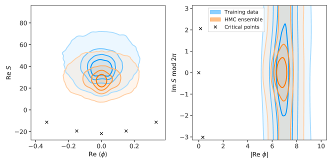
The approach used in this work is motivated by the dominance of the gaussian part of the action. We draw $\text{Re}\ \phi$ randomly from a gaussian and set $\text{Im}\ \phi$ to be on the tangent plane of the main critical point. These $\phi$ are then flowed upwards. This method has two numerical parameters that need to be tuned. One is the width of the gaussian $\sigma$, the other is the flow time. Plots like Figure 1 provide good estimates for the quality of training data. The better the overlap between training data and HMC in these projections the better the neural network performs. Fortunately, the distributions explored by HMC with and without neural networks are largely identical in these projections for well trained models. It is thus sufficient to sample configurations on the real plane in order to estimate the HMC distribution — even though the figure shows an ensemble generated with a network. The overlap shown in the figure, while not perfect, is enough and the figure shows data from a successful run with reduced sign problem shown in more detail below.

Samples drawn from a normal distribution of fixed width $\sigma=\sqrt{\tilde{U}}$ have poor overlap in figures like Figure 1. To remedy this, we draw the width of every sample randomly from a uniform distribution $\mathcal{U}$

$$\sigma\sim\mathcal{U}\Big{(}\sqrt{\tilde{U}}/x,\;\sqrt{\tilde{U}}\,\Big{)}$$ (30)

and then draw $\phi$ from a normal distribution $\mathcal{N}$ with that width: $\text{Re}\ \phi\sim\mathcal{N}(0,\sigma)$. The factor $x$ is chosen such that the overlap of HMC ensemble and training data is maximized.

Similarly, the other parameter, the flow time $\tau_{f}$, needs to be chosen such that plots like Figure 1 show good overlap. Additionally, one needs to strike a balance between reducing the sign problem and avoiding ergodicity problems as described in Section III.1. It is easy to show that for spacetime-constant $\phi$ the gradient of the action is invariant under simultaneous $N_{t}\to\alpha N_{t}$ and $\phi\to\phi/\alpha$. The starting position for flow, which is on the main tangent plane, has, therefore, the same $N_{t}$ dependence. We use this scaling for the flow time as well and choose it to be

$$\tau_{f}^{\text{max}}=0.1\times 16/N_{t}$$ (31)

in all cases. As with $\sigma$, this scaling was found purely based on numerical experiments.

We found significant improvements in both the time required to make training data and the performance of the final neural networks by not requiring a fixed flow time. When using holomorphic flow directly within MC, it is necessary to fix the flow time in order for all configurations to be on the same manifold. In our case, the neural network ensures this regardless of how the training data was created. Many configurations generated from a gaussian quickly flow into neverland and flowing becomes numerically unstable. It is thus impossible to reach the targeted flow time. Instead of discarding these configurations, we monitor the integrator for stability, abort early in such a case, and add the last configuration that could be reached in a stable way to the set of training data. However, it does not make sense to use configurations that could only be flowed for very short times as those provide little information to the neural network. We thus require a minimum flow time of

$$\tau_{f}^{\text{min}}=0.04\times 16/N_{t}$$ (32)

for all training configurations.

III.3 HMC

Rather than implementing HMC on the curved manifold of Lefschetz thimbles defined through holomorphic flow Fukuma et al. (2019) or learnifolds, we pull back to the real plane before performing molecular dynamics, as will now be explained.

Given a transformation into complex space as implemented by holomorphic flow or neural networks, we need to incorporate that transformation into Hybrid Monte-Carlo. Let

$$f:\mathds{R}^{N}\to\mathds{C}^{N},\phi\mapsto\tilde{\phi}\qquad\text{and}\quad J_{ij}[\phi]\equiv\frac{\partial f_{i}(\phi)}{\partial\phi_{j}}\ ,$$ (33)

with $\mathcal{M}\equiv f(\mathds{R}^{N})$ the image of $f$. We want to calculate observables by integrating over the manifold $\mathcal{M}$ because with suitably chosen $f$ the sign problem is alleviated on that manifold. Since $\mathcal{M}$ is in the same homology class as $\mathds{R}^{N}$ and the integrand is regular in $\phi$, by Cauchy’s theorem the expectation value of an observable $\hat{O}$ is

$$\langle\hat{O}\rangle=\frac{1}{\mathcal{Z}_{\mathds{R}^{N}}}\int_{\mathds{R}^{N}}\mathcal{D}\phi\,\hat{O}[\phi]e^{-S[\phi]}=\frac{1}{\mathcal{Z}_{\mathcal{M}}}\int_{\mathcal{M}}\mathcal{D}\tilde{\phi}\,\hat{O}[\tilde{\phi}]e^{-S[\tilde{\phi}]}\ .$$ (34)

We do not know $\mathcal{M}$, however, and can thus not evaluate the integral on the right hand side directly. Instead, we parameterize it using $f$. That is, we perform a transformation of integration variables:

$$\frac{1}{\mathcal{Z}_{\mathcal{M}}}\int_{\mathcal{M}}\mathcal{D}\tilde{\phi}\,\hat{O}[\tilde{\phi}]e^{-S[\tilde{\phi}]} =\frac{1}{\mathcal{Z}_{\mathds{R}^{N}}}\int_{\mathds{R}^{N}}\mathcal{D}\phi\,\hat{O}[\tilde{\phi}(\phi)]e^{-S[\tilde{\phi}(\phi)]}\det J[\phi]\ .$$ (35)

Now define the effective action as

$$S_{\text{eff}}[\tilde{\phi}(\phi)]\equiv S[\tilde{\phi}(\phi)]-\log\det J[\phi]\ .$$ (36)

We can estimate the integral stochastically by generating an ensemble $\{\phi\sim\exp(-\text{Re}S_{\text{eff}}[\tilde{\phi}(\phi)])\}$, where we use the real part of $S_{\text{eff}}$ as per the reweighting procedure described in Sec. II.3. This effectively produces an ensemble $\{\tilde{\phi}=f(\phi)\sim\exp(-\text{Re}S[\tilde{\phi}])\}$ on which the observables $\hat{O}$ can be measured.

We use HMC to generate the ensembles. To this end, we augment the integral by multiplying with a one in the form of an integral over the artificial conjugate momentum $p$ such that

$$\langle\hat{O}\rangle=\frac{1}{\mathcal{Z}}\int\mathcal{D}\phi\mathcal{D}p\,\hat{O}[\tilde{\phi}(\phi)]e^{-i\text{Im}S_{\text{eff}}[\tilde{\phi}(\phi)]}e^{-H[p,\tilde{\phi}(\phi)]},\quad H[p,\tilde{\phi}(\phi)]\equiv\frac{p^{2}}{2}+\text{Re}S_{\text{eff}}[\tilde{\phi}(\phi)]\ .$$ (37)

All integrals are to be understood as integrating over $\mathds{R}^{N}$ from now on. We can encapsulate all dependencies on $f$ in a modified HMC algorithm such that it produces configurations on $\mathcal{M}$ suitable for measurements. The following summarizes the algorithm:

complexified HMC  in: $\tilde{\phi}$ out: $\tilde{\phi}^{\prime}$
$\phi\leftarrow f^{-1}(\tilde{\phi})$	# transform to $\mathds{R}^{N}$
$p\leftarrow\mathcal{N}_{0,1}$	# draw random momentum
$\psi^{\prime},\,p^{\prime}\leftarrow\textsf{molecular\_dynamics}(\phi,\,p)$	# generate candidate on $\mathds{R}^{N}$
$\tilde{\psi}^{\prime}\leftarrow f(\psi^{\prime})$	# transform to $\mathcal{M}$
$\tilde{\phi}^{\prime}\leftarrow\textsf{accept\_reject}(H[p^{\prime},\,\tilde{\psi}^{\prime}],H[p,\,\tilde{\phi}])$	# pick new field

A new configuration is obtained from an old one by first transforming the old complex field $\tilde{\phi}$ to the real plane where it is then updated using molecular dynamics (MD), or any other suitable updating scheme, such as the large jumps explained in Ref. Wynen et al. (2019). The new candidate field $\psi$ is then transformed to $\mathcal{M}$ where it is accepted or rejected using a Metropolis-Hastings step.

It remains to prove that this algorithm produces a Markov Chain. For this, we adopt the picture that we are producing real fields $\{\phi\sim\exp(-\text{Re}S_{\text{eff}}[\tilde{\phi}(\phi)])\}$. Such a proof is equivalent to showing that $\{\tilde{\phi}\}$ is a Markov Chain sampled from $\exp(-\text{Re}S[\tilde{\phi}])$. We do so by first proving detailed balance

$$\mathds{P}(\phi)\mathds{P}(\phi^{\prime}|\phi)=\mathds{P}(\phi^{\prime})\mathds{P}(\phi|\phi^{\prime})$$ (38)

with (ignoring normalization factors)

$$\mathds{P}(\phi) =e^{-\text{Re}S_{\text{eff}}[\tilde{\phi}(\phi)]}$$ (39)

$$\mathds{P}(\phi^{\prime}|\phi) =\int\mathcal{D}p^{\prime}\mathcal{D}p\,e^{-p^{2}/2}\mathds{P}_{\text{MD}}(p^{\prime},\phi^{\prime}|p,\phi)\mathds{P}_{\text{a/r}}(p^{\prime},\tilde{\phi}(\phi^{\prime})|p,\tilde{\phi}(\phi))\ .$$ (40)

$\mathds{P}_{\text{MD}}$ and $e^{-p^{2}/2}$ are the same molecular dynamics and gaussian probabilities as in standard HMC. The prior $\mathds{P}(\phi)$ and accept/reject

$$\mathds{P}_{\text{a/r}}(p^{\prime},\tilde{\phi}(\phi^{\prime})|p,\tilde{\phi}(\phi))=\min\left(1,\;\frac{\exp\left(-\frac{p^{\prime 2}}{2}-\text{Re}S_{\text{eff}}[\tilde{\phi}(\phi^{\prime})]\right)}{\exp\left(-\frac{p^{2}}{2}-\text{Re}S_{\text{eff}}[\tilde{\phi}(\phi)]\right)}\right)$$ (41)

probabilities use the effective action which encapsulates $\tilde{\phi}$. Thus the proof of detailed balance (38) proceeds as usual for HMC. The only ingredient missing to fully prove correctness of our algorithm is a proof of ergodicity. Such a proof is generally not available even for standard HMC. We thus rely on a posteriori analyses to verify ergodicity. Certainly with a long flow time we expect many configurations to flow to neverland, creating large zero-probability regions that separate important islands of configurations. However, if we only flow a little, few if any configurations flow to neverland and the manifold of integration is not partitioned. Our ability to reproduce exact results in Section IV suggests that our method successfully explores fields whose images are near different thimbles. A well trained network inherits these properties from the flowed manifold of its training data.

IV Results

To demonstrate the efficacy of the neural network methods we will explore small lattices, leaving larger lattices for future work. In particular, we here consider the triangle and tetrahedron, both maximally connected and therefore, where we expect the worst sign problem.

IV.1 The Triangle

Three spatial sites is the smallest nontrivial non-bipartite graph we might study—the two-site problem is bipartite and the one-site problem has no hopping at all. We studied those problems extensively using the lattice methods applied here in Ref. Wynen et al. (2019).

Figure 2: The entire spectrum of the Hubbard model on a triangle as a function of $U/\kappa$, changing from 0 to 5 in 20 equal steps, with colors corresponding to different $U/\kappa$. Energy eigenfunctions carry $Q$, $S$, $S_{z}$ and $L_{z}$ quantum numbers; each panel projects the five-dimensional space onto one quantum number and the energy. Each $U/\kappa$ is slightly offset, so that each point in the spectrum for $U/\kappa=0$ is to the left of that point’s quantum numbers, while $U/\kappa=5$ is to the right. One translucent point is plotted per state; more opaque circles correspond to more highly degenerate states. The ground-state manifold qualitatively changes at $U^{\triangle}/\kappa=3.61775\ldots$, shown in a deep blue.

The hopping matrix is given by

$$h=\kappa\left(\begin{array}[]{ccc}0&1&1\\ 1&0&1\\ 1&1&0\end{array}\right),$$ (42)

and the Hamiltonian has $D_{3}$ dihedral symmetry. When diagonalized, the hopping matrix reveals one spatially uniform (trivial) irrep with eigenvalue $2\kappa$ and a dimension-two irrep with eigenvalue $-\kappa$.

The unitary site permutation operator $P$

$$P\;a_{x}\;{P}^{\dagger} =a_{x+1} P\;b_{x}\;{P}^{\dagger} =b_{x+1}$$

$$P\;{a}^{\dagger}_{x}\;{P}^{\dagger} ={a}^{\dagger}_{x+1} P\;{b}^{\dagger}_{x}\;{P}^{\dagger} ={b}^{\dagger}_{x+1}$$ (43)

rotates the sites into one another (the indices on the ladder operators are understood mod 3). $P$ trivially commutes with the potential and nontrivially with the hopping (1).

The three irreducible single-particle destruction operators are

$$\hat{O}_{k} =\frac{1}{\sqrt{3}}\sum_{j=0}^{2}e^{2\pi ijk/3}a_{j}$$ (44)

which are labeled by $k=\pm 1,0$, which corresponds to their transformation properties,

$$P\hat{O}_{k}{P}^{\dagger}=e^{2\pi ik/3}\hat{O}_{k},$$ (45)

a spherical-tensor-like relation, and the hopping Hamiltonian can be decomposed

$$H_{0}=\kappa\left[\left({\hat{O}_{-1}}^{\dagger}\hat{O}_{-1}+{\hat{O}_{+1}}^{\dagger}\hat{O}_{+1}-2{\hat{O}_{0}}^{\dagger}\hat{O}_{0}\right)-(a\rightarrow b)\right],$$ (46)

corresponding to the irreps described above. We label the spatial permutation quantum number by $L_{z}=k$, since it corresponds to an angular momentum around the center of the triangle.

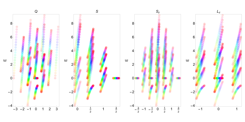
The spectrum for this system, which can be obtained from direct diagonalization of the Hamiltonian, consists of $4^{3}=64$ states in the entire Fock space. When $U=0$, a single state with $Q=-1$, $S=0$, $S_{z}=0$ $L_{z}=0$ has the lowest energy, and a partner with $Q=+1$, $S=0$, $S_{z}=0$, $L_{z}=0$ has the highest energy. Explicitly, the spectrum is not symmetric in $Q$, though of course the spectrum is symmetric in $S_{z}$ and $L_{z}$. When $U$ becomes large, the lowest energy is shared by a degenerate quadruplet of states with $Q=0$, $S=1/2$, $S_{z}=\pm\frac{1}{2}$ and $L_{z}=\pm 1$. At approximately $U^{\triangle}/\kappa=3.61775$ the low-$U/\kappa$ ground state and high-$U/\kappa$ four-plet are degenerate. When $U/\kappa$ is very large the spectrum nearly exhibits symmetry in $Q$.

Spectra, like those shown in Figure 2 and operator overlap factors (18), can be used to directly calculate the single-particle correlator via the spectral decomposition (17). Using the single-particle operators (44) we can also use Monte Carlo to compute the single-particle correlators numerically.

IV.1.1 Ergodicity and the Sign Problem

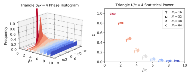
In the language of Refs. Beyl et al. (2018); Wynen et al. (2019) we use the exponential $\alpha=1$ discretization. As detailed in Ref. Wynen et al. (2019) there is a formal ergodicity problem on bipartite lattices. When the lattice is not bipartite the codimension-1 manifolds of exceptional configurations are reduced in dimension and there is no formal ergodicity problem. First, we give a small toy problem confirming this claim and then reproduce the exact results obtained through direct diagonalization. Then, we examine the statistical power for HMC alone as a function of $U/\kappa$ and $\kappa\beta$ and find that, for a given temperature, the sign problem is worst when $U/\kappa=U^{\triangle}/\kappa\approx 3.61775$, the value where the vacuum changes character, as shown in Figure 2.

To visually appreciate that the codimension-1 manifolds that prevent HMC alone from being formally ergodic in the bipartite case are reduced in dimension, consider a problem with $N_{t}=1$ and let $\phi_{x}$ live on spatial site $x$. Then, the product of the fermion determinants is

$$\det M_{p}M_{h}=\frac{4}{9}\left[3\cos\left(\frac{1}{2}\Phi\right)+\sum_{j=1}^{3}\left(2\cosh\left(\kappa+\frac{i}{2}(\Phi-2\phi_{j})\right)+\cosh\left(2\kappa-\frac{i}{2}(\Phi-2\phi_{j})\right)\right)\right]^{2}$$ (47)

where $\Phi=\sum_{x}\phi_{x}$. Figure 3 shows the absolute value (left panel) and complex argument (right panel) of this determinant at $\Phi=0$ and two orthogonal combinations of the field variables. The only zeros are where the lines of different phase meet—in the two-dimensional projection of the phase in Figure 3, points around which the phase winds. As $\Phi$ changes, those points move but they never become extended. So, even with an exponential discretization, the codimension-1 zeros are reduced when the lattice is not bipartite; the fermion determinant allows free exploration the complex plane, rather than constraining it by the reality condition that arises in the bipartite case, as explained in Ref. Wynen et al. (2019).

Figure 3: The absolute value and phase of (47) for $\kappa=1$ and $\Phi=0$, shown as a function of two directions in field space orthogonal to the $\Phi$ direction. In the left panel, yellow indicates large absolute values and purple small ones. In the right panel the color scheme is periodic; the exact zeros occur at the six points on each dark circle where the phase wraps around the point.

Figure 4: The histograms (left) of the phase for two different values of $U/\kappa$ as a function of $\beta$ and the corresponding statistical power (right) with bootstrap errors. In the right panel different $N_{t}$ are shown from left to right: 16, 32, 48, and 64.

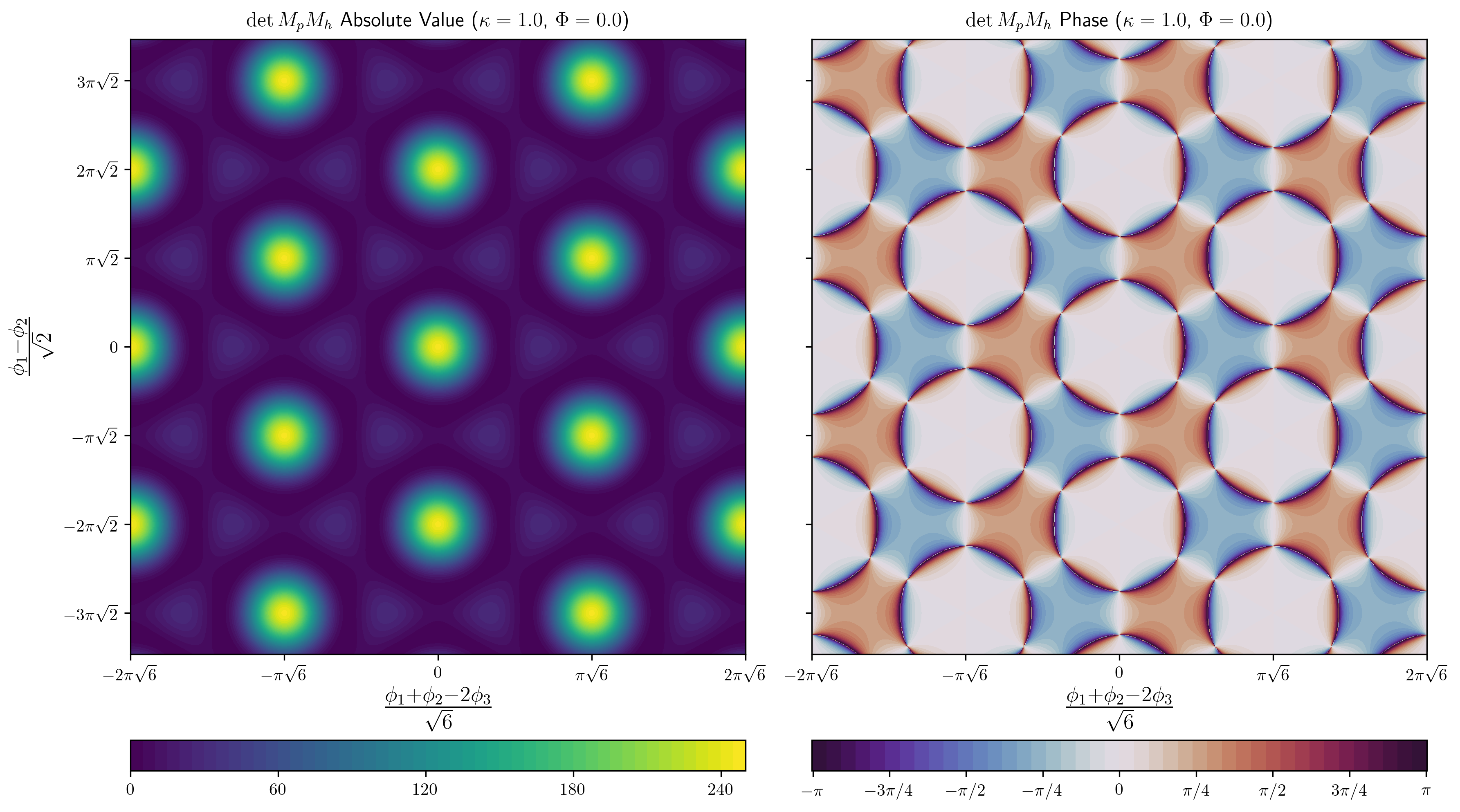
The gaussian part of the weight encourages the fields to stay in the central mode. When the gaussian becomes wider, more than one mode in Figure 3 might become important. There is no formal ergodicity problem, even in the exponential case, and HMC can take us from mode to mode. However, at the mode boundaries, the phase changes rapidly, causing a sign problem. In this small example, if the gaussian is wide enough, HMC can sample trajectories that near this rapid change we would expect to encounter a sign problem, but if the width were very narrow we would not. In examples with more lattice sites and timeslices, the huge growth of phase space of configurations further from $\phi=0$ can counterbalance a narrow gaussian (the width is controlled by $U\beta/N_{t}$), so it is a priori unclear whether increasing $N_{t}$ will help or hurt; since the action is extensive, one expects a sign problem exponentially bad with $\beta$. However, increasing $N_{t}$ also increases the number of variables and the odds that some are near the mode boundaries.

In Figure 4 we show the phase histogram (left panels) and the statistical power (right panels) of ensembles generated with HMC with real valued fields for two values of $U/\kappa$ as functions of $\beta\kappa$. We generated 100,000 trajectories with one molecular dynamics time unit and the number of steps in the leapfrog integrator to give better than 75% acceptance. The histograms are actually results for multiple $N_{t}$s superimposed, to show the very mild sensitivity to the discretization scale. We also generated additional ensembles at $U/\kappa$ from one to nine in integer steps and $U^{\triangle}/\kappa$, and found that the sign problem modestly improved, for fixed $\kappa\beta$, for couplings further from $U^{\triangle}/\kappa$. By analogy, we expect worse sign problems for critical points, where the system must tunnel between qualitatively different ground states.

IV.1.2 Results

Since we can exactly calculate the spectrum and overlap factors for this small problem, we can generate the exact, continuum-limit correlation functions according to the spectral decomposition (17). This provides us a means to directly check the accuracy of our NN method.

We ran HMC in three different ways — on the real plane, on the tangent plane of the main thimble, and on the learnifold. The left panel of Figure 5 shows running averages of the statistical power as a function of Monte Carlo time for $U/\kappa=3$ and $\kappa\beta=8$. After many configurations, $\Sigma$ on real and tangent planes converges to the same small but non-vanishing value, while the neural network produces a markedly greater statistical power. Remember, an improved statistical power indicates an exponential reduction of the sign problem. So, while the sign problem is not solved, per se, we provide evidence here that it is significantly alleviated.

Figure 5: Left panel shows statistical power as a function of sample size on a triangle lattice with $N_{t}=64$, $U/\kappa=3$, $\kappa\beta=8$. Right panel shows statistical power for different parameters on a triangle lattice. Each point was estimated using $10^{5}$ configurations.

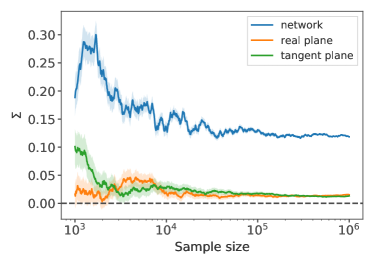
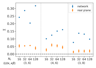
This chosen set of parameters shows the worst statistical power on real and tangent plane out of the sets we tested. See the right panel of Figure 5 for a summary for different parameters. The large variations in $\Sigma$ for neural network based calculations stem from different qualities of the trained models. It should be possible to tune the networks better and thus increase statistical power. These networks perform well enough, however. Generally, we found that the sign problem is not a complete impediment on the triangle and a plain calculation on the real plane with reweighting can suffice.

Figure 6: Single particle correlators $\langle aa^{\dagger}(\tau)\rangle$ on a triangle lattice with $N_{t}=64$, $U/\kappa=3$, $\kappa\beta=8$. Each column shows correlators obtained from ensembles of the given number of configurations, while each row shows a different implementation of HMC. Sample sizes show the total number of Monte Carlo configurations but correlators were measured only on every $10^{\text{th}}$ configuration. The dotted lines are placed at $\max(C)/\sqrt{\text{Sample size}}$ and indicate the scale at which even a sign-problem-free method would show sizeable statistical fluctuations.

Figure 7: Single particle correlators $\langle aa^{\dagger}(\tau)\rangle$ on a triangle lattice for a sample size of $10^{5}$. The low energy correlators are averages of two degenerate results. The top panels show the correlators for different $N_{t}$ from HMC with a neural network and the results from exact diagonalization of the Hamiltonian. The lower panels show the relative error (48). Errors for the low and high energy correlators are labeled $E^{-}$ and $E^{+}$, respectively.

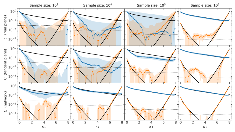
In Figure 6 we show how the different methods’ measurements of diagonalized single-particle correlation functions converge as a function of the number of configurations. With many configurations all three methods reproduce the exact correlators (shown in black). However, the network reproduces the exact results (up to the expected $1/\sqrt{N}$ relative scale from statistical noise) with fewer configurations.

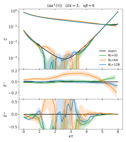
Focusing on learnifold-enhanced HMC calculations, Figure 7 shows single particle correlators for several different parameters and discretization scales measured on ensembles of $10^{5}$ configurations. The figure also shows deviations from the exact results as

$$E=C_{\text{MC}}/C_{\text{exact}}-1\ .$$ (48)

In addition, we compute and diagonalize a variety of correlation functions between bilinear operators, as mentioned in Section II.4 and detailed in Appendix A.1. In Figure 8 we show two — the diagonalized charge-charge and spin-spin correlators. Additional correlators can be found in Figure 15.

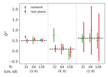
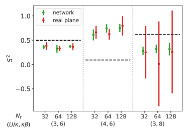
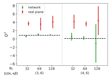
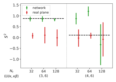
We can use the constant correlators to extract $\left\langle Q^{2}\right\rangle$ and $\left\langle S^{2}\right\rangle$, as explained in Appendix A.2. In Figure 9 we show results for different couplings, temperatures, and discretizations. The learnifold approach yields reduced errors and results consistent with the exact results of $Q^{2}$ for $U/\kappa=3$. The $(U/\kappa,\kappa\beta)=(4,6)$ case seems to have a systematic deviation. It is unsurprising that these parameters yield the worst result as they are closest to $U^{\triangle}/\kappa$. The errors of $S^{2}$ are also reduced by the machine learning approach but a significant systematic deviation from the exact result remains in all cases.

Figure 8: Correlation functions between two charge operators $\rho$ or two $S^{3}$ spin operators separated by euclidean time $\kappa\tau$ on a triangle for different discretization scales given by $N_{t}$ and the exact result (in black). The bottom panels show the relative error (48) for the constant correlator $(0)$ and the average of two heavy correlators $(+)$ which have $k=0$ and $\pm 1$, respectively.

Figure 9: The order parameters $Q^{2}$ (left) and $S^{2}$ (right) calculated with the triangle system with various couplings $U$ and inverse temperatures $\beta$. Shown is a comparison between results calculated with the neural network and on the standard real plane.

IV.2 The Tetrahedron

Many arrangements of four sites are not bipartite. Of these the “most non-bipartite”, and therefore the one where we expect the worst sign problem, is the tetrahedron, where the connectivity matrix is proportional to the adjacency matrix of the complete graph on 4 sites,

$$h=\kappa\left(\begin{array}[]{cccc}0&1&1&1\\ 1&0&1&1\\ 1&1&0&1\\ 1&1&1&0\\ \end{array}\right)$$ (49)

so that each subset of 3 sites forms a frustrated triangle; we label the sites 0-3. The Hamiltonian commutes with the permutation operator $P$ that acts on any triangular face (43) and leaves the other site alone. We conventionally pick the symmetry axis through the fourth site to be the axis of symmetry around which we have a rotational quantum number.

The four irreducible single-particle destruction operators are

$$\hat{O}_{0}^{0} =\frac{1}{2}\sum_{j=0}^{3}a_{j} \hat{O}_{1}^{0} =\frac{1}{2\sqrt{3}}\left(3a_{3}-\sum_{j=0}^{2}a_{j}\right) \hat{O}_{1}^{\pm 1} =\frac{1}{\sqrt{3}}\sum_{j=0}^{2}e^{\pm\frac{2\pi i}{3}j}a_{j}$$ (50)

where the lower index indicates an $L^{2}$-like quantum number $\ell$ and the upper index an $L_{z}$-like quantum number $m$. The free Hamiltonian may be written in terms of these operators,

$$H_{0}=\kappa\left[\left(-3\hat{O}_{0}^{0\dagger}\hat{O}_{0}^{0}+\sum_{m=-1}^{1}\hat{O}_{1}^{m\dagger}\hat{O}_{1}^{m}\right)-(a\rightarrow b)\right]$$ (51)

and the translationally-invariant interaction term transforms as an $\ell=0$, $m=0$ “spherical tensor”. Therefore, these are good quantum numbers and correlation functions put into this basis are diagonal.

IV.2.1 Results

We expect the sign problem to be worse than on a triangle because the tetrahedron is substantially more frustrated since it has four triangular faces. This is an opportunity to test our method in a system where calculations on the real plane are, as far as we can tell, just not possible.

Figure 10: Left panel shows the statistical power as a function of sample size on a tetrahedron lattice with $N_{t}=64$, $U/\kappa=3$, $\kappa\beta=6$. Right panel shows statistical power for different parameters on a triangle lattice. Each point was estimated using $10^{6}$ configurations.

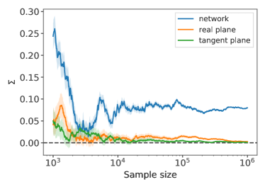
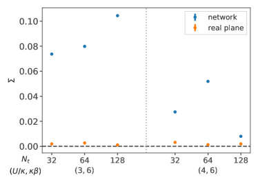
Indeed, HMC on both the real and tangent planes has essentially 0 statistical power as shown in the left panel of Figure 10, an extremely difficult sign problem. In contrast, the neural network method converges to a finite statistical power. Even though this value is small, it is sufficient as shown below. The right panel of Figure 10 shows this improvement in statistical power holds for all the ensembles we consider.

Figure 11: Single particle correlators $\langle aa^{\dagger}(\tau)\rangle$ on a tetrahedron lattice with $N_{t}=64$, $U/\kappa=3$, $\kappa\beta=6$. Each column shows correlators obtained from ensembles of the given number of configurations, while each row shows a different implementation of HMC. Correlators are computed only on every $10^{\text{th}}$ configuration. The dotted lines are placed at $\max(C)/\sqrt{\text{Sample size}}$ and indicate the scale at which even a sign-problem-free method would show sizeable statistical fluctuations.

Figure 12: Single particle correlators $\langle aa^{\dagger}\rangle$ on a tetrahedron lattice. The low energy correlators are averages of three degenerate results. The top panels show the correlators for different $N_{t}$ from HMC with neural network and the results from exact diagonalization of the Hamiltonian. The lower panels show the relative error (48). Errors for the low and high energy correlators are labeled $E^{-}$ and $E^{+}$, respectively.

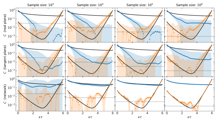
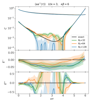
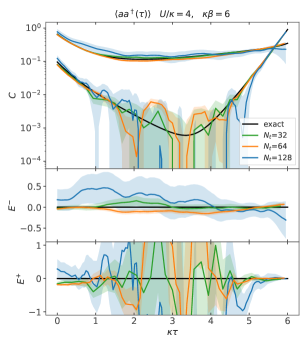
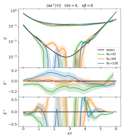
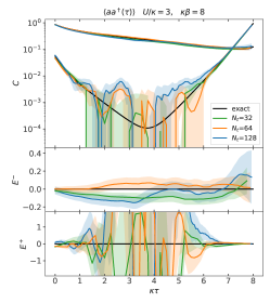
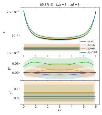
Figure 11 shows the drastic improvement obtained when simulating with the neural network. By studying the single-particle correlators, it is apparent that while the network method converges to the exact answer, the real and tangent plane methods are completely ineffective — their uncertainties remain large and their match to the exact results poor.

In Figure 12 we show network-method results for different discretizations, and their relative errors $E$ (48). Those correlators were computed on an ensemble of $10^{6}$ configurations, measuring on only every $10^{\text{th}}$ configuration to reduce autocorrelations. The light correlator is an average of the $\ell=1$ triplet of correlation functions. The error of the heavy correlator grows for intermediate euclidean time, but this is expected given the concrete sample size, see Figure 11.

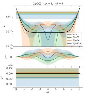
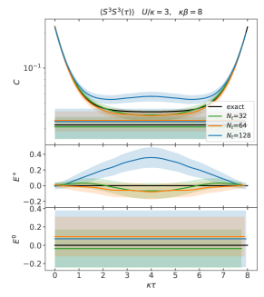
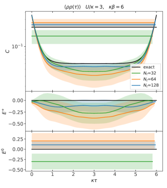
In addition, we computed bilinear correlation functions as described in Section II.4 and Section A.1. Figure 13 shows the continuum-limit convergence of the charge-charge and $S^{3}$-$S^{3}$ correlators projected to the singlet and triplet (as in (50)) towards the exact result. Additional examples can be found in Figure 16.

In Figure 14 we show $\left\langle Q^{2}\right\rangle$ and $\left\langle S^{2}\right\rangle$, see Appendix A.2 for their derivation. Calculations on the real plane show significant systematic deviations from the exact result. Calculations on learnifolds, however, have improved $Q^{2}$ for all $U/\kappa$ and $S^{2}$ for $U/\kappa=3$ to the point where they agree with the exact result. Curiously, $S^{2}$ for $(U/\kappa,\kappa\beta)=(4,6)$ is worse on the learnifold. Note, however, that while the real plane results are consistent with the exact value of $S^{2}$, they are also consistent with zero.

Figure 13: Correlation functions between two charge operators $\rho$ or two $S^{3}$ spin operators on a tetrahedron. The bottom panels show the relative error (48) for the constant correlator $E^{0}$ and the average of three heavy correlators $E^{+}$, respectively.

Figure 14: The order parameters $Q^{2}$ (left) and $S^{2}$ (right) calculated with the tetrahedron system with different couplings $U$ and inverse temperature $\beta$. Shown is a comparison between results calculated with the neural network and on the standard real plane.

V Conclusions

In this work we adapted the learnifold method proposed by Alexandru, Bedaque, Lamm, and Lawrence Alexandru et al. (2017b) to alleviate the sign problem in small, frustrated Hubbard model examples. As shown in Figs. 5 and 10, our method definitively improves the statistical power, thus providing an exponential improvement in the sign problem. With the NN, it reproduces results obtained from exact diagonalization on a variety of correlation functions, c.f. Figures 7, 8, 15, 12, 13, 16. The agreement with exact results provides a posteriori evidence that we have an accurate, ergodic method.

By approximating the holomorphic flow with a neural network, we have developed an HMC method well-suited for tackling sign problems in the Hubbard model. As opposed to most previous work involving Lefschetz thimbles, our method does not rely on obtaining the precise location of the main thimble nor on the locations of less critical thimbles. In fact, our neural networks perform better when not using prior knowledge of thimble locations. The reason is two-fold. First, during HMC evolution, the gaussian part of our action drives configurations to regions that are not dominated by a single thimble, bur rather multiple thimbles. If we instead only trained on the main thimble, HMC would quickly force configurations into regions outside the trained network and we immediately encounter a numerical runaway problem — the imaginary part of the fields become arbitrarily large in an attempt to minimize the action. Second, our goal is to alleviate the sign problem to a point where standard reweighting techniques can be applied to obtain sufficiently accurate observables. Thus our maximum flow time was relatively small, yet sufficient to obtain accurate results. The modest flow times also prevented us from coming too close to points where the integration kernel vanishes, which in turn kept any ergodicity issues at bay. Though integrating directly on the thimbles eliminates the sign problem altogether, we believe that determining the exact location of these manifolds and the subsequent manifold integration is a daunting task (perhaps as difficult as the original sign problem), and becomes only more difficult if one considers gauge theories in higher dimensions.

A drawback of our method is still the need to calculate the determinant of a Jacobian induced by the complexified fields. Though our network was able to calculate the Jacobian much more quickly than a direct numerical flowing of the Jacobian as needed by holomorphic flow, the calculation still scales with the cubic power of the spacetime volume. Thus we anticipate that calculations of larger dimensional systems with our network method will ultimately run into this scaling barrier. We are actively researching methods to reduce this computational scaling, and we see some promise in networks that work directly with complex variables, see Appendix B.

The sign problem we addressed was due to the non-bipartite spatial lattices, thus providing a basis for extensions to quasi-zero-dimensional systems like $C_{20}$ and the buckyball $C_{60}$. Our framework is nonetheless easily adapted to other sign problems. In future work, we anticipate simulating systems away from half filling and extended models with sufficiently strong non-local couplings Buividovich et al. (2016), both of which suffer a sign problem not only extensive in euclidean time but also in space.

Appendix A Correlation Functions of Bilinear Operators

Spin-spin correlation functions are correlation functions between local spin operators $S_{x}^{i}$ where $x$ is a lattice site and $i$ runs over the indices of the Pauli matrices,

$$S_{x}^{i}=\frac{1}{2}\sum_{ss^{\prime}}c_{xs}\sigma^{i}_{ss^{\prime}}{c}^{\dagger}_{xs^{\prime}}$$ (52)

and where $c$ is a doublet of operators,

$$c_{xs}=\left(\begin{array}[]{c}a_{x}\\ (-\sigma_{\kappa})^{x}{b}^{\dagger}_{x}\end{array}\right)$$ (53)

where $\sigma_{\kappa}$ is $+1$ on bipartite lattices and must be $-1$ on non-bipartite lattices, following the convention of Isle (bipartite graphs can also have $\sigma_{\kappa}=-1$). In Ref. Buividovich et al. (2018) the authors also define, just after (1), the electric charge operator

$$\rho_{x}={c}^{\dagger}_{x,\uparrow}c_{x,\uparrow}+{c}^{\dagger}_{x,\downarrow}c_{x,\downarrow}-1$$ (54)

which can be rewritten as $\rho_{x}=1-2S^{0}_{x}$, where the $0^{th}$ Pauli matrix is the $2\times 2$ identity matrix. The $S$ operators are Hermitian. Rewriting those operators into the Isle basis,

$$S^{0}_{x} =\frac{1}{2}\left[a_{x}{a}^{\dagger}_{x}-b_{x}{b}^{\dagger}_{x}+1\right] S^{1}_{x} =\frac{1}{2}(-\sigma_{\kappa})^{x}\left[{b}^{\dagger}_{x}{a}^{\dagger}_{x}+a_{x}b_{x}\right]$$

$$\rho_{x} =n^{a}_{x}-n^{b}_{x}=1-2S^{0}_{x}=b_{x}{b}^{\dagger}_{x}-a_{x}{a}^{\dagger}_{x} S^{2}_{x} =\frac{i}{2}(-\sigma_{\kappa})^{x}\left[{b}^{\dagger}_{x}{a}^{\dagger}_{x}-a_{x}b_{x}\right]$$ (55)

$$n_{x} =n^{a}_{x}+n^{b}_{x}=1-2S^{3}_{x}=a^{\dagger}_{x}a_{x}+b^{\dagger}_{x}b_{x} S^{3}_{x} =\frac{1}{2}\left[a_{x}{a}^{\dagger}_{x}+b_{x}{b}^{\dagger}_{x}-1\right]$$

where the $\sigma_{\kappa}$ squares away when two $b$ operators are multiplied and no sum is implied on the right-hand sides. The other two spin bilinears have absolute charge 2,

$${(S{{}^{+}_{+}})}_{x} ={a}^{\dagger}_{x}b_{x} {(S{{}^{-}_{-}})}_{x} ={b}^{\dagger}_{x}a_{x}.$$ (56)

There are, of course, other doubly-charged operators but none that live on a single site, by Pauli exclusion.

The three spin operators obey the commutation relation

$$\left[S_{x}^{i},S_{y}^{j}\right]=i\delta_{xy}\epsilon^{ijk}S_{x}^{k}$$ (57)

which may be checked explicitly by writing out the operators and using the anticommutation properties of $a$ and $b$. By a similar exercise one may show

$$\left[S_{x}^{0},S_{y}^{j}\right]=0.$$ (58)

Single-particle and single-hole operators $\mathcal{O}$ with a definite third component of spin $s_{3}$ obey the operator eigenvalue equation

$$[S_{x}^{3},\mathcal{O}_{y}]=s_{3}\mathcal{O}_{y}\delta_{xy}.$$ (59)

This equation is satisfied when $(\mathcal{O},s_{3})=(a,+\frac{1}{2})$, $({a}^{\dagger},-\frac{1}{2})$, $(b,+\frac{1}{2})$, and $({b}^{\dagger},-\frac{1}{2})$. Single-particle and single-hole operators $\mathcal{O}$ with a definite electric charge $q$ obeys the operator eigenvalue equation

$$[\rho_{x},\mathcal{O}_{y}]=q\mathcal{O}_{y}\delta_{xy}.$$ (60)

This equation is satisfied when $(\mathcal{O},q)=(a,-1)$, $({a}^{\dagger},+1)$, $(b,+1)$, and $({b}^{\dagger},-1)$. Note that the signs differ from the $S^{3}$ case.

One may also construct spin raising and lowering operators in the standard way,

$$S^{+}_{x}=S^{1}_{x}+iS^{2}_{x} =(-\sigma_{\kappa})^{x}a_{x}b_{x} S^{-}_{x}=S^{1}_{x}-iS^{2}_{x} =(-\sigma_{\kappa})^{x}{b}^{\dagger}_{x}{a}^{\dagger}_{x}$$ (61)

which obey the eigenvalue relations

$$[S_{x}^{3},S^{\pm}_{y}]=\pm S^{\pm}_{y}\delta_{xy},$$ (62)

which can be shown using the single-particle and single-hole eigenvalue equations and the Leibniz rule.

The construction of the number operators proceeds in a similar fashion,

$$\delta_{xx}-n^{p}_{x} =S^{0}_{x}+S^{3}_{x}=a_{x}{a}^{\dagger}_{x}=\delta_{xx}-{a}^{\dagger}_{x}a_{x}$$ (63)

$$n^{h}_{x} =S^{0}_{x}-S^{3}_{x}=-b_{x}{b}^{\dagger}_{x}+\delta_{xx}=-\delta_{xx}+{b}^{\dagger}_{x}b_{x}+\delta_{xx}={b}^{\dagger}_{x}b_{x}.$$ (64)

We can of course drop the constant term in the first definition. The number operators obey the equations

$$\left[n^{p}_{x},a_{y}\right] =-a_{y}\delta_{xy} \left[n^{p}_{x},{a}^{\dagger}\right] =+{a}^{\dagger}_{y}\delta{xy}$$ (65)

and similarly for holes. It is easy to see using the eigenoperator equations (59) and (60) and the Leibniz rule that these operators commute with the local electric charge and spin, so that they have vacuum quantum numbers, while the doubly-charged operators satisfy

$$[\rho_{x},{(S{{}^{+}_{+}})}_{y}] =+2{(S{{}^{+}_{+}})}_{y}\delta_{x}y [\rho_{x},{(S{{}^{-}_{-}})}_{y}] =-2{(S{{}^{-}_{-}})}_{y}\delta_{x}y$$ (66)

and are spin-0 because they commute with the spin operators. The one-point functions may be computed by Wick contraction

$$\frac{1}{N_{t}}\sum_{t}\langle n^{p}_{x}\rangle =\left\langle 1-\frac{1}{N_{t}}\sum_{t}P_{xtxt}\right\rangle \frac{1}{N_{t}}\sum_{t}\langle n^{h}_{x}\rangle =\left\langle 1-\frac{1}{N_{t}}\sum_{t}H_{xtxt}\right\rangle$$ (67)

where we denoted the Wick contraction of $a_{x,t_{f}}{a}^{\dagger}_{y,t_{i}}=(M^{p})^{-1}_{xt_{f}yt_{i}}\equiv P_{xt_{f}yt_{i}}$, defining the particle propagator $P$, and similarly for holes $b_{x,t_{f}}{b}^{\dagger}_{y,t_{i}}=(M^{h})^{-1}_{xt_{f}yt_{i}}\equiv H_{xt_{f}yt_{i}}$ the hole propagator. These may be combined according to (A) to get one-point expectation values for $n_{x}$, $\rho_{x}$, and $S^{3}_{x}$. Bilinears not having vacuum quantum numbers have vanishing one-point expectation values.

A.1 Correlation Functions

Now we can write two-point correlation functions

$$C^{uv}_{xy}(\tau)=\frac{1}{N_{t}}\sum_{t}\left\langle S^{u}_{x,t+\tau}S^{v}_{y,t}\right\rangle$$ (68)

and we do not need to track time separately, until we start analyzing how to actually analyze these correlation functions via their spectral decompositions, though we always put the $x$ position at the initial time $i=t$ and the $y$ position at the final time $f=t+\tau$, so one can read $x$ and $y$ as superindices. When calculating numerically we sum over all initial timeslices $t$ to ensure the only time dependence is on the time difference $\tau$. In these correlator expressions $x$ and $y$ are unsummed.

The simplest correlation function is between $S^{+}$ and $S^{-}$,

$$C^{+-}_{xy}=\left\langle S^{+}_{x}S^{-}_{y}\right\rangle=(-\sigma_{\kappa})^{x+y}\left\langle a_{x}b_{x}{b}^{\dagger}_{y}{a}^{\dagger}_{y}\right\rangle =(-\sigma_{\kappa})^{x+y}\left\langle P_{xy}H_{xy}\right\rangle$$ (69)

$$C^{-+}_{xy}=\left\langle S^{-}_{x}S^{+}_{y}\right\rangle=(-\sigma_{\kappa})^{x+y}\left\langle{b}^{\dagger}_{x}{a}^{\dagger}_{x}a_{y}b_{y}\right\rangle =(-\sigma_{\kappa})^{x+y}\left\langle(\delta_{yx}-b_{y}{b}^{\dagger}_{x})(\delta_{yx}-a_{y}{a}^{\dagger}_{x})\right\rangle$$

$$=(-\sigma_{\kappa})^{x+y}\left\langle(\delta_{yx}-H_{yx})(\delta_{yx}-P_{yx})\right\rangle$$ (70)

where we have taken advantage of the anticommutator rules and that the Wick contractions yield the particle and hole propagators $P$ and $H$ (suppressing the time dependence for clarity). At half filling on a bipartite lattice, the cost to create or destroy a spin from the vacuum should be equal and the correlators should match, in the limit of large statistics. At equal time $\tau=0$, these correlation functions provide access to the spin-flip information Colmenarez et al. (2019).

Correlations between the number operator $n^{p}$ and itself or $n^{h}$ are also simple to write,

$$C^{ph}_{xy}=\left\langle n^{p}_{x}n^{h}_{y}\right\rangle=\left\langle(\delta_{xx}-a_{x}{a}^{\dagger}_{x})(\delta_{yy}-b_{y}{b}^{\dagger}_{y})\right\rangle =\left\langle(\delta_{xx}-P_{xx})(\delta_{yy}-H_{yy})\right\rangle$$ (71)

$$C^{pp}_{xy}=\left\langle n^{p}_{x}n^{p}_{y}\right\rangle=\left\langle(\delta_{xx}-a_{x}{a}^{\dagger}_{x})(\delta_{yy}-a_{y}{a}^{\dagger}_{y})\right\rangle =\left\langle\delta_{xx}\delta_{yy}-a_{x}{a}^{\dagger}_{x}\delta_{yy}-\delta{xx}a_{y}{a}^{\dagger}_{y}+a_{x}{a}^{\dagger}_{x}a_{y}{a}^{\dagger}_{y}\right\rangle$$

$$=\left\langle\delta_{xx}\delta_{yy}-a_{x}{a}^{\dagger}_{x}\delta_{yy}-\delta_{xx}a_{y}{a}^{\dagger}_{y}+a_{x}(\delta_{xy}-a_{y}{a}^{\dagger}_{x}){a}^{\dagger}_{y}\right\rangle$$

$$=\left\langle\delta_{xx}\delta_{yy}-P_{xx}\delta_{yy}-\delta_{xx}P_{yy}+P_{xy}\delta_{xy}+P_{xx}P_{yy}-P_{xy}P_{yx}\right\rangle$$ (72)

and we can interchange the p/h species superscripts by exchanging the $P$ and $H$ propagators.While these correlators are between operators as simple as $S^{+}$ and $S^{-}$, computationally these Wick contractions are tougher to compute because they are “quark-line disconnected”.

We can also build correlators between the spin operators $S^{i}$. For example $C^{11}$ is given by

$$C^{11}_{xy}=\left\langle S^{1}_{x}S^{1}_{y}\right\rangle =\frac{1}{4}(-\sigma_{\kappa})^{x+y}\left\langle\left[{b}^{\dagger}_{x}{a}^{\dagger}_{x}+a_{x}b_{x}\right]\left[{b}^{\dagger}_{y}{a}^{\dagger}_{y}+a_{y}b_{y}\right]\right\rangle$$

$$=\frac{1}{4}(-\sigma_{\kappa})^{x+y}\left\langle a_{x}{a}^{\dagger}_{y}b_{x}{b}^{\dagger}_{y}+(\delta_{yx}-a_{y}{a}^{\dagger}_{x})(\delta_{yx}-b_{y}{b}^{\dagger}_{x})\right\rangle$$

$$=\frac{1}{4}(-\sigma_{\kappa})^{x+y}\left\langle P_{xy}H_{xy}+(\delta_{yx}-P_{yx})(\delta_{yx}-H_{yx})\right\rangle$$ (73)

where we have used the fact that we will only get a non-zero result if we have the same number of $a$s as ${a}^{\dagger}$s (and likewise for $b$) to drop the four-dagger and no-dagger terms. Computing $C^{22}_{xy}$ requires

$$\left\langle S^{2}_{x}S^{2}_{y}\right\rangle =\frac{1}{4}(-\sigma_{\kappa})^{x+y}\left\langle\left[{b}^{\dagger}_{x}{a}^{\dagger}_{x}-a_{x}b_{x}\right]\left[a_{y}b_{y}-{b}^{\dagger}_{y}{a}^{\dagger}_{y}\right]\right\rangle$$ (74)

though when written out in their complete glory, only the non-vanishing operator content in $\left\langle S^{1}_{x}S^{1}_{y}\right\rangle$ remains, so $C^{22}_{xy}=C^{11}_{xy}$ configuration-by-configuration (the vanishing operators have the opposite sign). In fact, using the definition of the spin raising and lowering operators (61) one concludes

$$C^{11}_{xy}+C^{22}_{xy} =\frac{1}{2}\left(C^{+-}_{xy}+C^{-+}_{xy}\right) C^{12}_{xy}-C^{21}_{xy} =\frac{i}{2}\left(C^{+-}_{xy}-C^{-+}_{xy}\right)$$ (75)

and we have explicitly checked the first identity by computing the Wick contractions (69), (70), and (73), and the fact that $C^{22}_{xy}=C^{11}_{xy}$. It is easy to show that once the all-dagger or no-dagger operators are dropped,

$$\left\langle S^{1}_{x}S^{2}_{y}\right\rangle =-\left\langle S^{2}_{x}S^{1}_{y}\right\rangle C^{12}_{xy} =\frac{i}{4}\left(C^{+-}_{xy}-C^{-+}_{xy}\right)$$ so that (76)

which may be checked explicitly, and is true configuration-by-configuration.

The other two spins $S^{0}$ and $S^{3}$ do not enjoy such simplifications, because unlike the raising and lowering operators the number operators (64) have vacuum quantum numbers, so there are no zero- or four-dagger terms which may be dropped from the Wick contractions. We are stuck computing four correlators,

$$C^{00}_{xy} =\frac{1}{4}\left(C^{pp}_{xy}+C^{hh}_{xy}-C^{ph}_{xy}-C^{hp}_{xy}+\left\langle 1-n^{p}_{x}-n^{p}_{y}+n^{h}_{x}+n^{h}_{y}\right\rangle\right)$$

$$C^{03}_{xy} =\frac{1}{4}\left(C^{pp}_{xy}-C^{hh}_{xy}+C^{ph}_{xy}-C^{hp}_{xy}+\left\langle 1-n^{p}_{x}-n^{p}_{y}+n^{h}_{x}-n^{h}_{y}\right\rangle\right)$$

$$C^{30}_{xy} =\frac{1}{4}\left(C^{pp}_{xy}-C^{hh}_{xy}-C^{ph}_{xy}+C^{hp}_{xy}+\left\langle 1-n^{p}_{x}-n^{p}_{y}-n^{h}_{x}+n^{h}_{y}\right\rangle\right)$$

$$C^{33}_{xy} =\frac{1}{4}\left(C^{pp}_{xy}+C^{hh}_{xy}+C^{ph}_{xy}+C^{hp}_{xy}+\left\langle 1-n^{p}_{x}-n^{p}_{y}-n^{h}_{x}-n^{h}_{y}\right\rangle\right)$$

$$\text{and we define }C^{\rho\rho}_{xy} =C^{pp}_{xy}+C^{hh}_{xy}-C^{ph}_{xy}-C^{hp}_{xy}$$ (77)

$$C^{\rho n}_{xy} =C^{pp}_{xy}-C^{hh}_{xy}+C^{ph}_{xy}-C^{hp}_{xy}$$ (78)

$$C^{n\rho}_{xy} =C^{pp}_{xy}-C^{hh}_{xy}-C^{ph}_{xy}+C^{hp}_{xy}$$ (79)

$$C^{nn}_{xy} =C^{pp}_{xy}+C^{hh}_{xy}+C^{ph}_{xy}+C^{hp}_{xy}$$ (80)

so that a $\rho$ superscript indicates the charge operator (A) and an $n$ superscript the total number operator. The Wick contractions may be explicitly computed or built by rewriting the definition of the number operators (64) as

$$S^{0}_{x} =\frac{1}{2}\left(1+n^{h}_{x}-n^{p}_{x}\right) S^{3}_{x} =\frac{1}{2}\left(1-n^{h}_{x}-n^{p}_{x}\right)$$ (81)

and using the particle-hole (71) and particle-particle (72) correlators and the one-point functions (67). Note that $S^{1,2}$ cannot be correlated with $S^{0,3}$ because each term would not have the right constituent operator content to contract completely, so those correlators automatically vanish.

The doubly charged operators have simple Wick contractions. Note that ${(S{{}^{+}_{+}})}^{\dagger}={(S{{}^{-}_{-}})}$ so that

$${(C{{}^{+}_{+}}{{}^{-}_{-}})}_{xy} =\left\langle{a}^{\dagger}_{x}b_{x}{b}^{\dagger}_{y}a_{y}\right\rangle=\left\langle{a}^{\dagger}_{x}a_{y}b_{x}{b}^{\dagger}_{y}\right\rangle=\left\langle(\delta_{yx}-a_{y}{a}^{\dagger}_{x})b_{x}{b}^{\dagger}_{y}\right\rangle=\left\langle(\delta_{yx}-P_{yx})H_{xy}\right\rangle$$ (82)

$$C{{}^{-}_{-}}{{}^{+}_{+}} =\left[C{{{}^{+}_{+}}{{}^{-}_{-}}}\text{ with }P\leftrightarrow H\right].$$ (83)

Based on the exact results, a Lepage-style argument Lepage (1990) suggests these doubly-charged correlators should suffer from a signal-to-noise problem.

A.2 Conserved Quantities

When the Hamiltonian takes a Hubbard-Coulomb-like form,

$$H=-\sum_{xy}\left({a}^{\dagger}_{x}h_{xy}a_{y}+\sigma_{\kappa}{b}^{\dagger}_{x}h_{xy}b_{y}\right)+\frac{1}{2}\sum_{xy}\rho_{x}V_{xy}\rho_{y}$$ (84)

some of the bilinears may correspond to conserved quantities. For example, we can calculate the commutator with a local charge density operator,

$$[H,\rho_{z}] =\left[\sum_{xy}{a}^{\dagger}_{x}h_{xy}a_{y}+\ \sigma_{\kappa}{b}^{\dagger}_{x}h_{xy}b_{y},\rho_{z}\right]$$ (85)

$$=\sum_{x}-{a}^{\dagger}_{x}h_{xz}a_{z}+\sum_{y}{a}^{\dagger}_{z}h_{zy}a_{y}-\sigma_{\kappa}(a\leftrightarrow b)$$ (86)

where we immediately dropped the interaction term since the charge operator commutes with itself. If we sum $z$ over all space the two terms cancel, so that the total charge

$$Q=\sum_{z}\rho_{z}$$ (87)

is conserved. One similarly finds the total spins in each direction conserved,

$$\left[H,S^{i}\right] =0 S^{i}=\sum_{z}S^{i}_{z}$$ (88)

for $i\in\{1,2,3\}$ and in fact the total spin also commutes with the Hamiltonian

$$[H,S^{2}] =0 S^{2} =\sum_{i}(S^{i})^{2}.$$ (89)

When the operators are conserved, their two-point correlation functions are constant,

$$C^{QQ}(\tau) =\frac{1}{\mathcal{Z}}\text{tr}\left[Q(\tau)Q(0)e^{-\beta H}\right] =\frac{1}{\mathcal{Z}}\text{tr}\left[e^{+H\tau}Q(0)e^{-H\tau}Q(0)e^{-\beta H}\right]$$

$$=\frac{1}{\mathcal{Z}}\text{tr}\left[Q(0)e^{-H\tau}Q(0)e^{-(\beta-\tau)H}\right] =\frac{1}{\mathcal{Z}}\text{tr}\left[Q(0)Q(0)e^{-\beta H}\right]$$ (90)

where we wrote the Heisenberg-picture $Q(\tau)$ in terms of the zero-time operator and the Hamiltonian and repeatedly used the fact that $Q$ commutes with the Hamiltonian. We can turn this relation on its head and get an estimate for the equal-time correlator $\left\langle Q^{2}\right\rangle$ by averaging over the temporal separation,

$$\left\langle Q^{2}\right\rangle=\frac{1}{N_{t}}\sum_{\tau}C^{QQ}(\tau)=\frac{1}{N_{t}}\sum_{\tau}C^{\rho\rho}_{++}(\tau),$$ (91)

where a $+$ subscript indicates that the spatial index is summed over—in this case, implementing (87). This same observation holds for the total spin operators $S^{i}$ (and therefore also for $S^{\pm}$), with the Hamiltonian shown above. We can measure the mean-squared magnetization $\left\langle S^{2}\right\rangle$ by

$$\left\langle S^{2}\right\rangle=\sum_{i=1}^{3}\frac{1}{N_{t}}\sum_{\tau}C^{ii}_{++}(\tau)$$ (92)

On small test examples one observes numerically that the correlators are flat with the exponential discretization and seem linear with time in the diagonal discretization; averaging properly still yields good values—for an explicit example see the last appendix of Ref. Wynen et al. (2019).

A.3 Numerical Results

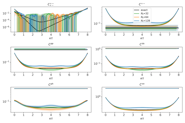
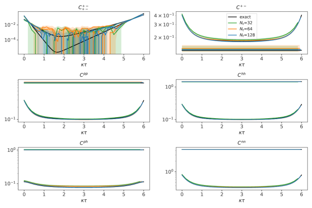
This section shows results for additional correlators that are not covered in the main text. Correlators in Figures 15 and 16 are computed on the same ensembles (“network”) as those in Sections IV.1.2 and IV.2.1, respectively.

Figure 15: Numerical results for some correlation functions on a triangle lattice with $U/\kappa=3$, $\kappa\beta=8$ and $10^{5}$ configurations.

Figure 16: Numerical results for some correlation functions on a tetrahedron lattice with $U/\kappa=3$, $\kappa\beta=8$ and $10^{5}$ configurations.

Appendix B Coupling Layers

As described above, the networks used here have a significant disadvantage, their Jacobians are expensive to compute. Using coupling layers with a suitable coupling rule as introduced in Ref. Dinh et al. (2014) instead of dense layers, can effectively reduce that cost to zero in most applications.

For $x,y\in\mathds{R}^{\Lambda}$, let $\{A,B\}$ be a partition of the integer interval $\llbracket 1,\Lambda\rrbracket$. $\Lambda$ is the lattice spacetime volume $N_{x}N_{t}$ and we restrict ourselves to even $\Lambda$ and $|A|=|B|=\Lambda/2$. A coupling layer is defined as

$$f(x)=\begin{cases}y_{A}=x_{A}\\ y_{B}=g(x_{A},x_{B})\end{cases}$$ (93)

Here, we focus on affine coupling layers which have a coupling rule of 

$$g(x_{A},x_{B})=x_{B}\odot s(x_{A})+t(x_{A})\ ,$$ (94)

where $\odot$ denotes element wise multiplication and $s$ and $t$ are arbitrary functions which can be parameterized through neural networks. The Jacobian determinant of a network made out of layers, meaning $\text{NN}(x)=f^{n}(f^{n-1}(\cdots f^{1}(x)))$, factorizes into separate determinants for each layer:

$$\det J=\det\frac{\partial\text{NN}}{\partial x}=\det\bigg{(}\frac{\partial f^{n}(x)}{\partial x}\bigg{)}\det\bigg{(}\frac{\partial f^{n-1}(x)}{\partial x}\bigg{)}\cdots\det\bigg{(}\frac{\partial f^{1}(x)}{\partial x}\bigg{)}$$ (95)

In the case of affine coupling layers, the rows and columns of the layer Jacobians can be permuted under the determinants such that for each layer $A=\llbracket 1,\Lambda/2\rrbracket$, $B=\llbracket\Lambda/2+1,\Lambda\rrbracket$ thus making the matrices triangular and the determinant fast to compute:

$$\det\bigg{(}\frac{\partial f}{\partial x}\bigg{)}=\det\begin{pmatrix}\mathds{1}_{\Lambda/2}&0\\ \frac{\partial y_{B}}{\partial x_{A}}&s(x_{A})\end{pmatrix}=\prod_{i=1}^{\Lambda/2}\,{s(x_{A})}_{i}\ ,$$ (96)

where $s(x_{A})$ is to be understood as a diagonal matrix in the second expression.

This procedure can not be applied with the approach taken in this work as the transformation Eq. (26) has Jacobian (see Eq. (28))

$$\det J[\phi]=\det\bigg{(}\mathds{1}+i\frac{\partial\text{NN}(\phi)}{\partial\phi}\bigg{)}\ .$$ (97)

This determinant does not factorize and we can not bring the derivative of each layer into triangular shape. $A$ and $B$ can also not be chosen such that the product of layers $\partial\text{NN}(\phi)/\partial\phi$ itself is triangular because that would mean that not all components of $\phi$ could influence all components of $\tilde{\phi}$ which would limit the expressive power of the network.

The root cause for the problem is the different treatment of real and imaginary parts in Eq. (26) because it leads to the “$\mathds{1}+$” in the determinant. A potential solution would be changing the transformation to $\tilde{\phi}=\text{NN}(\phi)$. However, this requires networks which deal with complex numbers and forgoes the potential benefits of Eq. (26) described in the main text. It is not trivial to formulate complex valued neural networks. One difficulty comes from the loss functions which are typically non-analytic. This problem can be avoided by using Wirtinger calculus to construct an optimization procedure Brandwood (1983); Kreutz-Delgado (2009). Another difficulty is finding complex activation functions Scardapane et al. (2018). Here, the problem is complicated further because the chain rule of Wirtinger derivatives contains a sum:

$$z=f(y),\,y=g(x)\quad\Rightarrow\quad\frac{\partial z}{\partial x}=\frac{\partial f}{\partial y}\frac{\partial g}{\partial x}+\frac{\partial f}{\partial y^{\ast}}\frac{\partial g^{\ast}}{\partial x}$$ (98)

This would ultimately produce a sum in the determinant of the Jacobian, preventing factorization. The efficient Jacobian of Eq. (96) can thus only be realized with holomorphic neural networks, which implies holomorphic activation functions. For this first stage of our work we relied on professionally-optimized, third-party machine learning libraries but support for complex-valued networks is currently incomplete. We plan to develop an implementation with support for complex-valued coupling layers and pursue the approach described here.

References

- Splittorff and Verbaarschot (2007) K. Splittorff and J. J. M. Verbaarschot, “The QCD Sign Problem for Small Chemical Potential,” Phys. Rev. D75, 116003 (2007), arXiv:hep-lat/0702011 [HEP-LAT] .
- Danzer et al. (2009) Julia Danzer, Christof Gattringer, Ludovit Liptak, and Marina Marinkovic, “A Study of the sign problem for lattice QCD with chemical potential,” Phys. Lett. B682, 240–245 (2009), arXiv:0907.3084 [hep-lat] .
- Garron and Langfeld (2016) Nicolas Garron and Kurt Langfeld, “Anatomy of the sign-problem in heavy-dense QCD,” Eur. Phys. J. C76, 569 (2016), arXiv:1605.02709 [hep-lat] .
- Hsu and Reeb (2010) Stephen D. H. Hsu and David Reeb, “On the sign problem in dense QCD,” Int. J. Mod. Phys. A25, 53–67 (2010).
- Goy et al. (2017) V. A. Goy, V. Bornyakov, D. Boyda, A. Molochkov, A. Nakamura, A. Nikolaev, and V. Zakharov, “Sign problem in finite density lattice QCD,” PTEP 2017, 031D01 (2017), arXiv:1611.08093 [hep-lat] .
- Shindler et al. (2015) Andrea Shindler, Thomas Luu, and Jordy de Vries, “Nucleon electric dipole moment with the gradient flow: The -term contribution,” Phys. Rev. D92, 094518 (2015), arXiv:1507.02343 [hep-lat] .
- Gavai and Gupta (2008) R. V. Gavai and Sourendu Gupta, “QCD at finite chemical potential with six time slices,” Phys. Rev. D78, 114503 (2008), arXiv:0806.2233 [hep-lat] .
- Dragos et al. (2019) Jack Dragos, Thomas Luu, Andrea Shindler, Jordy de Vries, and Ahmed Yousif, “Confirming the Existence of the strong CP Problem in Lattice QCD with the Gradient Flow,” (2019), arXiv:1902.03254 [hep-lat] .
- Lähde, Timo A. and Meißner, Ulf-G. (2019) Lähde, Timo A. and Meißner, Ulf-G., “Nuclear Lattice Effective Field Theory,” Lect. Notes Phys. 957, 1–396 (2019).
- Lähde et al. (2015) Timo A. Lähde, Thomas Luu, Dean Lee, Ulf-G. Meißner, Evgeny Epelbaum, Hermann Krebs, and Gautam Rupak, “Nuclear Lattice Simulations using Symmetry-Sign Extrapolation,” Eur. Phys. J. A51, 92 (2015), arXiv:1502.06787 [nucl-th] .
- Elhatisari et al. (2017) Serdar Elhatisari, Evgeny Epelbaum, Hermann Krebs, Timo A. Lähde, Dean Lee, Ning Li, Bing-nan Lu, Ulf-G. Meißner, and Gautam Rupak, “Ab initio Calculations of the Isotopic Dependence of Nuclear Clustering,” Phys. Rev. Lett. 119, 222505 (2017), arXiv:1702.05177 [nucl-th] .
- Matsunaga et al. (2011) Ryusuke Matsunaga, Kazunari Matsuda, and Yoshihiko Kanemitsu, “Observation of charged excitons in hole-doped carbon nanotubes using photoluminescence and absorption spectroscopy,” Phys. Rev. Lett. 106, 037404 (2011).
- Deilmann and Rohlfing (2017) Thorsten Deilmann and Michael Rohlfing, “Huge trionic effects in graphene nanoribbons,” Nano Letters 17, 6833–6837 (2017), pMID: 29068689, https://doi.org/10.1021/acs.nanolett.7b03111 .
- Arora et al. (2019) Ashish Arora, Thorsten Deilmann, Till Reichenauer, Johannes Kern, Steffen Michaelis de Vasconcellos, Michael Rohlfing, and Rudolf Bratschitsch, “Excited-state trions in monolayer ,” Phys. Rev. Lett. 123, 167401 (2019).
- Gaulke et al. (2020) Marco Gaulke, Alexander Janissek, Naga Anirudh Peyyety, Imtiaz Alamgir, Adnan Riaz, Simone Dehm, Han Li, Uli Lemmer, Benjamin S. Flavel, Manfred M. Kappes, Frank Hennrich, Li Wei, Yuan Chen, Felix Pyatkov, and Ralph Krupke, “Low-temperature electroluminescence excitation mapping of excitons and trions in short-channel monochiral carbon nanotube devices,” ACS Nano 14, 2709–2717 (2020), pMID: 31920075, https://doi.org/10.1021/acsnano.9b07207 .
- Troyer and Wiese (2005) Matthias Troyer and Uwe-Jens Wiese, “Computational complexity and fundamental limitations to fermionic quantum Monte Carlo simulations,” Phys. Rev. Lett. 94, 170201 (2005), arXiv:cond-mat/0408370 [cond-mat] .
- D’Elia and Lombardo (2003) Massimo D’Elia and Maria-Paola Lombardo, “Finite density QCD via imaginary chemical potential,” Phys. Rev. D67, 014505 (2003), arXiv:hep-lat/0209146 [hep-lat] .
- Bellwied et al. (2015) R. Bellwied, S. Borsanyi, Z. Fodor, J. Günther, S. D. Katz, C. Ratti, and K. K. Szabo, “The QCD phase diagram from analytic continuation,” Phys. Lett. B751, 559–564 (2015), arXiv:1507.07510 [hep-lat] .
- Vovchenko et al. (2017) Volodymyr Vovchenko, Attila Pasztor, Zoltan Fodor, Sandor D. Katz, and Horst Stoecker, “Repulsive baryonic interactions and lattice QCD observables at imaginary chemical potential,” Phys. Lett. B775, 71–78 (2017), arXiv:1708.02852 [hep-ph] .
- Batrouni et al. (1985) G. G. Batrouni, G. R. Katz, Andreas S. Kronfeld, G. P. Lepage, B. Svetitsky, and K. G. Wilson, “Langevin Simulations of Lattice Field Theories,” Phys. Rev. D32, 2736 (1985).
- Batrouni (1986) G. G. Batrouni, “Variations on the Langevin Equation for Lattice QCD With Fermions,” Phys. Rev. D33, 1815 (1986).
- Fukugita et al. (1987) M. Fukugita, Y. Oyanagi, and A. Ukawa, “Langevin Simulation of the Full QCD Hadron Mass Spectrum on a Lattice,” Phys. Rev. D36, 824 (1987).
- Damgaard and Hüffel (1987) Poul H. Damgaard and Helmuth Hüffel, “Stochastic quantization,” Physics Reports 152, 227 – 398 (1987).
- Kogut and Sinclair (2019) J. B. Kogut and D. K. Sinclair, “Applying Complex Langevin Simulations to Lattice QCD at Finite Density,” Phys. Rev. D100, 054512 (2019), arXiv:1903.02622 [hep-lat] .
- Sexty (2014) Denes Sexty, “Progress in complex Langevin simulations of full QCD at non-zero density,” Proceedings, 24th International Conference on Ultra-Relativistic Nucleus-Nucleus Collisions (Quark Matter 2014): Darmstadt, Germany, May 19-24, 2014, Nucl. Phys. A931, 856–860 (2014), arXiv:1408.6767 [hep-lat] .
- White (1992) Steven R. White, “Density matrix formulation for quantum renormalization groups,” Phys. Rev. Lett. 69, 2863–2866 (1992).
- Verstraete and Cirac (2004) F. Verstraete and J. I. Cirac, “Renormalization algorithms for Quantum-Many Body Systems in two and higher dimensions,” (2004), arXiv:cond-mat/0407066 [cond-mat.str-el] .
- Orus (2014) Roman Orus, “A Practical Introduction to Tensor Networks: Matrix Product States and Projected Entangled Pair States,” Annals Phys. 349, 117–158 (2014), arXiv:1306.2164 [cond-mat.str-el] .
- Corboz and Vidal (2009) Philippe Corboz and Guifré Vidal, “Fermionic multiscale entanglement renormalization ansatz,” Physical Review B 80 (2009), 10.1103/physrevb.80.165129.
- Corboz et al. (2018) Philippe Corboz, Piotr Czarnik, Geert Kapteijns, and Luca Tagliacozzo, “Finite Correlation Length Scaling with Infinite Projected Entangled-Pair States,” Physical Review X 8 (2018), 10.1103/physrevx.8.031031.
- Corboz (2016) Philippe Corboz, “Improved energy extrapolation with infinite projected entangled-pair states applied to the two-dimensional Hubbard model,” Physical Review B 93 (2016), 10.1103/physrevb.93.045116.
- Ammon et al. (2016) A. Ammon, T. Hartung, K. Jansen, H. Leövey, and J. Volmer, “Overcoming the sign problem in one-dimensional QCD by new integration rules with polynomial exactness,” Phys. Rev. D94, 114508 (2016), arXiv:1607.05027 [hep-lat] .
- Cristoforetti et al. (2012) Marco Cristoforetti, Francesco Di Renzo, and Luigi Scorzato (AuroraScience), “New approach to the sign problem in quantum field theories: High density QCD on a Lefschetz thimble,” Phys. Rev. D86, 074506 (2012), arXiv:1205.3996 [hep-lat] .
- Lawrence (2018) Scott Lawrence, “Beyond Thimbles: Sign-Optimized Manifolds for Finite Density,” PoS LATTICE2018, 149 (2018), arXiv:1810.06529 [hep-lat] .
- Cristoforetti et al. (2014) M. Cristoforetti, F. Di Renzo, G. Eruzzi, A. Mukherjee, C. Schmidt, L. Scorzato, and C. Torrero, “An efficient method to compute the residual phase on a Lefschetz thimble,” Phys. Rev. D89, 114505 (2014), arXiv:1403.5637 [hep-lat] .
- Cristoforetti et al. (2013) Marco Cristoforetti, Francesco Di Renzo, Abhishek Mukherjee, and Luigi Scorzato, “Monte Carlo simulations on the Lefschetz thimble: Taming the sign problem,” Phys. Rev. D88, 051501 (2013), arXiv:1303.7204 [hep-lat] .
- Mukherjee et al. (2013) Abhishek Mukherjee, Marco Cristoforetti, and Luigi Scorzato, “Metropolis Monte Carlo integration on the Lefschetz thimble: Application to a one-plaquette model,” Phys. Rev. D88, 051502 (2013), arXiv:1308.0233 [physics.comp-ph] .
- Fujii et al. (2015a) Hirotsugu Fujii, Syo Kamata, and Yoshio Kikukawa, “Lefschetz thimble structure in one-dimensional lattice Thirring model at finite density,” JHEP 11, 078 (2015a), [Erratum: JHEP02,036(2016)], arXiv:1509.08176 [hep-lat] .
- Fujii et al. (2015b) Hirotsugu Fujii, Syo Kamata, and Yoshio Kikukawa, “Monte Carlo study of Lefschetz thimble structure in one-dimensional Thirring model at finite density,” JHEP 12, 125 (2015b), [Erratum: JHEP09,172(2016)], arXiv:1509.09141 [hep-lat] .
- Kanazawa and Tanizaki (2015) Takuya Kanazawa and Yuya Tanizaki, “Structure of Lefschetz thimbles in simple fermionic systems,” JHEP 03, 044 (2015), arXiv:1412.2802 [hep-th] .
- Alexandru et al. (2016a) Andrei Alexandru, Gokce Basar, Paulo F. Bedaque, Gregory W. Ridgway, and Neill C. Warrington, “Sign problem and Monte Carlo calculations beyond Lefschetz thimbles,” JHEP 05, 053 (2016a), arXiv:1512.08764 [hep-lat] .
- Alexandru et al. (2016b) Andrei Alexandru, Gökçe Basar, and Paulo Bedaque, “Monte Carlo algorithm for simulating fermions on Lefschetz thimbles,” Phys. Rev. D93, 014504 (2016b), arXiv:1510.03258 [hep-lat] .
- Tanizaki et al. (2016) Yuya Tanizaki, Yoshimasa Hidaka, and Tomoya Hayata, “Lefschetz-thimble analysis of the sign problem in one-site fermion model,” New Journal of Physics 18, 033002 (2016).
- Alexandru et al. (2017a) Andrei Alexandru, Gökce Basar, Paulo F. Bedaque, Gregory W. Ridgway, and Neill C. Warrington, “Monte Carlo calculations of the finite density Thirring model,” Phys. Rev. D95, 014502 (2017a), arXiv:1609.01730 [hep-lat] .
- Ulybyshev et al. (2019a) Maksim Ulybyshev, Christopher Winterowd, and Savvas Zafeiropoulos, “Taming the sign problem of the finite density Hubbard model via Lefschetz thimbles,” (2019a), arXiv:1906.02726 [cond-mat.str-el] .
- Schmidt and Ziesché (2017) Christian Schmidt and Felix Ziesché, “Simulating low dimensional QCD with Lefschetz thimbles,” PoS LATTICE2016, 076 (2017), arXiv:1701.08959 [hep-lat] .
- Zambello and Di Renzo (2018) Kevin Zambello and Francesco Di Renzo, “Towards Lefschetz thimbles regularization of heavy-dense QCD,” PoS LATTICE2018, 148 (2018), arXiv:1811.03605 [hep-lat] .
- Alexandru et al. (2018a) Andrei Alexandru, Gökce Basar, Paulo F. Bedaque, Henry Lamm, and Scott Lawrence, “Finite Density 1+1 QED Near Lefschetz Thimbles,” Phys. Rev. D98, 034506 (2018a), arXiv:1807.02027 [hep-lat] .
- Pawlowski et al. (2020) Jan M. Pawlowski, Manuel Scherzer, Christian Schmidt, Felix P.G. Ziegler, and Felix Ziesché, “Simulating gauge theories on Lefschetz thimbles,” in 37th International Symposium on Lattice Field Theory (2020) arXiv:2001.09767 [hep-lat] .
- Alexandru et al. (2018b) Andrei Alexandru, Paulo F. Bedaque, Henry Lamm, and Scott Lawrence, “Finite-Density Monte Carlo Calculations on Sign-Optimized Manifolds,” Phys. Rev. D 97, 094510 (2018b), arXiv:1804.00697 [hep-lat] .
- Alexandru et al. (2018c) Andrei Alexandru, Paulo F. Bedaque, Henry Lamm, Scott Lawrence, and Neill C. Warrington, “Fermions at Finite Density in 2+1 Dimensions with Sign-Optimized Manifolds,” Phys. Rev. Lett. 121, 191602 (2018c), arXiv:1808.09799 [hep-lat] .
- Mori et al. (2018a) Yuto Mori, Kouji Kashiwa, and Akira Ohnishi, “Application of a neural network to the sign problem via the path optimization method,” PTEP 2018, 023B04 (2018a), arXiv:1709.03208 [hep-lat] .
- Nishimura and Shimasaki (2017) Jun Nishimura and Shinji Shimasaki, “Combining the complex Langevin method and the generalized Lefschetz-thimble method,” JHEP 06, 023 (2017), arXiv:1703.09409 [hep-lat] .
- Alexandru et al. (2016c) Andrei Alexandru, Gokce Basar, Paulo F. Bedaque, Gregory W. Ridgway, and Neill C. Warrington, “Fast estimator of Jacobians in the Monte Carlo integration on Lefschetz thimbles,” Phys. Rev. D93, 094514 (2016c), arXiv:1604.00956 [hep-lat] .
- Alexandru et al. (2017b) Andrei Alexandru, Paulo F. Bedaque, Henry Lamm, and Scott Lawrence, “Deep Learning Beyond Lefschetz Thimbles,” Phys. Rev. D96, 094505 (2017b), arXiv:1709.01971 [hep-lat] .
- Brower et al. (2011) Richard Brower, Claudio Rebbi, and David Schaich, “Hybrid Monte Carlo simulation on the graphene hexagonal lattice,” Proceedings, 29th International Symposium on Lattice field theory (Lattice 2011), PoS LATTICE2011, 056 (2011), arXiv:1204.5424 [hep-lat] .
- Ulybyshev et al. (2013) M.V. Ulybyshev, P.V. Buividovich, M.I. Katsnelson, and M.I. Polikarpov, “Monte-Carlo study of the semimetal-insulator phase transition in monolayer graphene with realistic inter-electron interaction potential,” Phys.Rev.Lett. 111, 056801 (2013), arXiv:1304.3660 [cond-mat.str-el] .
- Smith and von Smekal (2014) Dominik Smith and Lorenz von Smekal, “Monte-Carlo simulation of the tight-binding model of graphene with partially screened Coulomb interactions,” Phys. Rev. B89, 195429 (2014), arXiv:1403.3620 [hep-lat] .
- Luu and Lähde (2016) Thomas Luu and Timo A. Lähde, “Quantum Monte Carlo Calculations for Carbon Nanotubes,” Phys. Rev. B93, 155106 (2016), arXiv:1511.04918 [cond-mat.str-el] .
- Wynen et al. (2019) Jan-Lukas Wynen, Evan Berkowitz, Christopher Körber, Timo A. Lähde, and Thomas Luu, “Avoiding Ergodicity Problems in Lattice Discretizations of the Hubbard Model,” Phys. Rev. B100, 075141 (2019), arXiv:1812.09268 [cond-mat.str-el] .
- Daul and Scalapino (2000) S. Daul and D. J. Scalapino, “Frustrated hubbard ladders and superconductivity in -bedt-ttf organic compounds,” Phys. Rev. B 62, 8658–8660 (2000).
- Wang (2005) W. Z. Wang, “Ground states in a quasi-one-dimensional triangular hubbard model,” Phys. Rev. B 72, 125116 (2005).
- Rojas et al. (2012) Onofre Rojas, S. M. de Souza, and N. S. Ananikian, “Geometrical frustration of an extended hubbard diamond chain in the quasiatomic limit,” Phys. Rev. E 85, 061123 (2012).
- Schumann (2008) R. Schumann, “Rigorous solution of a hubbard model extended by nearest-neighbour coulomb and exchange interaction on a triangle and tetrahedron,” Annalen der Physik 17, 221–259 (2008), https://onlinelibrary.wiley.com/doi/pdf/10.1002/andp.200710281 .
- Hattori and Tsunetsugu (2009) K. Hattori and H. Tsunetsugu, “Effective hamiltonian of a three-orbital hubbard model on the pyrochlore lattice: Application to ,” Phys. Rev. B 79, 035115 (2009).
- Yoshioka et al. (2008a) Takuya Yoshioka, Akihisa Koga, and Norio Kawakami, “Mott transition in the hubbard model on checkerboard lattice,” Journal of the Physical Society of Japan 77, 104702 (2008a), https://doi.org/10.1143/JPSJ.77.104702 .
- Yoshioka et al. (2008b) Takuya Yoshioka, Akihisa Koga, and Norio Kawakami, “Frustration effects in an anisotropic checkerboard lattice hubbard model,” Phys. Rev. B 78, 165113 (2008b).
- Furukawa et al. (2010) Yuta Furukawa, Takuma Ohashi, Yohta Koyama, and Norio Kawakami, “Mott transition in the hubbard model on the anisotropic kagome lattice,” Phys. Rev. B 82, 161101 (2010).
- Ulybyshev et al. (2019b) Maksim Ulybyshev, Christopher Winterowd, and Savvas Zafeiropoulos, “Lefschetz thimbles decomposition for the Hubbard model on the hexagonal lattice,” (2019b), arXiv:1906.07678 [cond-mat.str-el] .
- Mori et al. (2018b) Yuto Mori, Kouji Kashiwa, and Akira Ohnishi, “Lefschetz thimbles in fermionic effective models with repulsive vector-field,” Phys. Lett. B781, 688–693 (2018b), arXiv:1705.03646 [hep-lat] .
- Paszke et al. (2019) Adam Paszke, Sam Gross, Francisco Massa, Adam Lerer, James Bradbury, Gregory Chanan, Trevor Killeen, Zeming Lin, Natalia Gimelshein, Luca Antiga, Alban Desmaison, Andreas Kopf, Edward Yang, Zachary DeVito, Martin Raison, Alykhan Tejani, Sasank Chilamkurthy, Benoit Steiner, Lu Fang, Junjie Bai, and Soumith Chintala, “Pytorch: An imperative style, high-performance deep learning library,” in Advances in Neural Information Processing Systems 32, edited by H. Wallach, H. Larochelle, A. Beygelzimer, F. d’Alché Buc, E. Fox, and R. Garnett (Curran Associates, Inc., 2019) pp. 8024–8035.
- Wynen and Berkowitz (2020) Jan-Lukas Wynen and Evan Berkowitz, “jl-wynen/isle: Release 0.3,” (2020), 10.5281/zenodo.3834729.
- Kingma and Ba (2014) Diederik P. Kingma and Jimmy Ba, “Adam: A Method for Stochastic Optimization,” arXiv e-prints , arXiv:1412.6980 (2014), arXiv:1412.6980 [cs.LG] .
- Fukuma et al. (2019) Masafumi Fukuma, Nobuyuki Matsumoto, and Naoya Umeda, “Implementation of the HMC algorithm on the tempered Lefschetz thimble method,” (2019), arXiv:1912.13303 [hep-lat] .
- Beyl et al. (2018) Stefan Beyl, Florian Goth, and Fakher F. Assaad, “Revisiting the Hybrid Quantum Monte Carlo Method for Hubbard and Electron-Phonon Models,” Phys. Rev. B97, 085144 (2018), arXiv:1708.03661 [cond-mat.str-el] .
- Buividovich et al. (2016) Pavel Buividovich, Dominik Smith, Maksim Ulybyshev, and Lorenz von Smekal, “Competing order in the fermionic Hubbard model on the hexagonal graphene lattice,” Proceedings, 34th International Symposium on Lattice Field Theory (Lattice 2016): Southampton, UK, July 24-30, 2016, PoS LATTICE2016, 244 (2016), arXiv:1610.09855 [hep-lat] .
- Jülich Supercomputing Centre (2018) Jülich Supercomputing Centre, “JURECA: Modular supercomputer at Jülich Supercomputing Centre,” Journal of large-scale research facilities 4 (2018), 10.17815/jlsrf-4-121-1.
- Buividovich et al. (2018) Pavel Buividovich, Dominik Smith, Maksim Ulybyshev, and Lorenz von Smekal, “Hybrid Monte Carlo study of competing order in the extended fermionic Hubbard model on the hexagonal lattice,” Phys. Rev. B 98, 235129 (2018), arXiv:1807.07025 [cond-mat.str-el] .
- Colmenarez et al. (2019) Luis Colmenarez, Paul A. McClarty, Masudul Haque, and David J. Luitz, “Statistics of correlations functions in the random Heisenberg chain,” SciPost Phys. 7, 64 (2019).
- Lepage (1990) P Lepage, Proceedings of the 1989 Theoretical Advanced Study Institute (TASI), Boulder, 1989 (1990).
- Dinh et al. (2014) Laurent Dinh, David Krueger, and Yoshua Bengio, “NICE: Non-linear Independent Components Estimation,” arXiv e-prints , arXiv:1410.8516 (2014), arXiv:1410.8516 [cs.LG] .
- Brandwood (1983) D. H. Brandwood, “A complex gradient operator and its application in adaptive array theory,” IEE Proceedings F - Communications, Radar and Signal Processing 130, 11–16 (1983).
- Kreutz-Delgado (2009) Ken Kreutz-Delgado, “The Complex Gradient Operator and the CR-Calculus,” arXiv e-prints , arXiv:0906.4835 (2009), arXiv:0906.4835 [math.OC] .
- Scardapane et al. (2018) Simone Scardapane, Steven Van Vaerenbergh, Amir Hussain, and Aurelio Uncini, “Complex-valued neural networks with non-parametric activation functions,” CoRR abs/1802.08026 (2018), arXiv:1802.08026 .