Record-dynamics description of spin-glass thermoremanent magnetization: A numerical and analytical study

Abstract

Thermoremanent magnetization data for the 3D Edwards-Anderson spin glass are generated using the Waiting Time Method as simulational tool and interpreted using Record Dynamics. We verify that clusters of contiguous spins are overturned by quakes, non-equilibrium events linked to record sized energy fluctuations and show that quaking is a log-Poisson process, i.e. a Poisson process whose average depends on the logarithm of the system age, counted from the initial quench. Our findings compare favourably with experimental thermoremanent magnetization findings and with the spontaneous fluctuation dynamics of the E-A model. The logarithmic growth of the size of overturned clusters is related to similar experimental results and to the growing length scale of the spin-spin spatial correlation function. The analysis buttresses the applicability of the Waiting Time Method as a simulational tool and of Record Dynamics as coarse-graining method for aging dynamics.

I Introduction

The multi-scale relaxation process called aging is observed in e.g. spin-glasses Vincent96 ; Nordblad97 ; Vincent07 , colloidal suspensions Hunter12 ; Sibani19 , vortices in superconductors Nicodemi01 and evolving biological and cultural ecologies Becker14 ; Nicholson16 ; Arthur17 . Important aspects of aging phenomenology have been elucidated by spin glass linear response experiments Vincent96 ; Nordblad97 ; Vincent07 , including thermo-remanent magnetization (TRM) studies of memory and rejuvenation effects Alba86 ; Zotev03 ; Vincent91 ; Vincent96 , sub-aging and end of aging behavior Rodriguez03 ; Kenning06 . Numerical simulations Rieger93 ; Kisker96 ; Sibani07 ; Belletti09 ; BaityJesi17 ; Sibani18 of the Edwards-Anderson (E-A) model Edwards75 provide additional insight and a test of theoretical assumptions.

In TRM experiments, the system is thermalized in a magnetic field $H$ and then thermally quenched at time $t=0$  below $T_{c}$, the spin-glass critical temperature. At $t=t_{\rm w}$ the field is cut and the magnetization decay is measured for $t>t_{\rm w}$. Note that field removal and time origin are usually taken to coincide, in which case $t$ notationwise corresponds to our $t-t_{\rm w}$.

Record Dynamics Anderson04 ; Sibani06 (RD) deals with complex systems Sibani13 lacking time translational invariance and evolving through a series of equilibrium-like configurations of increasing duration. This experimental and/or observational background can be theoretically associated to a hierarchy of dynamical barriers and, in a second step, to a hierarchy of nested ergodic components Palmer82 , each predominantly found in a stationary, or pseudo-equilibrium, state.

RD highlights the irreversible events, called quakes, bringing the system from one pseudo-equilibrium state to the next. It posits that quakes constitute a Poisson process whose average depends on the logarithm of time, for short a log-Poisson process The transformation $t\rightarrow\ln t$ then produces a log-time homogeneous coarse grained description of aging, yielding specific predictions for experimental and numerical observations.

An analysis of experimental TRM data Sibani06a and simulations of the zero field cooled magnetic linear response of the 3D E-A model with Gaussian couplings Sibani07 both make use of RD, and identify quakes as anomalously large magnetic fluctuations. More recently Sibani18 , the same model was simulated for a range of low temperatures in zero field, with the Waiting Time Method (WTM) Dall01 as simulational tool. Quakes are associated to records in the time series of energy values produced by the simulation, and real valued event times are assigned to them, providing the statistics needed to ascertain the log-Poissonian nature of the quaking process.

Following the same methodology, the present study aims to show the agreement between WTM simulations and experimental descriptions, and the ability of RD to predict the key features of spin-glass dynamics. To this end, we first demonstrate the log-Poisson nature of the quaking process, and then check RD predictions on the time dependence of the TRM and the system excess energy Sibani06a ; Sibani07 , Finally, the real space effect of quakes is described in terms of the near simultaneous overturning of a cluster of adjacent spins, i.e. a spin flip cascade over a barrier. This is compared with experimental results, where clusters of similar nature are extracted from TRM traces Joh99 .

The rest of the paper is organized as follows: In Section II the model and the simulation method is briefly described. Section III is devoted to the simulation results and Section IV to a summary and a conclusion.

II Model and Simulation Protocol

This section closely follows Ref. Sibani18 to which we refer for additional details. Essential information, including differences from the above reference are given here for the reader’s convenience.

We consider an Ising E-A spin glass Edwards75 placed on a cubic grid with linear size $L=20$ and periodic boundary conditions. Each of the $2^{N}$ configurations is specified by the value of $N=L^{3}$ dichotomic spins, and has, in a magnetic field $H$, an energy given by

$${\mathcal{H}}(\sigma_{1},\sigma_{2},\ldots\sigma_{N})=-\frac{1}{2}\sum_{i=1}^{N}\sum_{j\in{\mathcal{N}}(i)}J_{ij}\sigma_{i}\sigma_{j}-H\sum_{i=1}^{N}\sigma_{i},$$ (1)

where $\sigma_{i}=\pm 1$ and where ${\mathcal{N}}(i)$ denotes the six nearest neighbors of spin $i$. For $j<i$, the $J_{ij}$s are drawn independently from a Gaussian distribution with zero average and unit variance. Finally, $J_{ij}=J_{ji}$ and $J_{ii}=0$. All parameters are treated as dimensionless. For $H=0$, the model has a phase transition from a paramagnetic to a spin-glass phase at a critical temperature which in Ref. Katzgraber06 is estimated to be $T_{\rm c}=0.9508$.

Our system is thermalized at temperature $T_{0}=3$ in a magnetic field $H=0.1$, instantaneously quenched at time $t=0$ to temperatures $T=0.5,0.6\ldots 1$ and then left to age isothermally. At time $t_{\rm w}$ the magnetic field is removed and the magnetization decay is observed as a function of time. We consider three values of $t_{\rm w}$, $t_{\rm w}=10,100$ and $200$.

The real space manifestation of the quakes in the E-A model are cascade events, where clusters of adjacent spins flip coherently. The distinction between cascade events and scattered flips is moot in standard MC algorithms, e.g. parallel tempering Katzgraber03 , since consecutive queries are always spatially uncorrelated and the shortest available ‘time’ scale is a MC sweep.

The rejectionless Waiting Time method (WTM) Dall01 , where ‘Waiting Time’ refers to the time between two successive moves, generates a Markov chain closer to a physical relaxation process than is the case for standard MC algorithms.

Each basic degree of freedom, e.g. a spin $i$, performs a Poisson process whose characteristic time scale $\tau_{i}$ depends on the interactions with its neighbors. Any state change of the neighbors resets the process and requires the recalculation of $\tau_{i}$. Every spin has a flip-time at which it would flip if nothing else happened and the spin actually flipped is the one with the earliest flip-time. Each spin flip in a simulation is thus associated with an intrinsic real-valued time variable $t$ and spatially and temporally localized dynamical events are possible and can be precisely identified.

When the WTM is applied to the E-A model, spin $i$ stays put for an exponentially distributed time interval $\tau_{i}$, unless one of its neighbors flips. The mean waiting time $\tau_{i}$ to its next possible move, hinges on the energy change $\Delta E_{i}$ such move would entail. Assuming $\Delta E_{i}>0$, the situation is locally metastable, but an updated value of $\Delta E_{i}$ due to activity in the neighborhood requires a re-calculation of the waiting time. In the unstable situation where $\Delta E_{i}<0$, the waiting time is with high probability very short and the spin quickly flips. A flip can in turn create a new unstable situation in the neighborhood, and iterating this process generates a sequence of neighboring spins quickly flipping one after the other. When no further energy loss is possible the process stops and a new metastable configuration is created differing from its predecessor in the orientation of a spatially connected cluster of spins.

To detect a quake we follow Sibani18 , and use two ‘record’ energy values in combination with a subdivision of the time axis in short intervals of equal duration $\delta t$. The quantity $E(t)$ is the energy as function of time. The two record values used are the ‘best so far’ energy $E_{\rm bsf}(t)$ and the ‘highest so far’ energy $E_{\rm h}(t)$. The former is the least energy seen during the simulation up to the ‘current’ time $t$,

$$E_{\rm bsf}(t)=\min_{0<t^{\prime}<t}(E(t^{\prime}))$$ (2)

and the latter is the largest energy value seen, relative to the best so far energy,

$$E_{\rm h}(t)=\max_{0<t^{\prime}<t}(E(t^{\prime})-E_{\rm bsf}(t^{\prime}))$$ (3)

For simplicity, the system energy $E$ is measured relative to $E_{\rm bsf}$ and its current position on the time axis is continuously tracked. A quake alert device with three states $0,1$ and $2$ is utilized for quake identification. State $0$ covers standard fluctuation dynamics, state $1$ is reached when $E_{\rm h}$ is updated, i.e. increased, and state $2$ when $E_{\rm bsf}$ is subsequently updated, i.e. decreased. At this point an unfolding quake is detected and the alert level is reset to $0$. The quake event is deemed to have terminated once time exceeds the boundary of the current $\delta t$ sub-interval of the time axis. The spin cluster which changed orientation during the quake is identified, and the time at which the quake occurred is registered. In Sibani18 , the same procedure is followed except that the detection device has there two states rather than three. State $1$, which triggers quake detection, is reached if either $E_{\rm h}$ or $E_{\rm bsf}$ is updated. We modified the algorithm to avoid an excessive number of events being registered right after magnetic field removal.

III Results

III.1 Log-Poisson statistics

In this section we show that the quakes extracted from our TRM data, i.e. after field removal at times $t_{1}<t_{2}\ldots<t_{k}\ldots$, with $t_{1}>t_{\rm w}$, are a Poisson process whose average depends on the logarithm of $t_{k}/t_{k-1}$. Since the analysis deals with the distribution of inter-quake times, the waiting time $t_{\rm w}$ does not explicitly enter the discussion.

A quake that flips a cluster can facilitate the overturning of a partly overlapping or neighboring cluster. Quakes can therefore be interdependent in regions of configuration space extending well beyond the correlation length associated to thermal equilibrium fluctuations.

Figure 1: Symbols: PDF of ‘logarithmic waiting times’ $\Delta{\rm ln}$, for the aging temperatures $T=.5$. Dotted line: fit to the exponential form $y(x)=r_{\rm q}e^{-r_{\rm q}x}$ with $r_{\rm q}=1.275$. Insert: the squares show the average number of quakes vs the logarithm of $t/t_{\rm w}$ for $t_{\rm w}=10$. The hatched line depicts the fitted function $y=r^{\prime}_{\rm q}\ln t-0.2388$ with $r^{\prime}_{\rm q}=1.410$ while the full line makes use of the logarithmic rate $r_{\rm q}$. That $r^{\prime}_{\rm q}\neq r_{\rm q}$ shows a discrepancy between the two estimates of the logarithmic rate of events.

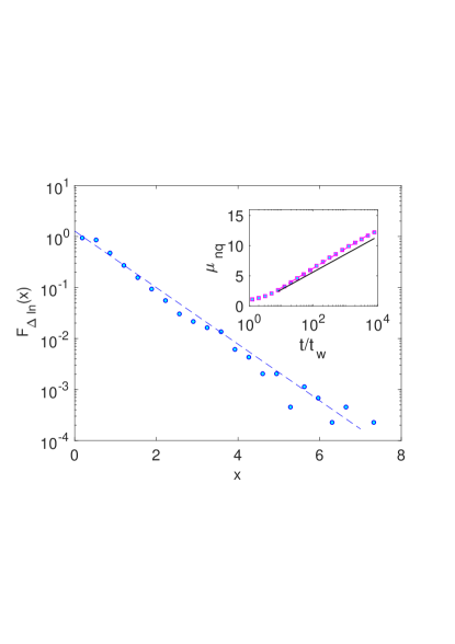
In a large systems, quake to quake correlations, not to be confused with thermal correlations, will eventually die out and temporally close but spatially distant successive quakes will then be uncorrelated. We focus on a spatial domain where quakes are all interdependent, and where the transformation $t\rightarrow\ln t$ captures all temporal correlations. Quaking is then described by a memoryless Poisson process whose average is proportional to the logarithm of time, for short a log-Poisson process.

To ascertain if this is actually the case, it suffices to check whether the log-waiting times between successive events have an exponential PDF with unit average. Log-waiting times are simply defined in terms of the occurrence time $t_{k}$ of the $k$’th quake as $\tau_{k}=\ln(t_{k}/t_{k-1})$. Their empirical PDF is predicted to have the form

$$F_{\rm\Delta ln}(x)=r_{\rm q}e^{-r_{\rm q}x},$$ (4)

where the constant $r_{\rm q}$, the logarithmic quaking rate, is unity. As shown in the main panel of Fig.1, the exponential PDF fits our data, though with a value of $r_{\rm q}$ somewhat higher than predicted. The insert of the same figure shows that the number of quakes that fall in the interval $(0,t]$, averaged over all trajectories, grows as $\mu_{\rm nq}(t)=r^{\prime}_{\rm q}\ln(t)$. The logarithmic growth is as predicted by RD, but $r^{\prime}_{\rm q}>r_{\rm q}$ while $r_{\rm q}=r^{\prime}_{\rm q}$ according to theory. The two lines in the insert of Fig.1 highlight the difference.

To conclude this section, briefly consider the situation where (4) does not fit the empirical distribution of log waiting times. Plainly, the discrepancy can arise if RD does not apply to the problem at hand. The other possibility is that data are collected over a spatial domain large enough to accommodate uncorrelated quakes. In this case the average number of quakes will still grow logarithmically, with a pre-factor reflecting the number of uncorrelated domains contained in the system. Since the waiting time between uncorrelated events is exponentially distributed, once uncorrelated quakes dominate the PDF of waiting times —rather than log-waiting times— between successive quakes will be exponential. To recover Fig. 1 one needs to consider domains of reduced size. Ref. Sibani19 gives an example where this situation arises. Alternatively, one can follow Ref. Boettcher18 and note that uncorrelated quakes produce a peak in $F_{\rm\Delta ln}(x)$ for small waiting times near $x=0$. For sufficiently large $x$, the decay remains unchanged, i.e. exponential.

III.2 Macroscopic data

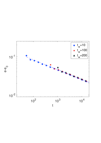
Unlike experiments, numerical simulations provide easy access to the system energy. Figure 2 shows the difference $e(t)-e_{0}$ between the energy per spin and its ground state value plotted vs. time $t$. Three data sets are included, corresponding to different values of $t_{\rm w}$, all three fitted to the same the power law

$$e(t)-e_{0}=at^{\lambda_{e}},$$ (5)

where $e_{0}=-1.6813,\;a=0.2664$ and $\lambda_{e}=-0.2557$ are fitting parameters. As expected, in a linear response experiment, no significant energy dependence appears on the field removal time $t_{\rm w}$.

Equation (5) was proposed in Sibani90a to estimate the ground state energy $e_{0}$ as the value producing the power law decay. The decay was observed in isothermal simulations of the E-A model, using the WTM Sibani07 and parallel tempering Belletti09 . See Eq. (31) and Table 5 of the latter reference for the correspondence to the present notation. These authors tentatively attribute the power law decay to the system being critical for a range of temperatures. Our estimate $e_{0}\approx-1.68$ is nearly identical to that of Sibani07 , while ref. Belletti09 , where much larger systems are considered with two-valued couplings $J_{i,j}=\pm 1$ finds values close to $-1.77$. The exponent $\lambda_{e}$ is a negative and linearly decreasing function of temperature, with the value $\lambda_{e}(T=0.5)\approx-0.25$ from Sibani07 close to our current estimate. Ref. Belletti09 finds $\lambda_{e}(T=0.6)=-0.193$ somewhat higher than our $T=0.5$ value. The mismatch is related to algorithmic details. Note however that Sibani07 and Belletti09 agree on $\lambda_{e}$ being a decreasing function of $T$.

Our main interests lies not in how to best estimate the ground state energy, but in the fact that RD predicts the power law decay, in a way unrelated to critical behavior. Assuming that only quakes can lower the energy, $e(n)$ is a function of the number $n$ of quakes occurring in the interval $(t_{\rm w},t)$. Furthermore, each quake can be expected to decrease the energy difference $\Delta_{e}(n)=e(n)-e_{0}$ by a constant fraction.

Our assumption entails

$$\Delta_{e}(n)=\Delta_{e}(0)x^{n},$$ (6)

$x$, with $0<x<1$. In order to extract a time dependence, the expression must be averaged over the Poisson distribution of the number of quakes falling in the observation interval $(t_{\rm w},t)$ .

Taking $\Delta_{e}(t)=e(t)-e_{0}$, this yields

$$\Delta_{e}(t) = \Delta_{e}(t_{\rm w})\left(\frac{t}{t_{\rm w}}\right)^{-r_{\rm q}}\sum_{n=0}^{\infty}\frac{(xr_{\rm q}\ln(t/t_{\rm w}))^{n}}{n!}$$ (7)

$$= \Delta_{e}(t_{\rm w})\left(\frac{t}{t_{\rm w}}\right)^{-r_{\rm q}(1-x)}.$$

In an RD description, the exponent $\lambda_{e}$ characterizing the energy decay is given by $\lambda_{e}=-r_{\rm q}(1-x)$, which is unrelated to any critical exponent. Power law behavior comes indeed naturally

in processes involving activation over a hierarchy of barriers, see Uhlig95 and references therein.

Figure 2: Symbols: the energy per spin, with a fitted ground state energy value subtracted, is plotted vs. time for three systems with different field removal times. The dotted line is a fit to the power law $y(t)=at^{-\alpha}$, where $a$ and $\alpha$ are free parameters.

Turning now to the Thermoremanent Magnetzation (TRM), we use the gauge transformation $\sigma_{i}\rightarrow\sigma_{i}(t_{{\rm w}})\sigma_{i},\;J_{ij}\rightarrow\sigma_{i}(t_{{\rm w}})\sigma_{j}(t_{{\rm w}})J_{ij}$ to map it into the correlation function

$$C(t_{{\rm w}},t)=\sum_{i}\langle\sigma_{i}(t_{{\rm w}})\sigma_{i}(t)\rangle.$$ (8)

Modulo multiplicative constants, the two functions hold equivalent information and since the general form of the autocorrelation function is theoretically available, we can use it to fit the TRM.

We consider the de-correlation induced by the quakes, which allow the system to equilibrate in increasingly large ergodic components. Quaking is log-time homogeneous stochastic process, involving a set of interacting mesoscopic dichotomic variables, our clusters. Even though a formal description of how clusters interact is lacking, general arguments Sibani13 lead to

$$C(t_{{\rm w}},t)=\sum_{i}w_{i}\exp(\lambda_{i}\ln(t/t_{\rm w})),$$ (9)

where the $\lambda_{i}$s are negative eigenvalues associated to the normal modes of the relaxation process and all $w_{i}$ are positive real numbers.

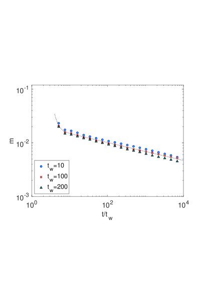
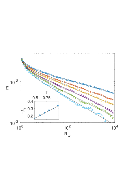
TRM time series are plotted in fig. 3 as symbols vs the scaled time $t/t_{\rm w}$. Neglecting small deviations from pure aging Alba86 , all data are fitted by the same function, represented by a staggered line and obtained by truncating Eq. (9) to two terms, each having the form $w_{i}t^{\lambda_{i}\frac{t}{t_{\rm w}}}$. The fitted exponents are $\lambda_{1}=-0.167$ and $\lambda_{2}=-5.418$ with pre-factors $w_{1}=0.022$ and $w_{2}=30.83$. The first term is well approximated by a logarithm for the range of the abscissa, while the second only matters for values of the latter close to one. Note that power-laws eventually vanish. This ensures that TRM traces with different $t_{\rm w}$ values approach both zero and each other, when plotted as a function of the observation time $t_{\rm obs}=t-t_{\rm w}$. This feature has been measured experimentally Kenning06 , were it was termed ‘end of aging’. Figure 4 shows six TRM traces, taken for $t_{\rm w}=10$ at. temperatures $T=0.5,0.6\ldots 1$, with the staggered line depicting fits based, as before, on Eq. (9). The exponent closest to zero is plotted in the insert vs the temperature $T$, on which it has the linear dependence shown by the line $-\lambda_{1}=0.33T$. . Finally note that our earlier RD analysis of TRM experiments Sibani06 is also based on Eq. (9), but utilizes three rather than two of its terms. The dominant exponent is there closer to zero and almost temperature independent, which produces a near logarithmic TRM decay.

Figure 3: Symbols: Thermoremanent magnetization data for $T=.5$ plotted vs scaled time $t/t_{\rm w}$. Three data sets are shown corresponding to the $t_{\rm w}$ values given in the legend. Dotted line: fit using two terms of the expansion (9).

Figure 4: Symbols: Thermoremanent magnetization data for isothermal aging at temperature $T$. From top to bottom, data sets collected at $T=0.5,0.6,0.7,0.8,0.9$ and $1$ are plotted vs the scaled time $t/t_{\rm w}$, where $t_{\rm w}=10$. Dotted lines: fits using two terms of the expansion (9). Insert: the exponent of the dominant term in the expansion is plotted vs the temperature $T$. The line is the linear fit $-\lambda_{1}=0.33T$.

III.3 Mesoscopic real space properties

The size of thermally correlated domains has attracted both numerical Rieger93 ; Kisker96 ; Sibani94a ; Andersson96 ; Belletti09 ; BaityJesi17 and experimental Joh99 ; Wood10 attention. As the aging process surmounts increasingly high free energy barriers and thermal equilibrium is reached in increasingly larger ergodic components, the domain size is expected to grow. The process has been followed by measuring the correlation length $\xi(t,T)$ associated to the spin-spin correlation function Rieger93 ; Kisker96 , by identifying spatial domains using projections on an alleged ground state obtained by annealing Sibani94a ; Andersson96 , or, experimentally, by an analysis of TRM data introduced by Joh et al. Joh99 . The method follows $S(t_{\rm obs})$, the derivative of the TRM with respect to the logarithm of the observation time, in our notation $t_{\rm obs}=t-t_{\rm w}$, and in particular, the position of its maximum, which demarcates the cross-over at $t_{\rm obs}=t_{\rm w}$ from pseudo-equilibrium to non-equilibrium dynamics. Increasing the applied field reduces the corresponding free energy barriers, and thereby shifts the maximum of $S(t_{\rm obs})$ to the left, by an amount proportional to the size of the spin clusters participating in the barrier crossing process.

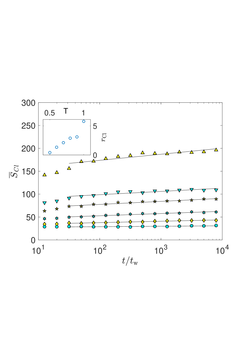
These clusters are observed directly in numerical simulations, here and in Sibani18 , as the coherent movement of adjacent spins triggered by a quake. To obtain the size of clusters flipped ‘near’ a certain time $t$, the simulation time is subdivided into $41$ bins of equal logarithmic duration. Choosing $t$ at the boundary between two bins, all clusters overturned at times within these bins are assigned to $t$.

Figure 5 depicts the average size ${\overline{S}}_{Cl}$ of clusters flipped near time $t$ vs the scaled time variable $t/t_{\rm w}$ for $t_{\rm w}=10$ and temperatures, from top to bottom, $T=1,0.9,0.8,0.7,0.6$ and $0.5$. The lines are fits showing the logarithmic growth of the cluster size, and the corresponding rates are plotted in the insert vs the temperature $T$, The statistics is obtained using 1000 independent simulations for each parameter value. The data can be fitted by the expression

$$S_{\rm Cl}(t,T)=(aT+b)\ln(t/t_{\rm w})+C,$$ (10)

where $a=9.3937$ and $b=-4.44569$ and $C$ is a constant. Clearly, the logarithmic growth rate should never be negative, and our linear fit is inadequate for temperatures below $T=0.5$.

To connect the cluster size to the correlation length $\xi(t,T)$ requires theoretical assumptions Joh99 ; BaityJesi17 which however seem hard to verify unequivocally. The difficulty arises because correlation lengths of all origins, even when observed for long time intervals, only have a modest variation, typically spanning less than a decade. Furthermore, a simple dimensional connection between correlation length and the average size of flipped clusters could be strongly affected by the spatial heterogeneity, since all spins participate in reversible thermal fluctuations, but many are not involved in quakes at all.

Ref.Kisker96 shows that both a power law and a logarithm can fit the time dependence of the correlation length $\xi(t,T)$ for the E-A model of with Gaussian bonds, and Wood10 collects and discusses results from many different sources, all fitted using two power laws, with small exponents linearly dependent on the ratio of the temperature to its critical value.

The time dependence of the cluster sizes extracted from experimental data are shown in Joh99 , on a linear scale vs a logarithmic time scale in their Fig. 4 and on a log-log scale in their Fig.5. Assuming that the characteristic cluster size is the third power of the correlation length $S_{\rm Cl}(t,T)\propto\xi(t,T)^{3}$, the experimental data can be fitted using, for the correlation length, a power law with a small exponent with a linear $T$ dependence, or activated dynamics, i.e a logarithm elevated to a power of order five. Baity-Jesi et al. BaityJesi17 used the same type of analysis as Joh99 to obtain the cluster size from large scale simulations of the $J=\pm 1$ E-A model. They also express the cluster size in terms of a correlation length elevated to a power.

To conclude, our average cluster size features a slow systematic increase with time, that can be fitted by both a logarithm and a power law, in broad agreement with previous findings. The correlation length, on which we do not have direct results, is known to have a qualitatively similar growth. The precise connection between cluster size and correlation length needs, we believe, further numerical verification.

Figure 5: Symbols: the average cluster size ${\overline{S}}_{Cl}$ is plotted vs the scaled time $t/t_{\rm w}$ for different temperatures $T$ and $t_{\rm w}=10$. From top to bottom, the data sets are collected at $T=1,0.9,0.8,0.7,0.6$ and $0.5$. The lines are linear fits of ${\overline{S}}_{Cl}$ to $\log t/t_{\rm w}$. The insert depicts the corresponding logarithmic rates vs the temperature $T$.

IV Summary and Conclusions

Spin glass phenomenology is experimentally well described Nordblad97 ; Vincent07 , while much theoretical understanding relies on partly competing approaches, conceptually rooted in equilibrium statistical mechanics. The ambition of Record Dynamics (RD) is to offer a simple and general coarse-graining method to analyze the dynamics of a class of metastable systems, to which spin glasses belong.

In this work, log-time homogeneity and the ensuing RD predictions for the decay of the excess energy and the TRM are verified in a spin glass thermoremanent magnetization numerical simulation.

In thermal equilibrium, spontaneous fluctuations and linear response convey the same dynamical information, since the initial state of a linear response experiment could also have arisen from a spontaneous fluctuation. The situation is more complicated in a TRM setting, because the barrier structure controlling the dynamics depends on the external magnetic field Joh99 ; Guchhait17 . Barrier climbing has a temperature dependence, described by a temperature scaling exponent. The latter is $\alpha=1$ for the TRM data, as expected from quasi-equilibrium fluctuations, but $\alpha=1.75$ for spontaneous fluctuation, a value explained in Sibani18 in terms of the density of states near local energy minima. Apart from this difference, the present results concur with Ref. Sibani18 . This, combined with the agreement with both experimental and other numerical results, confirms the validity of the WTM as simulational tool.

Finally, we show that the size of spin clusters overturned by quakes grows logarithmically in time, in agreement with Sibani18 . Wood Wood10 collects correlation length data of different origins, and shows that they all can be fitted by a power-law with a small exponent, linearly dependent on the temperature. We doubt that the correlation length and the cluster size have a simple geometric relation. Furthermore, considering that the correlation length typically only varies over less than a decade, the difference between a power law and a logarithm is moot, and the correlation length could well grow logarithmically in time.

To conclude, together with Ref. Sibani18 this work buttresses a RD description of complex dynamics, and confirms that the WTM algorithm, on which our data analysis relies, generates a Markov chain in configuration space which closely mimics the dynamics of experimental systems.