Transitions and Multi-Scaling in Rayliegh-Benard Convection. Small-Scale Universality.

Abstract

Asymptotically large Reynolds number hydrodynamic turbulence is characterized by multi-scaling of moments of velocity increments and spatial derivatives. With decreasing Reynolds number toward $R_{\lambda}=R^{tr}_{\lambda}\approx 9.0$, the anomalous scaling disappears in favor of the ”normal” one and close-to-Gaussian probability densities [Yakhot & Donzis, 119, 044501 (2017)]. The nature of this transition and its universality are subjects of this work. Here we consider Benard convection ( Prandtl number $Pr=1$) between infinite horizontal plates. It is shown that in this system the ”competition” between Bolgiano and Kolmogorov processes, results in small-scale velocity fluctuations driven by effective ”large-scale” Gaussian random temperature field. Therefore, the intermittent dynamics of velocity derivatives are similar or even identical to that in homogeneous and isotropic turbulence generated by the large-scale random forcing. It is shown that low-Rayleigh number instabilities make the problem much more involved and may lead to transition from Gaussian to exponential PDF of the temperature field. The developed mean-field theory yielded dimensional heat flux $Nu\propto Ra^{\beta}$ with $\beta\approx 15/56\approx 0.27$, close to the outcome of Chicago experiment. These results point to an unusual small-scale universality of turbulent flows. It is also shown that at $R_{\lambda}\leq 9.0$, a flow ”remembers” its laminar background and, therefore, cannot be universal.

I Introduction

Transition to turbulence is the series of processes by which a flow passes from regular or laminar to irregular or turbulent as the control parameter, usually the Reynolds number Re, is increased. Formulated this way, transition can be perceived as emergence of chaotic solutions out of deterministic equations of motion as a process of formation, interactions and instabilities of coherent structures. Thus, it is a subject of theory of chaos, pioneered by Lorenz in 1963 who studied instabilities in Benard convection cell Ref.[1]. In this paper we are interested in another kind of transition - the one between two different states of developed turbulence, formulated in [2]-[4].

Transition from laminar to turbulent flow was discovered and analyzed by Osborn Reynolds in 1883, who reported emergence of ”sinuous” motions in steady water flow in a strait pipe. Introducing mean velocity $U\propto\int_{0}^{L}rU(r)dr$, Reynolds quantified the phenomenon in terms of dimensionless parameter $Re=UL/\nu$, later called Reynolds number, so that at $Re\leq Re_{tr}$ the flow was laminar, with a steady parabolic velocity profile $U(r)$. At $Re\geq Re_{tr}$, he noticed appearance of irregular or random fluctuations ${\bf v}({\bf x},t)$ on a laminar background. With increase of $Re>Re_{tr}$, the amplitude and degree of randomness increased which made analysis of the flow very hard. Interestingly, Reynolds was the first to suggest description of this flow using statistical methods of theoretical physics. The transitional Reynolds number $Re_{tr}\approx 2000-14000$, reported in 1883, happened to depend on geometry and quality of the pipe. It has been demonstrated later that in very smooth pipes the flow stayed laminar at least up to $Re_{tr}\approx 10^{5}$ while, depending on degree of wall-roughness, stochastic components in velocity field have been observed at $Re_{tr}\leq 1000$.

One can envision an infinite flow generated by a random force at the scale $L$. If the energy input is sufficiently small, non-linear effects are weak and the system can be described as a large set of almost independent realizations. Therefore, according to CLT, often, it obeys close-to-Gaussian statistics, derived below from dynamic equations. With increase of pumping power, non-linear interactions between the modes grow leading to deviations from Gaussianity which are especially violent at the tails of the probability density functions (PDF) corresponding to the large - amplitude fluctuations. In this paper, we are interested in transitions between weakly and strongly coupled states of a random flow, characterized by different PDF’s.

The magnitude of $Re_{tr}$ can be obtained from solutions to the Navier-Stokes equations with subsequent investigation of their stability. This, in general, very complicated procedure ( for the most recent review see Ref.[1)] is dramatically simplified in the inverse program, introduced below. Since at the scales $r<<L$, turbulence is isotropic and homogeneous, the ”eddies” on the scale $l\approx r$ move with effective velocity Refs.[3]-[4].

$$v_{r,n}=[S_{n}(r)]^{\frac{1}{n}}$$ (1)

Here, the structure functions $S_{n}(r)$ are defined as:

$$S_{n}(r)=\overline{(v_{x}({\bf x})-v_{x}({\bf x}+r{\bf i}))^{n}}\equiv\overline{(\delta_{r}v)^{n}}\equiv\overline{{v_{r}^{n}}}\propto(\frac{r}{L})^{\zeta_{n}}$$ (2)

so that $v_{rms}=v_{r,2}$. Thus, since on the scale $r$ the effective viscosity Ref.[5]:

$$\nu_{r}\approx v_{r}r\approx\sqrt{\overline{v^{2}_{r}}}r$$

the local Reynolds number defied is $Re_{n,r}=v_{r,n}r/\nu$ is a strongly fluctuating flow characteristic which, in some realizations, may be larger than the transitional one. This may lead to appearance of turbulence patches in sub-transitional flows. On the integral scale $\nu_{T}\approx 0.0845{\overline{v^{2}}}^{2}/{\cal E}$ and the effective dynamic or ”dressed” Reynolds number based on Taylor scale is (see Table I) :

$$R_{\lambda}\approx\sqrt{\frac{5}{3{\cal E}\nu_{T}}}v_{rms}^{2}\approx 9.0$$

The result, $R_{\lambda}\approx 10-12$, has been experimentally observed in many engineering setups like flows past bluff bodies like spheres and cars and in numerical simulations of decaying turbulence Ref.[10]. Also, in recent numerical experiments on isotropic and homogeneous turbulence (HIT), driven by different random forces, the transition from the low-Reynolds number Gaussian to strongly anomalous turbulence was found at $R_{\lambda}^{tr}\approx 9.0$, very close $Re_{tr}\approx 8.91$ resulting from the RG -calculations of Refs. [ 6]-[10].

II Multitude of “Reynolds numbers” in a fully developed turbulent flow. Tails and rare events.

Let us identify velocity $v_{r,n}$, defined in (1)-(2) , with velocity of local $n^{th}$-order realization on a scale $r$. Then, in the limit $r/L\ll 1$, the ratio

$$\frac{v_{r,n}(K41)}{v_{r,n}(I)}=(\frac{r}{L})^{\kappa(n)}\rightarrow 0$$

where $\kappa(n)=\frac{3}{4}-\frac{\zeta_{n}}{n}$. Due to intermittency or anomalous scaling, $\zeta_{n}<3n/4$ and, as $n\rightarrow\infty$, $\frac{v_{r,n}(K41)}{v_{r,n}(I)}\rightarrow 0$. Here, $K41$ and $I$ mark the outcomes of Kolmogorov and intermittency theories, respectively. This means that in high Reynolds number flows, at the tails, PDFs of small-scale velocity increments are much ”fatter” than the typical Gaussian PDF, characteristic of K41. Thus, in these not -so-rare flow realizations, corresponding to extreme small-scale fluctuations, the local Reynolds number may be substantially larger than the one based on mild fluctuations with typical velocity $v_{rms}$. In principle, locally, the Reynolds number may be larger than that of transition leading to formation of turbulent patches and dissipative structures.

The moments of derivatives, including those of dissipation rate, ${\cal E}=\nu(\frac{\partial v_{i}}{\partial x_{j}})^{2}$, which are a plausible descriptor of small-scale dynamics, are defined as:

$$M_{2n}=\frac{\overline{(\partial_{x}v_{x})^{2n}}}{{\overline{(\partial_{x}v_{x})^{2}}^{n}}}\propto Re^{\rho_{2n}}$$

where the large-scale Reynolds number $Re$ is defined in Table 1. In the vicinity of transition point we define $v_{rms}\equiv v_{0}$ and the integral and dissipation scales $\eta\approx\lambda$. Multiplying and dividing $M_{2n}$ by $\nu^{n}$ gives:

$$\overline{(\partial_{x}v_{x})^{2n}}=(\frac{v_{0}}{L})^{2n}Re^{2n}={\overline{\cal E}^{n}}\nu^{n}\propto Re^{d_{n}-n}(\frac{v_{0}}{L})^{2n}$$

leading to an important relation [3-[4]]:

$$\rho_{2n}=d_{n}+n$$ (3)

Remarkably, the relatively sharp boundary separating ”anomalous” and ”normal” scalings of velocity derivatives and increments, is very close to $R_{\lambda}\approx 9.-10$. (Ref.[2]-[4]). It has been shown recently that in infinite fluids, stirred by different large-scale random forces, the exponents $d_{n}$ of the moments of dissipation rate:

$$e_{n}=\frac{\overline{{\cal E}^{n}}}{\overline{\cal E}^{n}}\propto Re^{d_{n}}$$

are forcing-independent in the range $R_{\lambda}\geq 9.0-10.0$. In this paper we investigate transition between ”normal” and anomalous flow regimes in Benard convection between two infinite plates heated from below.

It became clear that the so-called Kolmogorov’s scaling $\zeta_{n}=n/3$ and $\rho_{2n}=n$ is not valid for $n\neq 3$ and the moments of orders $m$ and $n$ with $m\neq n$ are given by some ”strange” numbers not related to each other by dimensional considerations. This feature of strong turbulence, called ”anomalous scaling”, is the signature of strong interactions between different modes in non-linear systems. For many years theoretical evaluation of anomalous exponents $\zeta_{n}$ and $\rho_{n}$ was considered one of the main goals of the proverbial ”turbulence problem”. It was shown both theoretically and numerically in Refs.[3]-[4] that possible reason for this difficulty is hidden in the fact that each moment $S_{n}(r)$ and $M_{n}$ should be characterized by its ”own” $n$-dependent Reynolds number $\hat{R}e_{n}$ based on characteristic velocity $\hat{v}(n,n)$, defined in Table 1, and that a widely used parameter $v_{rms}=\hat{v}(2,2)$ is simply one of an infinite number of characteristic velocities describing turbulent flow. The multitude of dynamically relevant Reynolds numbers, necessary for description of turbulence, is defined in Table 1.

Reynolds number	Description
$v_{rms}=\sqrt{\overline{v^{2}}}$	root-mean-square velocity
$\hat{v}(m,n)=\overline{|v|^{m}}^{\frac{1}{n}}$	moment of order $m/n$; $v_{rms}=\hat{v}(2,2)\equiv\hat{v}_{2}$
$Re=v_{rms}L/\nu$	large-scale Reynolds number
$\hat{Re}_{n}=\hat{v}(n,n)L/\nu$	Reynolds number of the $n^{th}$ moment
$R_{\lambda}=v_{rms}\lambda/\nu$	Taylor Reynolds number; $\lambda=15\nu u_{rms}^{2}/{\cal E}$
$Re_{n}^{tr}$	transition point for moments of order $n$
$\hat{R}e_{n}=\hat{v}(n,n)L/\nu$	probes regions with different amplitudes of velocity gradients
$\hat{R}_{\lambda,n}=(5L^{4}/3{\cal E}\nu)^{1/2}\hat{v}(2n,n)$	order-dependent Taylor-scale Reynolds number

Figure 1: Moment-Order-Dependent Transitional Reynolds Numbers. Circles: predicted and numerically tested in Ref.[3]-[4]. Dotted line: numerical simulations of the flow driven by the large-scale random force of Refs. [3]-[4]. Reynolds number of transition decreases with increase of the moment order of $M_{n}$. This explains appearance of turbulence patches/puffs in “sub -transitional” flows.

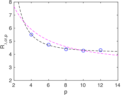
We would like to stress an important point: $v_{rms}$ characterizes typical or relatively mild velocity fluctuations. In general, to be able to predict rare, extreme, events we introduce $\hat{v}_{2n}=L^{2}\overline{(\partial_{x}v_{x})^{2n}}^{\frac{1}{n}}\propto A_{2n}^{\frac{1}{n}}Re^{\frac{\rho_{2n}}{n}}$ and $\hat{R}_{\lambda,n}^{tr}=\sqrt{\frac{5}{{3\cal E}\nu}}\hat{v}_{2n}\approx 8.91$ derived in Refs.[6]-[9]. To calculate large- scale transitional Reynolds number we introduce velocity scale $v_{0}=v_{rms}$ so that $Re=v_{0}L/\nu$ and :

$$\hat{R}_{\lambda,n}^{tr}=\sqrt{\frac{5}{3{\cal E}\nu}}\hat{v}_{2n}=A_{2n}^{\frac{1}{n}}(Re^{tr})^{\frac{\rho_{2n}}{n}+\frac{1}{2}}\approx 8.91$$

It follows from this relation that transition to strong turbulence in different realizations or different-order-moments occurs at a constant $R^{tr}_{\lambda,n}=8.91$ but at different $Re^{tr}=v_{rms}L/\nu$ based on the r.m.s. velocity coming from the second-order moment. This result, theoretically evaluated in [7]-[9], is consistent with the empirical ${\cal K}-{\cal E}$ model giving the large-scale “dressed” viscosity $\nu_{T}=0.0845{\cal K}^{2}/{\cal E}$, used in engineering simulations during last fifty years [6]. Indeed: with ${\cal K}=v_{rms}^{2}/2$

$$R^{tr}_{\lambda}\equiv R^{tr}_{\lambda,2}=\sqrt{\frac{5}{3{\cal E}\nu_{T}}}2{\cal K}\approx 8.88$$

and

$$Re_{n}^{tr}=[\frac{\hat{R}_{\lambda,n}^{tr}}{A_{2n}^{\frac{1}{n}}}]^{\frac{2\rho_{2n}}{2\rho_{2n}+n}}$$

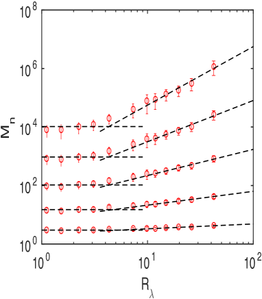
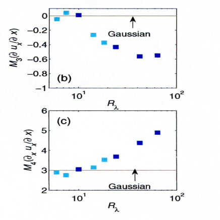
The somewhat “unexpected” but qualitatively reasonable consequence of this result, is seen on Figs.2-3, where the onsets of anomalous scaling for different moments $M_{n}$ are observed at very different $Re_{n}^{tr}$ but at a single $n$-independent $\hat{R}_{\lambda,n}^{tr}\approx 9.0-10$. For large enough $n$, $A_{2n}^{\frac{1}{n}}$ is a weakly dependent function of $n$ which can be calculated from the $Re_{2}^{tr}\approx 9-10$. Thus, one can easily express $Re_{n}^{tr}$ in terms of $\hat{R}_{\lambda,n}^{tr}\approx 9.0-10$ [3] - [4] and close the equation (4) for $\rho_{2n}$. The results are presented in Table II and compared with the data on Fig.1.

III Two examples: flows driven by large-scale external random forces.

In Landau’s theory of ”laminar-to-turbulent transition”, the Reynolds number is defined on a “typical” characteristic velocity $V$ and length-scale $L$ depending on flow geometry, dimensionality, physical mechanisms responsible for instability and other factors characterizing large-scale ordered (laminar) flow. Therefore, in this approach $Re_{tr}$ varies in an extremely wide range of parameter variation. To study dynamics of velocity fluctuations it is useful to define the Reynolds number $Re=v_{rms}L/\nu=\sqrt{\overline{v^{2}}}L/\nu$ based entirely on fluctuating velocity ${\bf v}$ for which $\overline{\bf v}=0$. To avoid difficulties related to instabilities of a laminar flow, we studied the dynamics governed by the Navier-Stokes equations in an infinite fluid stirred by a Gaussian random forcing acting on a finite scale $r\approx L$ Refs. [3]-[4]:

$$\partial_{t}{\bf v}+{\bf v\cdot\nabla v}=-\nabla p+\nu\nabla^{2}{\bf v}+{\bf f}$$ (4)

$\nabla\cdot{\bf v}=0$. Here the density is taken $\rho=1$ without loss of generality. A random Gaussian noise ${\bf f}$ is defined by correlation function:

$$\overline{f_{i}({\bf k},\omega)f_{j}({\bf k^{\prime}},\omega^{\prime})}=(2\pi)^{d+1}D_{0}(k)P_{ij}({\bf k})\delta({\hat{k}+\hat{k}^{\prime}})$$ (5)

where the four-vector $\hat{k}=({\bf k},\omega)$ and projection operator is: $P_{ij}({\bf k})=\delta_{ij}-\frac{k_{i}k_{j}}{k^{2}}$. It is clear from (4)-(5) that in the limit $D_{0}\rightarrow 0$ the nonlinearity is small and ${\bf v}(\hat{k})\approx G^{0}{\bf f}=O(\sqrt{D_{0}})$, where the “bare” Green function is $G^{0}=1/(-i\omega+\nu k^{2})$. In this limit the velocity field is Gaussian with the derivative moments $M_{2n}=\overline{(\partial_{x}v_{x})^{2n}}/\overline{(\partial_{x}v_{x})^{2}}^{n}\approx(2n-1)!!$.

The second example is the one of the Navier-Stokes equations driven by a different forcing mechanism in the rhs of (2) defined as:

$${\bf f}({\bf k},t)=\overline{{\cal E}}\frac{{\bf u}({\bf k},t)}{\sum_{k=1,2}|{\bf u}(\hat{k})|^{2}}\delta_{\bf k,k^{\prime}}$$ (6)

where $\hat{k}=({\bf k},t)$ is a self-consistent solution to the NS equation not equal to zero only at $k_{i}=1;2;$. The advantage of this force is the fixed rate (power) of ”turbulence production” mechanism $\overline{{\bf f}\cdot{\bf u}}=1.0$. The results of numerical simulations are presented on the left and right panels of Fig.2. We see that in both cases transition from Gaussian to anomalous scalings occurs at theoretically predicted $R_{\lambda}\approx 9.0$. In the interval $R_{\lambda,n}>R^{tr}_{\lambda,n}$ numerical simulations gave $M_{2n}\propto R_{\lambda}^{\rho_{n}}$ with anomalous exponents $\rho_{n}$ shown in Table.I. (also see Ref.[2]).

Both examples, considered above, dealt with an infinite fluid stirred at a finite scale $L=O(1)$ . This means that if linear dimension of a fluid is ${\cal L}\rightarrow\infty$, then the flow is generated by $N={\cal L}^{3}/L^{3}\rightarrow\infty$ random, uncorrelated, stirrers, each one defining a statistical realization. Therefore, one can describe a flow either in terms of fluctuations of local parameters or, equivalently, by statistical ensemble with corresponding probability densities (PDFs). This will be demonstrated in detail below.

Figure 2: Left panel: Normalized moments of velocity gradients $M_{2n}$ from direct numerical solutions to the Navier-Stokes equations (4)-(5). At $R_{\lambda}<R^{tr}_{\lambda,n}$ the moments $M_{2n}=(2n-1)!!$, i.e. obey Gaussian statistics. In the range $R_{\lambda,2n}>9.0$, the moments $M_{2n}\propto R_{\lambda}^{\rho_{n}}$, where $\rho_{n}$ are anomalous scaling exponents from Ref. [2]-[4]. Right panel: flow driven by fhe forcing (6) studied in Ref.[2]. The transition from Gaussian to ”anomalous” turbulence at the same $R_{\lambda}\approx 9$ is clearly seen. Sub-gaussian fluctuations in the range $R_{\lambda}<9$ correspond to the more complex low-$R_{\lambda}$ dynamics reflecting complexity of the forcing Ref.[2].

$\rho_{n}$	$GAU$	$DNS$
$\rho_{1}$	$0.46$	$0.455$
$\rho_{3}$	$1.58$	$1.478$
$\rho_{4}$	$2.19$	$2.05$
$\rho_{5}$	$2.82$	$2.66\pm 0.14$
$\rho_{7}$	$4.13$	$3.99\pm 0.65$

Table 1: Comparison of exponents $\rho_{2n}=d_{n}+n$ with the outcome of numerical simulations (DNS) and a theory [3].

$n$	$1$	$2$	$3$	$4$
$R_{\lambda,2n}^{tr}$	$8.91$	$5.5$	$4.8$	$4.5$
$Re_{2n}^{tr}$	$126$	$45$	$35$	$30$

Table 2: Transitional Reynolds numbers based on Taylor scale $R^{tr}_{\lambda,2n}=\sqrt{\frac{5}{3{\cal E}\nu}}v_{rms}^{2}$ of the moments $M_{2n}$. With $\hat{v}_{2}=\overline{v^{2n}}^{\frac{1}{n}}$, the modified Reynolds number $\hat{R}_{\lambda,2n}^{tr}=8.91$ is independent on $n$.

IV Thermal Convection.

The simplified problems of Refs. [2]-[4], described in a previous Section, dealt with transition between a Gaussian state of a fluid and the non-linearity-dominated strong, anomalous, turbulence. In each case, flow was driven by an externally prescribed random force. In real-life -flows, various randomness - generating mechanisms often act simultaneously: for example in wall flows turbulence is produced by instabilities of both quasi-laminar flow patterns in the bulk and those of viscous wall layers, generating powerful bursts reaching into the bulk of a flow. Thus, in this case, the mechanism of transition to anomalous scaling may be much more involved. Below, based on the theory developed in Refs.[12]-[13], we address this problem. The time-dependent number of theoretical, experimental and numerical publications on stability of a fluid heated from below, including Benard convection, is enormous and below we restrict ourselves by quoting only a few necessary sources the derivations are based on.

IV.1 Phenomenology. Reynolds and Rayleigh numbers.

We are interested in a small-scale behavior of a flow between two infinite, thermally insulated, plates separated by the gap $H$. The bottom plate at $z=0$ is heated by an electric current $I$. Sufficiently far from thermal boundary layers, the heat flux averaged over horizontal planes $J_{T}(z)=J(T)=const$ and we keep top and bottom plates under constant temperature difference $T_{top}-T_{bot}\equiv\Delta=const$.

Transition to asymptotic, high Rayleigh number limit, involving formation and transformations of various large-scale coherent structures is an extremely complex process Ref.[1], [14]-[16], [17]-[18]. Detailed study of this fascinating chain of events is beyond the scope of this paper. Here we restrict ourselves to investigation of a few basic steps. First, in the heat conduction range, $Ra=\frac{\alpha gH^{3}\Delta}{\kappa\nu}\leq 1708$, the temperature gradient results in heat flux $J_{T}=\kappa\Delta/H$. In this regime the velocity field ${\bf v}=0$. At $Ra\geq 1708$, the first rolls, contributing to the heat flux, appear on a scale $r\approx H$. In the interval $10^{5}\leq Ra\leq 10^{7}$, according to Busse Ref.[ 15] and Krishnamurti Ref.[14], the flow consists of rolls and hexagonal cells coexisting with imbedded small-scale velocity fluctuations, they call ”convection elements”. These fluctuations exist on the length-scales $r\leq H$. In the interval $Ra>10^{8}$, the instability of boundary layers leads to formation of powerful plumes emitted into the bulk and eventually dominating heat transfer process Ref.[18]. At larger Rayleigh numbers, the fully turbulent flow is dominated by non-linear terms in the equations of motion and in this limit we may expect some kind of universality.

We consider the coupled three-dimensional equations of motion for velocity and temperature fluctuations $v_{i}$ and $T$, respectively:

$$\frac{\partial v_{i}}{\partial t}+v_{j}\frac{\partial v_{i}}{\partial x_{j}} =-\frac{\partial p}{\partial x_{i}}+\nu\frac{\partial^{2}v_{i}}{\partial x_{i}{{}^{2}}}+\alpha gT\delta_{i3}\,,$$ (7)

$$\frac{\partial T}{\partial t}+v_{j}\frac{\partial T}{\partial x_{j}}, =\kappa\frac{\partial^{2}T}{\partial x_{j}^{2}}+\kappa\frac{\partial^{2}\Theta}{\partial x_{j}^{2}}-v_{3}\frac{\partial\Theta}{\partial x_{3}}\,,$$ (8)

Here the horizontally averaged temperature $\Theta=\Theta(z)$ and $\Theta(0)-\Theta(H)=\Delta$. Neglecting compressibility, we set $\partial_{j}v_{j}=0$. Outside thermal boundary $0\leq z\leq l_{B}\equiv l_{d}^{T}$, where both temperature and velocity fluctuations are statistically isotropic field and the mean temperature $\Theta(z)\approx constant$, the heat flux $J_{T}(z)\approx\kappa\frac{\Delta}{l_{B}}\approx const.$. Here $l_{B}$ an approximate thickness of thermal boundary layer which is to be found from equations (7)-(8).

Superficially, the equation (7) looks like equation (4)-(5), considered in Ref.[3]-[4] , but with the forcing ${\bf f}=\alpha gT{\bf k}$, where ${\bf k}(0,0,1)$. This difference is profound: while ${\bf f}$, defined in (5) is, a large-scale Gaussian process, the forcing in e.g..(7) is a solution to dynamic equation (7)-(8). Therefore, first, we would like to investigate temperature fluctuations described by (8). We define:

$$S_{n}(r)\approx\overline{(v(x+r)-v(x))^{n}}\equiv\overline{(\delta_{r}v)^{n}};\hskip 56.9055ptS^{T}_{3}(r)\approx\overline{\delta_{r}v(\delta_{r}T)^{2}}$$

One can easily derive the balance relations:

$$S^{T}_{3}(r)\approx-\frac{4}{3}Nr+\frac{2}{r^{2}}\int_{0}^{r}y^{2}\overline{\delta_{r}v_{3}\delta_{r}T}dy\frac{\partial\Theta}{\partial z}+2\kappa\frac{\partial S^{T}_{2}(r)}{\partial r}$$ (9)

$$S_{3}(r)\approx-\frac{4}{5}\epsilon r+\frac{2\alpha g}{r^{4}}\int_{0}^{r}y^{4}\overline{\delta_{r}v\delta_{r}T}dy+6\nu\frac{\partial S_{2}}{\partial r}$$ (10)

In dimensionless variables: ${\hat{v}}=v/v_{rms};\ {\hat{r}=r/H;\hat{\cal E}=\frac{{\cal E}H}{v_{rms}^{3}}};\hat{N}=\frac{NH^{2}}{\kappa\Delta^{2}}$ with $Ra=\frac{\alpha gH^{3}\Delta}{\nu^{2}}$, the relations (9)- (10) are:

$$\hat{S}_{3}=-\frac{2}{15}\hat{\cal E}\hat{r}+\frac{12}{\hat{r}^{4}}\frac{Ra}{Re^{2}}\int_{0}^{r}\hat{y}^{4}\overline{\delta_{r}\hat{v}\delta_{r}\hat{T}}d\hat{y}+\frac{1}{Re}\frac{\partial\hat{S}_{2}}{\partial\hat{r}}$$

$$\hat{S}^{T}_{3}=-\frac{4}{3}\hat{\cal N}\hat{r}+\frac{2}{\hat{r}^{2}}\int_{0}^{\hat{r}}\hat{y}^{2}\overline{\delta_{r}\hat{v}\delta_{r}\hat{T}}d\hat{y}\frac{\partial\hat{\Theta}}{\partial\hat{z}}+\frac{\partial\hat{S}_{2}}{\partial\hat{r}}$$ (11)

It will be shown below that as $Ra\rightarrow\infty$, the ratio $Ra/Re^{2}\rightarrow\infty$ and $\hat{{\cal E}}=O(1)$ in accord with Kolmogorov relation for isotropic turbulence.

IV.2 Statistical ensemble. Probability Density $P(X)$. Low ”Reynolds Number”.

In an infinite flow driven by externally prescribed large-scale random noise, described by the equations (4)-(6), one deals with a single transition between a Gaussian ($R_{\lambda}\leq R_{\lambda,tr}$) and anomalous ($R_{\lambda}\gg R_{\lambda,tr}$) states. It was shown that, in the two examples discussed above, the transitional parameter $R_{\lambda,tr}\approx 9.0$, independently of the nature of forcing (See Fig.2). This is not a universal statement: in wall flows, in addition to processes happening in the bulk, instabilities of viscous and thermal boundary layers ($z\leq l_{B}$) result in formation of powerful plumes and bursts reaching the bulk and supplying a substantial contribution to the fluxes of kinetic energy and heat. It is clear that geometric details of a cell, like side walls, aspect ratios, curvature play an important part. It will be shown below that each instability of this kind is reflected in the shape of probability distributions functions of temperature and velocity fluctuations. As follows from (7)-(8): $\overline{{\cal E}}=-\alpha g\overline{v_{3}T}$ and our goal is evaluation of all moments $e_{n}=\frac{\overline{{\cal E}^{n}}}{(\overline{(v_{3}T)}^{n}}$. Introducing dimensionless temperature:

$$X=\frac{T^{\prime}}{\Delta}=\frac{V_{pl}\sqrt{\cal E}}{\Delta\sqrt{\nu}\alpha g}=\sqrt{{\cal E}/\overline{{\cal E}}}\equiv\sqrt{e}$$

we would like to evaluate the moments $\overline{X^{2n}}\approx\overline{e^{n}}$.

Below we use a somewhat modified theory of a passive scalar proposed in [11] and applied to the problem of Benard convection in Ref.[12]. Multiplying (8) by $T^{2n-1}$ and, since $\overline{\partial_{j}(v_{j}T^{2n})}=0$, we derive readily:

$$-(2n-1)\overline{T^{2n-2}(\nabla T)^{2}}=\overline{T^{2n-1}v_{3}}\frac{\partial\Theta}{\partial z}$$

With $X^{2}=T^{2}/\overline{T^{2}}$, $Y^{2}=(\nabla T)^{2}/\overline{(\nabla T)^{2}}$ and $W=v_{3}T/\overline{v_{3}T}$. These equations can be rewritten:

$$(2n-1)\overline{X^{2n-2}Y^{2}}=\overline{X^{2n-2}W}$$

and introducing conditional expectation values, gives [10]-[12]:

$$(2n-1)\int X^{2n-2}r_{1}(X)P(X)dX=\int X^{2n-2}r_{3}(X)P(X)dX$$

where

$$r_{1}(X)=\frac{\int Y^{2}(x)\delta(X(x)-X)dx}{\int\delta(X(x)-X)dx}\hskip 56.9055ptr_{3}(X)=\frac{X}{\overline{v_{3}X}}\frac{\int v_{3}(x)\delta(X(x)-X)dx}{\int\delta(X(x)-X)dx}$$

and $r_{1}(X)$ and $r_{3}(X)$ are conditional expectation values of temperature dissipation and production rates for fixed magnitude of dimensional temperature $X$. After simple manipulations, taking into account that at small $X$ production $r_{3}\propto\frac{X^{2}}{\overline{v_{3}X}}$, one obtains a formally exact representation of probability density $P(X)$ [12]-[13]:

$$P(X)=\frac{C}{r_{1}(X)}\exp\big{[}-\int_{0}^{X}\frac{r_{3}(u)du}{ur_{1}(u)}\big{]}=\frac{C}{r_{1}(X)}\exp\big{[}-\int_{0}^{X}\frac{uv_{3}(u)du}{ur_{1}(u)}\big{]}$$ (12)

Interested in the low $Re\leq Re_{tr}\approx 9.0$ limit, we evaluate this expression in the limit $X\rightarrow 0$. First, according to [11]-[12], positive definite conditional dissipation rate

$$r_{1}(X)\approx\alpha+\beta X^{2}=\alpha(1+\frac{\beta}{\alpha}X^{2})$$

Since $v_{3}(T)\approx-v_{3}(-T)$, as $X\rightarrow 0$, we write $v_{3}(X)\approx\gamma X$ and:

$$P(X)=\frac{C}{\alpha}e^{-\frac{\gamma}{2\alpha}X^{2}}$$ (13)

and in the limit $X\rightarrow 0$, the moments of dissipation rate at the center of the cell: $\overline{e^{n}}\approx(2n-1)!!$ similar to the moments of the dissipation rate in isotropic and homogeneous turbulence generated by the large-scale forcing considered in Section III (See Refs.[2],[-4])

Figure 3: Normalized variance (left panel) and third-order moment of the dissipation rate fluctuations (right panel) in the entire interval $Re\geq 10$. In the low $Re\leq Re^{tr}_{n}$ range, the moments $e_{n}$ are equal to $e_{n}=(2n-1)!!$ in accord with (18). The derived transitional $Re^{tr}_{n}$ are presented in Table II. In this case $Re_{pl}\approx 100$, so that $y=0$. The exponents $d_{2}\approx 0.157$ and $d_{3}\approx 0.45$ are found from the matching conditions at $(Re^{tr}_{n})^{d_{n}}=(2n-1)!!$. The results are similar to those in HIT shown on Fig.2.

IV.3 Effect of solid walls and flow instabilities.

In a finite cell, one has to deal with instabilities of boundary layers resulting in formation of plumes emitted into the bulk. Also, formation of ”corner vortices”, fluctuations coming from the side walls and various geometric details may contribute to processes of turbulence production and dissipation. In a general case, denoting critical Reynolds numbers of various instabilities as $R_{pl}^{i}$, we, following Ref.[12], can write an expansion:

$$e\approx X^{2}+\sum y_{i}X$$

where $y_{i}=(Re-Re^{i}_{pl})H(Re-Re^{i}_{pl})$ and $H(x)$ is Heaviside theta function. One can see that, depending on the relative magnitudes of parameters $y_{i}$ and $X$, the heat transfer process is influenced by different instabilities contributing to the ”bumps” in the $Nu(Ra)$ curve, observed in Chicago experiment Ref.[18] . Also, this result agrees with with the recent experimental data by Hong.[16]. Below, to simplify presentation, we consider $i=1$ only and drop the subscript $i$. Thus, the problem is reduced to evaluation of the moments:

$$\overline{e^{n}}=\overline{(X^{2}+yX)^{n}}$$ (14)

Then, since ${\bf v}_{3}\cdot{\bf V}_{pl}>0$, we can write $v_{3}=\gamma X+2yV_{pl}$, where $y=R_{\lambda}-R_{\lambda,pl}\geq 0$ and:

$$\frac{v_{3}(X)}{v_{rms}}\approx\gamma X+2yV_{p}/v_{rms}\approx\gamma X+2\kappa y$$

where $V_{p}/v_{rms}=O(1)$. We can see that when $y=0$, the resulting Gaussian flow is dominated by the weak ”small-scale elements” [14]-[15]. Substituting all this into (12) gives:

$$P(X,y)=\frac{C(y)}{(1+\frac{\beta}{\alpha}X^{2})}\exp[\big{[}-\int_{0}^{X}\frac{\gamma u+2\kappa y}{\alpha(1+\frac{\beta}{\alpha}u^{2})}du\big{]}$$

and the probability density of dimensionless temperature fluctuations at the central part of convection cell with $\alpha=\kappa=1$ is:

$$P(X,y)=\frac{C(y)}{(1+\frac{\beta}{\gamma}X^{2})^{1+\frac{\gamma}{2\beta}}}exp(-2y\arctan(\sqrt{\beta}X)\equiv$$

$$C(y)\Pi(X,y)$$ (15)

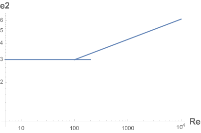
with $C(y)=1/2\int_{0}^{\infty}\Pi(X,y)dX$ and $\beta\approx 1.4$ estimated in [12]. As $y\rightarrow 0$, this expression gives Gaussian PDF with the half-width $\delta\approx\sqrt{\gamma/\beta}$. An interesting feature of this expression is the dependence of the PDF on the Reynolds number $y\neq 0$, consequence of possible instabilities of boundary layers in the range $y>0$ and $R_{\lambda,2}\leq 9.0$. In this range, qualitative dependence of PDF as a function of “Reynolds number” $y$ is shown on Figs.4-5.

IV.4 Moments of dissipation rate. Low-Re regime.

Based on the above derivation (also see Ref.[12]), the conditional expectation value of kinetic energy dissipation rate is approximated by the expression:

$$\frac{\cal{E}}{\overline{\cal E}}\approx yX+X^{2}$$ (16)

and thus, the normalized moments of the dissipation rate are calculated readily

$$e_{n}(y)=\frac{\int_{0}^{\infty}(yX+X^{2})^{2n})P(X,y)dX}{(\int_{0}^{\infty}(yX+X^{2})^{2})P(X,y)dX)^{n}}$$

Figure 4: Probability densities of normalized dissipation rate $e={\cal E}/\overline{\cal E}$ vs ”Reynolds number” $y$.
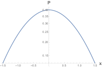
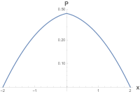
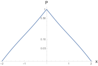
Left panel: $y=0.01$. Middle: $y=0.1$. Right: : $y=1.$. In all cases $\beta=1.4$ as estimated in [12]-[13].

This expression is valid when Reynolds number is so small that the non-linearity in (7) can be neglected, but large enough to allow for the relatively weak boundary layer instability leading to isolated (discrete) plumes.
In the interval $y\ll X$, $yX<X^{2}$ and the probability density $P(X)$ is close to the Gaussian with the first few low-order moments $e_{n}\propto\overline{X^{2n}}\approx(2n-1)!!$.

It is interesting that appearance of two ”Reynolds numbers” $Re$ and $y\propto Re-Re^{tr}$ in (12) , reflects two different mechanisms of turbulence production experimentally observed by Tong et.al. [15]. Indeed, when $y\rightarrow 0$, the length-scale-lacking-fluctuations obey Gaussian statistics. One can also see, that, as the transitional “Reynolds number” $y$ grows, so that $yX>X^{2}$, the PDF (12) varies to close- to -exponential.

IV.5 High Reynolds number limit. Mean-Field theory.

In the limit $Re\rightarrow\infty$ or $\nu\rightarrow 0$ and $\kappa\rightarrow 0$, far enough from thermal boundary layers mean temperature $\Theta\approx const$ and the temperature gradient $\frac{\partial\Theta}{\partial z}$ is very small. Therefore, according to (7)-(10) in dimensionless form:

$$S^{T}_{3}(r)\approx-\frac{4}{3}Nr;\hskip 56.9055ptS_{3}(r)\approx\frac{2\alpha g}{r^{4}}\int_{0}^{r}y^{4}\overline{\delta_{r}v\delta_{r}T}dy$$

A simple approximation, consistent with the mean-field theory developed below:

$$(\delta_{r}v)^{3}\approx 2\alpha g(\delta_{r}v)(\delta_{r}T)$$

gives : $\overline{(\delta_{r}T)^{2}}\propto N^{\frac{4}{5}}g^{-\frac{2}{5}}r^{\frac{2}{5}}$ and $S_{2}(r)\propto g^{\frac{4}{5}}N^{\frac{2}{5}}r^{\frac{6}{5}}$ leading to ”Bolgiano-like” energy spectra:

$$E_{T}(k)\approx N^{\frac{4}{5}}g^{-\frac{2}{5}}k^{-\frac{7}{5}};\hskip 42.67912ptE(k)\approx N^{\frac{2}{5}}g^{\frac{4}{5}}k^{-\frac{11}{5}}$$ (17)

In this paper we consider the relatively simple case of $Pr=\nu/\kappa=1$ and in the mean - field approximation, scale-dependent (”dressed”), transport coefficients, derived in the one-loop renormalized Wild’s diagrammatic expansion gives:

$$\nu(k)=\sqrt{E(k)/k}\approx N^{\frac{1}{5}}g^{\frac{2}{5}}k^{-\frac{8}{5}};$$

In the ”inertial range” of both energy and temperature, the transport coefficients are related: $\nu(k)\approx\kappa(k)$. However in the dissipation range of turbulence $\nu_{T}(k)\rightarrow\kappa$ and at the dissipation scale $\nu(l_{d})\approx\nu=\kappa$

It follows from the above relations that in the inertial range the heat flux is:

$$J_{T}=\nu(k)\int_{0}^{k}k^{2}E_{T}(k)dk=N=const$$

This result means that in this range of scales, heat (temperature) is neither generated nor dissipated. While production mechanism is dominated by convection rolls on the scale $r\approx H$, the heat is dissipated on a scale . $r\leq l_{d}^{T}$, calculated below.

Also, we have from (8)-(9) that at the temperature dissipation scale $l^{T}_{d}$:

$$\frac{4}{3}Nl^{T}_{d}\approx 2\kappa N^{\frac{4}{5}}g^{-\frac{2}{5}}(l^{T}_{d})^{-\frac{3}{5}}$$

and

$$l^{T}_{d}\approx\kappa^{\frac{5}{8}}N^{-\frac{1}{8}}g^{-\frac{1}{4}}$$ (18)

Repeating this calculation for the energy flux $J(k)$, we, using the energy spectrum $E(k)$ from (11), obtain :

$$J(k)=\nu(k)\int_{0}^{k}k^{2}E(k)dk=N^{\frac{3}{5}}g^{\frac{6}{5}}k^{-\frac{4}{5}}$$

In the dissipation range $r<l_{d}^{T}$, the temperature fluctuations are very weak. At the same time, the velocity field, stirred at the scale $r\approx l_{d}^{T}$, is still strong. Indeed, the energy flux $J(k_{i})$ where $k_{i}\approx 1/l_{d}^{T}$, is $O(1)$. Again, using turbulent diffusivity $\nu(k)\approx 0.7\kappa(k)$ applied to the temperature spectrum $E_{T}(k)$, we derive:

$$N=\overline{v_{3}T}[\frac{\partial\Theta}{\partial z}]=\kappa_{T}(\frac{1}{H})[\frac{\partial\Theta}{\partial z}]^{2}=\frac{J_{T}^{2}}{\kappa_{T}(1/H)}\approx J_{T}^{2}g^{\frac{1}{7}}/H^{\frac{6}{7}}$$

where $1/k_{I}\approx H$ is the integral scale.

Since and $g=O(Ra)$ and $N=O(Ra^{\frac{1}{7}})$ we have from (12):

$$H/l_{d}^{T}\approx Nu\approx Ra^{\beta}$$ (19)

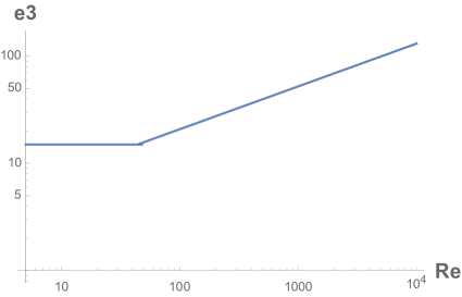
where $\beta\approx 1/4+1/56\approx 0.27$ close to the result of Chicago experiment $\beta\approx 2/7\approx 0.28$ [18]. This result, derived for a particular set up, is in a generally reasonable agreement with experimental data ranging in the interval $0.27\leq\beta\leq 0.3$ with some logarithmic corrections. At this point, the role of aspect ratio, strong intermittency, Prandtl and Rayleigh numbers is hard to assess.

In the temperature dissipation range $r<l_{d}^{T}$ where temperature fluctuations are overdamped, there exist an interval of constant energy flux equal to:

$$J(l_{d}^{T})=N^{\frac{3}{5}}g^{\frac{6}{5}}(l_{d}^{T})^{\frac{4}{5}}\approx g^{\frac{17}{10}}\approx Ra^{\frac{17}{10}}$$ (20)

with Kolmogorov’s energy spectrum:

$$E(k)\approx Ra^{\frac{17}{15}}k^{-\frac{5}{3}}$$

The energy dissipation scale, calculated from the balance $\nu(k)=\sqrt{E(k)/k}=\nu_{0}\propto 1/Re\approx Ra^{-\frac{1}{2}}$ is thus:

$$l_{d}\approx Ra^{-\frac{16}{15}}$$ (21)

From (8) -(11) one derives readily: $Re^{2}=O(v_{rms}^{2})\approx N^{\frac{2}{5}}g^{\frac{4}{5}}\propto Ra^{\frac{6}{7}}$ and $\frac{Ra}{Re^{2}}=O(Ra^{\frac{1}{7}})\rightarrow\infty$ used as an assumption leading to balances (8)-(9). In the limit $Ra\rightarrow\infty$, the relations (11)-(12) give:

$$\frac{l_{d}^{T}}{l_{d}}\approx Ra^{0.797}\rightarrow\infty$$ (22)

As we see, in the temperature dissipation range $r<l_{d}^{T}$, where temperature fluctuations are negligibly weak, there exist an intermediate range

$$l_{d}<<r<<l_{d}^{T}$$

of constant energy flux, given by (20), corresponding to ”Kolmogorov turbulence”. The most important consequence of this result is that in this range the turbulent kinetic energy is produced by the ”large-scale” ($r\approx l_{d}^{T})$ forcing, which is the temperature field of eqs.(7)-(8). The dynamics of velocity derivatives at the scales $l_{d}\ll l_{d}^{T}$, governed by the equations (7)-(8), is reduced to a familiar problem of turbulence driven by the large-scale random force discussed above.

V Summary and discussion. Universality.

Numerical experiments of Refs.[2]-[4] on infinite flows driven by two different large-scale random forces revealed an unexpected transition from a low-Reynolds number Gaussian velocity field to multi-scaling at the Reynolds number $R_{\lambda,2}\approx 8.91$. This, forcing-independent result, hints to a possible non-trivial universality or universality classes of turbulent flows. To test this assumption, in this paper, we study the process of emergence of anomalous scaling in Rayleigh-Benard convection. It is shown that in this system, the temperature field acts as a large-scale stirring force for the velocity field and it has been shown analytically (13) that in the vicinity of transition point $R_{\lambda}\approx 9.0$, this force generates a Gaussian random flow, similar to that in homogeneous and isotropic turbulence of Refs.[2]-[4]. Thus, the anomalous scaling emerges at $R^{tr}_{\lambda,2}\approx 8.91$ calculated in Ref.[6]-[10], in a proximity of a Gaussian field point. While in the high Reynolds number limit $R_{\lambda}\gg 9.0$, all three flows are characterized by the same multi-fractal exponents, they may be very different in the weak-coupling or linear limit $R_{\lambda}<9.0$ . Recently, Das and Girimaji (Ref.[4]), investigating a flow of Refs.[2], discovered a sharp transformation of some geometric flow characteristics at $R_{\lambda}\approx 9.0$, providing a dynamic interpretation of the observed transition.

To study the dependence of a flow on the renormalized (”dressed”) Reynolds number, one can start at $R_{\lambda}\gg 9.0$ and gradually decreasing the Reynolds number toward $R_{\lambda}=R^{tr}_{\lambda}=9.0$, follow emergence of a Gaussian PDF of a temperature field. This gaussian point of turbulence may explain successful one-loop application of Wyld’s renormalized perturbation expansion for derivation of turbulence models widely used for simulation of complex engineering flows.

All above calculations addressed a random flow generated in the central part of the cell, far enough from the wall-boundary layers. According to our assumption, due to efficient mixing, there, $\frac{\partial\Theta}{\partial z}$ is small and, therefore, the heat flux contribution to the balance relation (9) is negligibly small. Corresponding contribution to the balance relation (10) is large, leading to very different energy and heat spectra. This results in heat and energy fluxes operating at widely different length-scales intervals with the energy dissipation scale $l_{d}\ll l^{T}_{d}$. Thus, the temperature field acts as a large-scale stirring force for the velocity field. This brings the small-scale velocity flow in RBC into a class of homogeneous and isotropic turbulence considered in Ref.[2]-[4].

Now, we would like to address Gaussianity of the low-Reynolds number velocity field in the vicinity transition point $R_{\lambda}\approx 9.0$. The representation (12), an exact consequence of equations of motion (7)-(8), is not a closed equation for the PDF $P(X)$. However, in the vicinity of transition point, when $X$ is small enough, the low-order Taylor expansion gives (13) independently of the geometric details. Increasing $X$ or a transition parameter $y$ leads, first, to close-to-exponential and even stretched exponential tails. These features of RBC flow have been predicted in Ref.[12] and experimentally observed in Ref.[15] ,[17].

The mean-field theory, developed above, gave $Nu\approx\frac{H}{l_{d}^{T}}\propto Ra^{\frac{15}{56}}$, close to the result reported in Chicago experiment Ref.[17]. Modern data seem to be closer to $Nu\propto Ra^{\beta}$ with $\beta\approx 0.29-0.31$, with some dependence of exponent $\beta$ on the aspect ratio ${\Gamma}$ and Prandtl number (Pr) (see Ref.[14]). Recently, in a high quality numerical experiments on RBC in a very thin cell ( $\Gamma=d/H=0.1$), K. Iyer, et.al. ( Ref.[16]), reported $\beta=0.331$, very close to a classic exponent derived by Malcus in 1954 (Ref.18]). With increase of the aspect ratio $\Gamma$, the observed exponent was in the range $\beta\approx 0.28-0.30$ Ref.[14]. The present mean-field theory was developed for the flow in a cell of $\Gamma\rightarrow\infty$ which may, after all, be close to the asymptotic limit $\beta\approx 2/7$. It still remains to be seen.

It has to be stressed that in this work no effects of intermittency have been accounted for as well as the role of Prandtl number, aspect ratio, instabilities of side walls boundary layers which, in principle, can explain the small difference between our mean-field theory and experimental data. Another possibility is much more exciting: according to the developed above theory, the transition point $R_{\lambda}\approx 8.91$ is Gaussian, which may explain validity of the mean-field approximation and $\beta\approx 15/56$ in a flow between infinite plates and $Pr=1$, which is beyond present-day experimental setups. Today, this suggestion can be considered as a mere speculation.

References

- (1) A.M. Yaglom, Hydrodynamic Instability and Transition to Turbulence, Springer, ,2012; L.E.Lorenz, “Deterministic nonperiodic flow”, J.Atmos.Sci. 20, 130-141 (1963 ).
- (2) J. Schumacher, K. R. Sreenivasan, and V. Yakhot, New J. Phys. 9, 89 (2007).
- (3) V. Yakhot and D. A. Donzis, Phys. Rev. Lett. 119, 044501, (2017)
- (4) V. Yakhot and D. A. Donzis, PhysicaD. xx, 044501 (2018); R.Das and S.Girimaji, “On the Reynolds number dependence of velocity structure and dynamics,” J.Fluid.Mech. 2018 (in press)).
- (5) L. D. Landau and E. M. Lifshitz, Course of Theoretical Physics, Statistical Physics, Volume 5, Butterworth-Heinemann, Oxford, 1980.
- (6) B.E. Launder and D.B. Spalding, “Mathematical Models of Turbulence”, Academic Press, New York (1972); In turbulence modeling literature model is used with experimentally determined coefficient instead of the derived .
- (7) V. Yakhot and L. Smith, “The renormalization group, the -expansion and derivation of turbulence models”, J. Sci. Comp. 7, 35 (1992).
- (8) V. Yakhot, “Reynolds number of transition and self-organized criticality of strong turbulence”, Phys. Rev. E,90, 043019 (2014).
- (9) V. Yakhot, S.A. Orszag, T. Gatski, S. Thangam and C. Speciale, “Development of turbulence models for shear flows by a double expansion technique”, Phys. Fluids A4, 1510 (1992);
- (10) V.Borue, S.A. .Orszag, “Local energy flux and subgrid-scale statistics in three-dimensional turbulence.” J.Fluid.Mech, 366,1,(1998)
- (11) Ya.G. Sinai, and V. Yakhot, Phys. Rev. Lett. 63, 1965 (1989). V. Yakhot, Phys. Rev. Lett. 63, 1965 (1989).
- (12) V. Yakhot, S. A. Orszag, S. Balachandar, E. Jackson, Z.-S. She, and L. Sirovich, J. Sci. Comput. 5 (3), 199 (1990).
- (13) R. Krishnamurti, J . Fluid Mech. 33 457-631970a; J. Fluid Mech. 42 295-307 1970b;
- (14) Busse, F. H., Non-linear properties of thermal convection 1978 Rep. Prog. Phys. 41 1929 p.1943;
- (15) X.He and P.Tong, “Measurements of thermal dissipation field in Benard convection” Phys.Rev.E,79,026306 (2009)
- (16) Kartik P.Iyer, J.D.Scheel, J. Schumacher and K.R.Sreenivasan, “Classical 1/3 scaling of convection holds up to ” PNAS, (2020))
- (17) B. Castaing, G. Gunaratne, F. Heslot, L. P. Kadanoff, A. Libchaber, S. Thomae, X.-Z. Wu, S. Zaleski, G. Zanetti, J. Fluid Mech. 204, 1 (1989).
- (18) W. V. R. Malkus, Proc. R. Soc. Lond. A 225, 185 (1954).