Dynamic symmetry-breaking in mutually annihilating fluids with selective interfaces

Abstract

The selective entrapment of mutually annihilating species within a phase-changing carrier fluid is explored by both analytical and numerical means. The model takes full account of the dynamic heterogeneity which arises as a result of the coupling between hydrodynamic transport, dynamic phase-transitions and chemical reactions between the participating species, in the presence of a selective droplet interface. Special attention is paid to the dynamic symmetry breaking between the mass of the two species entrapped within the expanding droplet as a function of time. It is found that selective sources are much more effective symmetry breakers than selective diffusion. The present study may be of interest for a broad variety of advection-diffusion-reaction phenomena with selective fluid interfaces.

1 Introduction

The spatial dynamics of mutually annihilating species is a subject of wide interdisciplinary concern, with many applications in chemistry, condensed matter, material science and even cosmology, with the famous problem of baryogenesis, namely the large asymmetry between matter and antimatter observed in the current Universe [7, 2].

A pioneering investigation by Toussaint and Wilczek [20], pointed out that the time asymptotic behaviour of the mutually annihilating species ($A$ and $B$ for convenience) crucially depends on the initial conditions. The rationale is quite intuitive: if the species mix, they react and both disappear according to the irreversible reaction $A+B\to P$, where $P$ denotes a set of product species which contains neither $A$ nor $B$. If, on the other hand, by some transport mechanism, they manage to demix or segregate apart, so that the product of their concentrations becomes vanishingly small, then annihilation is quenched, thus spawning a chance for both species to survive much longer than under homogeneous mixing conditions.

Besides being of great interest on their own right, the details of such survival may have plenty of applications in chemistry, material science or biology, an example in point being the absorption of drugs within liquid droplets for microfluidics and drug-delivery applications [21, 4, 10, 13].

In this paper we consider a specific mechanism of segregation associated with the growth of droplets within a phase-changing carrier fluid. By postulating a selective transport of the two species across the droplet interface (membrane), we introduce a symmetry-breaking mechanism which is ultimately responsible for the differential entrapment of the facilitated species (the one with higher transmissivity across the membrane, say $A$) with respect to the inhibited one (say $B$). The practical question is: how much mass of both species is entrapped in the growing and moving droplet as a function of time? Once again, this is interesting per-se as a fundamental transport problem in dynamically heterogeneous media, and also for the aforementioned practical purposes. To the best of our knowledge, no detailed account of the hydrodynamic complexity associated with a moving and expanding droplet, in the presence of transport and chemical reaction, has ever been discussed. This is precisely the aim of the present work, with prospective focus on electroweak baryogenesis.

2 The transport model

We consider three species $A$, $B$ and $C$, where $C$ is a fluid carrier undergoing phase-changes, while $A$ and $B$ are passively transported by $C$ and mutually annihilate through chemical reactions.

The three species $k=1,2,3$ obey a continuity equation of the form [6]

$$\partial_{t}\rho_{k}+\partial_{a}(\rho_{k}\ u_{k,a})=r_{k}+s_{k}$$ (1)

where $a=x,y,z$ runs over spatial dimensions and obeys Einstein’s summation rule.

In the above $r_{k}$ and $s_{k}$ denote the density change rate due to chemical reactions and generic sources, respectively.

Species $A$ and $B$ share the same mass, which we set to unity by convention, $m_{A}=m_{B}=1$, so that the number and the mass of the species are the same quantity.

The two species annihilate at the following rate:

$$r_{A}=r_{B}=-\alpha\rho_{A}\rho_{B}$$ (2)

where $\alpha$ is an adjustable reaction parameter.

The $C$ field serves as a carrier for the $A$ and $B$ species and obeys a non-ideal Navier-Stokes equation:

$$\partial_{t}(\rho_{C}\ u_{a})+\partial_{b}P_{C,ab}=s_{C}$$ (3)

where

$$P_{C,ab}=\rho_{C}\ u_{a}u_{b}+p_{C}\delta_{ab}-\sigma_{ab}+\chi\partial_{a}\rho_{C}\partial_{b}\rho_{C}$$ (4)

is the non-ideal momentum flux tensor, including the contributions of inertia, ideal and non-ideal pressure, dissipation and the capillary forces responsible for the first-order phase transition. The term $s_{C}$ represents an external source of mass.

Species $A$ and $B$ are passively transported by the $C$-field and diffuse across it with diffusivity coefficients $D_{A}$ and $D_{B}$ respectively.

The $A$ and $B$ species experience a selective permeability of the droplet interface, so that an excess of $A$ over $B$ accumulates around the interface and further penetrates within the expanding droplet.

The actual amount of mass engulfed within the droplet resulting from such complex transport process is highly sensitive to the chemical details, as well as to the hydrodynamic evolution of the system.

Our main aim is to investigate the complex transport phenomena which result from the dynamic competition between advection, diffusion and reaction processes taking place in the framework of a phase-changing carrier fluid.

In our stylized model, microscopic symmetry breaking between species $A$ and $B$ is accounted for by two mechanisms: i) different values of the diffusivities and ii) different source terms, for species $A$ and $B$, respectively.

2.1 Selective diffusivity

The diffusion coefficients are taken in the form:

$$D_{k}(\rho)=D_{k}^{in}\theta(\rho-\rho_{m})+D_{k}^{out}\theta(\rho_{m}-\rho),\;\;\;k=A,B$$ (5)

where $\rho_{m}=(\rho_{l}+\rho_{v})/2$ is the mean carrier density within (liquid) and outside (vapour) the droplet, while $\theta(x)$ is the Heavyside step function. Smoother versions can easily be implemented, but in this work we shall stay with the discontinuous model.

The $AB$ symmetry-breaking processes are accounted for by choosing a different ratio between the inner (within the droplet) and outer (outside the droplet) diffusion coefficients of the $A$ and $B$ species, namely, $J_{A}\neq J_{B}$, where we have defined the in-out diffusion jump factors as:

$$J_{k}\equiv\frac{D_{k}^{in}}{D_{k}^{out}},\;k=A,B$$ (6)

For convenience, we set the same outer diffusivity for species $A$ and $B$, namely:

$$D_{A}^{out}=D_{B}^{out}=D$$ (7)

In particular, we note that $J<1$, i.e. smaller diffusivity inside the droplet than outside, implies a net flux towards the interface, due to the diffusive velocity $\vec{u}_{D}=-\nabla D$. This is consistent with the fact that diffusivity is supposed to decrease at increasing carrier density.

2.2 Selective sources

We shall consider the following source terms

$$s_{A}(x,y)=s_{0}W(\vec{r}-\vec{r}_{s})$$ (8)

$$s_{B}(x,y)=\zeta s_{0}W(\vec{r}-\vec{r}_{s})$$ (9)

where $W(\vec{x})$ is a piece-wise constant centred around the droplet interface, and $0\leq\zeta\leq 1$ is the symmetry-breaking parameter. Such source term models the effect of catalytic reactions acting at the droplet surface, although we shall not delve into any detail of their specific origin.

3 Numerical set-up

The transport equations described above are solved by means of a three-species lattice Boltzmann (LB) scheme [19, 1, 8, 5] (see Appendix). The main reason for using LB is its ability of dealing with dynamic phase-transitions in a much handier way than solving the Navier-Stokes equations of non-ideal fluids.

In the sequel, we introduce the simulation set-up and present numerical results for both the selective scenarios described in the previous section.

We consider a two-dimensional square with $L=1024$ grid-points per side and run the simulations over a timespan of $10^{6}$ time-steps, thus covering three decades in space and six in time, as it is appropriate for diffusive phenomena.

3.1 Initial and boundary conditions

Both species are initialised at the same constant density value throughout the computational domain:

$$\rho_{A}(x,y)=\rho_{B}(x,y)=\rho_{0}=1$$ (10)

The initial density of the carrier field is defined as follows:

$$\rho_{C}(x,y)=\rho_{in}(1\pm\eta),\;\ R_{0}$$ in a ball of radius (11)

$$\rho_{C}(x,y)=\rho_{out},\;$$ outside the ball (12)

where $\eta$ is a zero-mean random perturbation with rms $\delta\rho/\rho=0.01$.

We take $\rho_{0}=1$, $\rho_{in}=0.2$, $\rho_{out}=0.10$ and $R_{0}=10$.

For the phase transition, we choose $T/T_{c}=0.04/0.047$, corresponding to a coexistence liquid/vapour density ratio of about $0.27/0.027=10$.

The values of $\rho_{out}$ and $\rho_{in}$ determine the duration of the growth stage, i.e. the time it takes for the droplet to attain the coexistence values of the liquid ($l$) and vapour ($v$) phases.

By mass conservation:

$$\rho_{in}V_{in}+\rho_{out}V_{out}=\rho_{l}V_{l}+\rho_{v}V_{v}=M$$ (13)

where $V_{in}+V_{out}=V_{l}+V_{v}=V=L^{2}$ is the total volume of the system in two dimensions.

Clearly, the volume of the droplet grows at increasing the total mass in the system. More specifically, the final value of the volume fraction, i.e. the ratio of the volume of the liquid droplet to the total volume, is given by:

$$\lambda\equiv\frac{V_{l}}{V}=\frac{\rho_{m}-\rho_{v}}{\rho_{l}-\rho_{v}}$$ (14)

where $\rho_{m}=M/V$ is the average mass density.

The diameter of the liquid droplet is thus given by:

$$D=L\sqrt{\frac{4}{\pi}\lambda}$$ (15)

Hence, the maximum droplet diameter, $D=L$, is attained at the a volume fraction $\lambda_{max}=\pi/4\sim 0.78$.

Finally, all species are taken initially at rest, namely:

$$\vec{u}_{k}(x,y)=0,\;k=A,B,C$$ (16)

Full periodicity is assumed across the four boundaries of the simulation box.

3.2 Chemical rates and diffusivities

Collisional time-scales are fixed at $\tau_{A}=\tau_{B}=\tau_{C}=1$, which is the fastest timescale in action. This corresponds to an outer diffusivity and carrier viscosity, $D_{A}=D_{B}=\nu_{C}=1/6$ in lattice units (see Appendix).

The annihilation rate is taken as $\alpha=0.1$, corresponding to an annihilation timescale $\tau_{a}=10$ at unit density $\rho_{k}=1$.

The diffusion timescale across the membrane is $\tau_{d}=w^{2}/D$, $w$ being the width of the droplet interface. Given that in LB simulations $w\sim 5$ lattice units, this corresponds to a Damkohler number (diffusive/chemical timescale), $Da\equiv\tau_{d}/\tau_{a}\sim 15$. This means, at unit density, annihilation is about $15$ times faster than the diffusive time scale, which also means that annihilation is effective within the droplet interface. At densities below $1/15$ the two time scales become comparable, and the interface becomes chemically transparent.

4 Analytical considerations

To gain perspective, it is of interest to analyse the homogeneous case, which proves amenable to some analytical considerations. In the homogeneous-symmetric scenario $D_{A}=D_{B}=0$, no-phase transitions, no sources and symmetric initial conditions, both species decay according to the nonlinear homogeneous equation:

$$\frac{d\rho_{k}}{dt}=-\alpha\rho_{k}^{2}$$ (17)

whose analytical solution reads as follows:

$$\rho_{k}(t)=\frac{\rho_{k0}}{1+\alpha\ \rho_{k0}\ t},\;k=A,B$$ (18)

This yields a $\tau_{k}/t$ decay, where

$$\tau_{k}\equiv\frac{1}{\alpha\ \rho_{k0}},\;k=A,B$$ (19)

is the density-dependent annihilation time-scale.

In the presence of a symmetry-breaking membrane, the two species are expected to develop different values of $\tau_{k}$, which we refer as to a dynamic symmetry breaking, due to the effect of the selective interface on the species density. Such dynamic symmetry breaking is expected to occur as soon as the droplet starts to grow, i.e. it starts to nucleate out of its initial seed of radius $R_{0}$. Both species $A$ and $B$ begin to be entrapped within the nucleating droplet and their mass within the droplet grows accordingly, as long as the droplet growth rate exceeds their annihilation rate.

As we shall see, such growth is far from monotonic, but characterized instead by large fluctuations, due to the carrier density waves radiating away from the expanding droplet. Such oscillations do not settle down until the droplet condensation has come to an end, i.e at $t\sim\tau_{con}\equiv R/\dot{R}$, where $\tau_{con}$ defines the condensation time of the droplet, i.e. the time it takes for its mass to reach steady-state.

In the long-term, namely at $t\gg\tau_{con}$, the densities of the two species are expected to settle to constant values inside and outside the droplet, thus leading to the coexistence of two homogeneous compartments: the droplet and its surrounding environment.

Since the droplet is homogeneous, the mass of the entrapped species is expected to follow again a $\tau_{k}/t$ decay, with two different values of $\tau_{A}$ and $\tau_{B}$, due to the aforementioned dynamic symmetry breaking.

In the sequel, we shall put these qualitative considerations on quantitative grounds based on the result of extensive numerical simulations.

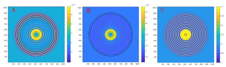
Figure 1: Color plates of the density of the species A, B and C during the growth stage. Density/pressure waves radiating away from the droplet are clearly visible.

5 Numerical Results: Selective Diffusion

We consider the source-free case $s_{A}=s_{B}=0$ and define a quantitative symmetry-breaking indicator in the form of the diffusivity jump factor, $J_{AB}=J_{B}/J_{A}$.

We run three representative cases: $J_{AB}=0.01,0.1,1$, the latter denoting the unbroken, symmetric case.

For the parameters in point, namely $R_{0}=10$, $\rho_{in}=0.2$, $\rho_{out}=0.1$, the total initial mass of the carrier fluid is $M_{C}(0)=0.2\ \pi\ 10^{2}+0.1\ (1024^{2}-\pi\ 10^{2})\sim 10^{5}$, hence the initial carrier density is $\rho_{m}\sim 0.1$. With $\rho_{l}=0.27$ and $\rho_{v}=0.027$, as dictated by the equation of state, we obtain $\lambda\sim 0.61$, which gives a final droplet volume of about $6\cdot 10^{5}$ lattice units, corresponding to a diameter $D\sim 900$ lattice units, pretty close to the maximum value that can be attained on a lattice of side $L=1024$ lattice units.

The initial value of the masses is $M_{A}(0)=M_{B}(0)=1024^{2}\sim 10^{6}$, of which only $100\pi\sim 314$ lies inside the initial seed droplet.

For the present parameters, the droplet is found to reach its final size, $D\sim 900$ lattice units, after about $\tau_{con}\sim 1.2\;10^{4}$ steps, corresponding to an average growth rate $\dot{R}\sim(R_{f}-R_{0})/\tau_{con}\sim(450-10)/1.210^{4}\sim 0.04$, significantly slower than the sound speed, $c_{s}=1/\sqrt{3}$, both in lattice units. This implies that the during the growth stage, the expanding droplet emanates trains of density waves radiating away from it. As we shall see, such density waves are well visible in the simulations.

In Fig.3 we report the time evolution of the mass $A$, $B$ and $C$ within the droplet, as well as the order (phase-field) parameter:

$$\phi_{AB}\equiv\frac{M_{A}-M_{B}}{M_{A}+M_{B}},$$ (20)

which provides a direct measure of symmetry breaking. Indeed, by definition, $\phi_{AB}=0$ under symmetric conditions, while $\phi_{AB}=\pm 1$ in the full $A$($B$) components, respectively.

As one can see, after a short-term transient, in which both species decrease due to annihilation, the $A$ and $B$ masses start to increase, due to the entrapment within the growing droplet. At about $t\sim 10^{3}$, large oscillations start to take place, due to the radiation of density(pressure) waves from the growing droplet, which lead to local condensation and subsequent evaporation of annular rings around the droplet. These rings are well visible in the three snapshots of the carrier density contours, as reported in the lower insets of panel (a,b), corresponding to three distinct time instants.

It is interesting to notice that in the regime of wild oscillations, the species $B$ eventually exceeds species $A$, which we tentatively interpret as a dynamic effect of the presence of the rings.

Panel b) reports the long-term evolution of the three masses $A$,$B$,$C$, in the time frame $10^{3}<t<10^{6}$. The main result is that the facilitated species $A$ prevails over $B$, but only by a comparatively small amount. Indeed, the largest value attained by the order parameter was $0.27$ for the case $J_{AB}=0.01$. Once the droplet settles down, both species start to decay according to the homogeneous rate $1/t$, although with a slightly different amplitude, due to the dynamic symmetric breaking which occurred in the condensation stage.

The density contours of species $C$ highlight that the equilibrium spherical shape is reached by the droplet after a very long time-span. Notwithstanding the major shape changes, $C$ mass remains constant, and this is sufficient for the homogeneous decay $1/t$ to settle down, long before the droplet attains mechanical equilibrium.

Finite-size effects are also visible, through the reflection of density waves at the boundary. Indeed, since we work at pretty large values of geometric confinement, $D/L\sim 0.9$, such boundary effects are inevitable.

In all the considered cases, symmetry breaking remains comparatively small at all times, notwithstanding the large values of the jump coefficients used in the simulations.

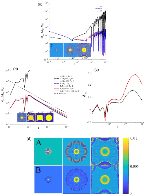
Figure 2: Time evolution of the masses of species $A$, $B$ and $C$ inside the droplet, short term (a) and long term (b) for the cases $J_{AB}=0.01$ and $J_{AB}=0.1$ (see legend). The dashed line in panel (b) is a eye-guiding fit $10^{7}/t$. In panel (c) we report the long term evolution of the order parameter $\phi_{ab}$ for the cases $J_{AB}=0.01$ (top) and $J_{AB}=0.1$ (bottom). The inset in panel (b) reports snapshots of the density contours of the carrier species $C$, while the density contours of species $A$ and $B$ are reported in panel (d).

6 Numerical Results: Selective Sources

In this section, we investigate the effects of selective source terms for the species $A$ and $B$, by changing the asymmetry source coefficient in the range $0.4\leq\zeta\leq 1$.

The other main parameters are the same as in the previous simulations, except for $D_{A}=1,D_{B}=1$ and $s_{0}=10^{-3}$.

In Figure 3, we present the time evolution of the mass of species $A$, $B$ and $C$ within the droplet, for the case $\zeta=0.99$.

The short-term behaviour is similar to the case of selective diffusion, although a more substantial symmetric breaking between the $A$ and $B$ masses is observed.

As clearly shown in panel 3(b), the main difference is the neat separation in the long run, due to the fact that any symmetry breaking of the source terms leads a secular growth of the facilitated species, $M_{A}(t)\sim a\ t$, versus a homogeneous $b/t$ decay of the unfacilitated one, as we shall discuss shortly.

As a result, the mass ratio goes to zero like $t^{-2}$.

Similarly to the case of selective diffusion, the time asymptotic behaviour sets in long before the density configuration in space reaches its mechanical equilibrium, the chief condition being that the mass of the droplet be stationary in time, regardless of its shape.

Since the majority species follows a linear trend $M_{A}(t)\sim t$, while the minority one obeys a reciprocal trend $M_{B}(t)\sim 1/t$, their product remains basically asymptotically constant in time, which is indeed confirmed by the numerical results.

As we shall show in the next section, these results can be interpreted in terms of analytical solutions of the homogeneous driven case.

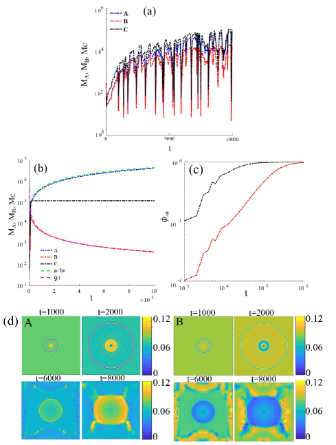
Figure 3: Short (a) and long (b) time evolution of the masses of species $A$, $B$ and $C$ inside the droplet for the case of selective sources with $\zeta=0.99$. Panel (c) reports the order parameter $\phi_{AB}$ as a function of time for the cases $\zeta=0.99$ (bottom) and $\zeta=0.999$ (top). Panel (d) reports four snapshots of the density contours of species $A$ (left) and $B$ (right) for the case $\zeta=0.99$.

6.1 Homogeneous driven case: analytical model

The equations of the mass evolution within the droplet for the homogeneous (no diffusive fluxes) driven system read as follows:

$$\dot{M}_{A}=-\alpha R_{AB}+S_{A}$$ (21)

$$\dot{M}_{B}=-\alpha R_{AB}+S_{B}$$ (22)

where we have defined the global density overlap $R_{AB}=\int\rho_{A}(x,y)\rho_{B}(x,y)dxdy$, and the global mass inputs per unit time, $S_{k}=\int s_{k}(x,y)dxdy$, $k=A,B$.

Subtracting the two equations (21), delivers:

$$\dot{M}_{A}-\dot{M}_{B}=S_{A}-S_{B},$$ (23)

which shows that the mass deficit $M_{A}-M_{B}$ grows linearly in time.

By multiplying the first by $M_{B}$, the second by $M_{A}$ and summing them up, we obtain

$$\frac{d}{dt}(M_{A}M_{B})=-\alpha R_{AB}(M_{A}+M_{B})+S_{B}M_{A}+S_{A}M_{B}$$ (24)

Assuming $M_{B}$ to decay asymptotically to zero, the right hand side is made zero by imposing

$$R_{AB}\sim\frac{S_{B}}{\alpha}$$ (25)

Next, we write $R_{AB}=\xi_{AB}\frac{M_{A}M_{B}}{V_{C}}$, which defines $\xi_{AB}$ as the spatial correlation coefficient, $V_{C}$ being the droplet volume.

Further expressing the density as a volume average plus a spatial fluctuation, $\rho_{k}=M_{k}/V_{C}+\tilde{\rho}_{k}$, and assuming weak spatial fluctuations, $\tilde{\rho}_{k}V_{C}/M\ll 1$, the correlation coefficient is made $1$. Thus, the expression (25) finally yields:

$$M_{A}M_{B}=\frac{S_{B}V_{C}}{\alpha}=Const.$$ (26)

As anticipated earlier on, this is indeed found to be consistent with the numerical observations.

Summarizing, the time-asymptotic behaviour of the engulfed masses is given by:

$$M_{A}(t)\sim(S_{A}-S_{B})t$$ (27)

and

$$M_{B}(t)\sim\frac{S_{B}V_{C}}{\alpha M_{A}(t)}.$$ (28)

One can solve explicitly also for the non-asymptotic regime, to obtain:

$$M_{A}(t)=s_{0}V_{s}\frac{(1-\zeta)t}{2}(\sqrt{1+4\tau^{2}/t^{2}}+1)$$ (29)

$$M_{B}(t)=s_{0}V_{s}\frac{(1-\zeta)t}{2}(\sqrt{1+4\tau^{2}/t^{2}}-1)$$ (30)

where $V_{s}=\pi Dw$ is the shell volume around the interface.

In the above, we have set

$$\tau=\tau_{s}\;\frac{\zeta^{1/2}}{1-\zeta}$$ (31)

with $\tau_{s}\equiv 1/(\alpha s_{0})$. For the current simulations, $\tau_{s}=10^{4}$, fairly close to the droplet equilibration time, $\tau_{con}\sim 1.2\;10^{4}$.

The upshot of the above analysis is that the majority species grows asymptotically like $(1-\zeta)t$ and the minority species decreases like $\zeta/t$. As a result, the mass ratio $M_{A}/M_{B}$ grows quadratically unbounded in time.

This is potentially far reaching, since it means that even a minuscule asymmetry in the sources is destined to give rise to the extinction of the minority species on a times scale proportional to $\zeta^{1/2}/(1-\zeta)$, which clearly diverges in the symmetric limit $\zeta\to 1$. In this limit, $M_{A}=M_{B}=\sqrt{\frac{S_{B}V_{C}}{\alpha}}$.

A similar treatment goes for the non-homogeneous case, provided the source terms are augmented with the corresponding diffusive fluxes.

7 Prospects for electro-weak baryogenesis

The results presented so far indicate that selective diffusivity is a weak symmetry breaker, whereas selective sources are way more effective.

It is therefore of interest to speculate whether the present model can be of any use in the context of electro-weak baryogenesis (EWBG) [14].

To this purpose, let us remind that, so far, we referred to $A$ and $B$ as generic mutually annihilating species carried by a phase-changing fluid $C$.
Baryogenesis implies the identification

• $A$ = matter

• $B$ = antimatter

• $C$ = Higgs field

Although we refrain from making any claim of quantitative relevance to EWBG, it is nonetheless of interest to assess the plausibility of present model towards the basic requirements laid down by Sakharov, back in the mid sixties [16].

They amount to the following three basic conditions:

• i) The existence of an explicit baryon-symmetry breaking mechanism,

• ii) Violation of C and CP invariance,

• iii) Thermodynamic non-equilibrium

As to i), the baryon symmetry breaking is expressed by the non-unit diffusion jump factor $J_{AB}$ across the membrane, or an explicit symmetry breaking at the level of source terms, i.e $\zeta\neq 1$.

Item ii) states that the system must be invariant upon a reflection in space, say from $x$ to $-x$ across the interface, and charge conjugation.

Our model is electrically neutral, hence item i) is basically a requirement that the density of $A$ at location $x$ be different from the density of $B$ at the mirror location $-x$, namely $\rho_{A}(x)\neq\rho_{B}(-x)$. This is certainly true once a non-unit diffusivity jump or source asymmetry factor is in action.

Hence the selective models discussed in this work meet both i) and ii) criteria. Finally, thermodynamic non-equilibrium implies that species $A$ and $B$ must depart from their local thermodynamic equilibrium, which is certainly true in the presence of density gradients across the interface. Thus, even though we do not claim that the model discussed in this work has any direct quantitative implications for EWBG, it is nonetheless encouraging to observe that it appears to be conceptually compatible with the basic requirements for baryogenesis. To proceed towards a quantitative analysis, several aspects need to be explored in more detail. For instance, in the EWBG scenario the Higgs droplet expands much faster than the Universe, until it fills it up entirely, whence its alleged pervasiveness at the current day [9].

In our model, the droplet stops growing once mass equilibrium is attained, typically for density ratios around $10$ between the liquid and vapour phases. In addition, our computational Universe is static, as opposed to an expanding Universe. However, both limitations could be significantly mitigated, if needed.

To gain a better understanding of the above issues, it proves useful to inspect the physical time and lengthscales of our simulations. The time span goes from the onset of EWBG, $t_{EWBG}\sim 10^{-11}$ seconds, to the time of the QCD transition, $t_{QCD}\sim 10^{-5}$ seconds. With one million timesteps, this fixes the lattice timestep to $\Delta t=10$ ps. The corresponding lattice spacing is $\Delta x=c\Delta t=3\;10^{-3}$ meters, which means that we deal with a computational Universe of side $L=3$ meters, and a Higgs droplet inflating from about $3$ mm to $3$ meters in diameter.

The droplet growth rate in our simulations is $\dot{R}\sim 0.04$ in light speed units, which is about ten times smaller than the credited wall speed of the true Higgs droplets, estimated at $c/2$ [7].

Given that no fine-tuning effort has been spent in customizing the simulations to the EBWG scenario, the above figures appear plausible.

Next, let us inspect the values of the matter/antimatter ratio, in our case the ratio $M_{A}/M_{B}$ at the time when the droplet reaches its equilibrium mass.

In Fig. 4 we report the mass ratio $M_{A}/M_{B}$ at the end of the droplet growth, as a function of the symmetry breaking parameter $\zeta$.

We note that with $\zeta\sim 0.5$, ratios around $10^{4}$ are obtained, which extrapolate to $10^{5}$ in the limit $\zeta\to 0$. These values are two (one) orders of magnitude above the current value of the matter/antimatter ratio in the Universe, which is estimated at about $10^{-6}$. Although not visible on the scale of the plot, $\zeta=0.95$ yields a mass ratio around $80$, nearly two orders of magnitude, in the face of a tiny five percent source asymmetry.

Summarizing, it appears reasonable to speculate that, with proper fine-tuning and extensions, the present model could prove useful for computational explorations of the semi-classical aspects of strongly non-equilibrium EWBG scenarios. The inclusion of quantum effects [15] may also be feasible through suitable adaptations of the lattice Wigner equation [18].

Figure 4: The ratio $M_{A}/M_{B}$ as a function of $\zeta$ at the time when the droplet attains its equilibrium mass($t=12000$) (left). The solid line is the fit $2\cdot\;10^{5}e^{-2.3\zeta}\;(1-\zeta)^{2}$. On the right side, we show a typical density profile of the carrier species across the interface, indicated by the horizontal line cutting the left edge of the circular droplet.

8 Conclusions and outlook

Summarizing, we have analysed the transport of mutually annihilating species within the flow field of a passive carrier experiencing a first-order dynamic phase transition. In particular, we analysed the symmetry-breaking effects on the mass engulfed by the growing droplet as induced by preferential transport over one species over the other across the droplet interface and also due to an explicit symmetry breaking of the source terms.

For the source-free case, the evolution proceeds through three dynamic epochs: a very short initial $1/t$ decay due to annihilation, ii) an intermediate stage associated to the droplet nucleation, in which both masses grow while undergoing large oscillations, with a minor prevalence of $A$ over $B$. Finally, a long-term $1/t$ decay in which $A$ consistently exceeds $B$ owing to the excess developed in the previous stage. This indicates that, although the annihilation rate reaches down to very small values, it is never exactly zero and perfect separation is never achieved. As it stands, the model shows that even large diffusivity jump factors across the membrane do not give rise to any substantial mass asymmetry. Besides suitable customization of the numerical values, it appears like substantial mass asymmetry requires additional symmetry-breaking mechanism.

Indeed, the source-driven scenario appears to be much more effective, since any nonzero asymmetry between the two source terms turns the $1/t$ decay of the majority species into a secular linear growth. As a result, in the long term, the ratio between minority and majority species decays like $1/t^{2}$. With suitable adaptations, this present model might be able to provide information on the strongly non-equilibrium spacetime dynamics of the early stage of electroweak baryogenesis.

9 Acknowledgements

The research leading to these results was funded by the European Research Council under the European Union Horizon 2020 Framework Programme (No. FP/2014-2020)/ERC Grant Agreement No. 739964 (COPMAT). One of the authors (SS) acknowledges illuminating discussions with Gian Francesco Giudice, Gino Isidori, Antonio Riotto and David Spergel. He also wishes to thank Fabiola Gianotti for arranging a memorable visit at CERN, during which part of this work was discussed.

10 Appendix: The Lattice Boltzmann formulation

The LB equation takes the following form [19, 8, 12]:

$$f_{i}^{k}(\vec{r}+\vec{c}_{i}\Delta t,t+\Delta t)-f_{i}^{k}(\vec{r},t)=-\frac{\Delta t}{\tau_{k}}\;(f_{i}^{k}-f_{i}^{k,eq})+F_{i}^{k}\Delta t,\;k=A,B,H$$ (32)

where $f_{i}(\vec{r};t)$ represents the probability to find a representative particle of species $k$ at the lattice position $\vec{r}$ and time $t$ with the discrete velocity $\vec{c}_{i}$. The index $i$ runs over the discrete speeds, $i=0,18$ for the present nineteen-velocity three-dimensional lattice.

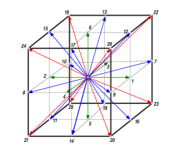
Figure 5: The 27 discrete velocity lattice in three spatial dimensions (D3Q27).

The local equilibria (a truncated version of Maxwell-Boltzmann distribution) encode the mass-momentum conservation laws. At the moment, they are purely classical, but the y can be easily extended to quantum statistics. In detail, [5]:

$$f_{i}^{A,eq}=w_{i}\rho_{A}(1+u_{i})$$ (33)

$$f_{i}^{B,eq}=w_{i}\rho_{B}(1+u_{i})$$ (34)

$$f_{i}^{C,eq}=w_{i}\rho_{C}(1+u_{i}+q_{i}/2)$$ (35)

where $u_{i}=\vec{u}\cdot\vec{c}_{i}/c_{s}^{2}$ and $q_{i}=u_{i}^{2}-u^{2}$, $u$ being the magnitude of the net flow of the carrier fluid, namely

$$\rho\vec{u}=\sum_{i}f_{i}^{C}\vec{c}_{i}$$ (37)

with

$$\rho=\sum_{i}f_{i}^{C}$$ (38)

the carrier density. Finally, $w_{i}$ is the standard set of weights normalised to unity and $c_{s}^{2}=\sum_{i}w_{i}c_{i}^{2}/d$ is the sound speed in $d$ spatial dimensions. In the present lattice $c_{s}^{2}=1/3$ (Note that the speed of light is $c=1$ in lattice units).

The transport properties are controlled by the relaxation rate, according to the standard LB relations, namely:

$$D_{A}=c_{s}^{2}(\tau_{A}-\Delta t/2),\;D_{B}=c_{s}^{2}(\tau_{B}-\Delta t/2),\;\nu_{C}=c_{s}^{2}(\tau_{C}-\Delta t/2)$$ (39)

Note that $A$ and $B$ equilibria conserve only mass, hence they support mass diffusion, whereas carrier $C$ equilibria conserve momentum as well because the local equilibria contain the self-consistent carrier current, see Eq. (37). Consequently the carrier relaxation rate controls momentum diffusivity, also known as kinematic viscosity.

For species $A$ and $B$, the forcing terms are set to zero $F_{i}^{A}=F_{i}^{B}=0$, so that they obey an ideal equation of state

$$p_{A,B}=\rho_{A,B}c_{s}^{2}.$$

Given that $c_{s}^{2}=1/3$ in lattice units, where $c=\Delta x/\Delta t=1$ is the light speed.

The carrier fluid, however, is subject to self-consistent force resulting from potential energy interactions, according to the standard LB pseudo-potential formulation [17]. Consequently, it obeys a non-ideal equation of state of the form (Carnahn-Starling) [3, 11]

$$\frac{p_{C}}{\rho_{C}v_{T}^{2}}=\frac{1+r+r^{2}+r^{3}}{(1-r)^{3}}-0.5r$$ (40)

where $v_{T}^{2}=k_{B}T/m$ and $r$ is the reduced carrier density. This corresponds to a critical temperature $T_{c}=0.047$ and density $\rho_{c}=0.066$ in lattice units.

10.1 Relaxation time as a function of the carrier density

,

In the present paper, we assume a discontinuous jump between the inner and outer space, although smoother dependencies could be easily adjusted. In the LB scheme, the diffusivity is controlled by the relaxation frequency $\omega\equiv 1/\tau$, hence the jump in diffusivity implies a corresponding change of such frequency across the membrane, Having stipulated $\omega_{out}=1$, the relation (39) implies: $2/\omega_{in}-1=D_{in}/D_{out}$, that is:

$$\tau_{out}=1,\;\;\;\tau_{in}=\frac{1}{2}(1+D_{in}/D_{out})$$

The diffusivity jump $J=D_{in}/D_{out}$ is then the only symmetry-breaking parameter to be varied in the simulations without sources. For the source-driven case we set, $F_{i}^{k}=W_{i}s^{k}$, see equation (1) in the text.

References

- [1] R. Benzi, S. Succi, and M. Vergassola. The lattice boltzmann equation: theory and applications. Physics Reports, 222(3):145 – 197, 1992.
- [2] Laurent Canetti, Marco Drewes, and Mikhail Shaposhnikov. Matter and antimatter in the universe. New Journal of Physics, 14(9):095012, sep 2012.
- [3] Norman F Carnahan and Kenneth E Starling. Equation of state for nonattracting rigid spheres. The Journal of Chemical Physics, 51(2):635–636, 1969.
- [4] Giacomo Falcucci, Giorgio Amati, Vesselin K Krastev, Andrea Montessori, Grigoriy S Yablonsky, and Sauro Succi. Heterogeneous catalysis in pulsed-flow reactors with nanoporous gold hollow spheres. Chemical Engineering Science, 166:274–282, 2017.
- [5] Giacomo Falcucci, Sauro Succi, Andrea Montessori, Simone Melchionna, Pietro Prestininzi, Cedric Barroo, David C Bell, Monika M Biener, Juergen Biener, Branko Zugic, et al. Mapping reactive flow patterns in monolithic nanoporous catalysts. Microfluidics and Nanofluidics, 20(7):105, 2016.
- [6] Willem Hundsdorfer and Jan G Verwer. Numerical solution of time-dependent advection-diffusion-reaction equations, volume 33. Springer Science & Business Media, 2013.
- [7] Leonard S Kisslinger. Astrophysics and the Evolution of the Universe. World Scientific Publishing Company, 2016.
- [8] Timm Krüger, Halim Kusumaatmaja, Alexandr Kuzmin, Orest Shardt, Goncalo Silva, and Erlend Magnus Viggen. The lattice boltzmann method. Springer International Publishing, 10:978–3, 2017.
- [9] Andrei D Linde. Phase transitions in gauge theories and cosmology. Reports on Progress in Physics, 42(3):389, 1979.
- [10] A. Montessori, M. Lauricella, and S. Succi. Mesoscale modelling of soft flowing crystals. Philosophical Transactions of the Royal Society A: Mathematical, Physical and Engineering Sciences, 377(2142):20180149, 2019.
- [11] A Montessori, P Prestininzi, M La Rocca, and S Succi. Entropic lattice pseudo-potentials for multiphase flow simulations at high weber and reynolds numbers. Physics of Fluids, 29(9):092103, 2017.
- [12] Andrea Montessori and Giacomo Falcucci. Lattice Boltzmann Modeling of Complex Flows for Engineering Applications. Morgan & Claypool Publishers, 2018.
- [13] Andrea Montessori, Marco Lauricella, Elad Stolovicki, David A. Weitz, and Sauro Succi. Jetting to dripping transition: Critical aspect ratio in step emulsifiers. Physics of Fluids, 31(2):021703, 2019.
- [14] David E Morrissey and Michael J Ramsey-Musolf. Electroweak baryogenesis. New Journal of Physics, 14(12):125003, 2012.
- [15] Antonio Riotto and Mark Trodden. Recent progress in baryogenesis. Annual Review of Nuclear and Particle Science, 49(1):35–75, 1999.
- [16] Andrei Dmitrievich Sakharov. Violation of cp invariance, c asymmetry, and baryon asymmetry of the universe. Physics-Uspekhi, 34(5):392–393, 1991.
- [17] Xiaowen Shan and Hudong Chen. Lattice boltzmann model for simulating flows with multiple phases and components. Physical Review E, 47(3):1815, 1993.
- [18] Sergio Solorzano, Miller Mendoza, Sauro Succi, and Hans Jürgen Herrmann. Lattice wigner equation. Physical Review E, 97(1):013308, 2018.
- [19] Sauro Succi. The Lattice Boltzmann Equation: For Complex States of Flowing Matter. Oxford University Press, 2018.
- [20] Doug Toussaint and Frank Wilczek. Particle–antiparticle annihilation in diffusive motion. The Journal of Chemical Physics, 78(5):2642–2647, 1983.
- [21] Douglas B Weibel and George M Whitesides. Applications of microfluidics in chemical biology. Current opinion in chemical biology, 10(6):584–591, 2006.