Spectral-Energy Efficiency Trade-off-based Beamforming Design for MISO Non-Orthogonal Multiple Access Systems

Abstract

Energy efficiency (EE) and spectral efficiency (SE) are two of the key performance metrics in future wireless networks, covering both design and operational requirements. For previous conventional resource allocation techniques, these two performance metrics have been considered in isolation, resulting in severe performance degradation in either of these metrics. Motivated by this problem, in this paper, we propose a novel beamforming design that jointly considers the trade-off between the two performance metrics in a multiple-input single-output non-orthogonal multiple access system. In particular, we formulate a joint SE-EE based design as a multi-objective optimization (MOO) problem to achieve a good trade-off between the two performance metrics. However, this MOO problem is not mathematically tractable and, thus, it is difficult to determine a feasible solution due to the conflicting objectives, where both need to be simultaneously optimized. To overcome this issue, we exploit a priori articulation scheme combined with the weighted sum approach. Using this, we reformulate the original MOO problem as a conventional single objective optimization (SOO) problem. In doing so, we develop an iterative algorithm to solve this non-convex SOO problem using the sequential convex approximation technique. Simulation results are provided to demonstrate the advantages and effectiveness of the proposed approach over the available beamforming designs.

I Introduction

Over recent years, extensive research efforts have been devoted to the practical implementations of new disruptive technologies for the fifth generation (5G) and beyond wireless networks [1]. The unexpected exponential growth in the number of connected devices and the unprecedented requirements of higher data rates, low latency and ultra reliability are of major concerns in future wireless networks [1]. However, these demanding requirements are difficult to meet or almost impossible to achieve without an enormous power consumption, which is not only unacceptable due to undesirable impacts on the natural environmental [2], but also financially unaffordable. Therefore, it is important to consider both as performance metrics, the spectral efficiency (SE) and energy efficiency (EE), simultaneously. SE is defined as the ratio between the achieved rate and the available bandwidth, whereas EE is defined as the ratio between the achieved sum rate in the system and the total required power to achieve this sum rate [3].

Different disruptive technologies, including massive multiple-input multiple-output (MIMO) [4] [5], millimeter-wave (mmWave) [1] [6] [7], and non-orthogonal multiple access (NOMA) techniques [8] have been proposed to meet the stringent design and operational requirements surrounding EE and SE. In particular, NOMA has been envisioned as one of the key techniques for significantly improving the SE while providing massive connectivity to support the Internet-of-Things (IoT) in 5G and beyond wireless networks [9]. Unlike the conventional orthogonal multiple access (OMA) schemes, the users in NOMA can be served within the same resource blocks such as time, frequency, and code without any orthogonal divisions between them, by exploiting the power-domain multiplexing [10]. For instance, superposition coding (SC) is utilized at the base station to encode the transmit signals of multiple users with different transmit power levels [11] [12]. At the receiver end, successive interference cancellation (SIC) is employed at the strong users (i.e., the users with stronger/better channel gains) to detect and remove the interference caused by signals intended to the weaker users prior to decoding their own desired signals [8].

To exploit different potential benefits, NOMA has been recently integrated with different technologies such as cognitive radio (CR) [13], millimeter-wave [14] [15], multiple-antenna techniques [16], [17], [18] and conventional OMA techniques [19]. In particular, the combination of NOMA with spatial domain multiple access (SDMA) offered by multiple-antenna can provide additional benefits, by jointly utilizing both the spatial and power domains. The notion of joint utilization of multiple domains helps meeting the demanding requirements in future wireless networks, particularly when compared against conventional stand alone SDMA techniques [16], [20]. For instance, incorporating NOMA with the multiple-antenna techniques was considered in [20]. Another example is multiple-input single-output (MISO)-NOMA  [21] [22] [23], which can be classified into two main categories: beamformer-based and cluster-based MISO-NOMA schemes [24] [25]. In this paper, we focus on the beamformer-based MISO-NOMA scheme, where each user is served by a single beamforming vector. For the sake of notational simplicity, the beamformer-based MISO-NOMA is referred to as MISO-NOMA throughout this paper.

One of the conventional beamforming designs developed for MISO-NOMA systems in the literature considers SE as a performance metric with the sum rate maximization (SRM) problem [26]. This SRM design is developed not only at the cost of the exponential increase in the available power, but also with significant loss in the EE performance. In fact, with the unprecedented growth in the number of mobile devices and volume of mobile data traffic in future wireless networks, EE becomes a prominent performance metric. This is primarily due to the fact that EE has the potential to achieve a good balance between the transmit power consumption and system throughput [3]. To overcome the EE degradation associated with the SRM design, we have proposed a global EE maximization (GEE-Max) design in our previous work [27] to maximize the overall EE of the system. However, a major drawback of such a design is that the base station does not have the flexibility to utilize the available power resources after achieving the maximum EE with its green power. In fact, this limitation becomes an important issue that needs to be addressed in some of the scenarios, such as base station being powered by renewable energy sources [27, 28]. Therefore, the trade-off between SE and EE motivates one to explore novel design approaches for beamforming so that a good balance between SE and EE performance metrics can be achieved. Furthermore, this joint SE-EE design provides flexibility to the base station to adapt the beamforming design by taking the instantaneous transmission conditions and the different requirements of the system into consideration. In particular, the practical applications of the proposed SE-EE trade-off design can be summarized as follows:

• Base stations with hybrid power sources are expected to play a crucial role on the deployments of 5G and beyond wireless networks [29]. These hybrid base stations are powered by either non-renewable energy sources such as diesel generators, or renewable energy sources such as photovoltaic panels and wind turbines to provide the communication services [30], alternately. For such hybrid base stations, the priority to choose either EE or SE depends on the available energy source, i.e., if the base station utilizes a renewable energy resource, then the importance of EE becomes less than that of SE, and vice-versa for non-renewable energy sources. Hence, an SE-EE trade-off based design offers flexibility to the base station to switch between different design criteria based on the available energy source.

• Furthermore, some resource allocation techniques aim to maximize EE with an SE constraint [31] [32]. However, this design limits the performance of either SE or EE due to its inflexibility [33]. Hence, the SE-EE trade-off based design has a potential capability to achieve a good balance between these conflicting performance metrics, especially in some practical applications where both SE and EE have similar importance.

The joint SE and EE-based design can be developed by formulating a multi-objective optimization (MOO) problem with these two performance metrics in the multi-objective function. In contrast to a unique global optimal solution in the conventional single objective optimization (SOO) problems, the MOO problems have many Pareto-optimal solutions which would yield a better performance in one of the multiple objectives [34], [35]. However, the required Pareto-optimal solution will be determined based on the relative importance of each objectives in the overall problem. Therefore, the decision maker (DM) (i.e., the base station in our scenario) has to firstly articulate the weights of each objective prior to evaluate the solution for the MOO problem, which is referred as a priori articulation in the literature [36]. Then, those multiple objectives are converted into a single objective function known as the utility function to represent the corresponding multi-objective functions [37]. In particular, many utility functions have been considered in the literature for different MOO problems, including the weighted-sum [35], the weighted-product, and the weighted max-min function [34]. As the MOO problems have different Pareto-optimal solutions, the DM chooses the best trade-off solutions (Pareto-optimal solutions) [34]. It is worth mentioning that the SE-EE trade-off designs have been considered in the wireless communications literature. For example, an SE-EE design for a point-to-point communication link is considered in [33]. Furthermore, a generalized framework for the SE-EE trade-off was investigated for orthogonal frequency-division multiplexing (OFDM) in [38]. Additionally, a multi-objective optimization approach is considered for link adaptation in an OFDM-based cognitive system in [39], where throughput and transmit power are simultaneously optimized. A number of MOO-based resource allocation techniques can be found in [31], [40]-[41].

I-A Contributions

Motivated by the importance of both key performance metrics SE and EE in 5G and beyond wireless networks [1], [42], and to overcome the limitations associated with the conventional GEE-Max and SRM designs [27]-[26], in this paper we propose an SE-EE trade-off based design for an MISO-NOMA system. Unlike the conventional designs, this SE-EE design optimizes SE and EE simultaneously to achieve a good balance between these conflicting performance metrics. In doing that, we make the following key contributions:

• We formulate the overall SE-EE design as a MOO problem. Although this renders the overall problem as a challenging form, where direct approaches for obtaining a feasible solution are inherently difficult, it offers an avenue for achieving a good balance between SE and EE. This approach is radically different from the conventional approaches, such as those outlined in [17, 26, 27], and [43]. More specifically, conventional optimization techniques, which are often employed in the context of the SOO problems, cannot directly be applied to solve this MOO problem. Our design approach provides a generic framework, where the GEE max and SE max designs can be considered as special cases by setting appropriate weight factors;

• We provide an algorithm to solve this non-trivial MOO problem. This algorithm utilizes a priori articulation method combined with weighted-sum utility function to recast the MOO problem into a form of an SOO problem [34]-[36];

• We prove that solving the SOO problem provides a Pareto-optimal solution to the original MOO problem. In particular, the sequential convex approximation (SCA) is exploited in the context of handling the non-convexity of the SOO problem.

The rest of the paper is organized as follows. In Section II, the system model and the problem formulation are introduced to represent the SE-EE trade-off-based design. Section III presents the proposed techniques to tackle the SE-EE trade-off-based design. To verify the proposed beamforming design, numerical results are provided in Section IV, where the performance of the proposed beamforming design is compared with that of the conventional beamforming design criteria. Finally, conclusions are drawn in Section V.

I-B Notations

We use lower case boldface letters for vectors and upper case boldface letters for matrices. $(\cdot)^{H}$ denotes complex conjugate transpose, and $\Re(\cdot)$ and $\Im(\cdot)$ stand for real and imaginary parts of a complex number, respectively. The symbols $\mathbb{C}^{N}$ and $\mathbb{R}^{N}$ denote $N$-dimensional complex and real spaces, respectively. $||\cdot||_{2}$ and $|\cdot|$ represent the Euclidean norm of a vector and the absolute value of a complex number, respectively. $\mathbf{x}\succ 0$ means that all the elements in the vector $\mathbf{x}$ are greater than zero.

II System Model And Problem Formulation

II-A System Model

We consider a downlink transmission of a MISO-NOMA system with $K$ single-antenna users in which a base station equipped with $N$ antennas simultaneously transmits to these $K$ users. The transmit signal from the base station is given by

$$\mathbf{x}=\sum_{j=1}^{K}\mathbf{w}_{j}s_{j},$$ (1)

where $s_{j}$ and $\mathbf{w}_{j}$ $\in$ $\mathbb{C}^{N\times 1}$ represent the symbol intended to the $j^{th}$ user, and the corresponding beamforming vector, respectively. It is assumed that these symbols (i.e., $s_{j},\forall j$) are independent and with unity power. In addition, digital beamforming is considered; hence, each user is served with a dedicated beamforming vector. As a result, we do not impose any constraint on the relationship between $K$ and $N$ and the proposed design is valid for any number of antennas and users. The received signal at the $i^{th}$ user can be written as

$$y_{i}=\sum_{j=1}^{K}\mathbf{h}_{i}^{H}\mathbf{w}_{j}s_{j}+n_{i},$$ (2)

where $n_{i}$ represents the zero-mean additive white Gaussian noise (AWGN) with variance $\sigma_{i}^{2}$, while $\mathbf{h}_{i}$ $\in$ $\mathbb{C}^{N\times 1}$ denotes the vector that contains the channel coefficients between the base station and the $i^{th}$ user. Furthermore, we assume frequency-flat channel conditions, and the channel coefficients can be modelled as

$$\mathbf{h}_{i}=\sqrt{d_{i}^{-\kappa}}\mathbf{g}_{i},$$

where $\kappa$ and $\mathbf{g}_{i}$ are the path loss exponent, and the small scale fading, respectively, whereas $d_{i}$ represents the distance between the $i^{th}$ user and the base station in meters. We consider that perfect channel state information (CSI) of the users is available at the base station.

In the downlink power-domain NOMA, the power levels are assigned to the users based on their channel strengths such that the allocated power levels are inversely proportional to the channel strengths of the users [9] [8]. Furthermore, the stronger users (i.e., users with higher channel strengths) perform SIC by firstly decoding the signals intended to the users with weaker channel conditions, and then subtracting the decoded signals prior of decoding their own signals [8] [44]. The weaker users detect their signals by treating the interference caused by the signals intended to the stronger users as noise [45]. Hence, user ordering plays a crucial role in power allocations, users’ SIC capability, and the overall performance of the the NOMA systems. However, the optimal ordering could be determined through performing an exhaustive search among all the user ordering possibilities, which is not practical to implement, especially in dense networks. Therefore, we consider the first user (U₁) as the strongest user in the cell, whereas the U_K is the weakest user based on the following channel conditions:

$$\underbrace{||\mathbf{h}_{K}||^{2}}_{\text{Weakest }}\leq||\mathbf{h}_{K-1}||^{2}\leq\cdots\leq\underbrace{||\mathbf{h}_{1}||^{2}}_{\text{Strongest}}.$$ (3)

Based on this user ordering, to ensure that the power allocated to each user in the system is inversely proportional to its channel gain, and to successfully implement SIC at the stronger users [26], the following conditions should be satisfied with the beamforming design [27]:

$$|\mathbf{h}_{i}^{H}\mathbf{w}_{K}|^{2}\geq\cdots\geq|\mathbf{h}_{i}^{H}\mathbf{w}_{1}|^{2},\forall i\in\mathcal{K}.$$ (4)

It is worthy to point out that some work in the context of downlink NOMA transmission literature assumes that NOMA transmission can be achieved without including the constraint in (4), such as in [46]. However, this power allocation constraint facilitates the design SIC orders, and has been assumed in most of the works in the literature to ensure successful implementation of SIC.

Therefore, the received signal at U_i after performing SIC is written as

$$\overset{*}{y_{i}}=\underbrace{\mathbf{h}_{i}^{H}\mathbf{w}_{i}s_{i}}_{\text{Intended signal }}+\underbrace{{\sum_{j=1}^{i-1}\mathbf{h}_{i}^{H}\mathbf{w}_{j}s_{j}}}_{\text{Interference }}+\underbrace{n_{i}}_{\text{Noise }},\forall i\in\mathcal{K},$$ (5)

where $\mathcal{K}\overset{\bigtriangleup}{=}\{1,\cdots,K\}$. Note that the interference caused by U${}_{i+1},\cdots,$U_K is removed through SIC. Furthermore, U_k has the capability to decode the message of U_i ($k\leq i$) with signal-to-interference and noise ratio (SINR) that can be written as

$$\text{SINR}^{(i)}_{k}=\frac{|\mathbf{h}_{k}^{H}\mathbf{w}_{i}|^{2}}{\sum_{j=1}^{i-1}|\mathbf{h}_{k}^{H}\mathbf{w}_{j}|^{2}+\sigma_{k}^{2}},\forall i\in\mathcal{K},k\leq i.$$ (6)

Now, with the assumption that $s_{i}$ is only decodable provided its SINR is higher than a threshold denoted as SINR^th, this explicitly requires that decoding of $s_{i}$ at other stronger users should be also higher than this threshold [26], i.e., SINR${}_{k}^{(i)}\geq$ SINR^th, $\forall k=1,2,\cdots,i$. Based on this argument, the definition of SINR_i should take into account the decoding of $s_{i}$ at the stronger users in order to align with the basic principle of NOMA, namely SIC. Based on this requirement, the achievable SINR can be defined as follows:

$$\text{SINR}_{i}=\text{min}({\text{SINR}^{(i)}_{1},\text{SINR}^{(i)}_{2},\cdots,\text{SINR}^{(i)}_{i}}),\forall i\in\mathcal{K}.$$ (7)

Based on the above discussion, the achieved rate at U_i can be defined as [26]

$$R_{i}=\text{min}({R^{(i)}_{1},R^{(i)}_{2},R^{(i)}_{3},\cdots,R^{(i)}_{i}}),\forall i\in\mathcal{K}.$$ (8)

Note that $R^{(i)}_{k}$ is the rate of decoding $s_{i}$ at U_k, and it is given as

$$R^{(i)}_{k}=B_{w}\log_{2}\Bigg{(}1+\frac{|\mathbf{h}_{k}^{H}\mathbf{w}_{i}|^{2}}{\sum_{j=1}^{i-1}|\mathbf{h}_{k}^{H}\mathbf{w}_{j}|^{2}+\sigma_{k}^{2}}\Bigg{)},\forall i\in\mathcal{K},$$ (9)

where $B_{w}$ is the available bandwidth, set to be one in this analysis.

The global energy efficiency (GEE) of the system is defined as the ratio between the achieved sum rate of the system and the total power required to achieve this rate (bits/Joules) [3], and is expressed as

$$\text{EE}=\text{GEE}=\frac{\sum_{i=1}^{K}R_{i}}{\frac{1}{\epsilon_{0}}P_{t}+P_{l}},$$ (10)

where $\epsilon_{0}$ denotes the power amplifiers efficiency at the base station. Furthermore, $P_{l}$ and $P_{t}$ represent the power losses at the base station and the transmit power, respectively. Note that $P_{t}$ should be less than the the available power budget at the base station ($P_{ava}$) which can be expressed as the following constraint:

$$P_{t}=\sum_{i=1}^{K}||\mathbf{w}_{i}||_{2}^{2}\leq P_{ava},$$ (11)

For the MISO-NOMA system considered in this paper, the GEE maximization (GEE-Max) design can be formulated into the following optimization problem [27]:

$${OP_{EE}}: \underset{\{\mathbf{w}_{i}\}_{i=1}^{K}}{\text{max}}$$ GEE (12a)

subject to $$\sum_{i=1}^{K}||\mathbf{w}_{i}||^{2}_{2}\leq P_{ava},$$ (12b)

$$R_{i}\geq R^{th}_{i},\forall i\in\mathcal{K},$$ (12c)

$$(\ref{channels}).$$ (12d)

The constraint in (12c) ensures that each user can achieve minimum predefined threshold rate ($R^{th}_{i}$) which is referred to as minimum rate constraint. Furthermore, the constraint in (12d) facilitates the successful implementation of SIC which is referred to as the SIC constraint throughout this paper. It is worth mentioning that the GEE-Max problem ${OP_{EE}}$ is solved in [27] using the SCA technique and the Dinkelbach’s algorithm. In particular, the maximum GEE is achieved with a certain available power which is known as the green power in the literature [47] [48]. Beyond this green power, both GEE and the achieved sum rate saturate [49].
Now, we formulate the SE maximization (SE-Max) problem for the MISO-NOMA system defined in this paper, as follows [26]:

$${OP_{SE}}: \underset{\{\mathbf{w}_{i}\}_{i=1}^{K}}{\text{max }}$$ SE (13a)

subject to $$\sum_{i=1}^{K}||\mathbf{w}_{i}||^{2}_{2}\leq P_{ava}$$ (13b)

$$(\ref{channels}),$$ (13c)

where $\text{SE}=\frac{\sum_{j=1}^{K}R_{j}}{B_{w}}.$ Note that the SE-Max problem is equivalent to the conventional SRM with the assumption of unit bandwidth, i.e., $B_{w}=1$. Hence, without loss of generality, SE-Max and SRM refer to the same problem throughout this paper. In particular, this SE-Max problem is solved for the MISO-NOMA system in [26]. Note that if the minimum rate constraint in (12c) is added to the original SE-Max $OP_{SE}$, then, the modified SE-Max problem will be referred as SE-Max (min-rate) in this paper. It is obvious that these conventional SE-Max and GEE-Max designs maximize either EE or SE individually, without jointly considering them to achieve a trade-off between these performance metrics. In the following subsection, we develop a joint SE-EE trade-off design.

II-B Problem Formulation

For notation simplicity, we represent SE and EE (i.e., GEE) by the functions $f_{1}\left(\{\mathbf{w}_{i}\}_{i=1}^{K}\right)$ and $f_{2}\left(\{\mathbf{w}_{i}\}_{i=1}^{K}\right)$, respectively. In particular, we aim to develop a beamforming design that can jointly maximize these performance metrics (i.e., max $f_{1}\left(\{\mathbf{w}_{i}\}_{i=1}^{K}\right)~{}\text{and}~{}f_{2}\left(\{\mathbf{w}_{i}\}_{i=1}^{K}\right)$ with the given set of constraints. Therefore, the beamforming vectors that can achieve a trade-off between the conflicting SE and EE metrics in the considered MISO-NOMA system can be formulated into the following MOO problem:

$${OP}: \underset{\{\mathbf{w}_{i}\}_{i=1}^{K}}{\text{max}} \mathbf{f}\left(\{\mathbf{w}_{i}\}_{i=1}^{K}\right)$$ (14a)

subject to $$\sum_{i=1}^{K}||\mathbf{w}_{i}||^{2}_{2}\leq P_{ava},$$ (14b)

$$R_{i}\geq R^{th}_{i},\forall i\in\mathcal{K},$$ (14c)

$$(\ref{channels}).$$ (14d)

Note that the objective vector $\mathbf{f}\left(\{\mathbf{w}_{i}\}_{i=1}^{K}\right)$ consists of the SE and GEE functions, such that $\mathbf{f}\left(\{\mathbf{w}_{i}\}_{i=1}^{K}\right)=\left[f_{1}\left(\{\mathbf{w}_{i}\}_{i=1}^{K}\right),f_{2}\left(\{\mathbf{w}_{i}\}_{i=1}^{K}\right)\right]$. It is obvious that there is no global optimal solution that maximizes these conflicting objectives in $OP$ [34]. However, the MOO problem $OP$ searches for all possible best trade-off solutions, which are known as the Pareto-optimal solutions in the literature [36].

Definition 1. [35] [36] A feasible solution ${\{\mathbf{w}_{i}^{*}\}_{i=1}^{K}}$ is defined as a Pareto-optimal solution if there exists no other feasible solution ${\{\mathbf{w}_{i}^{{}^{\prime}}\}_{i=1}^{K}}$ such that $\mathbf{f}\left(\{\mathbf{w}_{i}^{{}^{\prime}}\}_{i=1}^{K}\right)\succ\mathbf{f}\left(\{\mathbf{w}_{i}^{*}\}_{i=1}^{K}\right)$. The set of all Pareto-optimal solutions are collectively defined as the Pareto front in the literature [35].

Therefore, our aim is to find the set of the feasible solutions that satisfy the Pareto-optimality conditions for this MOO problem. However, due to the fact that the original $OP$ problem might be infeasible with certain $P_{ava}$, we carry out a feasibility check prior to solving it. The feasibility check and the proposed methodology to solve the problem $OP$ are provided in the next section.

III Proposed Methodology

First, we carry out a feasibility check prior to solving the optimization problem $OP$. For infeasible problems, we propose another beamforming design. The feasible $OP$ is solved by reformulating it as SOO problem using a priori articulation technique combined with the weighted-sum approach. Then, the SCA technique is exploited to tackle the non-convexity issue of the SOO problem. At the end of this section, we provide some discussions on the convergence and the performance evaluation of the proposed SCA algorithm to solve $OP$.

III-A Feasibility Check

Firstly, it is worthy to mention that the original optimization problem $OP$ turns out to be infeasible when the minimum rate requirements at each user cannot be met with the available power budget at the base station (i.e., $P_{ava}$). Therefore, it is important to investigate the feasibility of the original problem $OP$ prior to solving it. In particular, this feasibility check can be performed through evaluating the minimum transmit power, referred as $P^{*}$, that is required to satisfy the minimum rate and SIC constraints, in (14c) and (14d), respectively. This $P^{*}$ can be determined through solving the following power minimization problem:

$${OP_{P}:~{}P^{*}}= \underset{\{\mathbf{w}_{i}\}_{i=1}^{K}}{\text{min}} \!\!\!\!\!\!\!\!\!\!\!\!\sum_{i=1}^{K}||\mathbf{w}_{i}||^{2}_{2}$$ (15a)

subject to $$(\ref{rate_cco}),(\ref{ccha}).$$ (15b)

Note that the original problem $OP$ can only be solved provided that $P^{*}\leq P_{ava}$, and is infeasible when $P^{*}$ is higher than the available power at the base station (i.e., $P_{ava}$). To overcome this infeasibility, an alternative beamforming design can be considered to maximize the sum rate with available power budget, as in $OP_{SE}$ defined in (13). Without loss of generality, we assume that $OP$ is feasible (i.e., $P^{*}\leq P_{ava}$), and propose an effective approach to solve it in the following subsection.

III-B Proposed Methodology

As mentioned before, we first reformulate the original MOO problem $OP$ into a SOO form. Then, we employ the SCA technique to solve the SOO problem. More details are provided in the following discussions.

III-B1 Single Objective Transformation

First, we use a priori articulation scheme where the base station determines the relative importance of each objective function prior to determining the beamforming vectors based on the design requirements. In particular, the weight factor $\alpha_{i}$ is assigned to the $i^{th}$ objective function (i.e., $f_{i}(\{\mathbf{w}_{i}\}_{i=1}^{K}$) to reflect its relative importance on the overall design, such that $\sum_{i=1}^{2}\alpha_{i}=1$, $\alpha_{i}\in[0,1]$. Then, the vector containing the objective functions in the original MOO problem (i.e., $OP$) is replaced with a single objective function known as the utility function in the literature. Note that the utility function is a single-objective function that can alternatively represent the original multi-objective function based on the importance of each objective function [34]. There are several utility functions available in the literature [34] [35] [36]; we choose the weighted sum approach as it provides the Pareto-optimal solution to the original problem, as shown in Theorem 1. Based on the previous discussion, the SOO framework that represents the original MOO problem $OP$ can be formulated as follows:

$${\overset{\sim}{OP}}: \underset{\{\mathbf{w}_{i}\}_{i=1}^{K}}{\text{max}} f_{EE-SE}\left(\{\mathbf{w}_{i}\}_{i=1}^{K}\right)$$ (16a)

subject to $$\sum_{i=1}^{K}||\mathbf{w}_{i}||^{2}_{2}\leq P_{ava},$$ (16b)

$$R_{i}\geq R^{th}_{i},\forall i\in\mathcal{K},$$ (16c)

$$(\ref{channels}),$$ (16d)

where $f_{EE-SE}\left(\{\mathbf{w}_{i}\}_{i=1}^{K}\right)=\sum_{l=1}^{2}\alpha_{l}f_{l}^{Norm}\left(\{\mathbf{w}_{i}\}_{i=1}^{K}\right)$. Note that $f_{1}^{Norm}\left(\{\mathbf{w}_{i}\}_{i=1}^{K}\right)$ and $f_{2}^{Norm}\left(\{\mathbf{w}_{i}\}_{i=1}^{K}\right)$ represent the unit-less normalized version of $f_{1}\left(\{\mathbf{w}_{i}\}_{i=1}^{K}\right)$ and $f_{2}\left(\{\mathbf{w}_{i}\}_{i=1}^{K}\right)$, respectively, which can be defined as

$$f_{1}^{Norm}\left(\{\mathbf{w}_{i}\}_{i=1}^{K}\right)=\frac{{f_{1}\left(\{\mathbf{w}_{i}\}_{i=1}^{K}\right)}}{{f_{1}}^{*}},$$ (17a)

$$f_{2}^{Norm}\left(\{\mathbf{w}_{i}\}_{i=1}^{K}\right)=\frac{f_{2}\left(\{\mathbf{w}_{i}\}_{i=1}^{K}\right)}{f_{2}^{*}},$$ (17b)

where $f_{1}^{*}$ and $f_{2}^{*}$ are the maximum values of SE and GEE, respectively. In particular, $f_{1}^{*}$ and $f_{2}^{*}$ can be determined through solving $OP_{SE}$ and $OP_{EE}$, respectively. Note that the normalization of the objectives in (17) is an important step in the context of solving the original MOO problem $OP$ due to several reasons. Firstly, it is obvious that the performance metrics GEE and SE have different units. Therefore, an addition of such (un-normalized) functions is neither allowable nor defines any meaningful performance metric. Secondly, as these two functions have completely different ranges, combining them uisng a weighted-sum utility function will certainly degrade the achievable objective value of the function with lower range [34]. Therefore, to treat both objective functions in a fair manner, we employ a unitless normalization, by dividing each objective function with its corresponding optimal value. With such a normalization, we obtain a non-dimensional objective function with an upper bound of one. Note that different normalization (i.e., transformations) methods have been considered for MOO problems in the literature [33], [34], [36]. For notation simplicity, we use $\alpha_{2}=\alpha$ and $\alpha_{1}=1-\alpha$. To examine the Pareto-optimality of ${\overset{\sim}{OP}}$, we present the following theorem:

Theorem 1

The solutions of the weighted-sum SOO problem in ${\overset{\sim}{OP}}$ provide the Pareto-optimal solutions for the original MOO ${OP}$ problem.

Proof: Please refer to Appendix A. $\blacksquare$

It is obvious that ${\overset{\sim}{OP}}$ turns out to be SE-Max (min-rate) when $\alpha=0$. Furthermore, the problem becomes GEE-Max with $\alpha=1$. However, a good balance between the conflicting SE and EE can be achieved through choosing an appropriate $\alpha$ between 0 and 1. To this end, we have transformed the original MOO problem $OP$ into a form of a SOO problem ${\overset{\sim}{OP}}$. However, the optimization problem ${\overset{\sim}{OP}}$ cannot be directly solved due to the non-convexity nature of the objective function and the corresponding constraints. To circumvent this non-convexity issue, we propose an effective approach to solve ${\overset{\sim}{OP}}$ in the next subsection.

III-B2 Sequential Convex Approximation

The SCA technique is an iterative approach to solve the original non-convex optimization problem by approximating the non-convex functions by lower-bounded convex functions [50] [51]. In particular, the SCA technique has been employed to solve different non-convex resource allocation problems in the literature [26] [27]. Similarly, we exploit the SCA technique to solve the ${\overset{\sim}{OP}}$ problem by approximating each non-convex term with a convex one. We start with the objective function by introducing two new slack variables $\Gamma_{1}$ and $\Gamma_{2}$ such that

$$(1-\alpha)f_{1}^{Norm}\left(\{\mathbf{w}_{i}\}_{i=1}^{K}\right)\geq\Gamma_{1},$$ (18a)

$$\alpha f_{2}^{Norm}\left(\{\mathbf{w}_{i}\}_{i=1}^{K}\right)\geq\Gamma_{2}.$$ (18b)

Based on these slack variables, the original ${\overset{\sim}{OP}}$ problem can be equivalently written as

$${\overset{\approx}{OP}}:\underset{\Gamma_{1},\Gamma_{2},\{\mathbf{w}_{i}\}_{i=1}^{K}}{\text{max}} \Gamma_{1}+\Gamma_{2}$$ (19a)

subject to $$\sum_{i=1}^{K}||\mathbf{w}_{i}||^{2}_{2}\leq P_{ava},$$ (19b)

$$R_{i}\geq R_{th},\forall i\in\mathcal{K},$$ (19c)

$$(\ref{channels}),$$ (19d)

$$\alpha f_{2}^{Norm}\left(\{\mathbf{w}_{i}\}_{i=1}^{K}\right)\geq\Gamma_{2},$$ (19e)

$$(1-\alpha)f_{1}^{Norm}\left(\{\mathbf{w}_{i}\}_{i=1}^{K}\right)\geq\Gamma_{1}.$$ (19f)

It is obvious that the objective function in $\overset{\approx}{OP}$ is a linear function in terms of $\Gamma_{1}$ and $\Gamma_{2}$. Furthermore, the constraints are not convex and we handle these non-convexity issues as follows. First, we look into the non-convexity of the constraint in (19f) by rewriting it as

$$\sum_{i=1}^{K}\log_{2}(1+\text{SINR}_{i})\geq\frac{f_{1}^{*}}{(1-\alpha)}\Gamma_{1}.$$ (20)

We handle this non-convexity issue by introducing new slack variables $z_{i},\rho_{i}$, such that

$$\log_{2}(1+\text{SINR}^{(i)}_{k})\geq\rho_{i},\forall i\in\mathcal{K},k\leq i,$$ (21a)

$$1+\text{SINR}^{(i)}_{k}\geq z_{i},\forall i\in\mathcal{K},k\leq i.$$ (21b)

Based on these multiple slack variables, the constraint in (20) can be equivalently written as the following set of constraints:

$$(\ref{ccc})\Leftrightarrow \sum_{i=1}^{K}\rho_{i}\geq\frac{f_{1}^{*}}{(1-\alpha)}\Gamma_{1},$$ (22a)

$$(\ref{ccc})\Leftrightarrow z_{i}\geq 2^{\rho_{i}},\quad\forall i\in\mathcal{K},$$ (22b)

$$(\ref{ccc})\Leftrightarrow (\ref{kok}).$$ (22c)

It is obvious that the inequalities (22a) and (22b) are convex constraints, whereas the constraint in (22c) remains still non-convex. Furthermore, we introduce another slack variable $a_{i,k}$ to convert it into a convex one as follows:

$${|\mathbf{h}_{k}^{H}\mathbf{w}_{i}|^{2}}\geq{(z_{i}-1)a_{i,k}^{2}},\forall i\in\mathcal{K},k\leq i,$$ (23a)

$$a_{i,k}^{2}\geq{\sum_{j=1}^{i-1}|\mathbf{h}_{k}^{H}\mathbf{w}_{j}|^{2}+\sigma_{k}^{2}},\forall i\in\mathcal{K},k\leq i.$$ (23b)

We handle the non-convexity issues in the constraint (23a) by approximating $|\mathbf{h}_{k}^{H}\mathbf{w}_{i}|^{2}$ with a lower bound which is chosen to be $\Re({\mathbf{h}_{k}^{H}\mathbf{w}_{i}})$, such that

$$|\mathbf{h}_{k}^{H}\mathbf{w}_{i}|^{2}\geq{\left(\Re({\mathbf{h}_{k}^{H}\mathbf{w}_{i}})\right)}^{2},\forall k,\forall i.$$ (24)

Note that the constraint in (24) is always held true for any set of channel coefficients and beamforming vectors, and thus, is not required to be included in the optimization problem. Now, we take the square-root of both sides in (23a) after incorporating the new approximation in (24). Next, the right-hand side of this inequality can now be approximated with linear function using the first-order Taylor series approximation. Based on that, the constraint in (23a) can be written in the following approximated convex form:

$$\Re({\mathbf{h}_{k}^{H}\mathbf{w}_{i}})\geq\sqrt{(z_{i}^{(n)}-1)}a_{i,k}^{(n)}\\ +0.5\frac{1}{\sqrt{(z_{i}^{(n)}-1)}}a_{i,k}^{(n)}(z_{i}-z_{i}^{(n)})\\ +\sqrt{(z_{i}^{(n)}-1)}(a_{i,k}-a_{i,k}^{(n)}),\forall i\in\mathcal{K},k\leq i,$$ (25)

where $a_{i,k}^{(n)}$ and $z_{i}^{(n)}$ represent the approximations of $a_{i,k}$ and $z_{i}$ in the n^th iteration, respectively. However, the constraint in (23b) can be reformulated into the following second-order cone (SOC) [52]:

$$a_{i,k}\geq||\left[\mathbf{h}_{k}^{H}\mathbf{w}_{i-1}\cdots\mathbf{h}_{k}^{H}\mathbf{w}_{1}~{}\sigma_{k}\right]^{T}||_{2},\forall i\in\mathcal{K},k\leq i.$$ (26)

Next, the non-convexity of the constraint in (19e) is tackled by introducing a new slack variable $b$ such that

$$\frac{\sum_{j=1}^{K}R_{j}}{\frac{1}{\in}P_{t}+P_{l}}\geq\frac{f_{2}^{*}}{\alpha}\frac{\Gamma_{2}b^{2}}{b^{2}},$$ (27)

hence, the constraint in (19e) can be split into the following two constraints:

$$\sum_{j=1}^{K}R_{j}\geq\frac{f_{2}^{*}}{\alpha}{\Gamma_{2}b^{2}},$$ (28a)

$${b^{2}}\geq{\frac{1}{\epsilon_{0}}\sum_{i=1}^{K}||\mathbf{w}_{i}||_{2}^{2}+P_{l}}.$$ (28b)

To resolve the non-convexity issue in (28a), we exploit the same approaches used to handle the constraint in (20) by introducing a set of new slack variables, $r_{i},\xi_{i,k}$, and $\rho_{i}$, such that

$$R_{i}\geq\rho_{i},\forall i\in\mathcal{K},$$ (29a)

$$\frac{|\mathbf{h}_{k}^{H}\mathbf{w}_{i}|^{2}}{\sum_{j=1}^{i-1}|\mathbf{h}_{k}^{H}\mathbf{w}_{j}|^{2}+\sigma_{k}^{2}}\geq(r_{i}-1)\frac{\xi_{i,k}^{2}}{\xi_{i,k}^{2}},\forall i\in\mathcal{K},k\leq i.$$ (29b)

Based on these multiple slack variables, the constraint in (28a) can be approximated through the following convex constraints:

$$\Re({\mathbf{h}_{k}^{H}\mathbf{w}_{i}})\geq\sqrt{(r_{i}^{(n)}-1)}\xi_{i,k}^{(n)}\\ +0.5\frac{1}{\sqrt{(r_{i}^{(n)}-1)}}\xi_{i,k}^{(n)}(r_{i}-r_{i}^{(n)})\\ +\sqrt{(r_{i}^{(n)}-1)}(\xi_{i,k}-\xi_{i,k}^{(n)}),\forall i\in\mathcal{K},k\leq i,$$ (30)

$$\xi_{i,k}\geq||\left[\mathbf{h}_{k}^{H}\mathbf{w}_{1}\cdots\mathbf{h}_{k}^{H}\mathbf{w}_{i-1}~{}\sigma_{k}\right]^{T}||_{2},\forall i\in\mathcal{K},k\leq i,$$ (31)

$$r_{i}\geq 2^{\rho_{i}},\quad\forall i\in\mathcal{K},$$ (32)

$$\sum_{j=1}^{K}{\rho_{i}}\geq\\ \frac{f_{2}^{*}}{\alpha}\Big{(}\Gamma_{2}^{(n)}{b^{2}}^{(n)}+2b^{(n)}\Gamma_{2}^{n}(b-b^{(n)})+{b^{2}}^{(n)}(\Gamma_{2}-\Gamma_{2}^{(n)})\Big{)}.$$ (33)

Similar to the constraint in (23b), the constraint in (28b) can be cast as the following SOC constraint:

$$b\geq\frac{1}{\sqrt{\epsilon_{0}}}||\left[||\mathbf{w}_{1}||_{2}~{}||\mathbf{w}_{2}||_{2}\cdots||\mathbf{w}_{K}||_{2}~{}\sqrt{P_{l}}\right]^{T}||_{2}.$$ (34)

To this end, the non-convex constraint in (19e) is replaced with the following convex constraints:

$$\text{(\ref{go})}\Leftrightarrow (\ref{slk}),(\ref{cuma1}),(\ref{s1c}),$$ (35a)

$$\text{(\ref{go})}\Leftrightarrow (\ref{lara1}),(\ref{haith}).$$ (35b)

Next, the non-convexity of the constraint in (19d) is handled by replacing each term in the inequality by a linear term using the first-order Taylor series expansion, such that

$$|\mathbf{h}_{k}^{H}\mathbf{w}_{i}|^{2}\geq||\left[\Re{\left(\mathbf{h}_{k}^{H}\mathbf{w}_{i}^{(n)}\right)}~{}\Im{(\mathbf{h}_{k}^{H}\mathbf{w}_{i}^{(n)})}\right]^{T}||^{2}\\ +2\left[\Re{(\mathbf{h}_{k}^{H}\mathbf{w}_{i}^{(n)})}~{}\Im{(\mathbf{h}_{k}^{H}\mathbf{w}_{i}^{(n)})}\right]\\ \big{[}(\Re{(\mathbf{h}_{k}^{H}\mathbf{w}_{i})}-\Re{(\mathbf{h}_{k}^{H}\mathbf{w}_{i}^{(n)})})(\Im{(\mathbf{h}_{k}^{H}\mathbf{w}_{i})}-\Im{(\mathbf{h}_{k}^{H}\mathbf{w}_{i}^{(n)})})\big{]}^{T}.$$ (36)

Note that the right-hand side of the inequality in (36) is linear in terms of $\mathbf{w}_{i}$. Hence, each term in the constraint in (19d) is replaced by the right-side of (36). Finally, we consider the constraint in (19c) with the following equivalent SINR constraint:

$$\frac{|\mathbf{h}_{k}^{H}\mathbf{w}_{i}|^{2}}{\sum_{j=1}^{i-1}|\mathbf{h}_{k}^{H}\mathbf{w}_{j}|^{2}+\sigma_{k}^{2}}\geq\eta^{th}_{i},\forall i\in\mathcal{K},k\leq i,$$ (37)

where $\eta^{th}_{i}=2^{R^{th}_{i}}-1$. Furthermore, the constraint in (37) can be reformulated as the following SOC constraint:

$$\frac{1}{\sqrt{\eta^{th}_{i}}}\Re({\mathbf{h}_{k}^{H}\mathbf{w}_{i}})\geq||\left[\mathbf{h}_{k}^{H}\mathbf{w}_{1}~{}\cdots\mathbf{h}_{k}^{H}\mathbf{w}_{i-1}~{}\sigma_{k}\right]^{T}||_{2},\\ \forall i\in\mathcal{K},k\leq i.$$ (38)

Based on these approximations, the original non-convex optimization problem ${\overset{\sim}{OP}}$ can be reformulated as

$${\overset{\cong}{OP}}:\underset{\Psi}{\text{Maximize }} \Gamma_{1}+\Gamma_{2}$$ (39a)

subject to $$(\ref{bn2}),(\ref{sec}),(\ref{s1c}),$$ (39b)

$$(\ref{cuma4}),(\ref{cuma5}),(\ref{slk}),(\ref{cuma1}),(\ref{const12}),$$ (39c)

$$(\ref{power}),(\ref{fst}),(\ref{lara1}),(\ref{haith}),$$ (39d)

where $\Psi$ consists of all the variables involved in this design, which can be expressed as
$\Psi=\{\mathbf{w}_{i},r_{i},b,\Gamma_{1},\Gamma_{2},z_{i},\xi_{i,k},a_{i,k},\rho_{i}\}_{i=1}^{K}.$

Note that the relationship between SE and EE basically shows two different trends with the available power. In the first trend, both SE and EE increase with the available power and this trend continues until the available power reaches the green power. Once the available power exceeds the green power, both SE and EE show the conflicting nature with the available power, which leads to the second trend. In order to shed more light on these trends, we provide the following lemma:

Lemma 1

The SE-EE optimization problem ${\overset{\sim}{OP}}$ provides the same solution with different weight factors $\{\alpha_{l}\}_{l=1}^{2}$ when the available power $P_{ava}$ is less than the green power (i.e., $P_{ava}\leq\text{ green power})$.

Proof: Please refer to Appendix B. $\blacksquare$
It is worth mentioning that the solution of ${\overset{\cong}{OP}}$ requires an appropriate selection of the initial parameters (i.e., $\Psi^{(0)}$). As this is an iterative approach, it is important to provide discussion on the initial conditions and the convergence of the proposed algorithm, which are presented in the following subsection.

III-C Initial Conditions, Convergence Analysis, Performance Evaluation, and Complexity Analysis

III-C1 Initial Conditions

Firstly, it is crucial to choose an appropriate set $\Psi^{(0)}$ to ensure the feasibility of the problem in the first iteration of the algorithm [19]. In particular, we choose a set of feasible beamforming vectors which can satisfy all the constraints in the approximated problem ${\overset{\cong}{OP}}$. Then, we determine all required slack variables in ${\overset{\cong}{OP}}$ based on chosen initial beamforming vectors. The proposed algorithm to solve the original $OP$ is summarized in Algorithm 1.

Algorithm 1: SE-EE trade-off maximization using SCA

Step 1: Check the feasibility of the problem

Step 2: Initialization of $\Psi^{(0)}$

Step 3: Repeat

1. Solve the optimization problem in (39)

2. Update $\Psi^{(n+1)}$

Step 4: Until required accuracy is achieved.

III-C2 Convergence Analysis

By making use of the analysis presented in [50], we provide the convergence analysis for the proposed algorithm. Let us first indicate that the optimization parameters at the n^th iteration (i.e., $\Psi^{(n)})$ are updated based on the solution obtained by solving the approximated optimization problem in (39). To ensure the convergence of this algorithm, three key conditions have to be satisfied. Firstly, appropriate initial conditions are chosen to ensure the feasibility of the approximated problem ${\overset{\cong}{OP}}$ at the first iteration of Algorithm 1. This provides a feasible solution to update the parameters in the next iteration. It is worth mentioning that the feasible solution to the approximated problem can always ensure the original constraint. In order to provide an additional insight into this feasibility issue, we include the following lemma:

Lemma 2

Suppose that the feasible solution set of the optimization problem ${OP}$ is denoted by $\chi$; then, the feasible region of the approximated convex optimization problem $\Psi^{n}$ falls within the same feasible region of the original non-convex problem, i.e., $\Psi^{n}\subseteq\chi,\forall n$.

Proof: To prove this lemma, we firstly point out that the approximated optimization problem $\overset{\cong}{OP}$ is solved iteratively. As such, at each iteration, the solution of $\overset{\approx}{OP}$ is provided for the given set of convex constraints in (39). Using the first-order Taylor series expansion, these constraints in the original problem ${OP}$ are approximated with their lower bounds. This implies that the solution also lies within the same feasible region $\Psi^{n}$ and satisfies all the constraints in the original problem [50], i.e., $\Psi^{n}\subseteq\chi$, which completes the proof of Lemma 2. $\blacksquare$
Secondly, we present a new lemma to support that the objective function in ${\overset{\cong}{OP}}$ is non-decreasing with each iteration.

Lemma 3

The objective function in $\overset{\cong}{OP}$ is non-decreasing in terms of $\Psi^{n}$, i.e., $\Upsilon(\Psi^{(n+1)})\geq\Upsilon(\Psi^{(n)})$, where $\Upsilon(\Psi^{(n)})=\Gamma_{1}(\Psi^{(n)})+\Gamma_{2}(\Psi^{(n)})$.

Proof: To prove this lemma, we point out that the solution of ${\overset{\cong}{OP}}$ at the $n^{th}$ iteration is a feasible solution to ${\overset{\cong}{OP}}$ in the next iteration. This inherently means that the objective function value at the $n^{th}$ iteration, ${\Upsilon(\Psi^{(n)}})$, is less than or equal to that obtained in the subsequent iteration, ${\Upsilon(\Psi^{(n+1)}})$, which means that ${\Upsilon(\Psi)}$ is non-decreasing function [50]. This completes the proof of Lemma 3. $\blacksquare$
Therefore, the objective value at each iteration will either increase or remain the same. Finally, the power constraint in (14b) ensures that the objective function of ${\overset{\cong}{OP}}$ is upper bounded due to the fact that $P_{ava}<<\infty$. In particular, the satisfaction of these three conditions ensures that the developed SCA technique converges to a solution with a finite number of iterations.

III-C3 Performance Evaluation

The solution of ${\overset{\sim}{OP}}$ is obtained by introducing multiple slack variables and iteratively solving the problem with different approximations. Hence, the performance evaluation of the proposed approach is important to assess its effectiveness. As such, we compare the performance of the proposed Algorithm 1 with a benchmark scheme. In particular, we use the power minimization problem $OP_{P}$ as a benchmark scheme by reformulating it as a semi-definite programming (SDP) which provides the optimal solution [53] [54]. In this SDP, we set the rates that are achieved through solving ${\overset{\sim}{OP}}$ as the minimum rate requirements for $OP_{P}$ and those achieved rates are denoted by $R_{i}^{*}$, $\forall i\in\mathcal{K}$. Then, we set these rates as minimum rate targets for $OP_{P}$. Without loss of generality, with introducing new rank-one matrices $\mathbf{W}_{i}=\mathbf{w}_{i}^{H}\mathbf{w}_{i}$ and exploiting semi-definite relaxation, the SDP form of $OP_{P}$ can be formulated with minimum rate constraints as follows [55]:

$${\overset{\sim}{OP_{P}}}:\underset{\{\mathbf{W}_{i}\}_{i=1}^{K}}{\text{minimize }} \sum_{i=1}^{K}\text{Tr}[\mathbf{W}_{i}]$$ (40a)

subject to $$\text{Tr}[\textbf{H}_{k}\mathbf{W}_{i}]-\eta_{i}^{*}\sum_{j=1}^{i-1}\text{Tr}[\textbf{H}_{k}\mathbf{W}_{j}]\geq$$

$$\eta_{i}^{*}\sigma_{k}^{2},\forall i\in\mathcal{K},k\leq i,$$ (40b)

$$\text{Tr}[\textbf{H}_{i}\mathbf{W}_{1}]\leq\text{Tr}[\textbf{H}_{i}\mathbf{W}_{2}]\leq\cdots$$

$$\leq\text{Tr}[\textbf{H}_{i}\mathbf{W}_{K}],\forall i\in\mathcal{K},$$ (40c)

$$\mathbf{W}_{i}=\mathbf{W}_{i}^{H},\mathbf{W}_{i}\succeq 0,\forall i\in\mathcal{K},$$ (40d)

where $\eta_{i}^{*}=2^{R_{i}^{*}}-1$, while $\textbf{H}_{i}=\mathbf{h}_{i}\mathbf{h}_{i}^{H}$. The solutions (i.e., the beamforming vectors) achieved through solving ${\overset{\sim}{OP_{P}}}$ are optimal and will also be the solutions to the original problem $OP_{P}$ provided that they are rank-one matrices [43], [53]. Note that the beamforming vectors are determined through extracting the eigenvectors corresponding to the maximum eigenvalues of these rank-one matrices [56]. In particular, we demonstrate in the simulation results that the proposed SCA technique to solve ${\overset{\sim}{OP}}$ provides approximately similar performance of ${\overset{\sim}{OP_{P}}}$.

III-C4 Complexity Analysis of the Proposed SCA Technique

Considering the fact that an iterative SCA algorithm is adopted to solve the original problem $OP$, it is crucial to define the computational complexity of the proposed algorithm. This can be achieved through determining the complexity associated with solving the approximated convex optimization problem $\overset{\cong}{OP}$ at each iteration of this algorithm. In particular, at each iteration, a linear objective function (i.e., $\Gamma_{1}+\Gamma_{2}$) is optimized with a set of SOC and linear constraints, where the interior-point method is employed to obtain the solution at each iteration [57], [58]. Therefore, the computational complexity at each iteration is primarily defined considering the complexity of obtaining the solution of such second-order cone programme (SOCP). In general, the work required to solve an SOCP problem is at most $\mathcal{O}(\mathcal{B}^{2}\mathcal{V})$ [58], where $\mathcal{B}$ and $\mathcal{V}$ denote the number of optimization variables and the total dimensions of the SOCP optimization problem, respectively. Furthermore, an iterative algorithm converges to a solution with an upper bound given as $\mathcal{O}(\sqrt{\mathcal{C}}\log(\frac{1}{\epsilon}))$, where $\mathcal{C}$ and $\epsilon$ are the total number of constraints at each iteration and the required accuracy, respectively. Now, with the developed SCA in hand, $\mathcal{B}$ and $\mathcal{V}$ are estimated as $(1.5{K^{2}}+4.5K+2NK+3+c)$ and $(5.5{K^{2}}+5K+2NK+4+c)$, respectively, where $c$ is a constant related to the number of constraints that arise due to the relaxation of the exponential constraints in the interior-point method [59]. Furthermore, the total number of constraints $\mathcal{C}$ in $\overset{\cong}{OP}$ is found to be $(2.5K^{2}+6.5K+6+c)$.

IV Simulation Results

In this section, we provide simulation results to support the effectiveness of the proposed SE-EE trade-off beamforming design of a downlink MISO-NOMA system over the conventional designs. In particular, we study the impact of the trade-off between the achieved EE and SE. In these simulations, we consider a base station equipped with three transmit antennas (i.e., $N=3$), which simultaneously transmits to five single-antenna users that are located at a distance of 1, 2, 3, 4, and 50 meters from the base station, respectively. The small-scale fading is chosen to be Rayleigh fading, while the path loss exponent $\kappa$ and the noise variance of all users $\sigma^{2}$ are both set to be 1. In addition, the minimum SINR thresholds are set to be $10^{-2}$ for all the users, i.e., $\eta_{th}=10^{-2}$. The amplifiers’ gain $\epsilon_{0}$ is set to $0.65$, whereas the power losses at the base station are assumed to be $40$ dBm (i.e., $P_{l}=40$ dBm). Furthermore, we define the available power at the base station by TX-SNR in dB, such that $\text{TX-SNR (dB)}=10\log_{10}\frac{P_{ava}}{\sigma^{2}}.$ In addition, the available bandwidth of transmission is assumed to be 1 MHz, i.e., $B_{w}=1$ MHz. Furthermore, the algorithm terminates when the difference between two consequent outputs is less than 0.001 (i.e., $\varepsilon\leq 0.01$). Finally, we define the achieved sum rate of the cell as

$$\text{sum rate}=B_{w}\text{SE}.$$

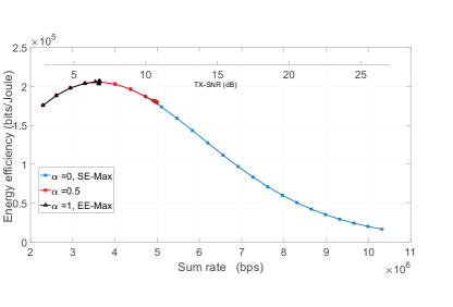
Figure 1: Achieved EE and sum rate against TX-SNR with different weight factors $\alpha$.

Fig. 1 illustrates the achieved EE and sum rate versus different TX-SNR and for different weight factors $\alpha$. As seen in Fig. 1, the SE-EE trade-off design considered in ${\overset{\sim}{OP}}$ turns out to be SE-Max with $\alpha=0$. Furthermore, ${\overset{\sim}{OP}}$ keeps maximizing the sum rate as TX-SNR increases at the cost of EE degradation. This is due to the fact that the GEE (i.e., EE) has been assigned with zero weight (i.e., $\alpha=0$) in the MOO problem. However, with $\alpha=1$, the problem is transformed into a GEE-Max design; as a result, the maximum EE is achieved with certain power threshold, referred as green power in the literature. Beyond this green power, no further enhancement is achieved either in the EE or in the sum rate. Furthermore, this design has the flexibility to strike a good balance between EE and the sum rate by setting the weight factor $\alpha$ between 0 and 1. For example, when $\alpha=0.5$, an increment in the sum rate is attained compared to that obtained with $\alpha=1$, as seen in Fig. 1. However, this sum rate enhancement is attained at the cost of EE degradation.

Fig. 2 presents the achieved EE and sum rate with different weight factors for 5 and 25 dB TX-SNR thresholds. In particular, Fig. 2 shows two different behaviors. First, both performance metrics (i.e., sum rate and EE) remain constant with the available power lower than the green power for different weight factors $\alpha$, which supports the validation of Lemma 1. However, as TX-SNR exceeds the green power, for example with TX-SNR= 25 dB, the trade-off between EE and sum rate can be realized by varying the weight factor. In particular, at this TX-SNR threshold, the achieved rate and EE show a performance in the range of 10-3.5 Mbps and 0.02-0.2 Mbits/Joule, respectively. This performance range is achieved with different weight factors $\alpha$, as presented in Fig. 2. Note that the base station in the proposed SE-EE trade-off design offers a wide-range of SE-EE trade-off through a possibility of simply tuning the weigh factor $\alpha$. In fact, this flexibility is beneficial for different practical applications where the transmission techniques can be adaptive according to the available power resources.

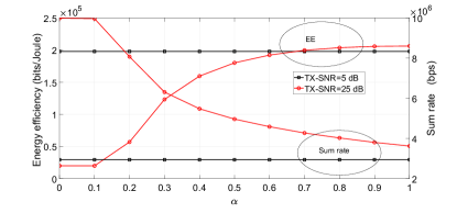
Figure 2: Achieved EE and sum rate with different weight factors $\alpha$.

(a)

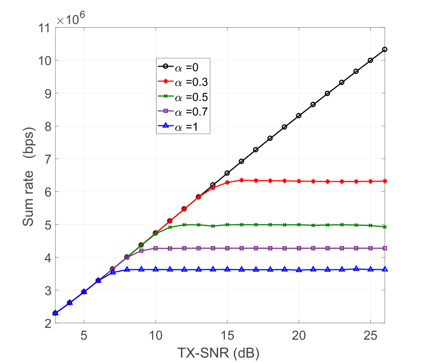
(b)

Figure 3: The EE and sum-rate performance of the proposed design versus TX-SNR, with different weight factors. (a) The achieved EE, (b) the achieved sum rate.

Furthermore, Figs. 3(a) and 3(b) show the achieved EE and sum rate versus TX-SNR for different weight factors $\alpha$, respectively. It can be clearly understood the impacts of the weight factors on the achieved EE and sum rate of the system. For example, at TX-SNR = 20 dB, EE declines from $2.2\times 10^{5}$ bits/Joule to $0.5\times 10^{5}$ bits/Joule by changing the weight factor from $\alpha=1$ to $\alpha=0$. However, the sum rate (i.e., SE) shows a different behavior. With TX-SNR = 20 dB, this decreases from $8.2\times 10^{6}$ bps to $3.6\times 10^{6}$ bps by changing the weight factor $\alpha$ from 0 to 1. Therefore, the proposed EE-SE trade-off design offers the flexibility to the base station to choose an appropriate weight factor based on the favorable conditions and system requirements to determine the desired performance metric.

TABLE I: Achieved EE and sum rate for the proposed design versus different TX-SNR, with different weight factors $\alpha$, $\eta_{th}=1$.

TX-SNR= 5 dB TX-SNR= 25 dB sum rate (Mbps) EE (Mbits/Joule) P (W) sum rate (Mbps) EE (Mbits/Joule) P (W) $\alpha=0$ 2.5301 0.1702 3.1623 9.3011 0.0187 316.2278 $\alpha=0.5$ 2.5301 0.1702 3.1623 6.4685 0.0635 59.7636 $\alpha=1$ 2.5301 0.1702 3.1623 5.5084 0.0685 45.7811

Furthermore, Fig. 4 demonstrates the impact of the minimum SINR threshold $\eta_{th}$ on the performance of the proposed design. In particular, with $\eta_{th}=2$, the original optimization problem becomes infeasible as the minimum required transmit power $P^{*}$ to achieve these minimum SINR requirements exceeds the available power $P_{ava}$. Hence, an alternative design, namely the SE-Max is considered. As a result, the achieved sum rate is maximized under the available power constraint which provides constant sum rate and EE over the different weight factors $\alpha$. However, choosing lower value of $\eta_{th}$ ensures the feasibility of the design, which can be observed with $\eta_{th}=0.2$, in Fig. 4. These results indicate that the base station has the flexibility to choose either EE or SE performance metric based on the available energy resource by selecting an appropriate weight factor $\alpha$. Furthermore, the joint SE-EE design problem boils down to an SRM and GEE-max problem with $\alpha=0$ and $\alpha=1$, respectively.

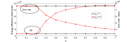
Figure 4: Achieved EE and sum rate for the proposed design versus weight factors $\alpha$, with different SINR thresholds $\eta_{th}$, TX-SNR= 20 dB.

In Table II, we show the performance of the proposed SCA algorithm. The rates achieved by solving $\tilde{OP}$ (i.e., $R_{i}^{*}$) are set as target SINR (i.e., $\eta_{i}^{*}$) for $\tilde{OP_{P}}$, where $\eta_{i}^{*}=2^{R_{i}^{*}}-1$. Then, the baseline optimization problem $\tilde{OP_{P}}$ is solved using the SDR approach. In fact, through analysing the information in Table II, we can confirm that the proposed SCA technique achieves approximately similar solution to that of the benchmark, $OP_{P}$.

TABLE II: Performance comparison between the proposed SCA algorithm to solve $\tilde{OP}$ and the benchmark solution obtained by solving $OP_{P}$ with $\eta_{th}=0.2$ and TX-SNR= 20 dB.

$\tilde{OP}$ $\tilde{OP_{P}}$ $R_{1}^{*}$ (Mbps) $R_{2}^{*}$ (Mbps) $R_{3}^{*}$ (Mbps) $R_{4}^{*}$ (Mbps) $R_{5}^{*}$ (Mbps) $R^{*}$ (Mbps) $P_{t}$ (W) $P^{*}$ (W) $\alpha=0.3$ 0.4182 0.8068 1.4025 1.6831 1.9579 6.2686 43.2404 43.1943 $\alpha=0.5$ 0.4386 0.8864 1.0159 1.4879 1.5488 5.3776 26.6188 26.2361 $\alpha=0.7$ 0.4296 0.6662 0.8142 1.3845 1.4474 4.7418 20.1294 19.8267

To further understand the impact of the TX-SNR in the feasibility of the optimization problem, and hence on the EE-SE design, we provide the achieved sum rate and EE with different weight factors $\alpha$ in Table I. In particular, as observed in Table I, the minimum SINR threshold $\eta_{th}$ cannot be met when TX-SNR= 5 dB, hence, the EE-SE trade-off-based design becomes an SE-Max design. As such the sum rate is maximized by solving $OP_{SE}$. Note that changing the weight factor $\alpha$ neither changes the sum rate nor the achieved EE. However, with choosing TX-SNR= 25 dB, the minimum SINR threshold can be attained for this TX-SNR. Hence, the original optimization problem $OP$ is worthy to solve, and the achieved sum rate and EE for this case are presented in Table I.

Finally, Fig. 5 presents the set of Pareto-optimal solutions (i.e., Pareto-front) with TX-SNR = 24 dB. In particular, this curve provides all best trade-off solutions (Pareto-optimal solutions) for the original SE-EE optimization problem. Furthermore, each point on this curve (sum rate and EE) corresponds to one of the best solutions that can be obtained with the corresponding weight factor. In other words, any improvement in either one of the performance metrics with a given weight factor can be only achieved by the degradation of the other performance metric.

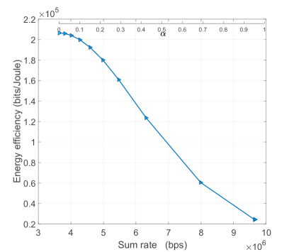
Figure 5: Pareto front of SE-EE trade-off-based design for TX-SNR = 24 dB.

V Conclusion

In this paper, we proposed a beamforming design that jointly considers the maximization of the conflicting performance metrics EE and SE. In particular, we formulate this challenging design problem through a weighted sum approach based on the priori articulation. However, this original problem is not convex due to non-convex multi-objective function and constraints. To overcome these non-convexity issues, we exploit the SCA technique to attain the solution. Furthermore, we show that the proposed approach achieves a Pareto-optimal solution. Simulation results have been provide to validate the effectiveness of the proposed algorithm and the performance is compared with a benchmark power minimization approach.

Appendix A

PROOF OF THEOREM 1

First, we denote the beamforming vectors that provide an optimal solution to $\overset{\sim}{OP}$ as ${\{\mathbf{w}_{i}^{*}\}_{i=1}^{K}}$. Therefore,

$$f_{EE-SE}({\{\mathbf{w}_{i}^{*}\}_{i=1}^{K}})\geq f_{EE-SE}({\{\mathbf{w}_{i}\}_{i=1}^{K}}),$$ (41)

which can be rewritten as

$$\sum_{l=1}^{2}\alpha_{l}f_{l}^{Norm}({\{\mathbf{w}_{i}^{*}\}_{i=1}^{K}})-\sum_{l=1}^{2}\alpha_{l}f_{l}^{Norm}({\{\mathbf{w}_{i}\}_{i=1}^{K}})\geq 0.$$ (42)

The inequality in (42) can be equivalently reformulated as

$$\sum_{l=1}^{2}\frac{\alpha_{l}}{f_{l}^{*}}(f_{l}({\{\mathbf{w}_{i}^{*}\}_{i=1}^{K}})-f_{l}({\{\mathbf{w}_{i}\}_{i=1}^{K}}))\geq 0.$$ (43)

In particular, we prove Theorem 1 by using a contradiction argument, as follows. First, we assume that $\{\mathbf{w}_{i}^{*}\}_{i=1}^{K}$ is not a Pareto-optimal solution to the original optimization problem ${OP}$. This assumption implies that there exists another feasible solution $\{\mathbf{w}_{i}^{{}^{\prime}}\}_{i=1}^{K}$ such that

$$\mathbf{f}{\{\mathbf{w}_{i}^{{}^{\prime}}\}_{i=1}^{K}}\succ\mathbf{f}{\{\mathbf{w}_{i}^{*}\}_{i=1}^{K}}.$$ (44)

The condition in (44) can be equivalently written as

$$(f_{l}({\{\mathbf{w}_{i}^{{}^{\prime}}\}_{i=1}^{K}})-f_{l}({\{\mathbf{w}_{i}^{*}\}_{i=1}^{K}}))>0,\forall l\in{1,2}.$$ (45)

Without loss of generality, each element in (45) can be scaled by a positive constant (i.e., $\frac{\alpha_{l}}{f_{l}^{*}},\forall l\in\{1,2\}$). Furthermore, both of these inequalities can be added

$$\sum_{l=1}^{2}\frac{\alpha_{l}}{f_{l}^{*}}(f_{l}({\{\mathbf{w}_{i}^{{}^{\prime}}\}_{i=1}^{K}})-f_{l}({\{\mathbf{w}_{i}^{*}\}_{i=1}^{K}}))>0,\forall l\in{1,2}.$$ (46)

However, the inequality in (46) contradicts the fact that ${\{\mathbf{w}_{i}^{*}\}_{i=1}^{K}}$ is the optimal solution of $\overset{\sim}{OP}$. Therefore, the optimal solution of $\overset{\sim}{OP}$ satisfies the Pareto-optimality condition, and hence, it gives the Pareto-solutions of the original SE-EE trade-off $OP$ problem. This completes the proof of Theorem 1. $\blacksquare$

Appendix B

PROOF OF LEMMA 1

Lemma 1 presents that $f_{1}^{Norm}$ and $f_{2}^{Norm}$ remain constant with the different weight factors while the available power is less than green power. This can be equivalently written as

$$\{f_{1}^{Norm}(\beta_{1})\}_{P_{ava}=P_{1}}=\{f_{1}^{Norm}(\beta_{2})\}_{P_{ava}=P_{1}},$$ (47a)

$$\{f_{2}^{Norm}(\beta_{1})\}_{P_{ava}=P_{1}}=\{f_{2}^{Norm}(\beta_{2})\}_{P_{ava}=P_{1}},$$ (47b)

where $P_{1}$ is less than the green power, and $\beta_{1},\beta_{2}\in[0,1]$. In order to prove this, we validate (47a) and (47b) with the extreme conditions of $\beta_{1}=0$ and $\beta_{2}=1$. We start with $\beta_{1}=0$, in which case ${\overset{\sim}{OP}}$ turns out to be an SE-Max problem, and thus, the maximum SE is achieved. Therefore,

$$\{f_{1}^{Norm}(\beta_{1}=0)\}_{P_{ava}=P_{1}}=1.$$ (48)

Furthermore, it has been already verified in [27] that both SE-Max and GEE-Max problem provide the same optimal beamforming vectors with an available power less than the green power. This means that $\{f_{2}(\beta_{1}=0)\}_{P_{ava}=P_{1}}=f_{2}^{*}$, therefore,

$$\{f_{2}^{Norm}(\beta_{1}=0)\}_{P_{ava}=P1}=1.$$ (49)

Similarly, we follow the same approach for the case with $\beta_{2}=1$, where ${\overset{\sim}{OP}}$ becomes the GEE-Max problem. The maximization of EE with an available power less than the green power will simultaneously achieve the maximum sum rate and the maximum EE. Hence,

$$\{f_{1}^{Norm}(\beta_{2}=1)\}_{P_{ava}=P_{1}}=1,$$ (50a)

$$\{f_{2}^{Norm}(\beta_{2}=1)\}_{P_{ava}=P_{1}}=1.$$ (50b)

It is can be easily noticed that (48), (49), (50a), and (50b) validate the conditions provided in (47a), (47b). This completes the proof of Lemma 1. $\blacksquare$

References

- [1] R. Vannithamby and S. Talwar, Towards 5G Applications: Requirements and Candidate Technologies. John Wiley & Sons, 2017.
- [2] P. Gandotra, R. K. Jha, and S. Jain, “Green communication in next generation cellular networks: A survey,” IEEE Access, vol. 5, pp. 11 727–11 758, Jun. 2017.
- [3] A. Zappone and E. Jorswieck, “Energy efficiency in wireless networks via fractional programming theory,” Found. Trends Commun. Inf. Theory, vol. 11, no. 3-4, pp. 185–396, Jan. 2015.
- [4] T. L. Marzetta, “Noncooperative cellular wireless with unlimited numbers of base station antennas,” IEEE Trans. Wireless Commun., vol. 9, no. 11, pp. 3590–3600, Nov. 2010.
- [5] M. Bashar, K. Cumanan, A. G. Burr, H. Q. Ngo, E. G. Larsson, and P. Xiao, “Energy efficiency of the cell-free massive MIMO uplink with optimal uniform quantization,” IEEE Trans. Green Commun. Netw., vol. 3, no. 4, pp. 971–987, Dec. 2019.
- [6] L. Zhu, J. Zhang, Z. Xiao, X. Cao, D. O. Wu, and X.-G. Xia, “Joint Tx-Rx beamforming and power allocation for 5G Millimeter-Wave non-orthogonal multiple access (MmWave-NOMA) Networks,” IEEE Trans. Commun., 2019.
- [7] Z. Xiao, L. Zhu, J. Choi, P. Xia, and X.-G. Xia, “Joint power allocation and beamforming for non-orthogonal multiple access (NOMA) in 5G millimeter wave communications,” IEEE Trans. Wireless Commun., vol. 17, no. 5, pp. 2961–2974, May 2018.
- [8] S. Tomida and K. Higuchi, “Non-orthogonal access with SIC in cellular downlink for user fairness enhancement,” in Proc. IEEE Inter. Symp. on Intell. Signal Process. and Comm. Sys. (ISPACS), 2011, 2011, pp. 1–6.
- [9] Y. Saito, Y. Kishiyama, A. Benjebbour, T. Nakamura, A. Li, and K. Higuchi, “Non-orthogonal multiple access (NOMA) for cellular future radio access,” in Proc. IEEE VTC Spring 2013, 2013, pp. 1–5.
- [10] Z. Ding, Y. Liu, J. Choi, Q. Sun, M. Elkashlan, I. Chih-Lin, and H. V. Poor, “Application of non-orthogonal multiple access in LTE and 5G networks,” IEEE Commun. Mag., vol. 55, no. 2, pp. 185–191, Feb. 2017.
- [11] S. Vanka, S. Srinivasa, Z. Gong, P. Vizi, K. Stamatiou, and M. Haenggi, “Superposition coding strategies: Design and experimental evaluation,” IEEE Trans. Wireless Commun., vol. 11, no. 7, pp. 2628–2639, Jul. 2012.
- [12] P. Xu, K. Cumanan, and Z. Yang, “Optimal power allocation scheme for NOMA with adaptive rates and alpha-fairness,” in Proc. IEEE GLOBECOM, 2017, pp. 1–6.
- [13] L. Lv, J. Chen, and Q. Ni, “Cooperative non-orthogonal multiple access in cognitive radio,” IEEE Commun. Lett., vol. 20, no. 10, pp. 2059–2062, Oct. 2016.
- [14] B. Wang, L. Dai, Z. Wang, N. Ge, and S. Zhou, “Spectrum and energy-efficient beamspace MIMO-NOMA for millimeter-wave communications using lens antenna array,” IEEE J. Sel. Areas Commun., vol. 35, no. 10, pp. 2370–2382, Oct. 2017.
- [15] Z. Wei, L. Zhao, J. Guo, D. W. K. Ng, and J. Yuan, “A multi-beam NOMA framework for hybrid mmwave systems,” in Proc. IEEE International Conference on Communications (ICC), 2018, pp. 1–7.
- [16] Q. Sun, S. Han, I. Chin-Lin, and Z. Pan, “On the ergodic capacity of MIMO NOMA systems,” IEEE Wireless Commun. Lett., vol. 4, no. 4, pp. 405–408, Aug. 2015.
- [17] Z. Chen, Z. Ding, P. Xu, and X. Dai, “Optimal precoding for a QoS optimization problem in two-user MISO-NOMA downlink,” IEEE Commun. Lett., vol. 20, no. 6, pp. 1263–1266, Jun. 2016.
- [18] M. Zhang, K. Cumanan, J. Thiyagalingam, W. Wang, A. G. Burr, Z. Ding, and O. A. Dobre, “Energy efficiency optimization for secure transmission in MISO cognitive radio network with energy harvesting,” IEEE Access, vol. 7, pp. 126 234–126 252, 2019.
- [19] X. Wei, H. Al-Obiedollah, K. Cumanan, M. Zhang, J. Tang, W. Wang, and O. A. Dobre, “Resource allocation technique for hybrid TDMA-NOMA system with opportunistic time assignment,” arXiv preprint arXiv:2003.02196, 2020.
- [20] Z. Ding, F. Adachi, and H. V. Poor, “The application of MIMO to non-orthogonal multiple access,” IEEE Trans. Wireless Commun., vol. 15, no. 1, pp. 537–552, Jan. 2016.
- [21] H. Sun, F. Zhou, R. Q. Hu, and L. Hanzo, “Robust beamforming design in a NOMA cognitive radio network relying on SWIPT,” IEEE Sel. Areas in Commun., vol. 37, no. 1, pp. 142–155, Jan. 2019.
- [22] F. Zhou, Z. Chu, H. Sun, R. Q. Hu, and L. Hanzo, “Artificial noise aided secure cognitive beamforming for cooperative MISO-NOMA using SWIPT,” IEEE Sel. Areas in Commun., vol. 36, no. 4, pp. 918–931, Apr. 2018.
- [23] F. Zhou, Z. Li, J. Cheng, Q. Li, and J. Si, “Robust AN-aided beamforming and power splitting design for secure MISO cognitive radio with SWIPT,” IEEE Trans Wireless Commun., vol. 16, no. 4, pp. 2450–2464, Apr. 2017.
- [24] Y. Liu, Z. Qin, M. Elkashlan, Z. Ding, A. Nallanathan, and L. Hanzo, “Non-orthogonal multiple access for 5G and beyond,” arXiv preprint arXiv:1808.00277, 2018.
- [25] F. Alavi, K. Cumanan, Z. Ding, and A. G. Burr, “Outage constraint based robust beamforming design for non-orthogonal multiple access in 5G cellular networks,” in Proc. IEEE 28th Annual International Symposium on Personal, Indoor, and Mobile Radio Communications (PIMRC), 2017, pp. 1–5.
- [26] M. F. Hanif, Z. Ding, T. Ratnarajah, and G. K. Karagiannidis, “A minorization-maximization method for optimizing sum rate in the downlink of non-orthogonal multiple access systems,” IEEE Trans. Signal Process., vol. 64, no. 1, pp. 76–88, Jan. 2016.
- [27] H. M. Al-Obiedollah, K. Cumanan, J. Thiyagalingam, A. G. Burr, Z. Ding, and O. A. Dobre, “Energy efficient beamforming design for MISO non-orthogonal multiple access systems,” IEEE Trans. Commun., vol. 67, no. 6, pp. 4117–4131, Jun. 2019.
- [28] H. Al-Obiedollah, K. Cumanan, J. Thiyagalingam, A. G. Burr, Z. Ding, and O. A. Dobre, “Energy efficiency fairness beamforming design for MISO NOMA systems,” in Proc. IEEE WCNC, 2019.
- [29] J. Lorincz and I. Bule, “Renewable energy sources for power supply of base station sites,” International Journal of Business Data Communications and Networking (IJBDCN), vol. 9, no. 3, pp. 53–74, 2013.
- [30] L.-C. Wang and S. Rangapillai, “A survey on green 5G cellular networks,” in Proc. International Conference on Signal Processing and Communications (SPCOM), 2012, pp. 1–5.
- [31] C. Xiong, G. Y. Li, S. Zhang, Y. Chen, and S. Xu, “Energy-and spectral-efficiency tradeoff in downlink OFDMA networks,” IEEE Trans. Wireless Commun., vol. 10, no. 11, pp. 3874–3886, Dec. 2011.
- [32] F. Alavi, K. Cumanan, M. Fozooni, Z. Ding, S. Lambotharan, and O. A. Dobre, “Robust energy-efficient design for miso non-orthogonal multiple access systems,” IEEE Transactions on Communications, vol. 67, no. 11, pp. 7937–7949, 2019.
- [33] L. Deng, Y. Rui, P. Cheng, J. Zhang, Q. Zhang, and M. Li, “A unified energy efficiency and spectral efficiency tradeoff metric in wireless networks,” IEEE Commun. Lett., vol. 17, no. 1, pp. 55–58, Jan. 2013.
- [34] A. Konak, D. W. Coit, and A. E. Smith, “Multi-objective optimization using genetic algorithms: A tutorial,” Reliability Engineering & System Safety, vol. 91, no. 9, pp. 992–1007, Sep. 2006.
- [35] A. Zhou, B.-Y. Qu, H. Li, S.-Z. Zhao, P. N. Suganthan, and Q. Zhang, “Multiobjective evolutionary algorithms: A survey of the state of the art,” Swarm and Evolutionary Computation, vol. 1, no. 1, pp. 32–49, Mar. 2011.
- [36] R. T. Marler and J. S. Arora, “Survey of multi-objective optimization methods for engineering,” Structural and Multidisciplinary Optimization, vol. 26, no. 6, pp. 369–395, Apr. 2004.
- [37] H. Al-Obiedollah, K. Cumanan, J. Thiyagalingam, A. G. Burr, Z. Ding, and O. A. Dobre, “Sum rate fairness trade-off-based resource allocation technique for MISO NOMA systems,” in Proc. IEEE WCNC, 2019.
- [38] O. Amin, E. Bedeer, M. H. Ahmed, and O. A. Dobre, “Energy efficiency–spectral efficiency tradeoff: A multiobjective optimization approach,” IEEE Trans. Veh. Technol., vol. 65, no. 4, pp. 1975–1981, Apr. 2016.
- [39] E. Bedeer, O. A. Dobre, M. H. Ahmed, and K. E. Baddour, “A multiobjective optimization approach for optimal link adaptation of OFDM-based cognitive radio systems with imperfect spectrum sensing,” IEEE Trans. Wireless Commun., vol. 13, no. 4, pp. 2339–2351, Apr. 2014.
- [40] W. Zhang, C.-X. Wang, D. Chen, and H. Xiong, “Energy–spectral efficiency tradeoff in cognitive radio networks,” IEEE Trans. Veh. Technol., vol. 65, no. 4, pp. 2208–2218, May 2015.
- [41] X. Hong, Y. Jie, C.-X. Wang, J. Shi, and X. Ge, “Energy-spectral efficiency trade-off in virtual MIMO cellular systems,” IEEE Sel. Areas in Commun., vol. 31, no. 10, pp. 2128–2140, Sep. 2013.
- [42] G. Liu and D. Jiang, “5G: Vision and requirements for mobile communication system towards year 2020,” Chinese Journal of Engineering, vol. 2016, Mar. 2016, Art. no. 5974586.
- [43] F. Alavi, K. Cumanan, Z. Ding, and A. G. Burr, “Beamforming techniques for non-orthogonal multiple access in 5G cellular networks,” IEEE Trans. Veh. Technol., vol. 67, no. 10, pp. 9474–9487, Oct. 2018.
- [44] P. Xu and K. Cumanan, “Optimal power allocation scheme for non-orthogonal multiple access with -fairness,” IEEE J. Sel. Areas in Commun., vol. 35, no. 10, pp. 2357–2369, Oct. 2017.
- [45] S. R. Islam, N. Avazov, O. A. Dobre, and K.-S. Kwak, “Power-domain non-orthogonal multiple access (NOMA) in 5G systems: Potentials and challenges,” IEEE Commun. Surveys Tuts., vol. 19, no. 2, pp. 721–742, Oct. 2017.
- [46] M. Vaezi, R. Schober, Z. Ding, and H. V. Poor, “Non-orthogonal multiple access: Common myths and critical questions,” IEEE Wireless Communications, vol. 26, no. 5, pp. 174–180, 2019.
- [47] M. Zhang, K. Cumanan, and A. Burr, “Secure energy efficiency optimization for MISO cognitive radio network with energy harvesting,” in Proc. IEEE 9th International Conference on Wireless Communications and Signal Processing (WCSP), 2017, pp. 1–6.
- [48] M. Zeng, A. Yadav, O. A. Dobre, and H. V. Poor, “Energy-efficient power allocation for MIMO-NOMA with multiple users in a cluster,” IEEE Access, vol. 6, pp. 5170–5181, Feb. 2018.
- [49] S. Islam, M. Zeng, O. A. Dobre, and K.-S. Kwak, “Resource allocation for downlink NOMA systems: Key techniques and open issues,” IEEE Wireless Commun., vol. 25, no. 2, pp. 40–47, Apr. 2018.
- [50] A. Beck, A. Ben-Tal, and L. Tetruashvili, “A sequential parametric convex approximation method with applications to nonconvex truss topology design problems,” J. Global Optimiz., vol. 47, no. 1, pp. 29–51, May 2010.
- [51] H. Al-Obiedollah, K. Cumanan, A. G. Burr, J. Tang, Y. Rahulamathavan, Z. Ding, and O. A. Dobre, “On energy harvesting of hybrid TDMA-NOMA systems,” in Proc. IEEE Global Communications Conference (GLOBECOM), 2019, pp. 1–6.
- [52] S. Boyd and L. Vandenberghe, Convex Optimization. Cambridge Univ. Press, 2004.
- [53] M. Bengtsson and B. Ottersten, “Optimal downlink beamforming using semidefinite optimization,” in Proc. Annual Allerton Conf. on Commun., Control and Computing, 1999, pp. 987–996.
- [54] K. Cumanan, L. Musavian, S. Lambotharan, and A. B. Gershman, “Sinr balancing technique for downlink beamforming in cognitive radio networks,” IEEE Signal Processing Letters, vol. 17, no. 2, pp. 133–136, 2010.
- [55] F. Alavi, K. Cumanan, Z. Ding, and A. G. Burr, “Robust beamforming techniques for non-orthogonal multiple access systems with bounded channel uncertainties,” IEEE Commun. Lett., vol. 21, no. 9, pp. 2033–2036, Sept. 2017.
- [56] K. Cumanan, R. Krishna, L. Musavian, and S. Lambotharan, “Joint beamforming and user maximization techniques for cognitive radio networks based on branch and bound method,” IEEE Trans. Wireless Commun., vol. 9, no. 10, pp. 3082–3092, Oct. 2010.
- [57] Y. Nesterov and A. Nemirovskii, Interior-point Polynomial Algorithms in Convex Programming. Philadelphia, PA: SIAM, 1994.
- [58] M. S. Lobo, L. Vandenberghe, S. Boyd, and H. Lebret, “Applications of second-order cone programming,” Linear Algebra and its Appl., vol. 284, pp. 193–228, Nov. 1998.
- [59] M. Grant, S. Boyd, and Y. Ye, “CVX: Matlab software for disciplined convex programming,” 2008.