An Online Matching Model for
Self-Adjusting ToR-to-ToR Networks

Abstract.

This is a short note that formally presents the matching model for the theoretical study of self-adjusting networks as initially proposed in (avin2019toward, ).

1. Background and Motivation

This note is motivated by the observation that existing datacenter network designs sometimes provide a mismatch between some common traffic patterns and the switching technology used in the network topology to serve it. On the contrary, we make the case for a systematic approach to assign a specific type of traffic or flow to the topology component which best matches its characteristics and requirements. For instance, static topology components can provide a very low latency, however, static topologies inherently require multi-hop forwarding: the more hops a flow has to traverse, the more network capacity is consumed, which can be seen as an “bandwidth tax,” as noticed in prior work (rotornet, ). This makes these networks less fitted at high loads: the more traffic they carry, the more bandwidth tax is paid. Inspired by the notion of bandwidth tax, we introduce a second dimension, called “latency tax” to capture the delay incurred by the reconfiguration time of optical switches. For instance, rotor switches reduce the bandwidth tax by providing periodic direct connectivity. While this architecture performs well for all-to-all traffic patterns, it is less suited for elephant flows created by ring-reduce traffic pattern of machine learning training with Horovod. We note that static and rotor topology components both form demand-oblivious topologies, and hence, they cannot account for specific elephant flows. While Valiant routing (valiant1982scheme, ) can be used in combination with rotor switches to carry large flows, this again results in bandwidth tax. This is the advantage of demand-aware topologies, based on 3D MEMS optical circuit switches, which can provide shortcuts specifically to such elephant flows. However, the state-of-the-art demand-aware optical switches have a reconfiguration latency of several milliseconds and hence incur a higher latency tax to establish a circuit. Moreover, demand-aware topologies might require a control logic that adds to the latency tax. Thus, this latency can only be amortized for large flows, which benefit from the demand-aware topology components in the longer term.

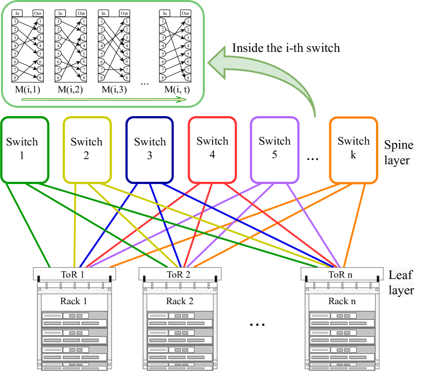
Figure 1. Overview of TMT model.

2. ToR-Matching-ToR Architecture

Given the above motivation for a unified network design, combining the advantages of static, rotor, and demand-aware switches, we propose a two-layer leaf-spine network architecture in which spine switches can be of different types Static, Rotor and Demand-aware. Since this network architecture generalizes existing architectures such as RotorNet (rotornet, ), in that it supports different types of switches matching ToRs to each other, we will refer to it as the ToR-Matching-ToR (TMT) network model.

More specifically, the TMT network interconnects a set of $n$ ToRs, $\{1,2,\dots,n\}$ and its two-layer leaf-spine architecture composed of leaf switches and spine switches, similar to (opera, ; rotornet, ). The $n$ ToR packet switches are connected using $k$ spine switches, $SW=\{sw_{1},sw_{2},\dots,sw_{k}\}$ and each switch internally connects its in-out ports via a matching. Figure 1 illustrates a schematic view of our design. We assume that each ToR $i:1\leq i\leq n$ has $k$ uplinks, where uplink $j:1\leq j\leq k$ connects to port $i$ in $sw_{j}$. The directed outgoing (leaf) uplink is connected to incoming port of the (spine) switch and the directed incoming (leaf) uplink is connected to the outgoing port of the (spine) switch. Each switch has $n$ input ports and $n$ output ports and the connections are directed, from input to output ports.

At any point in time, each switch $sw\in SW$ provides a matching between its input and output ports. Depending on the switch type, this matching may be reconfigured at runtime: The set of matchings $\mathcal{M}_{j}$ of a switch $j$ may be larger than one, i.e., $m_{j}=\lvert\mathcal{M}_{j}\rvert>1$. Changing from a matching $M^{\prime}\in\mathcal{M}$ to a matching $M^{\prime\prime}\in\mathcal{M}$ takes time, which we model with a parameter $R_{j}$: the reconfiguration time of switch $j$. During reconfiguration, the links in $M^{\prime}\cap M^{\prime\prime}$, i.e., the links which are not being reconfigured, can still be used for forwarding; the remaining links are blocked during the reconfiguration. Depending on the technology, different switches in $SW$ support different sets of matchings and reconfiguration times.

We note that the TMT network can be used to model existing systems, e.g., Eclipse (venkatakrishnan2018costly, ) or ProjecToR (projector, ) which rely on a demand-aware switches, RotorNet (rotornet, ) and Opera (opera, ) which relies on a rotor based switches, or an optical variant of Xpander (xpander, ) which can be built from a collection of static matchings.

3. The Matching Model

This section presents a general algorithmic model for Self-Adjusting Networks (SAN) constructed using a set of matchings. We mostly follow (avin2019toward, ). We consider a set of $n$ nodes $V=\{1,\ldots,n\}$ (e.g., the top-of-rack switches). The communication demand among these nodes is a sequence $\sigma=(\sigma_{1},\sigma_{2},\ldots)$ of communication requests where $\sigma_{t}=(u,v)\in V\times V$, is a source-destination pair. The communication demand can either be finite or infinite.

In order to serve this demand, the nodes $V$ must be inter-connected by a network $N$, defined over the same set of nodes. In case of a demand-aware network, $N$ can be optimized towards $\sigma$, either statically or dynamically: a self-adjusting network $N$ can change over time, and we denote by $N_{t}$ the network at time $t$, i.e., the network evolves: $N_{0},$ $N_{1},$ $N_{2},$ $\ldots$

3.1. Matching

The $n$ nodes are connected using $k$ switches, $SW=\{sw_{1},sw_{2},\dots,sw_{k}\}$ and each switch internally connects its $n$ in-out ports via a matching. These matchings can be dynamic, and change over time. To denote the matching on a switch $i$ at time $t$ we use $M(i,t)$. At each time $t$ our network is the union of these matchings, $N_{t}=\mathcal{M}=\bigcup_{i=1}^{k}M(i,t)$.

In general, not all switches are necessarily reconfigurable. Since, reconfigurable switches tend to be more costly than static ones, a network could gain from using some hybrid mix of switches.

3.2. Cost

The crux of designing smart self-adjusting networks is to find an optimal tradeoff between the benefits and the costs of reconfiguration: while by reconfiguring the network, we may be able to serve requests more efficiently in the future, reconfiguration itself comes at a cost.

The inputs to the matching based self-adjusting network design problem is the number of nodes $n$, the number of switches (i.e., matchings) $k$, a set of allowed network topologies $\mathcal{N}$ (i.e., all networks that can be built from $k$ matchings), the request sequence $\sigma=(\sigma_{1},\sigma_{1},\ldots,\sigma_{m})$, and two types of costs:

• An adjustment cost $\mathrm{adj}:\mathcal{N}\times\mathcal{N}\rightarrow\mathbb{R}$ which defines the cost of reconfiguring a network $N\in\mathcal{N}$ to a network $N^{\prime}\in\mathcal{N}$. Adjustment costs may include mechanical costs (e.g., energy required to move lasers or abrasion) as well as performance costs (e.g., reconfiguring a network may entail control plane overheads or packet reorderings, which can harm throughput). For example, the cost could be given by the number of links which need to be changed in order to transform the network.

• A service cost $\mathrm{srv}:\sigma\times\mathcal{N}\rightarrow\mathbb{R}$ which defines, for each request $\sigma_{i}$ and for each network $N\in\mathcal{N}$, what is the price of serving $\sigma_{i}$ in network $N$. For example, the cost could correspond to the route length: shorter routes require less resources and hence reduce not only load (e.g., bandwidth consumed along fewer links), but also energy consumption, delay, and flow completion times, could be considered for example.

Serving request $\sigma_{i}$ under the current network configuration $N_{i}$ will hence cost $\mathrm{srv}(\sigma_{i},N_{i})$, after which the network reconfiguration algorithm may decide to reconfigure the network at cost $\mathrm{adj}(N_{i},N_{i+1})$. The total processing cost of a demand sequence $\sigma$ for an algorithm $\mathcal{A}$ is then

(1) $$\mathrm{Cost}(\mathcal{A},N_{0},\sigma)=\sum_{t=1}^{m}\mathrm{srv}(\sigma_{t},N_{t-1})+\mathrm{adj}(N_{t-1},N_{t})$$

where $N_{t}\in\mathcal{N}$ denotes the network at time $i$.

3.3. Specific Metrics

3.3.1. Service Cost

In order to give a more useful description of the performance of a self-adjusting network, we model the service cost for each $\sigma_{i}=(u,v)$ as the shortest distance between $u$ and $v$ on the graph $N_{i}$, that is

$$\mathrm{srv}(\sigma_{t},N_{t})=d_{N_{t}}(u,v)=d(\sigma_{t},N_{t})$$

where $d_{G}(u,v)$ denotes the shortest path distance between $u$ and $v$ on the graph $G$.

3.3.2. Adjustments Cost

Adjustments cost can depend on the particular network modeled. We will discuss three particular cases for adjustment costs and recall that our network graph at time $t$, $N_{t}$, is a union of the different matchings on each of our $k$ switches. At any time $t$, a switch can adjust its matching, causing a change in the overall network’s topology.

• Edge Distance: The basic case where we define the adjustments cost as propositional to the number of replaced edges between each consecutive matchings of the same switch. Recall that we denote the matching of switch $i$ at time $t$ as $M(i,t)$, which denotes the set edges in the the matching. Let the cost of a single edge be $\alpha$ then the adjustment cost for a single switch is therefore $\alpha\cdot\lvert M(i,t+1)\setminus M(i,t)\rvert$, where $S\setminus T$ denotes the set difference between $S$ and $T$. For the entire network, this turns out to be

  $$\mathrm{adj}(N_{t-1},N_{t})=\alpha\sum_{i=1}^{k}\lvert M(i,t)\setminus M(i,t-1)\rvert.$$

• Switch Cost: In this case, if a matching (switch) is changed, it costs $\alpha$ regardless of the number of edge changes in the matching. Let $\mathbb{I}_{S=T}$ be an indicator function that denotes if set $S$ is equal set $T$. Then the adjustments cost for the network is:

  $$\mathrm{adj}(N_{t-1},N_{t})=\alpha\sum_{i=1}^{k}\mathbb{I}_{M(i,t)=M(i,t-1)}.$$

• No Direct Cost: In this case the adjustment cost is zero

  $$\mathrm{adj}(N_{t-1},N_{t})=0$$

  however the cost of reconfiguring the network is still incurred through the inactivity of some of the edges during the adjustment itself. When some switch $i$ changes its matching from $M(i,t)$ to $M(i,t+1)$, its edges will be unavailable, and requests cannot be served using these edges until the adjustment process is completed after some $\beta$ units of time. Here, we also consider two cases: (i) the entire switch (matching) is unavailable for $\beta$ time units, namely all its edges are inactive; (ii) only the edges that are changing are inactive for $\beta$ time units. Let $M^{*}(i,t)$ denote the set of active edges in matching $M(i,t)$ (or in $sw_{i}$). Then for each time $t$ we have:

  $$N_{t}=\bigcup_{i=1}^{k}M^{*}(i,t)$$

References

- (1) C. Avin and S. Schmid, “Toward demand-aware networking: A theory for self-adjusting networks,” ACM SIGCOMM Computer Communication Review, vol. 48, no. 5, pp. 31–40, 2019.
- (2) W. M. Mellette, R. McGuinness, A. Roy, A. Forencich, G. Papen, A. C. Snoeren, and G. Porter, “Rotornet: A scalable, low-complexity, optical datacenter network,” in Proceedings of the Conference of the ACM Special Interest Group on Data Communication, pp. 267–280, ACM, 2017.
- (3) L. G. Valiant, “A scheme for fast parallel communication,” SIAM journal on computing, vol. 11, no. 2, pp. 350–361, 1982.
- (4) W. M. Mellette, R. Das, Y. Guo, R. McGuinness, A. C. Snoeren, and G. Porter, “Expanding across time to deliver bandwidth efficiency and low latency,” arXiv preprint arXiv:1903.12307, 2019.
- (5) S. B. Venkatakrishnan, M. Alizadeh, and P. Viswanath, “Costly circuits, submodular schedules and approximate carathéodory theorems,” Queueing Systems, vol. 88, no. 3-4, pp. 311–347, 2018.
- (6) M. Ghobadi, R. Mahajan, A. Phanishayee, N. Devanur, J. Kulkarni, G. Ranade, P.-A. Blanche, H. Rastegarfar, M. Glick, and D. Kilper, “Projector: Agile reconfigurable data center interconnect,” in Proceedings of the 2016 ACM SIGCOMM Conference, pp. 216–229, ACM, 2016.
- (7) S. Kassing, A. Valadarsky, G. Shahaf, M. Schapira, and A. Singla, “Beyond fat-trees without antennae, mirrors, and disco-balls,” in Proceedings of the Conference of the ACM Special Interest Group on Data Communication, pp. 281–294, ACM, 2017.