Additive Partial Matchings Induced by Persistence Morphisms
Abstract
Given a morphism of persistence modules (a.k.a. persistence morphism) , we introduce a novel operator that determines a partial matching between the barcodes of and induced by . We show that the proposed operator is additive with respect to the direct sum of persistence morphisms, and that it contains more information than and the rank invariant. We also illustrate some advantages of using our induced partial matching over the Bauer-Lesnick partial matching . Lastly, we provide a family of persistence morphisms that contain modules built from Morse filtrations, for which , the rank invariant and our proposed induced partial matching are equivalent.
1 Introduction
Persistence modules (PMs) have been extensively used to study persistent homology, one of the main tools of Topological Data Analysis (TDA). Morphisms of PMs (so-called persistence morphisms) appear in different settings, for example, when calculating the persistent homology of the Vietoris-Rips filtrations of two point clouds, one embedded into the other.
Informally, a PM is defined as a finite sequence of finite dimensional vector spaces over a fixed field and linear maps between them,
A persistence morphism between two PMs and is a finite set of linear maps for , making the following diagram commutative
| (1) |
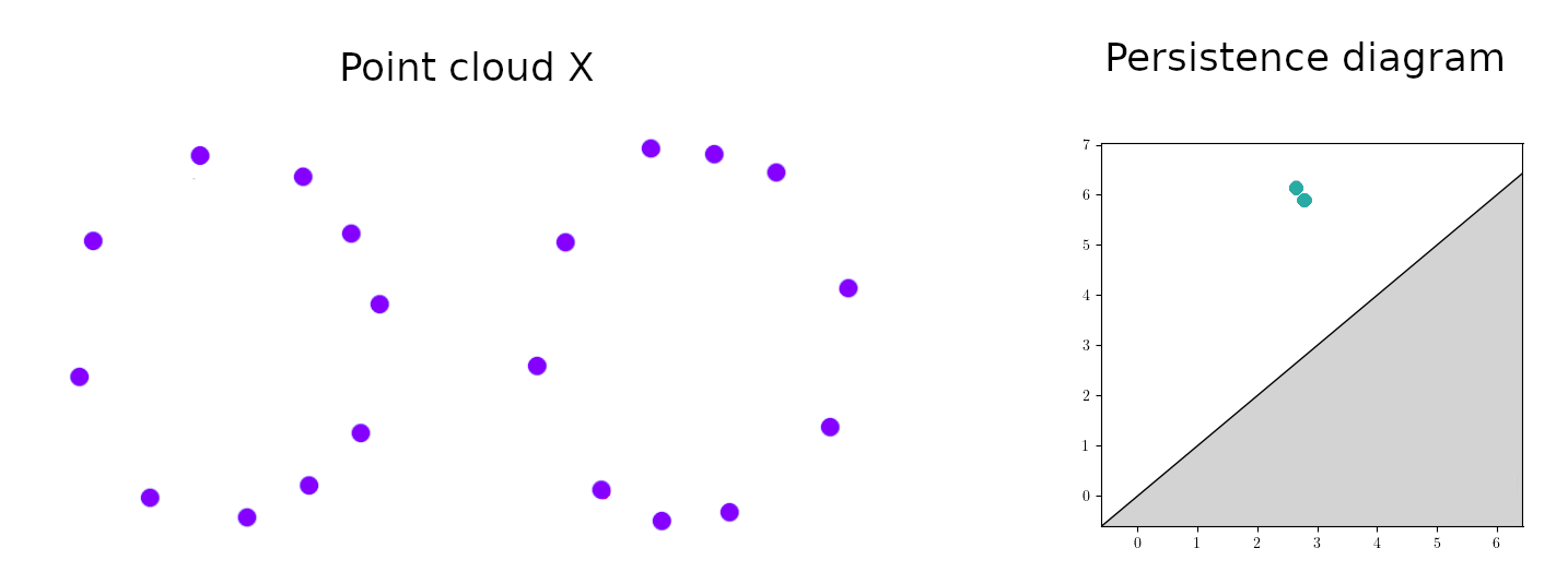
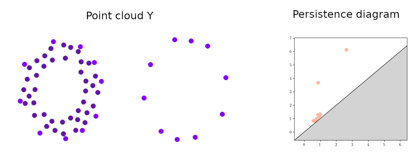
The structure theorem [1, 2] states that PMs can always be described using a multiset of intervals with an associated multiplicity known as persistence diagram (PD). In practice, PDs are plotted in the plane, with the intervals depicted as points. PDs help researchers to gain insight into the topological structure of data [3]. The usual pipeline is the following: First, a nested sequence of simplicial complexes is obtained from the point cloud using, for example, the Vietoris-Rips filtration. Then, the homology functor is used to obtain a vector space from each of these complexes and linear maps between them, leading to a PM. The intuition is that the further a point in the plot of the PD is from the diagonal line , the more important the homology feature it represents. See Figure 1 for an example.
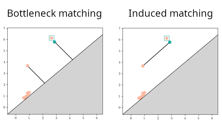
If we denote the PMs obtained from the point clouds and pictured in Figure 1 as and , we can use the inclusion to obtain a persistence morphism [4]. Our intuition from the point clouds says that both and represent two circles, one on the left and one on the right. These circles are represented in the PD plot by the points that are further from the diagonal. What is more, from the visual intuition, our aim is to obtain a partial matching induced from to identify the right (resp. left) circle in with the right (resp. left) circle in . In practice, PDs are compared using the bottleneck distance [3, 2], which is defined using partial matchings (partial bijections between intervals). More precisely, the bottleneck distance is defined using a partial matching that minimizes the supremum distance between the points representing the matched intervals as well as the distance to the diagonal of the points representing the unmatched intervals. Note that the partial matching used to define the bottleneck distance may not be the expected partial matching from the function , see Figure 2.
We define a method to obtain partial matchings from persistence morphisms satisfying some desirable properties, like being additive with respect to the direct sum of persistence morphisms. We also prove that it is richer than other invariants used to study , like the rank invariant or the image persistence module . In the rest of this section, we motivate the problem, relate our construction with other TDA concepts, and explain further the aforementioned properties.
1.1 Decomposition of persistence morphisms
Persistence morphisms with the structure displayed in diagram (1) belong to a more general class of PMs called ladder modules [5]. An important property of ladder modules is that they can be uniquely described, up to isomorphism, as direct sums of indecomposable ladder modules [5], as illustrated in the following example.
Example 1.1.
The following persistence morphism
is isomorphic to the following direct sum of indecomposable persistence morphisms
In Example 1.1, the intervals of the PD of are and ; while the PD of has a single interval with multiplicity . From the decomposition of , we deduce that a partial matching induced by should be as follows:
Note that, when the indecomposable persistence morphisms have a simple form as in the previous example, we can deduce directly a partial matching induced by the persistence morphism from its decomposition [6]. However, as the following example shows, there are also more complex indecomposable persistence morphisms that do not clearly determine a partial matching.
Example 1.2.
The following persistence morphism is an indecomposable persistence morphism,
In this case, there is not a clear way of inducing a partial matching from , as there was in Example 1.1
Moreover, the set of indecomposable ladder modules (including persistence morphisms) is wild for [5], which means that calculating the decomposition of a ladder module is very challenging.
1.2 Persistence morphism invariants
Since calculating the decomposition of a persistence morphism is generally impractical, we need to find other ways to study . One possibility is the rank invariant [7], given by the rank of the linear maps between all possible pairs of vector spaces in Diagram 1. Another possibility is to calculate the image persistence module [4], given by the following submodule of ,
As we will see, our induced partial matching provides in general richer information than these invariants.
There exist other induced partial matchings in the literature. The one that appeared first is the Bauer-Lesnick induced partial matching , which uses a combinatorial construction to match points from the PD of with points of the PD of , and points of the PD of with points of the PD of . The virtue of is that it is fast to calculate and provides a constructive proof of the stability theorem [8, 9]. However, its output sometimes contradicts the intuition. For instance, if is the persistence morphism from Example 1.1, then induces the partial matching
instead of the expected partial matching described in Example 1.1. On the contrary, our proposed operator gives the expected partial matching as explained in Example 6.2.
Some other partial matchings induced by persistence morphisms have been independently proposed: the cycle registration method [10] and the cohomological cycle matching [11]. The first procedure is defined for the concrete case of Morse filtrations (see Section 6). The second is a generalization based on the concept of essential filtered complexes. Both of these matchings are defined for two facing persistence morphisms . On the contrary, our matching is defined for but does not require any additional restriction on .
An alternative construction to relate persistence diagrams is the persistent extensions introduced in [12], although this procedure is based on the witness complex and the Functorial Dowker Theorem, and then have different properties to ours [12]. Notice that [12] and [11] cite our previous preprint version [13].
Another related concept is the block function introduced by the authors of this paper in [14]. A block function can be seen as a weaker version of a partial matching. In [14] we showed that is additive with respect to the direct sum of persistence morphisms, so, when used in from Example 1.1 the output of corresponds with the intuition,
However, the block function does not always determine a unique partial matching. For instance, if is the persistence morphism given in Example 1.2, then from we deduce the following assignment
| (2) |
that is not a partial matching. We will see later that the method proposed in this paper always induces a unique partial matching for each .
All of these constructions are strongly related to persistence basis calculation and ladder module decomposition, see [15, 16, 17, 18, 19]. An exhaustive study of the relation between all these papers, including our construction, is out of the scope of this work. Hence, we limit to study in detail the relation with the most used partial matching, the proposed by Bauer and Lesnick, and with our previous work, the block function .
1.3 Results presented in this paper
We propose a new way of computing a partial matching between barcodes induced by a persistence morphism , based on a newly defined block function , and prove that and the rank invariant can be calculated from it. We also show that is additive with respect to the direct sum of persistence morphisms and it always induces a unique partial matching between the intervals of and . In addition, we provide an algorithm to compute and compare the induced block function to .
The paper is structured as follows. We introduce the background necessary in Section 2, and important operators used in the rest of the paper in Section 3. The definition of the block function and the proof that it induces a unique partial matching is provided in Section 4. In Section 5, we show how can be obtained from . The additivity of and its relation with the rank invariant are given in Section 6. In particular, we prove that the rank invariant can be calculated from . In Section 7, we provide a family of persistence morphisms where , and the rank invariant are equivalent. The algorithm for calculating by means of Gaussian reductions is given in Section 8. Finally, in Section 9, we study the relation between the proposed and the block function introduced in [14], and indicate how a combination of both can be used to understand the inner structure of the persistence morphisms. We end the paper with the conclusions and future works. Some technical lemmas can be found in two appendices, ensuring they do not disrupt the flow of the arguments contained in the paper.
| Persistence module (PM) | |
|---|---|
| Intervals | , |
| Interval modules | |
| Persistence diagram (PD) | |
| Barcode | |
| Persistence basis | |
| Persistence generator | |
| Persistence morphism | |
| Partial matching | |
| Induced block function |
2 Background
In this section, we provide the notions and preliminary results needed to understand the rest of the paper. For a more general introduction to persistent modules, please consult [2].
2.1 Persistence modules
All vector spaces considered in this paper are defined over a fixed field with a unit denoted by . Given , the expression denotes the set of integers . A persistence module (PM) indexed by the set consists of, a finite set of vector spaces for , and a set of linear maps for and ; such that if and is the identity map. The maps are known as the structure maps of and are denoted simply by when no confusion arises. To simplify notation, we add, to each PM, the trivial vector spaces as well as the respective trivial structure maps and for .
Given and in such that , we write to denote the interval set , and to denote all the intervals that are subsets of [n]. The interval module is composed by for all and otherwise, while the structure maps are given by the identity map whenever possible and the zero map otherwise.
In the following, we always denote the structure maps of the PMs and as and , respectively. The persistence module is a submodule of if for all and for any pair . The direct sum of and , , is defined using the vector spaces and the structure maps . If is a submodule of , the quotient is the persistence module whose vector spaces are for all and whose linear maps are induced by the structure maps from .
The following theorem states that any persistence module can be decomposed as a direct sum of interval modules.
Theorem 2.1 ([1]).
If is a PM then there exists a set of intervals and integers such that
As anticipated in Section 1, a persistence morphism is a set of linear maps , making the following diagram commutative,
The persistence morphism is an isomorphism/surjection/injection of PMs when all are isomorphisms/surjections/injections of vector spaces for . We omit the subindices of the linear map when these are clear from the context, for example, we might write instead of .
2.2 Persistence diagrams and barcodes
A multiset is a set where each element has associated a multiplicity, . The representation of a multiset, is the set defined by
The size of coincides with the size of its representation as calculated using the following formula,
Theorem 2.1 states that any PM can be defined, up to isomorphism, by pairs of intervals and multiplicities, i.e. using a multiset of intervals. Such multiset is called the persistence diagram (PD) of , and is denoted as . We denote the set of intervals in as and its representation as the barcode of , . PDs are plotted depicting the intervals as points in the plane with an index representing their multiplicity [3]. The multiplicity index might be dropped when it is not important for the representation, as in Figure 1. Be aware that, although persistence diagrams and barcodes are often considered equivalent, this paper uses persistence diagrams for multisets and barcodes for their representations.
In the following, we write the elements of as instead of . If is the only copy of the interval in the barcode, we might just write instead of . We also write to specify that the multiplicity of corresponds to the decomposition of , and we fix for .
Example 2.2.
The PD of and in Example 1.1 are and respectively. Their barcodes are and .
2.3 Persistence bases
A basis for [15, 2] is an isomorphism
with for all ; such isomorphism always exists by Theorem 2.1. The persistence generator is defined as the persistence morphism restricted to for . When we write , we mean that is the domain of . We also specify a persistence basis by its set of persistence generators .
Example 2.3.
Consider the PM given in Example 1.2. Since then is a basis for and the persistence generators and are given by the following commutative diagrams
Definition 2.4.
Given a subset of a persistence basis , we define the span of , denoted by , as the image of the sum of persistence generators in , that is
For , we define where stands for . In particular, and , where and are linearly independent sets of vectors in .
We use the following subsets of to characterize some spaces in the next subsection,
-
•
,
-
•
,
-
•
,
-
•
,
and write and instead of and .
2.4 Image and kernel operators of PMs
The operators , defined for fixed , were used in [1] to prove Theorem 2.1 and in [14], to define the block function . Since we need these operators to introduce , we recall their definition and provide an interpretation of them in terms of bases:
When or are fixed, and are PMs. The following lemma gives an intuitive idea of their structure:
Lemma 2.5 ([14]).
For any , , we have the equalities:
-
•
for all
-
•
for all .
The following trivial property will be important in further sections.
Lemma 2.6.
If then, and .
We combine these PMs to create new ones associated with intervals .
Furthermore, the previous operators can be described in terms of subsets of :
Lemma 2.7 ([14]).
We have that and for any .
Remark 2.8.
The previous lemma implies that for any . Then, provide all the information necessary to compute the decomposition of . An additional consequence is that for , .
Example 2.9.
Consider the following PM from Example 1.2,
We have , , and . Altogether we obtain that and . Additionally, one might check that for all . Then, .
2.5 Sections
Sections are the main algebraic tools used in [1] to prove Theorem 2.1. We recall their definition and properties here, and provide a sketch of their role in the proof to illustrate their use.
A section of a vector space is a pair of vector spaces such that . We say that a set of sections of with index set is disjoint if, for all , either or . It is said that it covers provided that for any subspace with there is some satisfying that
Theorem 2.10.
Let be a vector space and let be a disjoint set of sections of . Then
Particularly, if the set of sections is disjoint and covers then
Proof.
In order to prove Theorem 2.1, the author of [1] defined for each and , and proved that
-
•
is a disjoint set of sections that covers , and
-
•
for each and some .
Then, from Theorem 2.10, we deduce the isomorphisms
and the fact these structure maps of commute with these isomorphisms concludes the proof.
To prove that compose a set of sections that covers , an additional concept was used in [1] which we introduce next. A set of sections strongly covers a vector space provided that for all subspaces with there is some with
We can combine a set that strongly covers with one that covers to produce a new set that covers , see Lemma B.1. Lastly, we have added some technical lemmas about sections to Appendix B.
2.6 Partial matchings and block functions
A block function [14] between and is a function satisfying that if or and
| (3) |
A partial matching between two barcodes and is a bijection where and . Given two partial matchings between and , and , we say that and are isomorphic if there exist bijections making the following diagram commutative
and such that if then or then . By abuse of notation, we may write instead of , instead of , and say or when we mean .
Notice that for each partial matching, we can define a block function
that satisfies the additional property
| (4) |
And vice versa, a block function satisfying inequalities Eq. (3) and Eq. (4) determines a unique (up to isomorphism) partial matching between two barcodes, assigning copies of the interval to copies of the interval .
Example 2.11.
Given the barcodes and , the partial matchings
and
are isomorphic and define the same block function,
and for any other .
2.6.1 The induced partial matching
Firstly, given , denote by the subset of formed by the elements such that has as its right endpoint, and similarly, contains if is the left endpoint of . Observe that we can fix an order in each of these sets, for , if or and ; and for , if or and . The definition of is based on the following result.
Theorem 2.12 (Theorem 4.2 from [8]).
If is injective, then for each we have that
and if is surjective, then
Now observe that, given , there exists a unique decomposition where is surjective and is injective [8, 9]. Applying the previous theorem, we have that for each . Using the defined order for these sets, we can build a partial matching that maps the -th element of to the -th element of for all . This way, all the bars in are matched. Analogously, we can match the -th element of to the -th element of , obtaining a partial matching . Again, notice that all the bars in are matched. Then, a partial matching between and can be built concatenating and .
Remark 2.13.
A consequence of how is constructed is that, for each element in , there must be another element in with the same left endpoint and another element in with the same right endpoint, so that and .
Example 2.14.
Going back to Example 1.1, where
it can be checked that . Note now that the order in establishes that , and the one in establishes that . Then, the partial matching is given by
As we explained in the introduction, the partial matching in Example 2.14 is not compatible with the decomposition of the persistence morphism (see Example 1.1). With our porpoosed induced partial matching, we overcome this limitation. Moreover, in Section 7 we present a class of persistence morphisms for which , the rank invariant and our proposed induced partial matching are equivalent.
2.7 The induced block function
In [14], we defined a block function induced by a persistence morphism that is the precedent of the new induced block function , defined in Section 4. The block function is built from the PM , defined for each , using the vector spaces
if and otherwise, while the structure maps are induced by the quotient.
The induced block function is defined as:
for and .
Remark 2.15.
was defined in [14] as . However, is known to be unless , and since in this paper all intervals are closed, the direct limit is reduced to .
3 Interval blocks constructed using disjoint covering sets of sections
At the end of Section 1, we mentioned that the block function does not determine a unique partial matching in general. As pointed out by Corollary 5.6 of [14], this only happens if there are nested intervals in ; this is the case of Example 1.2. The root of this problem lies in the fact that, whenever there are nested intervals in , the sections may fail to be disjoint, as it is shown in the following example.
Example 3.1.
To obtain a disjoint set of sections, we use the following definitions based on the terms defined in Section 7 of [1].
Definition 3.2.
Let . Let us define the following PMs,
Example 3.3.
Next, we prove that and constitute disjoint sets of sections and their quotients are isomorphic to .
Proposition 3.4.
and are disjoint sets of sections that cover .
Proof.
In order to give an intuition of the structure of these spaces, we define the following subsets
Analogously, we define
These subsets of are used to describe and in terms of bases.
Proposition 3.5.
and for all .
Proof.
Using Lemma 3.1. and Lemma B.1. from [14], we obtain the following equalities,
implying the first case. The second case can be proven in a similar way. ∎
Example 3.6.
Let be the domain of the persistence morphism given in Examples 1.2 and 3.3. In light of Proposition 3.5 we can repeat the computations from Example 3.3 in a more straightforward manner. From Example 2.3 we know that and constitute a persistence basis for . Thus, we deduce the equalities
Similarly one can obtain and . In this case and so the sections are disjoint. Also, we might check that the sections cover . Let with then, if the only possibility is that ; however this implies . Consequently, as the sections are disjoint and cover , we can check that Theorem 2.10 holds
We have seen in Proposition 3.4 that and lead to sets of disjoint sections covering . In the next proposition, we show that from these sections we can recover .
Proposition 3.7.
For each and we have that,
Proof.
In particular, since generators commute with the structure maps, we also have that
That is, we have recovered the interval block summand of associated to by means of disjoint covering sets of sections. Unlike the block function , which uses the sections that generally are not disjoint, we define the new block function in Section 4 using and . This fact allows to prove in Section 4.1 that induces a unique partial matching.
Finally, the following lemma about the structure maps of and is going to be useful in the next section.
Lemma 3.8.
Given in , and also .
4 The definition of
Given , we introduce the operator . Later, we prove that is actually a block function that induces a unique partial matching between and .
Recall that the spaces and contained the information of the barcode decomposition. Then, if we find how these spaces are related via , we can obtain a relation for their respective barcodes. For these purpose, we define the following vector spaces,
when and otherwise. Note that is a PM with the structure maps inherited from . An expression of the space in terms of persistence bases can be found in Section 8.
We also use the following order for closed intervals. Given and , we say that if . Note that when , the only possible morphism of interval modules is for all . The following lemma is an analogous result for .
Lemma 4.1.
If then for all .
Proof.
Since at least one of the following strict inequalities must hold: either or or . Suppose first that . Note that, by the commutativity of , we have that
As , by Lemma 2.6, and , where the last inclusion follows by the sequence
Then, and the quotient is zero.
Next, suppose that . If then and if then . Both cases imply and so .
Finally, we suppose that . First, notice that
where we have used the inclusions , as , and . Next, using the linearity of , we obtain the first equality
where we have used which follows by commutativity of with the structure maps of and . Finally using Lemma A.3 we obtain
Altogether, using again Lemma A.3, we obtain
and so vanishes. ∎
As the following lemma states, only reach non-null values for intervals in the PDs of and .
Lemma 4.2.
If or , then for all .
Proof.
If either condition is satisfied, we have that or respectively, implying that and the result follows. ∎
The value of is given by the dimension of the vector spaces . As we will shortly see, this value is constant for .
Lemma 4.3.
Given any pair from , we have that induces an isomorphism .
Proof.
Thus we can define as follows.
Definition 4.4.
Let be persistence morphism. For any and in , we define
We will see in the next subsection that is indeed a block function. Note that we evaluated the dimension of at , but we could have evaluated it for any due to Lemma 4.3.
Remark 4.5.
The following remark illustrates the main difference between and the previously defined (see Section 2.7).
Remark 4.6.
Another consequence of Lemma 4.3 is that is isomorphic to a direct sum of copies of , since its structure maps are isomorphisms inside , and by definition for .
Example 4.7.
Consider the persistence morphism from Example 1.2. Also, recall from Example 3.3 that
Similarly, one can show that
Altogether we obtain
and
And then and . It can also be checked that and . Then, induces the partial matching
in opposition to that didn’t determine a unique partial matching (recall Eq. (2) in Section 1.2).
4.1 induces a partial matching
The aim of this subsection is to prove the following statement.
Theorem 4.8.
The operator is a block function and always induces a unique partial matching between and .
As explained in Section 2.6, is a block function if it satisfies Inequality (3) and it induces a unique partial matching if it also satisfies Inequality (4). Our strategy consists of showing that can be injected in both and , and using this fact to compare and the multiplicities and . To achieve this, we define the following subspaces.
Definition 4.9.
Given , we define subspaces of as
if and otherwise.
Definition 4.10.
Given , we define the following subspaces of as
if and otherwise.
The quotient of these spaces generates .
Proposition 4.11.
.
Proof.
We also have the following result.
Lemma 4.12.
Consider and a fixed . Then,
is a disjoint set of sections of . Analogously, for ,
is a disjoint set of sections of .
Proof.
Notice that is a set of sections of . Let . Since, by Proposition 3.4, is a disjoint set of sections of , we might assume without loss of generality that . In turn this implies and necessarily . A similar reasoning can be made for . ∎
Proof of Theorem 4.8.
Using Lemma 4.12 and Theorem 2.10 we obtain the following injections,
| (5) |
From the first injection we deduce that for a fixed ,
Where the second equality follows from Lemma 4.2 and the last equality follows by Remark 2.8. Note that, in the previous case, was always in the interval if , since necessarily , , and by Remark 4.5. However, to prove the other inequality, we need to vary and so does . Denote the value as , and fix . In this case, if , and is always in such interval. Then, by Lemma 4.3 and Propostion 4.11, we have that . Using again the second injection of (5), we have that
Where we have used Lemma 4.2 for the second equality and Remark 2.8 for the last one. Hence, satisfies the two required inequalities to be a block function and it induces a unique partial matching. ∎
5 The relation between and
The aim of this section is to prove that describes up to isomorphism. In particular, the number of intervals paired by the partial matching induced by coincides with . More concretely, we obtain the following result.
Theorem 5.1.
Given , we have the following isomorphism
In order to prove it, we look for a set of sections that generates in terms of . First, we improve Proposition 3.4 and prove that and strongly cover . Then, we define two new sets of sections based on and and use this fact to prove that they cover .
Proposition 5.2.
For each , we have that the sets of sections and strongly cover .
Before proving this proposition, we need to define two different total orders in .
Definition 5.3.
We say that if or, whenever then and that if or, whenever then .
Note that implies both and .
Proof of Proposition 5.2.
For a fixed , we define the set and claim that that the subset strongly covers . Then, the result would follow by Remark B.3. Let us now proceed to prove our claim by using Lemma B.2. First, we can use to fix a total order on the intervals ,
Then, since we are considering that , we have that and . This is the second requirement of Lemma B.2. For the first requirement, consider a pair of consecutive intervals in the order ; there are two cases:
-
(i)
for some such that , or
-
(ii)
for some with .
In addition, observe that by definition , . Then, in case (i), it is straight forward to check that . Now, in case (ii), we obtain
where we have used that and . Then, the two conditions of Lemma B.2 are satisfied and strongly covers .
A similar reasoning can be applied to . In this case, the total order is induced by ,
and then the two conditions of Lemma B.2 can be proved analogously. ∎
In particular, we also have a similar result for .
Proposition 5.4.
is a strong disjoint set of sections that covers .
Proof.
Now we have all the requisites to complete the proof.
Proof of Theorem 5.1.
Altogether, using Proposition 5.2, Proposition 5.4 and Lemma B.1, the following vector spaces form a disjoint set of sections that covers :
Using Proposition 4.11, Definition 4.9 and Theorem 2.10, we obtain that
Now, note that if , then and necessarily and the corresponding quotient is zero. The same happens for . Then, the direct sum can be simplified to
Notice that the structure maps of and are both induced by the structure maps of , so it can be checked that these maps commute with the isomorphisms and can be assembled to form the claimed isomorphism,
∎
A consequence of the previous result is that can be obtained from .
Corollary 5.5.
Given , we have that
In particular, can be calculated from .
Proof.
Due to Theorem 5.1, each summand contributes to copies of in the decomposition of . Thus, the number of copies of is determined by the sum of such that . ∎
When considering barcodes instead of PDs, the previous corollary takes a stronger form.
Corollary 5.6.
Let be the partial matching induced by as suggested in Section 2.6. Then, for each pair , there exists an interval in such that . In particular, the number of pairs matched by equals .
Example 5.7.
Recall that the barcodes of and in Example 1.2 are and . Moreover, the barcode of the image persistence module is . Then, the matching induced by must be
since it is the only one for which the intersection of the paired intervals coincides with .
6 Additivity of and comparison with the rank invariant
First, note that the block function is an invariant of persistence morphisms, since it is defined using the dimension, intersection and quotient of vector spaces that are invariant themselves. In this section, we prove the additivity of and show that it provides more information than the rank invariant.
The following result states that is additive with respect to direct sums.
Theorem 6.1.
Given two persistence morphisms, and , and intervals , we have that
Proof.
The result follows since direct sums commute with quotients, finite intersections and sums of vector spaces, and . ∎
Example 6.2.
Recall the morphism from Example 1.1. It could be expressed as
Using the previous theorem, it is easy to calculate that the only not-null value is . Then, the induced partial matching is
This is the expected partial matching from Example 1.1, which is different from the one given by in Example 2.14.
Since the decomposition of persistence morphisms cannot be calculated in the general case, other methods must be used to analyze , for example, the rank invariant [7]. The following result states that the rank invariant of is completely determined by , and .
Proposition 6.3.
Given and , the rank of the linear maps between and are given respectively by
and the rank of the linear maps between and are given by
In particular, the rank invariant of only depends on , and .
Proof.
However, the contrary of the previous proposition is not true. As the following example shows, we cannot obtain from the rank invariant. In particular, this implies that is a richer invariant.
Example 6.4.
Consider the following two persistence morphisms
Clearly the partial matching induced by is , while the one from is . On the other hand, the rank invariant on both and coincides, since as one might check
All other ranks to check are either those from the structure maps of and or those from morphisms starting at . Thus, the rank invariant cannot distinguish between and while .
7 ULRE persistence morphisms
In this section we introduce a particular case of persistence morphisms for which the rank invariant, the matching and the matching induced by are equivalent.
We suppose that is such that all intervals from have multiplicity one and different left endpoints and all intervals from have multiplicity one and different right endpoints. We call this an ULRE persistence morphism, where ULRE stands for Unique Left and Right Endpoint. A first observation is that, since all intervals from and have multiplicity one, it follows that all intervals and have a single representative in the barcodes and . Another consequence is that for all intervals .
As we saw in Proposition 6.3, the rank invariant can be obtained from . Now we show that the converse holds for ULRE persistence morphisms.
Proposition 7.1.
Let be an ULRE persistence morphism. Given intervals and and assuming that , the following relation holds
Proof.
By using the last equality from Proposition 6.3, we obtain
Substituting by on the same computation one obtains
The result follows by using the obtained equalities together with the following equation
∎
Next, we show that the Bauer-Lesnick matching pairs the same intervals as the induced matching when we are working with ULRE persistence morphisms.
Proposition 7.2.
Let be a ULRE persistence morphism. We have that
Proof.
By Remark 2.13, for each interval in , is pairing an interval in with the same left endpoint that with an interval in with the same right endpoint that . Since is ULRE, there is only one possible and one possible with such endpoints. Moreover, from Corollary 5.5 we deduce that is in if and only if . This implies the result. ∎
Example 7.3.
Consider Example 1.2 and notice that it is an ULRE persistence morphism. In this case, coincides with . The barcode of the persistence module is , and so, by the definition of we obtain
To end this section, we show that morphisms of persistence modules coming from the homology of Morse filtrations are particular cases of ULRE ladder modules. Morse filtrations appear frequently in TDA, and are the filtrations used to define the cycle registration from [10]. We write the homology functor of rank over the field as . Consider a filtered complex which is Morse; i.e. for each the inclusion induces a morphism which is either
-
(1)
an isomorphism, or
-
(2)
injective and , or
-
(3)
surjective and .
We denote by the persistence module given by for and the structure maps for . Notice that the barcode decomposition of is such that at each index either (1) no bar is born, or (2) one bar is born or (3) one bar dies. Now, consider another Morse filtration and consider cellular morphisms for all such that for all . Hence, there exist induced morphisms for all and such that for all . This implies that is a persistence morphism. By the aforementioned observation on the barcode decomposition of , we also have that is an ULRE persistence morphism. As a result, the rank invariant on , and are all equivalent under these settings.
8 A matrix algorithm to compute
In this section, we provide a matrix method to compute . We fix two persistence bases for and for . Recall the inequalities from Definition 5.3. We assume that the elements of are ordered in such a way that if then . Similarly, if and then .
Now, in order to be able to define a matrix method for computing , we need to work with a matrix associated with the morphism . This concept has been already introduced in the literature; see for example [15]. However, we give here a brief, precise definition of what we mean by such a matrix.
Definition 8.1.
Let be a persistence morphism and consider bases for and for . Further, suppose that and have their generators sorted in such a way that the respective orders and are respected by the intervals associated to them. The matrix associated to in the bases and is a matrix with coefficients in such that the following is satisfied: denoting by with and the entries of , for each generator there are equalities
As gives a basis for for all , it follows that is uniquely defined.
Remark 8.2.
Note that for and a fixed , the minor from , , given by the columns associated to and the rows to , is precisely the matrix associated to the linear map .
Our work now focuses on obtaining a matrix method on to compute the induced matching . Let be the matrix associated to in the bases and , which are ordered in a compatible way with and respectively. Note that this order is also followed on the minors for all . We denote by the reduced matrix that one obtains after applying a Gaussian column elimination on . Now we define to be the minor of with rows from and the columns from with pivots in . Let and denote by the subspace of spanned by the columns from (the columns from can be embedded as vectors in ). Similarly, we denote by the reduced matrix of . Given , we define the following minors
-
•
minor of with rows from and the columns from with pivots in .
-
•
minor of with rows from and the columns from with pivots in .
In particular, notice that ; i.e. the minor of obtained taking the columns that are not contained in . We define by the subspace of spanned by the columns from and the subspace of spanned by the columns from .
Lemma 8.3.
for all .
Proof.
If , is zero and is empty, so the isomorphism is trivial. Thus, we assume that . We consider the projection for all to obtain
Altogether, we have that
where the last quotient is generated by the columns from the minor of given by the rows from and the columns from with pivots in . That is, we obtain the claimed isomorphism
∎
Theorem 8.4.
for all . Thus, .
Proof.
Theorem 8.4 implies the following straightforward procedure to compute the block function from . We fix the persistence bases and for and respectively. Next, we compute the associated matrix and compute its column reduced form . Then, by Theorem 8.4,
Thus, we obtain directly from the pivots in . Notice that, with a little different column order, the same Gaussian reduction on was used in [15] to obtain a persistence basis for .
Example 8.5.
Let us consider again Example 1.2. In this case has a persistence basis given by two generators and while has a persistence basis formed by and . The matrix associated with on this choice of bases as well as its Gaussian reduction are
Reading the pivots from we see that the column of has as pivot while the column of has as pivot. Hence
And the induced partial matching is and .
9 Comparison between and
In this section, we compare and . First, we introduce conditions as to when can be obtained directly from .
Proposition 9.1.
Let and let and with . Then, if for all with and and all with , we have that . In particular, if there are no nested intervals in ; i.e. whenever implies given .
Proof.
Recall that is computed by considering the following block matrix
which is associated to the composition
Here we take as the right point of , i.e. the right endpoint of by Remark 2.15. This implies . Hence, the generators from can be sorted following the order in such a way that the generators from are smaller than the generators from . Consequently, we can sort the rows and columns from following the interval orders and respectively without breaking the block matrix structure. Now, consider the following minor from , which results by restricting to the corresponding rows and columns indicated by the generator sets on the margins
It follows that is a minor of since, as , we have an equality and also .
Now, consider , the reduced matrix of as well as the matrix minor of restricted to the rows from and the nonzero columns from whose pivots are in . Using Theorem 6.2. from [14], we obtain
On the other hand, we consider, , the reduced matrix of as well as its minor introduced in Section 8. Using Theorem 8.4, if we show that , then follows. Now we proceed to show this claim. First, notice that is a minor of containing all columns to the left of and all rows below . As such minor, it follows that the same reductions performed on to obtain can be reproduced to obtain a reduction of which we call . In particular must be minors of for all and all restricted to their corresponding rows and columns. Now, using again Theorem 8.4, our hypotheses on implies that are trivial for all such that and . Consequently, all columns of associated to must be zero. In other words, all columns from which are nonzero can be considered as columns from , and so , and the result follows. ∎
This proposition provides an alternative proof of Corollary 5.6 from [14], that said that is a partial matching when there are no nested intervals in . In addition, this result aids in computing , since the existing matrix algorithm requires a Gaussian column reduction for each while is computed via a single Gaussian reduction.
Example 9.2.
Note that the differences between and can help to know information from the indecomposables of , as the following example shows.
Example 9.3.
Consider again Example 1.2 and recall that and . We will show that is indecomposable by using the results from and . Suppose that decomposes as two nontrivial persistence morphisms . Without loss of generality, we assume that and is an indecomposable of . Now, since preserves direct sums, it follows by that must be an indecomposable of . On the other hand, implies also that is a indecomposable of and so . Now, since and also commutes with direct sums, this implies that is also a indecomposable of and so . However, this implies that is a trivial persistence morphism, reaching a contradiction. Thus, is an indecomposable persistence morphism.
10 Conclusions and future work
We have defined a new way of inducing a partial matching from a persistence morphism that satisfies the following properties:
-
•
it is an invariant of persistence morphisms,
-
•
it contains more information than and the rank invariant,
-
•
it is additive with respect to the direct sum of persistence morphisms and,
-
•
it can be calculated in a single matrix column reduction.
We have also introduced the family of ULRE persistence modules, for which the rank invariant, and are equivalent. In particular, this implies that is also additive with respect to the direct sum if the resulting persistence morphism is ULRE. As explained in Section 9, a combination of with can provide interesting insights into the decomposition of persistence morphisms. We plan to explore results in that direction in future works. We would also like to develop an implementation to compute the induced partial matching efficiently, adapting the algorithm to the concrete case of persistent homology of simplicial complexes. These results could also be generalized to persistence modules over as in [14]. The fact that we used sections to prove most of the results can make easier this task. Another pending task is to find an explicit relation between the proposed matching and the other works mentioned in Section 1.2.
We explained in the introduction that one can obtain a morphism from two point clouds when one is contained into the other. When the two point clouds share some points, but there is no inclusion relation between them, we obtain a pair of persistence morphisms,
It would be interesting to study how the concepts introduced in this paper can be adapted to this situation as well as their relation with [10, 11].
Acknowledgements and Funding
This work was partially supported by the REXASI-PRO project that has been funded by the European Union’s Horizon 2020 research and innovation program under grant agreement No 101070028-2 and by AEI/10.13039/ 501100011033 under grant TED2021-129438B-I00/Unión Europea NextGenerationEU/PRTR. The research of Álvaro Torras-Casas has been funded by EPSRC grant EP/W522405/1.
References
- [1] W. Crawley-Boevey, Decomposition of pointwise finite-dimensional persistence modules, Journal of Algebra and Its Applications 14 (5) (2015).
- [2] F. Chazal, V. de Silva, M. Glisse, S. Oudot, The Structure and Stability of Persistence Modules, Briefs in Mathematics, Springer International Publishing, 2016.
- [3] H. Edelsbrunner, J. Harer, Computational Topology: An Introduction, American Mathematical Society, 2009.
- [4] D. Cohen-Steiner, H. Edelsbrunner, J. Harer, D. Morozov, Persistent homology for kernels, images, and cokernels, in: Proceedings of the Twentieth Annual ACM-SIAM Symposium on Discrete Algorithms, SODA ’09, Society for Industrial and Applied Mathematics, USA, 2009, p. 1011–1020.
- [5] E. Escolar, Y. Hiraoka, Persistence modules on commutative ladders of finite type, Discrete and Computational Geometry 55 (2014) 100–157.
- [6] E. Jacquard, V. Nanda, U. Tillmann, The space of barcode bases for persistence modules, Journal of Applied and Computational Topology 7 (1) (2023) 1–30. doi:10.1007/s41468-022-00094-6.
- [7] G. Carlsson, A. Zomorodian, The theory of multidimensional persistence, Discrete Comput Geom 42 (2009) 71–93.
- [8] U. Bauer, M. Lesnick, Induced matchings and the algebraic stability of persistence barcodes, Journal of Computational Geometry 6 (2) (2015) 162–191.
- [9] U. Bauer, M. Lesnick, Persistence diagrams as diagrams: A categorification of the stability theorem, in: N. A. Baas, G. E. Carlsson, G. Quick, M. Szymik, M. Thaule (Eds.), Topological Data Analysis, Vol. 15, Springer International Publishing, 2020, pp. 67–96.
- [10] Y. Reani, O. Bobrowski, Cycle registration in persistent homology with applications in topological bootstrap, IEEE Transactions on Pattern Analysis and Machine Intelligence 45 (2023) 5579–5593.
- [11] I. García-Redondo, A. Monod, A. Song, Fast topological signal identification and persistent cohomological cycle matching (2022). arXiv:2209.15446.
- [12] H. Yoon, R. Ghrist, C. Giusti, Persistent extensions and analogous bars: data-induced relations between persistence barcodes, Journal of Applied and Computational Topology 7 (3) (2023) 571–617.
- [13] R. Gonzalez-Diaz, M. Soriano-Trigueros, Basis-independent partial matchings induced by morphisms between persistence modules (2020). arXiv:2006.11100v1.
- [14] R. Gonzalez-Diaz, M. Soriano-Trigueros, A. Torras-Casas, Partial matchings induced by morphisms between persistence modules, Computational Geometry: Theory and Applications 112 (2023).
- [15] A. Torras-Casas, Distributing persistent homology via spectral sequences, Discrete & Computational Geometry (2023).
- [16] A. D. Gregorio, M. Guerra, S. Scaramuccia, F. Vaccarino, Parallel decomposition of persistence modules through interval bases (2021). arXiv:1911.10693v2.
- [17] G. Carlsson, A. Dwaraknath, B. J. Nelson, Persistent and zigzag homology: A matrix factorization viewpoint (2021). arXiv:1911.10693v2.
- [18] H. Asashiba, E. Escolar, Y. Hiraoka, H. Takeuchi, Matrix method for persistence modules on commutative ladders of finite type, Japan Journal of Industrial and Applied Mathematics volume 36 (2019) 97–130.
- [19] Živa Urbančič, J. Giansiracusa, Ladder decomposition for morphisms of persistence modules (2023). arXiv:2307.03409.
Appendix A Lemmas concerning vector space quotients
Lemma A.1.
Let be a vector space, and consider subspaces such that . Then, there is an isomorphism
Proof.
Consider the inclusion , which induces a linear map
First, notice that is well defined since . We claim that is an isomorphism. For injectivity, let and assume that is trivial; that is, . Thus, there exists some vector such that . However, by the hypothesis . Altogether, and injectivity follows. Surjectivity is straightforward, as for any class in the codomain of , we have the equality and . ∎
Lemma A.2.
Consider a linear map together with subsets such that , then .
Proof.
Now we prove the second claim. The inclusion follows directly. Consider so that . We can take such that ; since , there must exist such that . Hence, , and so . Altogether and the second claim follows. ∎
Lemma A.3.
Let be subspaces of a vector space . If then
Proof.
First, notice we have the inclusion . On the other hand, let . Then, there exist and such that and so , since . Thus, as claimed. ∎
Lemma A.4.
Consider a linear map together with and . Then,
Proof.
The inclusion follows by
while the complementary inclusion follows by showing that all elements are such that , which we proceed to prove. Since , there exists such that and since we have that . Altogether which implies and the claim follows. ∎
Lemma A.5.
Consider a linear map together with a pair of sections and for and respectively. Then, induces the following isomorphism of quotients:
Proof.
The map is surjective and well defined by the following equalities
-
(i)
and
-
(ii)
.
which we proceed to show next.
First, notice that equality (i) follows by using Lemma A.4 with and . Next, equation (ii) follows by
where we have used again Lemma A.4 on second equality.
Now we prove injectivity. Suppose that and . Then, by equality (ii) there exists such that , and so . In particular, , and since , it follows that so that has trivial class in the domain of . ∎
Appendix B Lemmas concerning sections of vector spaces
Lemma B.1 (Lemma 6.2 in [1]).
If is a disjoint set of sections that covers a vector space , and is a disjoint set of sections that strongly covers , then the set
is a disjoint set of sections that covers .
Lemma B.2.
Consider a vector space , a finite totally ordered set , and a set of sections of , . Then, if
-
•
for all ,
-
•
and ,
we have that is a disjoint set of sections that strongly covers .
Proof.
We start proving the disjoint property. Let , by the first condition there exists a sequence of spaces and .
Now, let us prove that strongly covers . For any , define the sets
and note that due to the second condition in the Lemma, neither of these sets are empty. In addition, if , then . Since , must be in and
Hence, strongly covers . ∎
Remark B.3.
Notice that if is a disjoint set of sections of with , and (strongly) covers , then so does .