\etocdepthtag

.tocmtchapter \etocsettagdepthmtchaptersubsection \etocsettagdepthmtappendixnone

Learning Stabilizing Controllers for Unstable Linear Quadratic Regulators from a Single Trajectory

\NameLenart Treven \Emailtrevenl@ethz.ch
\NameSebastian Curi \Emailscuri@inf.ethz.ch
\NameMojmir Mutny \Emailmmutny@inf.ethz.ch
\NameAndreas Krause \Emailkrausea@ethz.ch
\addrETH Zürich
Abstract

The principal task to control dynamical systems is to ensure their stability. When the system is unknown, robust approaches are promising since they aim to stabilize a large set of plausible systems simultaneously. We study linear controllers under quadratic costs model also known as linear quadratic regulators (LQR). We present two different semi-definite programs (SDP) which results in a controller that stabilizes all systems within an ellipsoid uncertainty set. We further show that the feasibility conditions of the proposed SDPs are equivalent. Using the derived robust controller syntheses, we propose an efficient data dependent algorithm – eXploration – that with high probability quickly identifies a stabilizing controller. Our approach can be used to initialize existing algorithms that require a stabilizing controller as an input while adding constant to the regret. We further propose different heuristics which empirically reduce the number of steps taken by eXploration and reduce the suffered cost while searching for a stabilizing controller.

keywords:
LQR, stabilizing controller, ellipsoid credibility region

1 Introduction

Dynamical systems are ubiquitous in real world applications, ranging from autonomous robots (Ribeiro et al., 2017), energy systems (Haddad et al., 2005) to manufacturing (Singh, 2010). Control theory (Trentelman et al., 2001) seeks to find an optimal input to the system to ensure a desired behavior while suffering low cost. In particular, linear dynamical systems with quadratic costs can model a variety of practical problems (Tornambè et al., 1998), and enjoy an elegant solution referred to as Linear Quadratic Regulator (LQR), whose history goes back to Kalman (1960).

Despite the long and rich history of the LQR problem, learning dynamical systems and finding a stabilizing or optimal controller is still an actively studied problem. On one hand, there are systems that can be reset to an initial condition. For such systems, the multiple-trajectory (episodic) setting is natural and the exploration costs in unstable systems can be controlled by resetting the system. This setting is well studied and efficient algorithms rely on certainty equivalent control (CEC) (Mania et al., 2019). On the other hand, unstable systems that cannot be reset must be stabilized online from a single trajectory. After stabilization, there are different efficient algorithms that find an optimal controller (Simchowitz and Foster, 2020; Cohen et al., 2019; Abeille and Lazaric, 2020). Crucially, the algorithms that find an optimal controller require an initial stabilizing controller. This privileged information is essential to ensure that unstable systems do not “explode”. However, such prior knowledge is not always available.

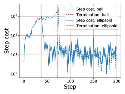
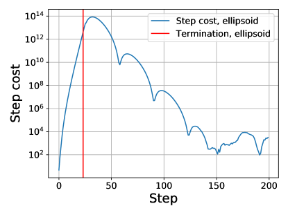
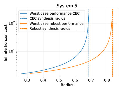
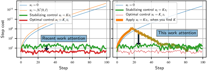
In this work, we address the problem of finding a stabilizing controller for a linear dynamical system in a single online trajectory. On the left plot of Figure 1, we show the difference in cost between finding a stabilizing controller and an optimal one. When the true system is unstable, and no knowledge of a stabilizing controller is available, the system costs grow exponentially fast.

Contributions

We extend the robust formulation of Dean et al. (2019) from stabilizing all systems within some spectral norm around estimates, to the more general case when the synthesized controller stabilizes all systems within an ellipsoidal uncertainty set. We extend the obtained result to our main contribution where we prove equivalence between common robust controller synthesis algorithms. In particular we show that the controller synthesis of Umenberger et al. (2019), which also tries to stabilize systems inside ellipsoid around estimates, and the derived SLS synthesis for ellipsoids share the same feasibility region: when one algorithm finds a stabilizing controller, so does the other one. Using the proposed robust controller syntheses applied to the ellipsoidal regions obtained from the Bayesian setting we propose an algorithm eXploration. The vanilla version synthesizes a stabilizing controller for the true underlying system in finite time with high probability. The vanilla eXploration approach probes the unknown system with zero-mean Gaussian actions. Additionally, we empirically show that with the robustly motivated choices of system probing which are different from zero-mean Gaussian, we reduce the length of the eXploration and substantially lower the total suffered cost. We demonstrate the practicality of our method on the standard common benchmark problems.
Refer to caption
Figure 1: While recent work attention was mostly focused on how to adaptively progress from a given stabilizing controller to an optimal one, this work attention is how to find a stabilizing controller in the single-trajectory setting.

1.1 Related Work

Linear dynamical systems have been extensively studied in control theory (cf., Zhou et al. (1996)), nevertheless the interest reemerged in the Machine Learning community after the seminal work of Abbasi-Yadkori and Szepesvári (2011). Cohen et al. (2019); Mania et al. (2019); Simchowitz and Foster (2020); Abeille and Lazaric (2020); Lale et al. (2020); Faradonbeh et al. (2020) and many others show that approaches relying on the optimism in the face of uncertainty (OFU) principle or certainty equivalence principle achieve 𝒪(T)𝒪𝑇\mathcal{O}(\sqrt{T}) regret in the online single trajectory setting with stochastic disturbances. However, most of the algorithms in this setting require the knowledge of an initial stabilizing controller, which might not always be available.

System Identification

The first step in eXploration is to learn the true system matrices A,Bsubscript𝐴subscript𝐵A_{*},B_{*} using System Identification tools. Simchowitz et al. (2018) show that the ordinary least squares (OLS) estimator attains a near optimal error rate 𝒪(1/i)𝒪1𝑖\mathcal{O}(1/\sqrt{i}), where i𝑖i is the number of steps in the single trajectory setting for the case when ρ(A)1𝜌subscript𝐴1\rho(A_{*})\leq 1111Spectral radius of matrix A𝐴A is defined as ρ(A)=max{|λ||v:Av=λv}𝜌𝐴:conditional𝜆𝑣𝐴𝑣𝜆𝑣\rho(A)=\max\{\left\lvert\lambda\right\rvert|\exists v:Av=\lambda v\}. They further argue that more unstable systems are easier to estimate and prove exponential error decay for one dimensional unstable systems. Faradonbeh et al. (2018a) tackle more challenging general systems with eigenvalues everywhere but on the unit circle. They show that in this case for regular222System is regular if every eigenvalue μ𝜇\mu of Asubscript𝐴A_{*} with |μ|>1𝜇1\left\lvert\mu\right\rvert>1, has geometric multiplicity equal to 1. systems the ordinary least squares (OLS) estimator is consistent. Further, Sarkar and Rakhlin (2019) extend the OLS consistency to general regular systems. They show that the estimation error scales as 𝒪(1/i)𝒪1𝑖\mathcal{O}(1/\sqrt{i}). Umenberger et al. (2019) show that the OLS is the same as the maximum (Gaussian) likelihood estimator. They further introduce an ellipsoid region around the estimates where the system lies with high confidence. We extend their idea to the Bayesian setting, where we assume a Gaussian prior on the system parameters, and show that, in this case, the maximum a-posteriori estimator is equivalent to the regularized least squares (RLS) estimator. Applying the analysis of Sarkar and Rakhlin (2019) we show that the associated data dependent high probability credibility regions are consistent.

Controller Synthesis

The second step in eXploration is to synthesize a stabilizing controller for all systems in the credibility region that the System Identification step outputs. Dean et al. (2019) derive a robust semi-definite program based on system level synthesis (SLS) whose solution results in a stabilizing controller. They use a multi-trajectory setting to build 2-ball confidence regions around the estimates. We extend their algorithm to a tighter ellipsoidal region around the estimates. It turns out that the SLS synthesis with an ellipsoidal region finds a stabilizing controller as the robust LQR synthesis proposed by Umenberger et al. (2019). Faradonbeh et al. (2018b) propose a non-robust strategy and rely on well-known stability bounds of LQRs (Safonov and Athans, 1977). The main contribution is that they identify the system in closed-loop by sampling different controllers from a Gaussian distribution so that they avoid irregularity of the closed loop matrix a.s. The main practical limitation is that one needs to specify the running time of the algorithm a-priori using unknown system parameters. On the other hand eXploration provably terminates in finite time solving a convex SDP without specifying an a-priori termination time.

2 Problem Statement and Background

We consider a system evolving with the following linear dynamics

xi+1=Axi+Bui+wi+1,x0=0,formulae-sequencesubscript𝑥𝑖1subscript𝐴subscript𝑥𝑖subscript𝐵subscript𝑢𝑖subscript𝑤𝑖1subscript𝑥00\displaystyle x_{i+1}=A_{*}x_{i}+B_{*}u_{i}+w_{i+1},\quad x_{0}=0, (1)

where xidxsubscript𝑥𝑖superscriptsubscript𝑑𝑥x_{i}\in\mathbb{R}^{d_{x}} are states, uidusubscript𝑢𝑖superscriptsubscript𝑑𝑢u_{i}\in\mathbb{R}^{d_{u}} actions and (wi)i1i.i.d.𝒩(0,σw2I)(w_{i})_{i\geq 1}\stackrel{{\scriptstyle\mathclap{i.i.d.}}}{{\sim}}\mathcal{N}(0,\sigma_{w}^{2}I) unobserved Gaussian noise in dxsuperscriptsubscript𝑑𝑥\mathbb{R}^{d_{x}}. The matrices Adx×dx,Bdx×duformulae-sequencesubscript𝐴superscriptsubscript𝑑𝑥subscript𝑑𝑥subscript𝐵superscriptsubscript𝑑𝑥subscript𝑑𝑢A_{*}\in\mathbb{R}^{d_{x}\times d_{x}},B_{*}\in\mathbb{R}^{d_{x}\times d_{u}} are unknown transition matrices. We sample actions uisubscript𝑢𝑖u_{i} from a policy π𝜋\pi, which at every step i𝑖i maps the current history ((xj)ji,(uj)j<i)subscriptsubscript𝑥𝑗𝑗𝑖subscriptsubscript𝑢𝑗𝑗𝑖((x_{j})_{j\leq i},(u_{j})_{j<i}) to a distribution over actions. We assume that the system is stabilizable, which means that there exists a matrix Kdu×dx𝐾superscriptsubscript𝑑𝑢subscript𝑑𝑥K\in\mathbb{R}^{d_{u}\times d_{x}} such that ρ(A+BK)<1𝜌subscript𝐴subscript𝐵𝐾1\rho(A_{*}+B_{*}K)<1. At step i𝑖i, we incur a cost cisubscript𝑐𝑖c_{i} given by

ci=xiQxi+uiRui,subscript𝑐𝑖superscriptsubscript𝑥𝑖top𝑄subscript𝑥𝑖superscriptsubscript𝑢𝑖top𝑅subscript𝑢𝑖\displaystyle c_{i}=x_{i}^{\top}Qx_{i}+u_{i}^{\top}Ru_{i}, (2)

where Qdx×dx,Rdu×duformulae-sequence𝑄superscriptsubscript𝑑𝑥subscript𝑑𝑥𝑅superscriptsubscript𝑑𝑢subscript𝑑𝑢Q\in\mathbb{R}^{d_{x}\times d_{x}},R\in\mathbb{R}^{d_{u}\times d_{u}} are known positive definite matrices.

When the system matrices A,Bsubscript𝐴subscript𝐵A_{*},B_{*} are known, the optimal solution in the infinite horizon setting is given by the fixed map ui=Kxisubscript𝑢𝑖subscript𝐾subscript𝑥𝑖u_{i}=K_{*}x_{i} and the optimal cost is Jsubscript𝐽J_{*} (Bertsekas, 2000). Hereby, K=(R+BPB)1BPAsubscript𝐾superscript𝑅superscriptsubscript𝐵top𝑃subscript𝐵1superscriptsubscript𝐵top𝑃subscript𝐴K_{*}=-(R+B_{*}^{\top}PB_{*})^{-1}B_{*}^{\top}PA_{*}, where P𝑃P is the solution to the discrete algebraic Ricatti equation of the system, P=DARE(A,B,Q,R)𝑃𝐷𝐴𝑅𝐸subscript𝐴subscript𝐵𝑄𝑅P=DARE(A_{*},B_{*},Q,R).

While most of the recent work focuses on finding the optimal controller Ksubscript𝐾K_{*} suffering the least possible cummulative cost, they require the knowledge of an initial stabilizing controller K0subscript𝐾0K_{0}. In this work, we focus on finding a stabilizing controller in the single-trajectory setting. If the system is unstable, the difference between using a stabilizing controller or not using a stabilizing controller results in an exponential difference in the suffered cost due to blow-up of the system. On the other hand, the difference between using a stabilizing controller and the optimal one results in a linear difference in the suffered cost as summarized in Figure 1. Consequently, it is very desirable that a stabilizing controller is found quickly.

3 Identifying A Stabilizing Controller

As we are trying to stabilize the system without knowing anything non-trivial about the dynamical system certain blow-up of the state from zero is inevitable. As this blow-up increases exponentially fast the state magnitude, it is essential that this period is kept very short. There are conceptually two variables we can influence as algorithm designers, a) what control signal we input to the system what we refer to as probing and b) stopping rule, which determines when we should stop probing and sufficient information about the system has been gathered to construct a stabilizing controller.

In this work we focus on the latter and derive a data-dependent stopping rule based on feasibility of a semi-definite program. Our method is versatile and can be combined with any control inputs and we show that it terminates in finite time under zero-mean Gaussian control inputs. Our formalism is derived under a general assumption that we can construct estimates of the system matrices and ellipsoidal sets which with high probability contain the true system matrices or they serve as a surrogate for this task as is the case with the Bayesian approach. More specifically, we derive our results under the assumption that after playing a policy π𝜋\pi for i𝑖i steps we have estimates (A^i,B^i)subscript^𝐴𝑖subscript^𝐵𝑖(\widehat{A}_{i},\widehat{B}_{i}) of the system (A,B)subscript𝐴subscript𝐵(A_{*},B_{*}) and ellipsoid

Θi={(A,B)|ΔDiΔI,Δ=(A,B)(A^i,B^i)}subscriptΘ𝑖conditional-set𝐴𝐵formulae-sequenceprecedes-or-equalssuperscriptΔtopsubscript𝐷𝑖Δ𝐼superscriptΔtop𝐴𝐵subscript^𝐴𝑖subscript^𝐵𝑖\Theta_{i}=\{(A,B)|\Delta^{\top}D_{i}\Delta\preceq I,\Delta^{\top}=(A,B)-(\widehat{A}_{i},\widehat{B}_{i})\} (3)

around estimates for which we believe that (A,B)Θisubscript𝐴subscript𝐵subscriptΘ𝑖(A_{*},B_{*})\in\Theta_{i}. Here Disubscript𝐷𝑖D_{i} is a data-dependent positive definite matrix. We present an example of how to construct such ellipsoidal region in Section 3.4.

In the following two subsections, we derive two different robust synthesis algorithms for uncertainty sets in the ellipsoidal region (3). In Section 3.3, prove that these two seemingly different approaches are actually equivalent in terms of robust stability.

3.1 Robust System Level Synthesis (SLS)

Our first stopping rule is based on a relaxation stemming from the SLS framework (Wang et al., 2019). In particular, we extend the work of Dean et al. (2019) to ellipsoidal regions (3). Dean et al. (2019) show that a controller K𝐾K stabilizes all systems (A,B)Θi𝐴𝐵subscriptΘ𝑖(A,B)\in\Theta_{i} if for every (AB)Θi𝐴𝐵subscriptΘ𝑖(A~{}B)\in\Theta_{i} we have:

Δ(IK)(zIA^iB^iK)1<1,subscriptdelimited-∥∥superscriptΔtopmatrix𝐼𝐾superscript𝑧𝐼subscript^𝐴𝑖subscript^𝐵𝑖𝐾1subscript1\displaystyle\left\lVert\Delta^{\top}\begin{pmatrix}I\\ K\end{pmatrix}\left(zI-\widehat{A}_{i}-\widehat{B}_{i}K\right)^{-1}\right\rVert_{\mathcal{H}_{\infty}}<1, (4)

where Δ=(AB)(A^iB^i)superscriptΔtop𝐴𝐵subscript^𝐴𝑖subscript^𝐵𝑖\Delta^{\top}=(A~{}B)-(\widehat{A}_{i}~{}\widehat{B}_{i}).The subscript\mathcal{H}_{\infty}-norm for a function f:d×d:𝑓superscript𝑑𝑑f:\mathbb{C}\to\mathbb{C}^{d\times d} is defined as f=supz𝔻f(z)subscriptdelimited-∥∥𝑓subscriptsubscriptsupremum𝑧𝔻delimited-∥∥𝑓𝑧\left\lVert f\right\rVert_{\mathcal{H}_{\infty}}=\sup_{z\in\partial\mathbb{D}}\left\lVert f(z)\right\rVert, where 𝔻={z|z<1}𝔻conditional-set𝑧delimited-∥∥𝑧1\mathbb{D}=\{z\in\mathbb{C}|\left\lVert z\right\rVert<1\} is a unit disk in the complex plane. With the current formulation we need to ensure that subscript\mathcal{H}_{\infty}-norm constraint (4) holds for every (A,B)Θi𝐴𝐵subscriptΘ𝑖(A,B)\in\Theta_{i}. The main difference with Dean et al. (2019) is that we apply the S-Lemma of Luo et al. (2004) to obtain an equivalent formulation with a single subscript\mathcal{H}_{\infty}-norm constraint using the ellipsoidal region instead of a 2-ball. Next, we transform the subscript\mathcal{H}_{\infty}-norm constraint to a convex semi-definite constraint applying the KYP-Lemma (Bart et al., 2018). The equivalent feasibility problem reads:

minX0,S,t(0,1)0,subscriptformulae-sequencesucceeds𝑋0𝑆𝑡010\displaystyle\min_{X\succ 0,S,t\in(0,1)}0, s.t.(XIA^iX+B^iS0(A^iX+B^iS)X(XS)0(XS)tD)0.succeeds-or-equalss.t.matrix𝑋𝐼subscript^𝐴𝑖𝑋subscript^𝐵𝑖𝑆0superscriptsubscript^𝐴𝑖𝑋subscript^𝐵𝑖𝑆top𝑋superscriptmatrix𝑋𝑆top0matrix𝑋𝑆𝑡𝐷0\displaystyle\qquad\text{s.t.}\quad\begin{pmatrix}X-I&\widehat{A}_{i}X+\widehat{B}_{i}S&0\\ (\widehat{A}_{i}X+\widehat{B}_{i}S)^{\top}&X&\begin{pmatrix}X\\ S\end{pmatrix}^{\top}\\ 0&\begin{pmatrix}X\\ S\end{pmatrix}&tD\\ \end{pmatrix}\succeq 0. (5)

The stabilizing controller is extracted from the solution of the Robust SLS (5) as K=SX1𝐾𝑆superscript𝑋1K=SX^{-1}. We show the derivation details in the Appendix B.

3.2 Robust Linear Quadratic Regulator (LQR)

The derivation of our second robust controller synthesis is based on the reformulation of the LQR problem, which finds the optimal infinite horizon controller. This reformulations lends itself to an efficient SDP relaxation (Boyd et al., 1994). We follow the exposition from Cohen et al. (2018), assuming we know matrices A,Bsubscript𝐴subscript𝐵A_{*},B_{*} we can obtain the optimal infinite controller Ksubscript𝐾K_{*} by first solving

minΣ0subscriptsucceeds-or-equalsΣ0\displaystyle\min_{\Sigma\succeq 0} Tr((Q00R)Σ)Trmatrix𝑄00𝑅Σ\displaystyle\operatorname{Tr}\left(\begin{pmatrix}Q&0\\ 0&R\end{pmatrix}\Sigma\right) (6)
s.t.Σxx(AB)Σ(AB)+σw2I,succeeds-or-equalss.t.subscriptΣ𝑥𝑥subscript𝐴subscript𝐵Σsuperscriptsubscript𝐴subscript𝐵topsuperscriptsubscript𝜎𝑤2𝐼\displaystyle\text{s.t.}\quad\Sigma_{xx}\succeq(A_{*}~{}B_{*})\Sigma(A_{*}~{}B_{*})^{\top}+\sigma_{w}^{2}I,

and then extracting the optimal controller as K=ΣuxΣxx1subscript𝐾subscriptΣ𝑢𝑥superscriptsubscriptΣ𝑥𝑥1K_{*}=\Sigma_{ux}\Sigma_{xx}^{-1}. Here Σ=(ΣxxΣxuΣuxΣuu)ΣmatrixsubscriptΣ𝑥𝑥subscriptΣ𝑥𝑢subscriptΣ𝑢𝑥subscriptΣ𝑢𝑢\Sigma=\begin{pmatrix}\Sigma_{xx}&\Sigma_{xu}\\ \Sigma_{ux}&\Sigma_{uu}\end{pmatrix}, where Σxxdx×dxsubscriptΣ𝑥𝑥superscriptsubscript𝑑𝑥subscript𝑑𝑥\Sigma_{xx}\in\mathbb{R}^{d_{x}\times d_{x}} and Σuudu×dusubscriptΣ𝑢𝑢superscriptsubscript𝑑𝑢subscript𝑑𝑢\Sigma_{uu}\in\mathbb{R}^{d_{u}\times d_{u}}, represents the joint covariance matrix of the state and action. The derivation with the motivation behind the SDP (6) is given in Appendix C, where we also show in Lemma C.3 that the semi-definite constraint in the SDP (6) ensures that controller synthesized as K=ΣuxΣxx1𝐾subscriptΣ𝑢𝑥superscriptsubscriptΣ𝑥𝑥1K=\Sigma_{ux}\Sigma_{xx}^{-1} stabilize the system A,Bsubscript𝐴subscript𝐵A_{*},B_{*}. Inspired by Umenberger et al. (2019), the robust formulation of the SDP problem (6) is:

minΣ0subscriptsucceeds-or-equalsΣ0\displaystyle\min_{\Sigma\succeq 0} Tr((Q00R)Σ)Trmatrix𝑄00𝑅Σ\displaystyle\operatorname{Tr}\left(\begin{pmatrix}Q&0\\ 0&R\end{pmatrix}\Sigma\right) (7)
s.t. (A,B)Θi:Σxx(AB)Σ(AB)+σw2I.:s.t. for-all𝐴𝐵subscriptΘ𝑖succeeds-or-equalssubscriptΣ𝑥𝑥𝐴𝐵Σsuperscript𝐴𝐵topsuperscriptsubscript𝜎𝑤2𝐼\displaystyle\text{s.t. }\forall(A,B)\in\Theta_{i}:~{}\Sigma_{xx}\succeq(A~{}B)\Sigma(A~{}B)^{\top}+\sigma_{w}^{2}I.

As in Section 3.1 we have to ensure that one condition has to hold for every system in the ellipsoid ΘisubscriptΘ𝑖\Theta_{i}. Applying the S-Lemma we reformulate problem given by eq. 7 to an equivalent convex SDP:

minΣ0,t0subscriptformulae-sequencesucceeds-or-equalsΣ0𝑡0\displaystyle\min_{\Sigma\succeq 0,t\geq 0} Tr((Q00R)Σ)Trmatrix𝑄00𝑅Σ\displaystyle\operatorname{Tr}\left(\begin{pmatrix}Q&0\\ 0&R\end{pmatrix}\Sigma\right) (8)
s.t. (Σxx(A^iB^i)Σ(A^iB^i)(t+σw2)I(A^iB^i)ΣΣ(A^iB^i)tDΣ)0.succeeds-or-equalss.t. matrixsubscriptΣ𝑥𝑥subscript^𝐴𝑖subscript^𝐵𝑖Σsuperscriptsubscript^𝐴𝑖subscript^𝐵𝑖top𝑡superscriptsubscript𝜎𝑤2𝐼subscript^𝐴𝑖subscript^𝐵𝑖ΣΣsuperscriptsubscript^𝐴𝑖subscript^𝐵𝑖top𝑡𝐷Σ0\displaystyle\text{s.t. }\begin{pmatrix}\Sigma_{xx}-(\widehat{A}_{i}~{}\widehat{B}_{i})\Sigma(\widehat{A}_{i}~{}\widehat{B}_{i})^{\top}-(t+\sigma_{w}^{2})I&(\widehat{A}_{i}~{}\widehat{B}_{i})\Sigma\\ \Sigma(\widehat{A}_{i}~{}\widehat{B}_{i})^{\top}&tD-\Sigma\end{pmatrix}\succeq 0.

The stabilizing controller is extracted from the optimal solution as K=ΣuxΣxx1𝐾subscriptΣ𝑢𝑥superscriptsubscriptΣ𝑥𝑥1K=\Sigma_{ux}\Sigma_{xx}^{-1}.

3.3 Equivalence

At first glance one could think that we have derived two completely different control synthesis procedures, however as we will see this is not the case and the two optimization problems have the same feasible regions.

Theorem 3.1.

The Robust SLS given by Equation 5 has a nonempty solution if and only if the Robust LQR given by Equation 8 has a nonempty solution.

The proof of the theorem is provided in Appendix D. Despite the fact that the two SDPs (5) and (8) have the same feasible solutions, they differ in the objective. The robust SLS (5) is maximizing a constant for which we can find a stabilizing controller, whereas the Robust LQR (8) is minimizing the upper bound of the maximal infinite horizon cost of the systems in ΘisubscriptΘ𝑖\Theta_{i}. The specific nature of the objective is not interesting for the stopping rule, however can have practically dramatic impact in downstream tasks. For different possible objective for the SLS synthesis (5) please refer to Section 4.1.

3.4 Example: Bayesian credible sets

In this section, we show a particular design choice of estimators A^i,B^isubscript^𝐴𝑖subscript^𝐵𝑖\widehat{A}_{i},\widehat{B}_{i} and region ΘisubscriptΘ𝑖\Theta_{i} which results from the Bayesian setting. Inspired by the work of Umenberger et al. (2019), we place a Gaussian prior333Regarding the sense of this assumption and cases when this assumption fails look at Section 5.1 on the system matrices A,Bsubscript𝐴subscript𝐵A_{*},B_{*} i.e. vec(A,B)𝒩(0,σw2/λI)similar-tovecsubscript𝐴subscript𝐵𝒩0superscriptsubscript𝜎𝑤2𝜆𝐼\operatorname*{vec}(A_{*},B_{*})\sim\mathcal{N}\left(0,\sigma_{w}^{2}/\lambda I\right). In this case we have explicit formulas for the posterior distribution of vec(A,B)|(xj)ji,(uj)j<iconditionalvecsubscript𝐴subscript𝐵subscriptsubscript𝑥𝑗𝑗𝑖subscriptsubscript𝑢𝑗𝑗𝑖\operatorname*{vec}(A_{*},B_{*})|(x_{j})_{j\leq i},(u_{j})_{j<i}. As derived in the Appendix A it turns out the posterior is also Gaussian and the MAP estimator vec(A^i,B^i)vecsubscript^𝐴𝑖subscript^𝐵𝑖\operatorname*{vec}(\widehat{A}_{i},\widehat{B}_{i}) is exactly the RLS estimator:

A^i,B^i=argminA,Bj=0i1xj+1AxjBuj22+λ(AB)F2.subscript^𝐴𝑖subscript^𝐵𝑖subscriptargmin𝐴𝐵superscriptsubscript𝑗0𝑖1superscriptsubscriptdelimited-∥∥subscript𝑥𝑗1𝐴subscript𝑥𝑗𝐵subscript𝑢𝑗22𝜆superscriptsubscriptdelimited-∥∥𝐴𝐵𝐹2\displaystyle\widehat{A}_{i},\widehat{B}_{i}=\operatorname*{argmin}_{A,B}\sum_{j=0}^{i-1}\left\lVert x_{j+1}-Ax_{j}-Bu_{j}\right\rVert_{2}^{2}+\lambda\left\lVert(A~{}B)\right\rVert_{F}^{2}. (9)

Moreover, the Bayesian credibility region is Θi={(AB)|ΔDiΔI,Δ=(AB)(A^i,B^i)}subscriptΘ𝑖conditional-set𝐴𝐵formulae-sequenceprecedes-or-equalssuperscriptΔtopsubscript𝐷𝑖Δ𝐼superscriptΔtop𝐴𝐵subscript^𝐴𝑖subscript^𝐵𝑖\Theta_{i}=\{(A~{}B)|\Delta^{\top}D_{i}\Delta\preceq I,\Delta^{\top}=(A~{}B)-(\widehat{A}_{i},\widehat{B}_{i})\}. Here Disubscript𝐷𝑖D_{i} represents the scaled inverse covariance matrix of the posterior distribution and is explicitly given as Di=1cδσw2(j=1izjzj+λI)subscript𝐷𝑖1subscript𝑐𝛿superscriptsubscript𝜎𝑤2superscriptsubscript𝑗1𝑖subscript𝑧𝑗superscriptsubscript𝑧𝑗top𝜆𝐼D_{i}=\frac{1}{c_{\delta}\sigma_{w}^{2}}\left(\sum_{j=1}^{i}z_{j}z_{j}^{\top}+\lambda I\right), where zj=(xjuj)superscriptsubscript𝑧𝑗topsuperscriptsubscript𝑥𝑗topsuperscriptsubscript𝑢𝑗topz_{j}^{\top}=(x_{j}^{\top}u_{j}^{\top}) and cδsubscript𝑐𝛿c_{\delta} is the (1δ)1𝛿(1-\delta)-quantile of the χ2superscript𝜒2\chi^{2} distribution with dx(dx+du)subscript𝑑𝑥subscript𝑑𝑥subscript𝑑𝑢d_{x}(d_{x}+d_{u}) degrees of freedom. With this definition of ΘisubscriptΘ𝑖\Theta_{i} we have (AB)Θisubscript𝐴subscript𝐵subscriptΘ𝑖(A_{*}~{}B_{*})\in\Theta_{i} w.p. 1δ1𝛿1-\delta.

4 eXploration Algorithm

We now show how to use the derived results (c.f., Section 3) to provably find a robust controller in the Bayesian setting. In the Appendix E we show how to initialize the algorithms, specifically OSLO (Cohen et al., 2019) and CEC (Simchowitz and Foster, 2020), which need a stabilizing controller as an input, with the proposed eXploration algorithm.

Algorithm 1 eXploration
  Input: x0=0,λ,δsubscript𝑥00𝜆𝛿x_{0}=0,\lambda,\delta
  for i=1,𝑖1i=1,\ldots do
     \colorblue /* Probing Signal /*
     Play uiπ(|x1:i,u1:i1)u_{i}\sim\pi(\cdot|x_{1:i},u_{1:i-1}) and observe state xi+1subscript𝑥𝑖1x_{i+1}.
     \colorblue /* Stopping Rule /*
     Build a confidence region ΘisubscriptΘ𝑖\Theta_{i}, such that (AB)Θisubscript𝐴subscript𝐵subscriptΘ𝑖(A_{*}~{}B_{*})\in\Theta_{i} w.p. 1δ1𝛿1-\delta. (c.f. Section 3.4)
     Solve a robust controller synthesis (A,B)Θifor-all𝐴𝐵subscriptΘ𝑖\forall(A,B)\in\Theta_{i}. (c.f. Section 3.1 or Section 3.2)
     if a controller is found return stabilizing controller K0subscript𝐾0K_{0}
  end for

The learner explores using a policy π𝜋\pi that only depends on the past states and inputs. Using the collected data, it builds an empirical estimate and a confidence region around it. Finally, it attempts to solve a robust controller synthesis problem. If it fails, the algorithm continues. If it succeeds, the algorithm terminates and returns a provably stabilizing controller for the true underlying system.

The credibility regions must contain the true system with probability 1δ1𝛿1-\delta only at the time isuperscript𝑖i^{*} in which a controller is found and not uniformly over all time steps. This is crucial as it allows us to use tight credibility regions. Then, with probability δ𝛿\delta, the algorithm might fail to return a stabilizing controller, and it will return a stabilizing controller with probability 1δ1𝛿1-\delta.

In this section, we analyze the Vanilla eXploration variant, in which the policy is to choose independent zero-mean Gaussian action, i.e., uiπ(|x1:i,u1:i1)=𝒩(0,σu2I)u_{i}\sim\pi(\cdot|x_{1:i},u_{1:i-1})=\mathcal{N}(0,\sigma_{u}^{2}I). Next, we prove that Vanilla eXploration finishes in O~(1)~𝑂1\widetilde{O}(1) time. In Section 4.1, we discuss different probing heuristics that perform well in practice but where we lose the finte time termination guarantee. Nevertheless, the algorithm still remains valid: if it terminates, the resulting controller provably stabilizes the system.

Theorem 4.1.

Assuming the aforementioned setting, then with probability 1δ1𝛿1-\delta Vanilla eXploration returns a stabilizing controller for (A,B)subscript𝐴subscript𝐵(A_{*},B_{*}) in time:

𝒪~(polylog(δ)(1+K2)2(zIABK)12),~𝒪polylog𝛿superscript1subscriptnorm𝐾22superscriptsubscriptdelimited-∥∥superscript𝑧𝐼subscript𝐴subscript𝐵𝐾1subscript2\displaystyle\widetilde{\mathcal{O}}\left(\operatorname{polylog}(\delta)(1+\|K\|_{2})^{2}\left\lVert(zI-A_{*}-B_{*}K)^{-1}\right\rVert_{\mathcal{H}_{\infty}}^{2}\right), (10)

where K𝐾K is any stabilizing static controller.

Proof Sketch:

First, note that since we assume that entries of A,Bsubscript𝐴subscript𝐵A_{*},B_{*} are sampled from independent Gaussian, system (A,B)subscript𝐴subscript𝐵(A_{*},B_{*}) is stabilizable a.s. If K𝐾K is a stabilizing controller we derive in the Appendix F, extending the results of Dean et al. (2019), that the SLS synthesis (5) is feasible if

𝒪((1+K2)2(zIABK)12)λmin(D).𝒪superscript1subscriptdelimited-∥∥𝐾22superscriptsubscriptdelimited-∥∥superscript𝑧𝐼subscript𝐴subscript𝐵𝐾1subscript2subscript𝜆𝑚𝑖𝑛𝐷\displaystyle\mathcal{O}\left((1+\left\lVert K\right\rVert_{2})^{2}\left\lVert(zI-A_{*}-B_{*}K)^{-1}\right\rVert_{\mathcal{H}_{\infty}}^{2}\right)\leq\lambda_{min}(D). (11)

To obtain the best bound we choose a stabilizing controller K𝐾K such that the left hand side of Equation 11 is minimized. From Equation 11 follows that as soon as the smallest eigenvalue of the matrix D𝐷D is large enough, the robust synthesis will be feasible. At the same time from the analysis of Sarkar and Rakhlin (2019) follows that Ω~(i)IDiprecedes-or-equals~Ω𝑖𝐼subscript𝐷𝑖\widetilde{\Omega}(i)I\preceq D_{i} for every regular system. Again, since we assume a Gaussian prior on (A,B)subscript𝐴subscript𝐵(A_{*},B_{*}), the system is regular a.s. Assembling the pieces together we arrive at the result, for which we provide more detailed proof in the Appendix F.

4.1 Different probing signals with eXploration

The VANILLA eXploration approach takes random actions ui𝒩(0,σu2I)similar-tosubscript𝑢𝑖𝒩0superscriptsubscript𝜎𝑢2𝐼u_{i}\sim\mathcal{N}(0,\sigma_{u}^{2}I). For such a choice we can guarantee that Algorithm 1 terminates after constant time, depending only on the system parameters. However, as we demonstrate in our experiments (c.f., Appendix H of the extended paper (Treven et al., 2020)), the states grow exponentially during this phase, which can be highly problematic for certain applications. We now propose improved, data-dependent policies to counteract this blow-up. In particular, we consider playing ui𝒩(Kixi,σu2I)similar-tosubscript𝑢𝑖𝒩subscript𝐾𝑖subscript𝑥𝑖superscriptsubscript𝜎𝑢2𝐼u_{i}\sim\mathcal{N}(K_{i}x_{i},\sigma_{u}^{2}I), where Kisubscript𝐾𝑖K_{i} is a controller picked at time i𝑖i. With such a controller, we generally lose the theoretical guarantee that the Algorithm 1 will terminate. However, the data dependent credibility region on estimation errors from section 3.4 (and thus the validity of the stopping condition) is still valid and we can run Algorithm 1. With data dependent inputs, we cannot guarantee that the minimum eigenvalue of Disubscript𝐷𝑖D_{i} grows as Ω~(i)~Ω𝑖\tilde{\Omega}(i). Next, we discuss different choices for controller Kisubscript𝐾𝑖K_{i} that we study in our experiments.

CEC

As first possibility, we could act as if the estimators A^i,B^isubscript^𝐴𝑖subscript^𝐵𝑖\widehat{A}_{i},\widehat{B}_{i} are the true system matrices and we compute the controller Kisubscript𝐾𝑖K_{i} as the optimal controller:

Ki=(R+B^iPB^i)1B^iPA^i,subscript𝐾𝑖superscript𝑅superscriptsubscript^𝐵𝑖top𝑃subscript^𝐵𝑖1superscriptsubscript^𝐵𝑖top𝑃subscript^𝐴𝑖K_{i}=-(R+\widehat{B}_{i}^{\top}P\widehat{B}_{i})^{-1}\widehat{B}_{i}^{\top}P\widehat{A}_{i}, (12)

where Pi=DARE(A^i,B^i,Q,R)subscript𝑃𝑖DAREsubscript^𝐴𝑖subscript^𝐵𝑖𝑄𝑅P_{i}=\operatorname{DARE}(\widehat{A}_{i},\widehat{B}_{i},Q,R), i.e., we act using Certainty Equivalent Control (CEC).

MinMax

For the second Kisubscript𝐾𝑖K_{i} we consider controller which minimizes the maximal closed loop norm of the systems in ΘisubscriptΘ𝑖\Theta_{i}. At every time step we synthesize the controller Kisubscript𝐾𝑖K_{i} as

Ki=argminKmax(A,B)ΘiA+BK2\displaystyle K_{i}=\operatorname*{argmin}_{K}\max_{(A,B)\in\Theta_{i}}\left\lVert A+BK\right\rVert_{2} (13)

The controller defined in Equation 13 can be efficiently computed via a convex SDP. We derive the convex SDP formulation of the min max problem given by Equation 13 in Appendix G of the extended paper (Treven et al., 2020).

RelaxedSLS

As a third alternative we relax the constraint t(0,1)𝑡01t\in(0,1) to t0𝑡0t\geq 0 in the SDP feasibility problem (5), and minimize the value of t𝑡t, i.e.:

minX0,S,t0tsubscriptformulae-sequencesucceeds𝑋0𝑆𝑡0𝑡\displaystyle\min_{X\succ 0,S,t\geq 0}t    s.t. semi-definite constraint (5) (14)

The controller is then synthesized as Ki=SX1subscript𝐾𝑖𝑆superscript𝑋1K_{i}=SX^{-1}. With such relaxation, the SDP is always feasible. The interpretation of this relaxation is that when t1𝑡1t\geq 1 we find a controller that stabilizes all systems (A,B)𝐴𝐵(A,B) in a smaller confidence region around the estimates (A^i,B^i)subscript^𝐴𝑖subscript^𝐵𝑖(\widehat{A}_{i},\widehat{B}_{i}). Furthermore, this algorithms returns a provably stabilizing controller when t<1𝑡1t<1. Although in principle we could also increase Disubscript𝐷𝑖D_{i} in the Robust LQR synthesis in (8), this requires a tedious exponential line search, whereas the RelaxedSLS synthesis does this automatically.

5 Experiments

In this section, we critically evaluate the different components of eXploration empirically. In Section 5.1, we investigate when the credibility regions are correct and when do they fail on a fixed system A,Bsubscript𝐴subscript𝐵A_{*},B_{*}. In particular, the algorithm fails when the prior parameter λ𝜆\lambda is too large. To overcome this issue, we suggest a way of selecting the prior parameter λ𝜆\lambda, given some mild privileged information. In Section 5.2, we compare the time it takes to find a stabilizing controller and the total cost suffered using different probing signals. Although Vanilla eXploration provably terminates, the heuristic variants perform better in practice. In all the considered examples the cost matrices Q𝑄Q and R𝑅R are equal to the identity matrix of the appropriate dimensions. The scales of unobserved and played noise covariance matrices are σw2=σu2=1superscriptsubscript𝜎𝑤2superscriptsubscript𝜎𝑢21\sigma_{w}^{2}=\sigma_{u}^{2}=1. We set the probability of failure to δ=0.1𝛿0.1\delta=0.1.

5.1 Data Dependent Credibility Region

To illustrate how eXploration builds the credibility regions, we consider a one dimensional system A=1.5,B=1.8formulae-sequencesubscript𝐴1.5subscript𝐵1.8A_{*}=1.5,B_{*}=1.8. We select λ=14𝜆14\lambda=\frac{1}{4} and λ=3𝜆3\lambda=3 and show consecutive credibility regions in Figure 2. As we can see, the credibility region ΘisubscriptΘ𝑖\Theta_{i} shrinks as we see more data. For both choices of λ𝜆\lambda, Robust SLS and Robust LQR become feasible after 4 iterations and the algorithm terminates. Crucially, when λ𝜆\lambda is too large (i.e. too small variance of the prior), it may happen that the true parameters A,Bsubscript𝐴subscript𝐵A_{*},B_{*} are not inside the credibility region as we can see on in the middle subfigure of Figure 2.

Refer to caption
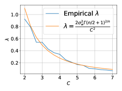
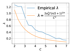
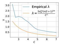
Figure 2: When credibility region ΘisubscriptΘ𝑖\Theta_{i} is small enough SDP (8) finds a controller which stabilizes every system in ΘisubscriptΘ𝑖\Theta_{i}. If we choose a Gaussian prior with too small covariance matrix the credibility regions ΘisubscriptΘ𝑖\Theta_{i} might not contain the true system and the resulting controller will not stabilize it. If we know a bound C𝐶C on the Frobenious norm of the system, experiments show that a reasonable choice for λ𝜆\lambda is λ1C2𝜆1superscript𝐶2\lambda\approx\frac{1}{C^{2}}.

This means that selecting λ𝜆\lambda is a problem-dependent quantity (as any prior). However, if we assume that we have of a constant C𝐶C such that (AB)FCsubscriptdelimited-∥∥subscript𝐴subscript𝐵𝐹𝐶\left\lVert(A_{*}~{}B_{*})\right\rVert_{F}\leq C, then in the Appendix I we suggest that selecting λ1/C2𝜆1superscript𝐶2\lambda\approx 1/C^{2}, results in the credibility regions which empirically contain the true system with probability at least 1δ1𝛿1-\delta. On the right most subfigure of Figure 2 we plot the largest λ𝜆\lambda for which we empirically observe that the one dimensional systems with (AB)Cdelimited-∥∥subscript𝐴subscript𝐵𝐶\left\lVert(A_{*}~{}B_{*})\right\rVert\leq C are inside regions ΘisubscriptΘ𝑖\Theta_{i} with empirical probability at least 1δ1𝛿1-\delta.

5.2 eXploration Performance

Next we will illustrate the cost suffered and time until we find a stabilizing controller on a system

A=(1.010.0100.011.010.0100.011.01),B=Iformulae-sequencesubscript𝐴matrix1.010.0100.011.010.0100.011.01subscript𝐵𝐼\displaystyle A_{*}=\begin{pmatrix}1.01&0.01&0\\ 0.01&1.01&0.01\\ 0&0.01&1.01\end{pmatrix},\quad B_{*}=I (15)

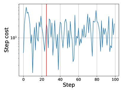
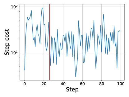
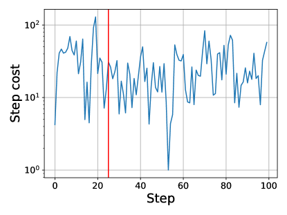
introduced by Dean et al. (2019), here we use λ=1𝜆1\lambda=1. We show a sample run with different heuristics in the Appendix H, here we show in Table 1 more in-depth analysis of the eXploration performances on system (15).

During exploration the agent suffers quadratic costs Equation 2 and at the eXploration termination leaves the system in state xTsubscript𝑥𝑇x_{T}. We define the total cost of exploration as

Cost=i=1T(xiQxi+uiRui)+xTPxT,Costsuperscriptsubscript𝑖1𝑇superscriptsubscript𝑥𝑖top𝑄subscript𝑥𝑖superscriptsubscript𝑢𝑖top𝑅subscript𝑢𝑖superscriptsubscript𝑥𝑇top𝑃subscript𝑥𝑇\text{Cost}=\sum_{i=1}^{T}\left(x_{i}^{\top}Qx_{i}+u_{i}^{\top}Ru_{i}\right)+x_{T}^{\top}Px_{T}, (16)

where P=DARE(A,B,Q,R)𝑃DAREsubscript𝐴subscript𝐵𝑄𝑅P=\operatorname{DARE}(A_{*},B_{*},Q,R), and T𝑇T is the termination time of eXploration. Since the cost can grow exponential with time we will report the logarithm of the Cost.

We compare robust synthesis with ellipsoidal bounds to two benchmarks. The first is robust synthesis with 2-ball estimation bounds of Dean et al. (2019). For the second benchmark we compare robust controller to the CEC which was used as a stabilizing controller in e.g. Faradonbeh et al. (2018b); Simchowitz and Foster (2020). In particular we analyze how large region around estimates they stabilize. For both controllers we use the tightest ellipsoidal bounds. To compute the stopping time when CEC stabilizes all systems inside the ellipsoidal bound we sample 1000 systems from the ellipsoid boundary and if CEC stabilizes all we stop eXploration444Note that it can still happen that CEC does not stabilize all systems inside ellipsoid, however already with this approximation robust controller stabilizes larger ellipsoidal region..

Using ellipsoidal compared to 2-ball bounds significantly reduces the number of steps of eXploration. Consequently we also suffer much less exploration cost. CEC naturally stabilizes some region around the estimates, however as we can see on the Table 1 CEC stabilizes smaller region compared to the robust controller, which is paramount in the case when the cost grows exponentially.

Table 1: Using ellipsoidal confidence regions significantly shortens the exploration time and consequently the cost. Robust controller stabilizes larger region than CEC which is crucial when the cost grows exponentially. We report median ±plus-or-minus\pm standard deviation.
Ellipsoidal region 2-ball region CEC as stopping time
Steps log(Cost)Cost\log(\text{Cost}) Steps log(Cost)Cost\log(\text{Cost}) Steps log(Cost)Cost\log(\text{Cost})
Vanilla 𝟒𝟒±8.2plus-or-minus448.2\mathbf{44\pm 8.2} 8.7±0.58plus-or-minus8.70.58\mathbf{8.7\pm 0.58} 84±18plus-or-minus841884\pm 18 11±1.1plus-or-minus111.111\pm 1.1 50±12plus-or-minus501250\pm 12 9.3±0.73plus-or-minus9.30.739.3\pm 0.73
CEC 𝟐𝟓±8.5plus-or-minus258.5\mathbf{25\pm 8.5} 6.2±1.1plus-or-minus6.21.1\mathbf{6.2\pm 1.1} 110±32plus-or-minus11032110\pm 32 7.4±0.62plus-or-minus7.40.627.4\pm 0.62 53±14plus-or-minus531453\pm 14 6.8±0.56plus-or-minus6.80.566.8\pm 0.56
MinMax 𝟐𝟒±𝟗plus-or-minus249\mathbf{24\pm 9} 7.1±3.2plus-or-minus7.13.2\mathbf{7.1\pm 3.2} 120±39plus-or-minus12039120\pm 39 7.9±3.1plus-or-minus7.93.17.9\pm 3.1 58±22plus-or-minus582258\pm 22 7.8±7.9plus-or-minus7.87.97.8\pm 7.9
RelaxedSLS 𝟐𝟔±8.9plus-or-minus268.9\mathbf{26\pm 8.9} 7.2±𝟑plus-or-minus7.23\mathbf{7.2\pm 3} 170±86plus-or-minus17086170\pm 86 9.1±2.9plus-or-minus9.12.99.1\pm 2.9 78±36plus-or-minus783678\pm 36 8.6±3.2plus-or-minus8.63.28.6\pm 3.2

6 Discussion and Conclusions

In Section 3 we presented two seemingly different relaxation techniques for solving Riccati equation under uncertainty. The two relaxations one in Z-transform space and the other convex relaxation in the SDP formulation lead to the same feasible regions. We instantiated our stopping rule with uncertainty regions over the system matrices constructed via Bayesian means, however the stopping rule is more general and can be used with confidence estimates constructed without prior assumptions assumption once we can guarantee uncertainty sets otherwise. To the best of our knowledge, provable anytime adaptive consistent confidence estimates for unstable linear systems are not known, but should these be constructable our stopping rule can be used with them.

References

  • Abbasi-Yadkori and Szepesvári (2011) Yasin Abbasi-Yadkori and Csaba Szepesvári. Regret bounds for the adaptive control of linear quadratic systems. volume 19 of Proceedings of Machine Learning Research, pages 1–26, Budapest, Hungary, 09–11 Jun 2011. JMLR Workshop and Conference Proceedings. URL http://proceedings.mlr.press/v19/abbasi-yadkori11a.html.
  • Abeille and Lazaric (2020) Marc Abeille and Alessandro Lazaric. Efficient optimistic exploration in linear-quadratic regulators via lagrangian relaxation. In Proceedings of Machine Learning and Systems 2020, pages 7388–7396. 2020.
  • ApS (2020) MOSEK ApS. MOSEK Optimizer API for Python 9.2.4, 2020. URL https://docs.mosek.com/9.2/pythonapi/index.html.
  • Bart et al. (2018) Harm Bart, Sanne ter Horst, André C.M. Ran, and Hugo J. Woerdeman, editors. Operator Theory, Analysis and the State Space Approach. Springer International Publishing, 2018. 10.1007/978-3-030-04269-1. URL https://doi.org/10.1007
  • Bertsekas (2000) Dimitri P. Bertsekas. Dynamic Programming and Optimal Control. Athena Scientific, 2nd edition, 2000. ISBN 1886529094.
  • Boyd et al. (1994) Stephen Boyd, Laurent El Ghaoui, Eric Feron, and Venkataramanan Balakrishnan. Linear matrix inequalities in system and control theory. SIAM, 1994.
  • Cohen et al. (2018) Alon Cohen, Avinatan Hasidim, Tomer Koren, Nevena Lazic, Yishay Mansour, and Kunal Talwar. Online linear quadratic control. volume 80 of Proceedings of Machine Learning Research, pages 1029--1038, Stockholmsmässan, Stockholm Sweden, 10--15 Jul 2018. PMLR. URL http://proceedings.mlr.press/v80/cohen18b.html.
  • Cohen et al. (2019) Alon Cohen, Tomer Koren, and Yishay Mansour. Learning linear-quadratic regulators efficiently with only T𝑇\sqrt{T} regret. In Kamalika Chaudhuri and Ruslan Salakhutdinov, editors, Proceedings of the 36th International Conference on Machine Learning, volume 97 of Proceedings of Machine Learning Research, pages 1300--1309, Long Beach, California, USA, 09--15 Jun 2019. PMLR. URL http://proceedings.mlr.press/v97/cohen19b.html.
  • Dean et al. (2019) Sarah Dean, Horia Mania, Nikolai Matni, Benjamin Recht, and Stephen Tu. On the sample complexity of the linear quadratic regulator. Foundations of Computational Mathematics, Aug 2019. ISSN 1615-3383. 10.1007/s10208-019-09426-y. URL https://doi.org/10.1007/s10208-019-09426-y.
  • Faradonbeh et al. (2018a) Mohamad Kazem Shirani Faradonbeh, Ambuj Tewari, and George Michailidis. Finite time identification in unstable linear systems. Automatica, 96:342--353, 2018a.
  • Faradonbeh et al. (2018b) Mohamad Kazem Shirani Faradonbeh, Ambuj Tewari, and George Michailidis. Finite-time adaptive stabilization of linear systems. IEEE Transactions on Automatic Control, 64(8):3498--3505, 2018b.
  • Faradonbeh et al. (2020) Mohamad Kazem Shirani Faradonbeh, Ambuj Tewari, and George Michailidis. Optimism-based adaptive regulation of linear-quadratic systems. IEEE Transactions on Automatic Control, 2020.
  • Haddad et al. (2005) Wassim M. Haddad, VijaySekhar Chellaboina, and Sergey G. Nersesov. Thermodynamics: A Dynamical Systems Approach. Princeton University Press, 2005. ISBN 9780691123271. URL http://www.jstor.org/stable/j.ctt7s1k3.
  • Kalman (1960) Rudolph Emil Kalman. A new approach to linear filtering and prediction problems. Transactions of the ASME--Journal of Basic Engineering, 82(Series D):35--45, 1960.
  • Lale et al. (2020) Sahin Lale, Kamyar Azizzadenesheli, Babak Hassibi, and Anima Anandkumar. Explore more and improve regret in linear quadratic regulators. arXiv preprint arXiv:2007.12291, 2020.
  • Luo et al. (2004) Zhi-Quan Luo, Jos F. Sturm, and Shuzhong Zhang. Multivariate nonnegative quadratic mappings. SIAM Journal on Optimization, 14(4):1140--1162, 2004. 10.1137/S1052623403421498. URL https://doi.org/10.1137/S1052623403421498.
  • Mania et al. (2019) Horia Mania, Stephen Tu, and Benjamin Recht. Certainty equivalence is efficient for linear quadratic control. In H. Wallach, H. Larochelle, A. Beygelzimer, F. d'Alché-Buc, E. Fox, and R. Garnett, editors, Advances in Neural Information Processing Systems 32, pages 10154--10164. Curran Associates, Inc., 2019. URL http://papers.nips.cc/paper/9205-certainty-equivalence-is-efficient-for-linear-quadratic-control.pdf.
  • Ribeiro et al. (2017) Fernando Ribeiro, Gil Lopes, Tiago Maia, Hélder Ribeiro, Pedro Osório, Ricardo Roriz, and Nuno Ferreira. Motion control of mobile autonomous robots using non-linear dynamical systems approach. In Paulo Garrido, Filomena Soares, and António Paulo Moreira, editors, CONTROLO 2016, pages 409--421, Cham, 2017. Springer International Publishing. ISBN 978-3-319-43671-5.
  • Safonov and Athans (1977) Michael Safonov and Michael Athans. Gain and phase margin for multiloop lqg regulators. IEEE Transactions on Automatic Control, 22(2):173--179, 1977.
  • Sarkar and Rakhlin (2019) Tuhin Sarkar and Alexander Rakhlin. Near optimal finite time identification of arbitrary linear dynamical systems. In Kamalika Chaudhuri and Ruslan Salakhutdinov, editors, Proceedings of the 36th International Conference on Machine Learning, volume 97 of Proceedings of Machine Learning Research, pages 5610--5618, Long Beach, California, USA, 09--15 Jun 2019. PMLR. URL http://proceedings.mlr.press/v97/sarkar19a.html.
  • Simchowitz and Foster (2020) Max Simchowitz and Dylan J Foster. Naive exploration is optimal for online lqr. arXiv preprint arXiv:2001.09576, 2020.
  • Simchowitz et al. (2018) Max Simchowitz, Horia Mania, Stephen Tu, Michael I. Jordan, and Benjamin Recht. Learning without mixing: Towards a sharp analysis of linear system identification. In Sébastien Bubeck, Vianney Perchet, and Philippe Rigollet, editors, Proceedings of the 31st Conference On Learning Theory, volume 75 of Proceedings of Machine Learning Research, pages 439--473. PMLR, 06--09 Jul 2018. URL http://proceedings.mlr.press/v75/simchowitz18a.html.
  • Singh (2010) Tarunraj. Singh. Optimal reference shaping for dynamical systems: theory and applications. CRC Press, Boca Raton, 2010.
  • Tornambè et al. (1998) A. Tornambè, G. Conte, and A.M. Perdon. Theory and Practice of Control and Systems: Proceedings of the 6th IEEE Mediterranean Conference, Alghero, Sardinia, Italy, 9-11 June 1998. World Scientific, 1998. ISBN 9789810236687. URL https://books.google.ch/books?id=BkGYGwAACAAJ.
  • Trentelman et al. (2001) H. Trentelman, A.A. Stoorvogel, and M. Hautus. Control Theory for Linear Systems. Communications and Control Engineering. Springer London, 2001. ISBN 9781852333164. URL https://books.google.si/books?id=1KmPMQEACAAJ.
  • Treven et al. (2020) Lenart Treven, Sebastian Curi, Mojmir Mutny, and Andreas Krause. Learning controllers for unstable linear quadratic regulators from a single trajectory. arXiv preprint arXiv:2006.11022, 2020.
  • Umenberger et al. (2019) Jack Umenberger, Mina Ferizbegovic, Thomas B Schön, and Hå kan Hjalmarsson. Robust exploration in linear quadratic reinforcement learning. In H. Wallach, H. Larochelle, A. Beygelzimer, F. d'Alché-Buc, E. Fox, and R. Garnett, editors, Advances in Neural Information Processing Systems 32, pages 15336--15346. Curran Associates, Inc., 2019. URL http://papers.nips.cc/paper/9668-robust-exploration-in-linear-quadratic-reinforcement-learning.pdf.
  • Wang et al. (2019) Yuh-Shyang Wang, Nikolai Matni, and John C Doyle. A system-level approach to controller synthesis. IEEE Transactions on Automatic Control, 64(10):4079--4093, 2019.
  • Zhou et al. (1996) Kemin Zhou, John C. Doyle, and Keith Glover. Robust and Optimal Control. Prentice-Hall, Inc., USA, 1996. ISBN 0134565673.
\etocdepthtag

.tocmtappendix \etocsettagdepthmtchapternone \etocsettagdepthmtappendixsubsection

Appendix A Posterior Distribution

In this section we will show how to obtain regions around RLS estimates A^,B^^𝐴^𝐵\widehat{A},\widehat{B} where A,Bsubscript𝐴subscript𝐵A_{*},B_{*} lies with high probability. The regions will be of the form

{(A,B)|ΔDΔI,Δ=(AB)(A^B^)},conditional-set𝐴𝐵formulae-sequenceprecedes-or-equalssuperscriptΔtop𝐷Δ𝐼superscriptΔtop𝐴𝐵^𝐴^𝐵\displaystyle\left\{(A,B)|\Delta^{\top}D\Delta\preceq I,\Delta^{\top}=(A~{}B)-(\widehat{A}~{}\widehat{B})\right\}, (17)

where D𝐷D is a positive definite matrix which depends on the observed past states and played actions. To derive the posterior distribution we were inspired by the work of Umenberger et al. (2019) that assumed the uninformative ”improper” prior. Although majority of the steps are identical to their derivation we include it for the sake of completeness. The region given by the eq. 17 represents an ellipsoid around (A^B^)^𝐴^𝐵(\widehat{A}~{}\widehat{B}). First we show lemma which converts the eq. 1 to a form which we will use in the derivation of a posterior belief.

Lemma A.1.

Denoting Φi=(xiui)IdxsubscriptΦ𝑖tensor-productsuperscriptsubscript𝑥𝑖topsuperscriptsubscript𝑢𝑖topsubscript𝐼subscript𝑑𝑥\Phi_{i}=(x_{i}^{\top}~{}u_{i}^{\top})\otimes I_{d_{x}} and ϑ=vec(A,B)subscriptitalic-ϑvecsubscript𝐴subscript𝐵\vartheta_{*}=\operatorname*{vec}(A_{*},B_{*}) we can rewrite eq. 1 as:

xi+1=Φiϑ+wi+1subscript𝑥𝑖1subscriptΦ𝑖subscriptitalic-ϑsubscript𝑤𝑖1\displaystyle x_{i+1}=\Phi_{i}\vartheta_{*}+w_{i+1} (18)
Proof A.2.

Compute:

xi+1subscript𝑥𝑖1\displaystyle x_{i+1} =(AB)(xiui)+wi+1absentsubscript𝐴subscript𝐵matrixsubscript𝑥𝑖subscript𝑢𝑖subscript𝑤𝑖1\displaystyle=(A_{*}~{}B_{*})\begin{pmatrix}x_{i}\\ u_{i}\end{pmatrix}+w_{i+1}
=vec((AB)(xiui))+wi+1absentvecsubscript𝐴subscript𝐵matrixsubscript𝑥𝑖subscript𝑢𝑖subscript𝑤𝑖1\displaystyle=\operatorname*{vec}\left((A_{*}~{}B_{*})\begin{pmatrix}x_{i}\\ u_{i}\end{pmatrix}\right)+w_{i+1}
=((xiui)Idx)vec((AB))+wi+1absenttensor-productsuperscriptsubscript𝑥𝑖topsuperscriptsubscript𝑢𝑖topsubscript𝐼subscript𝑑𝑥vecsubscript𝐴subscript𝐵subscript𝑤𝑖1\displaystyle=\left((x_{i}^{\top}~{}u_{i}^{\top})\otimes I_{d_{x}}\right)\operatorname*{vec}((A_{*}~{}B_{*}))+w_{i+1}
=Φiϑ+wi+1absentsubscriptΦ𝑖subscriptitalic-ϑsubscript𝑤𝑖1\displaystyle=\Phi_{i}\vartheta_{*}+w_{i+1}

A.1 Exact posterior

To compute the posterior distribution we first observe:

p(ϑ|𝒟)p(𝒟|ϑ)p(ϑ).proportional-to𝑝conditionalsubscriptitalic-ϑ𝒟𝑝conditional𝒟subscriptitalic-ϑ𝑝subscriptitalic-ϑ\displaystyle p(\vartheta_{*}|\mathcal{D})\propto p(\mathcal{D}|\vartheta_{*})p(\vartheta_{*}).

We first compute p(𝒟|ϑ)𝑝conditional𝒟subscriptitalic-ϑp(\mathcal{D}|\vartheta_{*}). By the product rule we have:

p(𝒟|ϑ)j=1ip(xj|xj1,uj1,ϑ).proportional-to𝑝conditional𝒟subscriptitalic-ϑsuperscriptsubscriptproduct𝑗1𝑖𝑝conditionalsubscript𝑥𝑗subscript𝑥𝑗1subscript𝑢𝑗1subscriptitalic-ϑ\displaystyle p(\mathcal{D}|\vartheta_{*})\propto\prod_{j=1}^{i}p(x_{j}|x_{j-1},u_{j-1},\vartheta_{*}).

Since p(xj|xj1,uj1,ϑ)𝑝conditionalsubscript𝑥𝑗subscript𝑥𝑗1subscript𝑢𝑗1subscriptitalic-ϑp(x_{j}|x_{j-1},u_{j-1},\vartheta_{*}) is the density of 𝒩(Φj1ϑ,σw2I)𝒩subscriptΦ𝑗1subscriptitalic-ϑsuperscriptsubscript𝜎𝑤2𝐼\mathcal{N}(\Phi_{j-1}\vartheta_{*},\sigma_{w}^{2}I) we further have:

p(𝒟|ϑ)𝑝conditional𝒟subscriptitalic-ϑ\displaystyle p(\mathcal{D}|\vartheta_{*}) j=1ie12σw2(xjΦj1ϑ)(xjΦj1ϑ)proportional-toabsentsuperscriptsubscriptproduct𝑗1𝑖superscript𝑒12superscriptsubscript𝜎𝑤2superscriptsubscript𝑥𝑗subscriptΦ𝑗1subscriptitalic-ϑtopsubscript𝑥𝑗subscriptΦ𝑗1subscriptitalic-ϑ\displaystyle\propto\prod_{j=1}^{i}e^{-\frac{1}{2\sigma_{w}^{2}}(x_{j}-\Phi_{j-1}\vartheta_{*})^{\top}(x_{j}-\Phi_{j-1}\vartheta_{*})}
=exp(12σw2j=1ixjΦj1ϑ2)absent12superscriptsubscript𝜎𝑤2superscriptsubscript𝑗1𝑖superscriptdelimited-∥∥subscript𝑥𝑗subscriptΦ𝑗1subscriptitalic-ϑ2\displaystyle=\exp\left(-\frac{1}{2\sigma_{w}^{2}}\sum_{j=1}^{i}\left\lVert x_{j}-\Phi_{j-1}\vartheta_{*}\right\rVert^{2}\right)
exp(ϑ(12σw2j=1iΦj1Φj1)ϑ+(1σw2j=1ixjΦj1)ϑ).proportional-toabsentsuperscriptsubscriptitalic-ϑtop12superscriptsubscript𝜎𝑤2superscriptsubscript𝑗1𝑖superscriptsubscriptΦ𝑗1topsubscriptΦ𝑗1subscriptitalic-ϑ1superscriptsubscript𝜎𝑤2superscriptsubscript𝑗1𝑖superscriptsubscript𝑥𝑗topsubscriptΦ𝑗1subscriptitalic-ϑ\displaystyle\propto\exp\left(-\vartheta_{*}^{\top}\left(\frac{1}{2\sigma_{w}^{2}}\sum_{j=1}^{i}\Phi_{j-1}^{\top}\Phi_{j-1}\right)\vartheta_{*}+\left(\frac{1}{\sigma_{w}^{2}}\sum_{j=1}^{i}x_{j}^{\top}\Phi_{j-1}\right)\vartheta_{*}\right).

Together with prior

p(ϑ)exp(ϑ(λ2σw2I)ϑ)proportional-to𝑝subscriptitalic-ϑsuperscriptsubscriptitalic-ϑtop𝜆2superscriptsubscript𝜎𝑤2𝐼subscriptitalic-ϑ\displaystyle p(\vartheta_{*})\propto\exp\left(-\vartheta_{*}^{\top}\left(\frac{\lambda}{2\sigma_{w}^{2}}I\right)\vartheta_{*}\right)

we obtain:

p(ϑ|𝒟)exp(ϑ(12σw2j=1iΦj1Φj1+λ2σw2I)ϑ+(1σw2j=1ixjΦj1)ϑ).proportional-to𝑝conditionalsubscriptitalic-ϑ𝒟superscriptsubscriptitalic-ϑtop12superscriptsubscript𝜎𝑤2superscriptsubscript𝑗1𝑖superscriptsubscriptΦ𝑗1topsubscriptΦ𝑗1𝜆2superscriptsubscript𝜎𝑤2𝐼subscriptitalic-ϑ1superscriptsubscript𝜎𝑤2superscriptsubscript𝑗1𝑖superscriptsubscript𝑥𝑗topsubscriptΦ𝑗1subscriptitalic-ϑ\displaystyle p(\vartheta_{*}|\mathcal{D})\propto\exp\left(-\vartheta_{*}^{\top}\left(\frac{1}{2\sigma_{w}^{2}}\sum_{j=1}^{i}\Phi_{j-1}^{\top}\Phi_{j-1}+\frac{\lambda}{2\sigma_{w}^{2}}I\right)\vartheta_{*}+\left(\frac{1}{\sigma_{w}^{2}}\sum_{j=1}^{i}x_{j}^{\top}\Phi_{j-1}\right)\vartheta_{*}\right).

Matching the coefficients we realize that ϑ|𝒟𝒩(μ,Σ)similar-toconditionalsubscriptitalic-ϑ𝒟𝒩𝜇Σ\vartheta_{*}|\mathcal{D}\sim\mathcal{N}(\mu,\Sigma), where:

Σ1superscriptΣ1\displaystyle\Sigma^{-1} =1σw2j=1iΦj1Φj1+λσw2Iabsent1superscriptsubscript𝜎𝑤2superscriptsubscript𝑗1𝑖superscriptsubscriptΦ𝑗1topsubscriptΦ𝑗1𝜆superscriptsubscript𝜎𝑤2𝐼\displaystyle=\frac{1}{\sigma_{w}^{2}}\sum_{j=1}^{i}\Phi_{j-1}^{\top}\Phi_{j-1}+\frac{\lambda}{\sigma_{w}^{2}}I
μ𝜇\displaystyle\mu =(1σw2j=1iΦj1Φj1+λσw2I)1(1σw2j=1iΦj1xj)absentsuperscript1superscriptsubscript𝜎𝑤2superscriptsubscript𝑗1𝑖superscriptsubscriptΦ𝑗1topsubscriptΦ𝑗1𝜆superscriptsubscript𝜎𝑤2𝐼11superscriptsubscript𝜎𝑤2superscriptsubscript𝑗1𝑖superscriptsubscriptΦ𝑗1topsubscript𝑥𝑗\displaystyle=\left(\frac{1}{\sigma_{w}^{2}}\sum_{j=1}^{i}\Phi_{j-1}^{\top}\Phi_{j-1}+\frac{\lambda}{\sigma_{w}^{2}}I\right)^{-1}\left(\frac{1}{\sigma_{w}^{2}}\sum_{j=1}^{i}\Phi_{j-1}^{\top}x_{j}\right)
=(j=1iΦj1Φj1+λI)1(j=1iΦj1xj)absentsuperscriptsuperscriptsubscript𝑗1𝑖superscriptsubscriptΦ𝑗1topsubscriptΦ𝑗1𝜆𝐼1superscriptsubscript𝑗1𝑖superscriptsubscriptΦ𝑗1topsubscript𝑥𝑗\displaystyle=\left(\sum_{j=1}^{i}\Phi_{j-1}^{\top}\Phi_{j-1}+\lambda I\right)^{-1}\left(\sum_{j=1}^{i}\Phi_{j-1}^{\top}x_{j}\right)

For the estimators A^,B^^𝐴^𝐵\widehat{A},\widehat{B} we than take MAP, for which we have vec((A^B^))=μvec^𝐴^𝐵𝜇\operatorname*{vec}((\widehat{A}~{}\widehat{B}))=\mu. We will now derive explicit value of (A^B^)^𝐴^𝐵(\widehat{A}~{}\widehat{B}). We denote by zj=(xjuj)subscript𝑧𝑗superscriptsuperscriptsubscript𝑥𝑗topsuperscriptsubscript𝑢𝑗toptopz_{j}=(x_{j}^{\top}~{}u_{j}^{\top})^{\top} and compute:

vec((A^B^))vec^𝐴^𝐵\displaystyle\operatorname*{vec}((\widehat{A}~{}\widehat{B})) =(j=1iΦj1Φj1+λI)1(j=1iΦj1xj)absentsuperscriptsuperscriptsubscript𝑗1𝑖superscriptsubscriptΦ𝑗1topsubscriptΦ𝑗1𝜆𝐼1superscriptsubscript𝑗1𝑖superscriptsubscriptΦ𝑗1topsubscript𝑥𝑗\displaystyle=\left(\sum_{j=1}^{i}\Phi_{j-1}^{\top}\Phi_{j-1}+\lambda I\right)^{-1}\left(\sum_{j=1}^{i}\Phi_{j-1}^{\top}x_{j}\right)
=(j=1i(zj1Idx)(zj1Idx)+λI)1(j=1i(zj1Idx)xj)absentsuperscriptsuperscriptsubscript𝑗1𝑖tensor-productsubscript𝑧𝑗1subscript𝐼subscript𝑑𝑥tensor-productsuperscriptsubscript𝑧𝑗1topsubscript𝐼subscript𝑑𝑥𝜆𝐼1superscriptsubscript𝑗1𝑖tensor-productsubscript𝑧𝑗1subscript𝐼subscript𝑑𝑥subscript𝑥𝑗\displaystyle=\left(\sum_{j=1}^{i}(z_{j-1}\otimes I_{d_{x}})(z_{j-1}^{\top}\otimes I_{d_{x}})+\lambda I\right)^{-1}\left(\sum_{j=1}^{i}(z_{j-1}\otimes I_{d_{x}})x_{j}\right)
=((j=1izj1zj1+λIdx+du)Idx)1vec(j=1ixjzj1)absentsuperscripttensor-productsuperscriptsubscript𝑗1𝑖subscript𝑧𝑗1superscriptsubscript𝑧𝑗1top𝜆subscript𝐼subscript𝑑𝑥subscript𝑑𝑢subscript𝐼subscript𝑑𝑥1vecsuperscriptsubscript𝑗1𝑖subscript𝑥𝑗superscriptsubscript𝑧𝑗1top\displaystyle=\left(\left(\sum_{j=1}^{i}z_{j-1}z_{j-1}^{\top}+\lambda I_{d_{x}+d_{u}}\right)\otimes I_{d_{x}}\right)^{-1}\operatorname*{vec}\left(\sum_{j=1}^{i}x_{j}z_{j-1}^{\top}\right)
=((j=1izj1zj1+λIdx+du)1Idx)vec(j=1ixjzj1)absenttensor-productsuperscriptsuperscriptsubscript𝑗1𝑖subscript𝑧𝑗1superscriptsubscript𝑧𝑗1top𝜆subscript𝐼subscript𝑑𝑥subscript𝑑𝑢1subscript𝐼subscript𝑑𝑥vecsuperscriptsubscript𝑗1𝑖subscript𝑥𝑗superscriptsubscript𝑧𝑗1top\displaystyle=\left(\left(\sum_{j=1}^{i}z_{j-1}z_{j-1}^{\top}+\lambda I_{d_{x}+d_{u}}\right)^{-1}\otimes I_{d_{x}}\right)\operatorname*{vec}\left(\sum_{j=1}^{i}x_{j}z_{j-1}^{\top}\right)
=vec((j=1ixjzj1)(j=1izj1zj1+λIdx+du)1).absentvecsuperscriptsubscript𝑗1𝑖subscript𝑥𝑗superscriptsubscript𝑧𝑗1topsuperscriptsuperscriptsubscript𝑗1𝑖subscript𝑧𝑗1superscriptsubscript𝑧𝑗1top𝜆subscript𝐼subscript𝑑𝑥subscript𝑑𝑢1\displaystyle=\operatorname*{vec}\left(\left(\sum_{j=1}^{i}x_{j}z_{j-1}^{\top}\right)\left(\sum_{j=1}^{i}z_{j-1}z_{j-1}^{\top}+\lambda I_{d_{x}+d_{u}}\right)^{-1}\right).

Hence we obtained that MAP estimator satisfy:

(A^B^)=(j=1ixjzj1)(j=1izj1zj1+λIdx+du)1^𝐴^𝐵superscriptsubscript𝑗1𝑖subscript𝑥𝑗superscriptsubscript𝑧𝑗1topsuperscriptsuperscriptsubscript𝑗1𝑖subscript𝑧𝑗1superscriptsubscript𝑧𝑗1top𝜆subscript𝐼subscript𝑑𝑥subscript𝑑𝑢1\displaystyle(\widehat{A}~{}\widehat{B})=\left(\sum_{j=1}^{i}x_{j}z_{j-1}^{\top}\right)\left(\sum_{j=1}^{i}z_{j-1}z_{j-1}^{\top}+\lambda I_{d_{x}+d_{u}}\right)^{-1}

which is the same if we would compute the RLS estimator with regularizing parameter λ𝜆\lambda.

A.2 High probability regions

Using the exact posterior distribution computed in the Section A.1 we have that (A,B)E={(A,B)|θ=vec((AB)),(θμ)Σ1(θμ)cδ}subscript𝐴subscript𝐵𝐸conditional-set𝐴𝐵formulae-sequence𝜃vec𝐴𝐵superscript𝜃𝜇topsuperscriptΣ1𝜃𝜇subscript𝑐𝛿(A_{*},B_{*})\in E=\{(A,B)|\theta=\operatorname*{vec}((A~{}B)),(\theta-\mu)^{\top}\Sigma^{-1}(\theta-\mu)\leq c_{\delta}\} w.p. at least 1δ1𝛿1-\delta, where cδsubscript𝑐𝛿c_{\delta} is chosen in such a way that for Zχdx2+dxdu2similar-to𝑍subscriptsuperscript𝜒2superscriptsubscript𝑑𝑥2subscript𝑑𝑥subscript𝑑𝑢Z\sim\chi^{2}_{d_{x}^{2}+d_{x}d_{u}} we have: (Zcδ)=δ𝑍subscript𝑐𝛿𝛿\mathbb{P}(Z\geq c_{\delta})=\delta. For matrices A,B𝐴𝐵A,B denote by Δ=(AB)(A^B^)superscriptΔtop𝐴𝐵^𝐴^𝐵\Delta^{\top}=(A~{}B)-(\widehat{A}~{}\widehat{B}). For (A,B)E𝐴𝐵𝐸(A,B)\in E we have:

11\displaystyle 1 vec(Δ)(1σw2cδj=1iΦj1Φj1+λcδσw2I)vec(Δ)\displaystyle\geq\operatorname*{vec}(\Delta^{\top})^{\top}\left(\frac{1}{\sigma_{w}^{2}c_{\delta}}\sum_{j=1}^{i}\Phi_{j-1}^{\top}\Phi_{j-1}+\frac{\lambda}{c_{\delta}\sigma_{w}^{2}}I\right)\operatorname*{vec}(\Delta^{\top})
=vec(Δ)((1σw2cδj=1izj1zj1+λcδσw2Idx+du)Idx)vec(Δ)\displaystyle=\operatorname*{vec}(\Delta^{\top})^{\top}\left(\left(\frac{1}{\sigma_{w}^{2}c_{\delta}}\sum_{j=1}^{i}z_{j-1}z_{j-1}^{\top}+\frac{\lambda}{c_{\delta}\sigma_{w}^{2}}I_{d_{x}+d_{u}}\right)\otimes I_{d_{x}}\right)\operatorname*{vec}(\Delta^{\top})
=Tr(ΔDΔ)λmax(ΔDΔ).absentTrsuperscriptΔtop𝐷Δsubscript𝜆superscriptΔtop𝐷Δ\displaystyle=\operatorname{Tr}(\Delta^{\top}D\Delta)\geq\lambda_{\max}(\Delta^{\top}D\Delta).

where D=1cδσw2(j=1izj1zj1+λIdx+du)𝐷1subscript𝑐𝛿superscriptsubscript𝜎𝑤2superscriptsubscript𝑗1𝑖subscript𝑧𝑗1superscriptsubscript𝑧𝑗1top𝜆subscript𝐼subscript𝑑𝑥subscript𝑑𝑢D=\frac{1}{c_{\delta}\sigma_{w}^{2}}\left(\sum_{j=1}^{i}z_{j-1}z_{j-1}^{\top}+\lambda I_{d_{x}+d_{u}}\right). Hence with probability at least 1δ1𝛿1-\delta matrix (A,B)subscript𝐴subscript𝐵(A_{*},B_{*}) lies in the set Θ={(A,B)|ΔDΔI,Δ=(AB)(A^B^)}Θconditional-set𝐴𝐵formulae-sequenceprecedes-or-equalssuperscriptΔtop𝐷Δ𝐼superscriptΔtop𝐴𝐵^𝐴^𝐵\Theta=\{(A,B)|\Delta^{\top}D\Delta\preceq I,\Delta^{\top}=(A~{}B)-(\widehat{A}~{}\widehat{B})\}.

Appendix B Semi Definite Program from SLS

In the following we will derive a semi-definite constraint which deals with the ellipsoid ΘΘ\Theta. To formalize, we denote Δ=(AB)(A^B^)superscriptΔtop𝐴𝐵^𝐴^𝐵\Delta^{\top}=(A~{}B)-(\widehat{A}~{}\widehat{B}) and would like to solve the following problem:

find Kfind 𝐾\displaystyle\text{find }K (19)
Δ with ΔDΔI::precedes-or-equalsfor-allΔ with superscriptΔtop𝐷Δ𝐼absent\displaystyle\forall\Delta\text{ with }\Delta^{\top}D\Delta\preceq I:
Δ(IK)(zIA^B^K)1<1.subscriptdelimited-∥∥superscriptΔtopmatrix𝐼𝐾superscript𝑧𝐼^𝐴^𝐵𝐾1subscript1\displaystyle\qquad\left\lVert\Delta^{\top}\begin{pmatrix}I\\ K\end{pmatrix}(zI-\widehat{A}-\widehat{B}K)^{-1}\right\rVert_{\mathcal{H}_{\infty}}<1.

In the problem posed by the eq. 19 there are two issues which we need to solve. First there is the condition that we would like to find controller K𝐾K for which a subscript\mathcal{H}_{\infty} constraint holds for every ΔΔ\Delta with ΔDΔIprecedes-or-equalssuperscriptΔtop𝐷Δ𝐼\Delta^{\top}D\Delta\preceq I. First we will apply the S-lemma (c.f. (Luo et al., 2004)) and obtain a single subscript\mathcal{H}_{\infty} constraint. Next we will transform the subscript\mathcal{H}_{\infty} norm constraint to the semi-definite constraint by application of KYP lemma (c.f. (Bart et al., 2018)).

First S then KYP lemma

The constraint

Δ(IK)(zIA^B^K)1<1subscriptdelimited-∥∥superscriptΔtopmatrix𝐼𝐾superscript𝑧𝐼^𝐴^𝐵𝐾1subscript1\displaystyle\left\lVert\Delta^{\top}\begin{pmatrix}I\\ K\end{pmatrix}(zI-\widehat{A}-\widehat{B}K)^{-1}\right\rVert_{\mathcal{H}_{\infty}}<1

is equivalent to the constraint that for every z𝔻𝑧𝔻z\in\partial\mathbb{D}:

Δ(IK)(zIA^B^K)12<1.subscriptdelimited-∥∥superscriptΔtopmatrix𝐼𝐾superscript𝑧𝐼^𝐴^𝐵𝐾121\displaystyle\left\lVert\Delta^{\top}\begin{pmatrix}I\\ K\end{pmatrix}(zI-\widehat{A}-\widehat{B}K)^{-1}\right\rVert_{2}<1.

The latter constraint is equivalent to:

Δ(IK)(zIA^B^K)1(zIA^B^K)(IK)ΔIprecedessuperscriptΔtopmatrix𝐼𝐾superscript𝑧𝐼^𝐴^𝐵𝐾1superscript𝑧𝐼^𝐴^𝐵𝐾absenttopsuperscriptmatrix𝐼𝐾topΔ𝐼\displaystyle\Delta^{\top}\begin{pmatrix}I\\ K\end{pmatrix}(zI-\widehat{A}-\widehat{B}K)^{-1}(zI-\widehat{A}-\widehat{B}K)^{-\top}\begin{pmatrix}I\\ K\end{pmatrix}^{\top}\Delta\prec I

which is further equivalent to:

(I(zIA^B^K)(IK)ΔΔ(IK)(zIA^B^K)1I)0.succeedsmatrix𝐼superscript𝑧𝐼^𝐴^𝐵𝐾absenttopsuperscriptmatrix𝐼𝐾topΔsuperscriptΔtopmatrix𝐼𝐾superscript𝑧𝐼^𝐴^𝐵𝐾1𝐼0\displaystyle\begin{pmatrix}I&(zI-\widehat{A}-\widehat{B}K)^{-\top}\begin{pmatrix}I\\ K\end{pmatrix}^{\top}\Delta\\ \Delta^{\top}\begin{pmatrix}I\\ K\end{pmatrix}(zI-\widehat{A}-\widehat{B}K)^{-1}&I\end{pmatrix}\succ 0.

The problem given by eq. 19 is therefore equivalent to:

Δ with ΔDΔI,z𝔻::formulae-sequenceprecedes-or-equalsfor-allΔ with superscriptΔtop𝐷Δ𝐼for-all𝑧𝔻absent\displaystyle\forall\Delta\text{ with }\Delta^{\top}D\Delta\preceq I,\forall z\in\partial\mathbb{D}: (20)
(I(zIA^B^K)(IK)ΔΔ(IK)(zIA^B^K)1I)0.succeedsmatrix𝐼superscript𝑧𝐼^𝐴^𝐵𝐾absenttopsuperscriptmatrix𝐼𝐾topΔsuperscriptΔtopmatrix𝐼𝐾superscript𝑧𝐼^𝐴^𝐵𝐾1𝐼0\displaystyle\qquad\begin{pmatrix}I&(zI-\widehat{A}-\widehat{B}K)^{-\top}\begin{pmatrix}I\\ K\end{pmatrix}^{\top}\Delta\\ \Delta^{\top}\begin{pmatrix}I\\ K\end{pmatrix}(zI-\widehat{A}-\widehat{B}K)^{-1}&I\end{pmatrix}\succ 0.

By S lemma of Luo et al. (2004), eq. 20 is further equivalent to:

z𝔻,t(0,) s.t.::formulae-sequencefor-all𝑧𝔻𝑡0 s.t.absent\displaystyle\forall z\in\partial\mathbb{D},\exists t\in(0,\infty)\text{ s.t.}: (21)
(I0(zIA^B^K)(IK)0(1t)I0(IK)(zIA^B^K)10tD)0.succeedsmatrix𝐼0superscript𝑧𝐼^𝐴^𝐵𝐾absenttopsuperscriptmatrix𝐼𝐾top01𝑡𝐼0matrix𝐼𝐾superscript𝑧𝐼^𝐴^𝐵𝐾10𝑡𝐷0\displaystyle\qquad\begin{pmatrix}I&0&(zI-\widehat{A}-\widehat{B}K)^{-\top}\begin{pmatrix}I\\ K\end{pmatrix}^{\top}\\ 0&(1-t)I&0\\ \begin{pmatrix}I\\ K\end{pmatrix}(zI-\widehat{A}-\widehat{B}K)^{-1}&0&tD\end{pmatrix}\succ 0.

Observe that eq. 21 is then equivalent to:

z𝔻,t(0,1) s.t.::formulae-sequencefor-all𝑧𝔻𝑡01 s.t.absent\displaystyle\forall z\in\partial\mathbb{D},\exists t\in(0,1)\text{ s.t.}: (22)
(I(zIA^B^K)(IK)(IK)(zIA^B^K)1tD)0.succeedsmatrix𝐼superscript𝑧𝐼^𝐴^𝐵𝐾absenttopsuperscriptmatrix𝐼𝐾topmatrix𝐼𝐾superscript𝑧𝐼^𝐴^𝐵𝐾1𝑡𝐷0\displaystyle\qquad\begin{pmatrix}I&(zI-\widehat{A}-\widehat{B}K)^{-\top}\begin{pmatrix}I\\ K\end{pmatrix}^{\top}\\ \begin{pmatrix}I\\ K\end{pmatrix}(zI-\widehat{A}-\widehat{B}K)^{-1}&tD\end{pmatrix}\succ 0.

Next observe that in eq. 22 if the positive definite constraint holds for one t𝑡t it will also hold for all t[t,1)superscript𝑡𝑡1t^{\prime}\in[t,1). Therefore instead of searching at every z𝔻𝑧𝔻z\in\partial\mathbb{D} for suitable t𝑡t we can equivalently search uniformly in t𝑡t – we can take the supremum. Hence eq. 22 is equivalent to:

t(0,1) s.t. z𝔻::𝑡01 s.t. for-all𝑧𝔻absent\displaystyle\exists t\in(0,1)\text{ s.t. }\forall z\in\partial\mathbb{D}: (23)
(I(zIA^B^K)(IK)(IK)(zIA^B^K)1tD)0.succeedsmatrix𝐼superscript𝑧𝐼^𝐴^𝐵𝐾absenttopsuperscriptmatrix𝐼𝐾topmatrix𝐼𝐾superscript𝑧𝐼^𝐴^𝐵𝐾1𝑡𝐷0\displaystyle\qquad\begin{pmatrix}I&(zI-\widehat{A}-\widehat{B}K)^{-\top}\begin{pmatrix}I\\ K\end{pmatrix}^{\top}\\ \begin{pmatrix}I\\ K\end{pmatrix}(zI-\widehat{A}-\widehat{B}K)^{-1}&tD\end{pmatrix}\succ 0.

Matrix D𝐷D is positive definite hence D12superscript𝐷12D^{-\frac{1}{2}} exists. Observe that conjugating the positive definite constraint in eq. 23 with matrix diag(I,D12)diag𝐼superscript𝐷12\operatorname{diag}(I,D^{-\frac{1}{2}}) the eq. 23 is equivalent to:

t(0,1) s.t. z𝔻::𝑡01 s.t. for-all𝑧𝔻absent\displaystyle\exists t\in(0,1)\text{ s.t. }\forall z\in\partial\mathbb{D}: (24)
(I1t(zIA^B^K)(IK)D121tD12(IK)(zIA^B^K)1I)0,succeedsmatrix𝐼1𝑡superscript𝑧𝐼^𝐴^𝐵𝐾absenttopsuperscriptmatrix𝐼𝐾topsuperscript𝐷121𝑡superscript𝐷12matrix𝐼𝐾superscript𝑧𝐼^𝐴^𝐵𝐾1𝐼0\displaystyle\qquad\begin{pmatrix}I&\frac{1}{\sqrt{t}}(zI-\widehat{A}-\widehat{B}K)^{-\top}\begin{pmatrix}I\\ K\end{pmatrix}^{\top}D^{-\frac{1}{2}}\\ \frac{1}{\sqrt{t}}D^{-\frac{1}{2}}\begin{pmatrix}I\\ K\end{pmatrix}(zI-\widehat{A}-\widehat{B}K)^{-1}&I\end{pmatrix}\succ 0,

which is by using Schur complement lemma further equivalent to:

t(0,1) s.t. z𝔻::𝑡01 s.t. for-all𝑧𝔻absent\displaystyle\exists t\in(0,1)\text{ s.t. }\forall z\in\partial\mathbb{D}: (25)
1tD12(IK)(zIA^B^K)12<1.subscriptdelimited-∥∥1𝑡superscript𝐷12matrix𝐼𝐾superscript𝑧𝐼^𝐴^𝐵𝐾121\displaystyle\qquad\left\lVert\frac{1}{\sqrt{t}}D^{-\frac{1}{2}}\begin{pmatrix}I\\ K\end{pmatrix}(zI-\widehat{A}-\widehat{B}K)^{-1}\right\rVert_{2}<1.

By the definition of subscript\mathcal{H}_{\infty} norm this is further equivalent to:

t(0,1) s.t.::𝑡01 s.t.absent\displaystyle\exists t\in(0,1)\text{ s.t.}: (26)
1tD12(IK)(zIA^B^K)1<1.subscriptdelimited-∥∥1𝑡superscript𝐷12matrix𝐼𝐾superscript𝑧𝐼^𝐴^𝐵𝐾1subscript1\displaystyle\qquad\left\lVert\frac{1}{\sqrt{t}}D^{-\frac{1}{2}}\begin{pmatrix}I\\ K\end{pmatrix}(zI-\widehat{A}-\widehat{B}K)^{-1}\right\rVert_{\mathcal{H}_{\infty}}<1.

Now we are in the position to apply discrete KYP lemma of Bart et al. (2018). This yields that the eq. 26 is equivalent to:

t(0,1),X0 s.t.::formulae-sequence𝑡01succeeds𝑋0 s.t.absent\displaystyle\exists t\in(0,1),\exists X\succ 0\text{ s.t.}: (27)
(A^+B^KI1tD12(IK)0)(X00I)(A^+B^KI1tD12(IK)0)(X00I).precedes-or-equalsmatrix^𝐴^𝐵𝐾𝐼1𝑡superscript𝐷12matrix𝐼𝐾0matrix𝑋00𝐼superscriptmatrix^𝐴^𝐵𝐾𝐼1𝑡superscript𝐷12matrix𝐼𝐾0topmatrix𝑋00𝐼\displaystyle\qquad\begin{pmatrix}\widehat{A}+\widehat{B}K&I\\ \frac{1}{\sqrt{t}}D^{-\frac{1}{2}}\begin{pmatrix}I\\ K\end{pmatrix}&0\end{pmatrix}\begin{pmatrix}X&0\\ 0&I\end{pmatrix}\begin{pmatrix}\widehat{A}+\widehat{B}K&I\\ \frac{1}{\sqrt{t}}D^{-\frac{1}{2}}\begin{pmatrix}I\\ K\end{pmatrix}&0\end{pmatrix}^{\top}\preceq\begin{pmatrix}X&0\\ 0&I\end{pmatrix}.

Applying Schur complement lemma we observe that the positive definite constraint given by eq. 27 is equivalent to:

(X0A^+B^KI0I1tD12(IK)0(A^+B^K)1t(IK)D12X10I00I)0succeeds-or-equalsmatrix𝑋0^𝐴^𝐵𝐾𝐼0𝐼1𝑡superscript𝐷12matrix𝐼𝐾0superscript^𝐴^𝐵𝐾top1𝑡superscriptmatrix𝐼𝐾topsuperscript𝐷12superscript𝑋10𝐼00𝐼0\displaystyle\begin{pmatrix}X&0&\widehat{A}+\widehat{B}K&I\\ 0&I&\frac{1}{\sqrt{t}}D^{-\frac{1}{2}}\begin{pmatrix}I\\ K\end{pmatrix}&0\\ (\widehat{A}+\widehat{B}K)^{\top}&\frac{1}{\sqrt{t}}\begin{pmatrix}I\\ K\end{pmatrix}^{\top}D^{-\frac{1}{2}}&X^{-1}&0\\ I&0&0&I\end{pmatrix}\succeq 0 (28)

Conjugating with matrix diag(I,tI,X,I)diag𝐼𝑡𝐼𝑋𝐼\operatorname{diag}(I,\sqrt{t}I,X,I) and denoting S=KX𝑆𝐾𝑋S=KX we obtain that eq. 28 is equivalent to:

(X0A^X+B^SI0tID12(XS)0(A^X+B^S)(XS)D12X0I00I)0succeeds-or-equalsmatrix𝑋0^𝐴𝑋^𝐵𝑆𝐼0𝑡𝐼superscript𝐷12matrix𝑋𝑆0superscript^𝐴𝑋^𝐵𝑆topsuperscriptmatrix𝑋𝑆topsuperscript𝐷12𝑋0𝐼00𝐼0\displaystyle\begin{pmatrix}X&0&\widehat{A}X+\widehat{B}S&I\\ 0&tI&D^{-\frac{1}{2}}\begin{pmatrix}X\\ S\end{pmatrix}&0\\ (\widehat{A}X+\widehat{B}S)^{\top}&\begin{pmatrix}X\\ S\end{pmatrix}^{\top}D^{-\frac{1}{2}}&X&0\\ I&0&0&I\end{pmatrix}\succeq 0 (29)

Taking Schur complement lemma again we obtain that the eq. 29 is equivalent to:

(XI0A^X+B^S0tID12(XS)(A^X+B^S)(XS)D12X)0succeeds-or-equalsmatrix𝑋𝐼0^𝐴𝑋^𝐵𝑆0𝑡𝐼superscript𝐷12matrix𝑋𝑆superscript^𝐴𝑋^𝐵𝑆topsuperscriptmatrix𝑋𝑆topsuperscript𝐷12𝑋0\displaystyle\begin{pmatrix}X-I&0&\widehat{A}X+\widehat{B}S\\ 0&tI&D^{-\frac{1}{2}}\begin{pmatrix}X\\ S\end{pmatrix}\\ (\widehat{A}X+\widehat{B}S)^{\top}&\begin{pmatrix}X\\ S\end{pmatrix}^{\top}D^{-\frac{1}{2}}&X\\ \end{pmatrix}\succeq 0 (30)

Conjugating by matrix

(I0000I0D120)matrix𝐼0000𝐼0superscript𝐷120\displaystyle\begin{pmatrix}I&0&0\\ 0&0&I\\ 0&D^{\frac{1}{2}}&0\end{pmatrix}

we obtain that eq. 30 is further equivalent to:

(XIA^X+B^S0(A^X+B^S)X(XS)0(XS)tD)0.succeeds-or-equalsmatrix𝑋𝐼^𝐴𝑋^𝐵𝑆0superscript^𝐴𝑋^𝐵𝑆top𝑋superscriptmatrix𝑋𝑆top0matrix𝑋𝑆𝑡𝐷0\displaystyle\begin{pmatrix}X-I&\widehat{A}X+\widehat{B}S&0\\ (\widehat{A}X+\widehat{B}S)^{\top}&X&\begin{pmatrix}X\\ S\end{pmatrix}^{\top}\\ 0&\begin{pmatrix}X\\ S\end{pmatrix}&tD\\ \end{pmatrix}\succeq 0. (31)

We derived that the problem given by eq. 19 is equivalent to:

find t(0,1),X0,Sformulae-sequencefind 𝑡01succeeds𝑋0𝑆\displaystyle\text{find }t\in(0,1),X\succ 0,S (32)
s.t.(XIA^X+B^S0(A^X+B^S)X(XS)0(XS)tD)0.succeeds-or-equalss.t.matrix𝑋𝐼^𝐴𝑋^𝐵𝑆0superscript^𝐴𝑋^𝐵𝑆top𝑋superscriptmatrix𝑋𝑆top0matrix𝑋𝑆𝑡𝐷0\displaystyle\qquad\text{s.t.}\begin{pmatrix}X-I&\widehat{A}X+\widehat{B}S&0\\ (\widehat{A}X+\widehat{B}S)^{\top}&X&\begin{pmatrix}X\\ S\end{pmatrix}^{\top}\\ 0&\begin{pmatrix}X\\ S\end{pmatrix}&tD\\ \end{pmatrix}\succeq 0.

Hence we can solve the convex feasibility problem:

mint(0,1),X0,S0subscriptformulae-sequence𝑡01succeeds𝑋0𝑆0\displaystyle\min_{t\in(0,1),X\succ 0,S}0 (33)
s.t.(XIA^X+B^S0(A^X+B^S)X(XS)0(XS)tD)0.succeeds-or-equalss.t.matrix𝑋𝐼^𝐴𝑋^𝐵𝑆0superscript^𝐴𝑋^𝐵𝑆top𝑋superscriptmatrix𝑋𝑆top0matrix𝑋𝑆𝑡𝐷0\displaystyle\qquad\text{s.t.}\begin{pmatrix}X-I&\widehat{A}X+\widehat{B}S&0\\ (\widehat{A}X+\widehat{B}S)^{\top}&X&\begin{pmatrix}X\\ S\end{pmatrix}^{\top}\\ 0&\begin{pmatrix}X\\ S\end{pmatrix}&tD\\ \end{pmatrix}\succeq 0.

From the optimal solution of SDP given by eq. 33 we obtain the stabilizing controller via K=SX1𝐾𝑆superscript𝑋1K=SX^{-1}.

Appendix C Optimal Infinite Horizon via SDP

In this section we first motivate how we can find the optimal infinite horizon cost and controller from a SDP, we further pose the robust variant of the proposed SDP which we transform to a convex SDP using S lemma of Luo et al. (2004).

C.1 Optimal Infinite Horizon Controller via SDP

Assuming that the optimal strategy to choose actions is given via fixed measurable function ui=f(xi)subscript𝑢𝑖𝑓subscript𝑥𝑖u_{i}=f(x_{i}) and further assuming that via this action selection the limit distribution of state exists we obtain that in the limit we have:

x=Ax+Bu+w,𝑥subscript𝐴𝑥subscript𝐵𝑢𝑤\displaystyle x=A_{*}x+B_{*}u+w, (34)

where x𝑥x is the limit distribution of state and by u=f(x)𝑢𝑓𝑥u=f(x). Zero-mean Gaussian noise with covariance matrix σw2Isuperscriptsubscript𝜎𝑤2𝐼\sigma_{w}^{2}I is denoted by w𝑤w. In the following we will compute the variance of the Equation 34.

Σxx=var(x)=var(Ax+Bu+w)=(AB)Σ(AB)+σw2I,subscriptΣ𝑥𝑥var𝑥varsubscript𝐴𝑥subscript𝐵𝑢𝑤subscript𝐴subscript𝐵Σsuperscriptsubscript𝐴subscript𝐵topsuperscriptsubscript𝜎𝑤2𝐼\displaystyle\Sigma_{xx}=\operatorname*{var}(x)=\operatorname*{var}(A_{*}x+B_{*}u+w)=(A_{*}~{}B_{*})\Sigma(A_{*}~{}B_{*})^{\top}+\sigma_{w}^{2}I,

where we denoted Σxx=var(x)subscriptΣ𝑥𝑥var𝑥\Sigma_{xx}=\operatorname*{var}(x) and Σ=var((xu))Σvarmatrix𝑥𝑢\Sigma=\operatorname*{var}\left(\begin{pmatrix}x\\ u\end{pmatrix}\right). At the same time under the given assumptions the infinite horizon cost is given by:

limT𝔼[1TJT(π)]subscript𝑇𝔼delimited-[]1𝑇subscript𝐽𝑇𝜋\displaystyle\lim_{T\to\infty}\mathbb{E}\left[\frac{1}{T}J_{T}(\pi)\right] =𝔼[xQx+uRu]absent𝔼delimited-[]superscript𝑥top𝑄𝑥superscript𝑢top𝑅𝑢\displaystyle=\mathbb{E}\left[x^{\top}Qx+u^{\top}Ru\right]
=𝔼[(xu)(Q00R)(xu)]absent𝔼delimited-[]superscriptmatrix𝑥𝑢topmatrix𝑄00𝑅matrix𝑥𝑢\displaystyle=\mathbb{E}\left[\begin{pmatrix}x\\ u\end{pmatrix}^{\top}\begin{pmatrix}Q&0\\ 0&R\end{pmatrix}\begin{pmatrix}x\\ u\end{pmatrix}\right]
=Tr((Q00R)𝔼[(xu)(xu)])absentTrmatrix𝑄00𝑅𝔼delimited-[]matrix𝑥𝑢superscriptmatrix𝑥𝑢top\displaystyle=\operatorname{Tr}\left(\begin{pmatrix}Q&0\\ 0&R\end{pmatrix}\mathbb{E}\left[\begin{pmatrix}x\\ u\end{pmatrix}\begin{pmatrix}x\\ u\end{pmatrix}^{\top}\right]\right)
=Tr((Q00R)Σ).absentTrmatrix𝑄00𝑅Σ\displaystyle=\operatorname{Tr}\left(\begin{pmatrix}Q&0\\ 0&R\end{pmatrix}\Sigma\right).

Assembling the results together we see that the optimal infinite horizon cost can be computed from the SDP:

minΣ0subscriptsucceeds-or-equalsΣ0\displaystyle\min_{\Sigma\succeq 0} Tr((Q00R)Σ)Trmatrix𝑄00𝑅Σ\displaystyle\operatorname{Tr}\left(\begin{pmatrix}Q&0\\ 0&R\end{pmatrix}\Sigma\right) (35)
s.t.Σxx=(AB)Σ(AB)+σw2I,s.t.subscriptΣ𝑥𝑥subscript𝐴subscript𝐵Σsuperscriptsubscript𝐴subscript𝐵topsuperscriptsubscript𝜎𝑤2𝐼\displaystyle\text{s.t.}\quad\Sigma_{xx}=(A_{*}~{}B_{*})\Sigma(A_{*}~{}B_{*})^{\top}+\sigma_{w}^{2}I,

However as we can see in Lemma C.1, we can also change the equality constraint to semi-definite constraint and obtain the same minimization problem:

minΣ0subscriptsucceeds-or-equalsΣ0\displaystyle\min_{\Sigma\succeq 0} Tr((Q00R)Σ)Trmatrix𝑄00𝑅Σ\displaystyle\operatorname{Tr}\left(\begin{pmatrix}Q&0\\ 0&R\end{pmatrix}\Sigma\right) (36)
s.t.Σxx(AB)Σ(AB)+σw2I,succeeds-or-equalss.t.subscriptΣ𝑥𝑥subscript𝐴subscript𝐵Σsuperscriptsubscript𝐴subscript𝐵topsuperscriptsubscript𝜎𝑤2𝐼\displaystyle\text{s.t.}\quad\Sigma_{xx}\succeq(A_{*}~{}B_{*})\Sigma(A_{*}~{}B_{*})^{\top}+\sigma_{w}^{2}I,
Lemma C.1.

For the optimal ΣΣ\Sigma of SDP given by eq. 36 we have:

Σxx=(AB)Σ(AB)+σw2I.subscriptΣ𝑥𝑥subscript𝐴subscript𝐵Σsuperscriptsubscript𝐴subscript𝐵topsuperscriptsubscript𝜎𝑤2𝐼\displaystyle\Sigma_{xx}=(A_{*}~{}B_{*})\Sigma(A_{*}~{}B_{*})^{\top}+\sigma_{w}^{2}I.
Proof C.2.

Assume that

Σxx=(AB)Σ(AB)+σw2I+E,subscriptΣ𝑥𝑥subscript𝐴subscript𝐵Σsuperscriptsubscript𝐴subscript𝐵topsuperscriptsubscript𝜎𝑤2𝐼𝐸\displaystyle\Sigma_{xx}=(A_{*}~{}B_{*})\Sigma(A_{*}~{}B_{*})^{\top}+\sigma_{w}^{2}I+E,

where E0succeeds-or-equals𝐸0E\succeq 0 and E0𝐸0E\neq 0. Since

ΣxxEsubscriptΣ𝑥𝑥𝐸\displaystyle\Sigma_{xx}-E =(AB)Σ(AB)+σw2Iabsentsubscript𝐴subscript𝐵Σsuperscriptsubscript𝐴subscript𝐵topsuperscriptsubscript𝜎𝑤2𝐼\displaystyle=(A_{*}~{}B_{*})\Sigma(A_{*}~{}B_{*})^{\top}+\sigma_{w}^{2}I
(AB)(Σ(E000))(AB)+σw2I,succeeds-or-equalsabsentsubscript𝐴subscript𝐵Σmatrix𝐸000superscriptsubscript𝐴subscript𝐵topsuperscriptsubscript𝜎𝑤2𝐼\displaystyle\succeq(A_{*}~{}B_{*})\left(\Sigma-\begin{pmatrix}E&0\\ 0&0\end{pmatrix}\right)(A_{*}~{}B_{*})^{\top}+\sigma_{w}^{2}I,

also

Σ(E000)Σmatrix𝐸000\displaystyle\Sigma-\begin{pmatrix}E&0\\ 0&0\end{pmatrix}

is feasible solution. And since Q𝑄Q is positive semi-definite its cost is smaller than the one of ΣΣ\Sigma.

C.2 Robust Formulation

As we will see in the Lemma C.3 the semi-definite constraint in Equation 36 ensures the closed loop stability of system A,Bsubscript𝐴subscript𝐵A_{*},B_{*} with controller K=ΣuxΣxx1𝐾subscriptΣ𝑢𝑥superscriptsubscriptΣ𝑥𝑥1K=\Sigma_{ux}\Sigma_{xx}^{-1}. We will now write the SDP given by eq. 36 in a robust variant:

minΣ0subscriptsucceeds-or-equalsΣ0\displaystyle\min_{\Sigma\succeq 0} Tr((Q00R)Σ)Trmatrix𝑄00𝑅Σ\displaystyle\operatorname{Tr}\left(\begin{pmatrix}Q&0\\ 0&R\end{pmatrix}\Sigma\right) (37)
s.t. (A,B)Θ:Σxx(AB)Σ(AB)+σw2I:s.t. for-all𝐴𝐵Θsucceeds-or-equalssubscriptΣ𝑥𝑥𝐴𝐵Σsuperscript𝐴𝐵topsuperscriptsubscript𝜎𝑤2𝐼\displaystyle\text{s.t. }\forall(A,B)\in\Theta:~{}\Sigma_{xx}\succeq(A~{}B)\Sigma(A~{}B)^{\top}+\sigma_{w}^{2}I

Next we show that from any feasible solution ΣΣ\Sigma of the SDP given by eq. 7 we can synthesize a controller K𝐾K which stabilizes every system in ΘΘ\Theta.

Lemma C.3.

Let ΣΣ\Sigma be a feasible solution of SDP given by eq. 37. Then we have:

  1. 1.

    ΣsuperscriptΣ\Sigma^{\prime} of the form

    Σ=(ΣxxΣxxKKΣxxKΣxxK),superscriptΣmatrixsubscriptΣ𝑥𝑥subscriptΣ𝑥𝑥superscript𝐾top𝐾subscriptΣ𝑥𝑥𝐾subscriptΣ𝑥𝑥superscript𝐾top\displaystyle\Sigma^{\prime}=\begin{pmatrix}\Sigma_{xx}&\Sigma_{xx}K^{\top}\\ K\Sigma_{xx}&K\Sigma_{xx}K^{\top}\end{pmatrix},

    where K=ΣuxΣxx1𝐾subscriptΣ𝑢𝑥superscriptsubscriptΣ𝑥𝑥1K=\Sigma_{ux}\Sigma_{xx}^{-1}, is also feasible solution of the SDP given by (7) with cost at most that of ΣΣ\Sigma.

  2. 2.

    For K=ΣuxΣxx1𝐾subscriptΣ𝑢𝑥superscriptsubscriptΣ𝑥𝑥1K=\Sigma_{ux}\Sigma_{xx}^{-1} we have: (A,B)Θ:ρ(A+BK)<1:for-all𝐴𝐵Θ𝜌𝐴𝐵𝐾1\forall(A,B)\in\Theta:~{}\rho(A+BK)<1.

Proof C.4.

Since

ΣΣ=(000ΣuuΣuxΣxx1Σxu)ΣsuperscriptΣmatrix000subscriptΣ𝑢𝑢subscriptΣ𝑢𝑥superscriptsubscriptΣ𝑥𝑥1subscriptΣ𝑥𝑢\displaystyle\Sigma-\Sigma^{\prime}=\begin{pmatrix}0&0\\ 0&\Sigma_{uu}-\Sigma_{ux}\Sigma_{xx}^{-1}\Sigma_{xu}\end{pmatrix}

and ΣuuΣuxΣxx1ΣxusubscriptΣ𝑢𝑢subscriptΣ𝑢𝑥superscriptsubscriptΣ𝑥𝑥1subscriptΣ𝑥𝑢\Sigma_{uu}-\Sigma_{ux}\Sigma_{xx}^{-1}\Sigma_{xu} is Schur complement of ΣΣ\Sigma we have ΣuuΣuxΣxx1Σxu0succeeds-or-equalssubscriptΣ𝑢𝑢subscriptΣ𝑢𝑥superscriptsubscriptΣ𝑥𝑥1subscriptΣ𝑥𝑢0\Sigma_{uu}-\Sigma_{ux}\Sigma_{xx}^{-1}\Sigma_{xu}\succeq 0 and consequently ΣΣsucceeds-or-equalsΣsuperscriptΣ\Sigma\succeq\Sigma^{\prime}. Now fix aribtrary (A,B)Θ𝐴𝐵Θ(A,B)\in\Theta. We have Σxx(AB)Σ(AB)+σw2I(AB)Σ(AB)+σw2Isucceeds-or-equalssubscriptΣ𝑥𝑥𝐴𝐵Σsuperscript𝐴𝐵topsuperscriptsubscript𝜎𝑤2𝐼succeeds-or-equals𝐴𝐵superscriptΣsuperscript𝐴𝐵topsuperscriptsubscript𝜎𝑤2𝐼\Sigma_{xx}\succeq(A~{}B)\Sigma(A~{}B)^{\top}+\sigma_{w}^{2}I\succeq(A~{}B)\Sigma^{\prime}(A~{}B)^{\top}+\sigma_{w}^{2}I, therefore ΣsuperscriptΣ\Sigma^{\prime} is feasible. Next we will show ρ(A+BK)<1𝜌𝐴𝐵𝐾1\rho(A+BK)<1. The semi-definite inequality

Σxx(AB)Σ(AB)+σw2Isucceeds-or-equalssubscriptΣ𝑥𝑥𝐴𝐵superscriptΣsuperscript𝐴𝐵topsuperscriptsubscript𝜎𝑤2𝐼\displaystyle\Sigma_{xx}\succeq(A~{}B)\Sigma^{\prime}(A~{}B)^{\top}+\sigma_{w}^{2}I

is equivalent to:

Σxx(A+BK)Σxx(A+BK)+σw2I.succeeds-or-equalssubscriptΣ𝑥𝑥𝐴𝐵𝐾subscriptΣ𝑥𝑥superscript𝐴𝐵𝐾topsuperscriptsubscript𝜎𝑤2𝐼\displaystyle\Sigma_{xx}\succeq(A+BK)\Sigma_{xx}(A+BK)^{\top}+\sigma_{w}^{2}I.

Let μ,v𝜇𝑣\mu,v be eigenpair of (A+BK)superscript𝐴𝐵𝐾top(A+BK)^{\top}. We have:

vHΣxxv|μ|2vHΣxxv+σw2v2>|μ|2vHΣxxv.superscript𝑣𝐻subscriptΣ𝑥𝑥𝑣superscript𝜇2superscript𝑣𝐻subscriptΣ𝑥𝑥𝑣superscriptsubscript𝜎𝑤2superscriptdelimited-∥∥𝑣2superscript𝜇2superscript𝑣𝐻subscriptΣ𝑥𝑥𝑣\displaystyle v^{H}\Sigma_{xx}v\geq\left\lvert\mu\right\rvert^{2}v^{H}\Sigma_{xx}v+\sigma_{w}^{2}\left\lVert v\right\rVert^{2}>\left\lvert\mu\right\rvert^{2}v^{H}\Sigma_{xx}v.

Hence |μ|<1𝜇1\left\lvert\mu\right\rvert<1.

In the following we will rewrite SDP given by eq. 7 to a convex SDP using S lemma of Luo et al. (2004). Inserting (AB)=Δ+(A^B^)𝐴𝐵superscriptΔtop^𝐴^𝐵(A~{}B)=\Delta^{\top}+(\widehat{A}~{}\widehat{B}) to eq. 7 we obtain that SDP given by eq. 7 is equivalent to:

minΣ0subscriptsucceeds-or-equalsΣ0\displaystyle\min_{\Sigma\succeq 0} Tr((Q00R)Σ)Trmatrix𝑄00𝑅Σ\displaystyle\operatorname{Tr}\left(\begin{pmatrix}Q&0\\ 0&R\end{pmatrix}\Sigma\right) (38)
s.t. (A,B)Θ::s.t. for-all𝐴𝐵Θabsent\displaystyle\text{s.t. }\forall(A,B)\in\Theta:
Σxxσw2IΔΣΔΔΣ(A^B^)(A^B^)ΣΔ(A^B^)Σ(A^B^)0succeeds-or-equalssubscriptΣ𝑥𝑥superscriptsubscript𝜎𝑤2𝐼superscriptΔtopΣΔsuperscriptΔtopΣsuperscript^𝐴^𝐵top^𝐴^𝐵ΣΔ^𝐴^𝐵Σsuperscript^𝐴^𝐵top0\displaystyle\Sigma_{xx}-\sigma_{w}^{2}I-\Delta^{\top}\Sigma\Delta-\Delta^{\top}\Sigma(\widehat{A}~{}\widehat{B})^{\top}-(\widehat{A}~{}\widehat{B})\Sigma\Delta-(\widehat{A}~{}\widehat{B})\Sigma(\widehat{A}~{}\widehat{B})^{\top}\succeq 0

The latter is by S lemma equivalent to:

minΣ0,t0subscriptformulae-sequencesucceeds-or-equalsΣ0𝑡0\displaystyle\min_{\Sigma\succeq 0,t\geq 0} Tr((Q00R)Σ)Trmatrix𝑄00𝑅Σ\displaystyle\operatorname{Tr}\left(\begin{pmatrix}Q&0\\ 0&R\end{pmatrix}\Sigma\right) (39)
s.t. (Σxx(A^B^)Σ(A^B^)(t+σw2)I(A^B^)ΣΣ(A^B^)tDΣ)0.succeeds-or-equalss.t. matrixsubscriptΣ𝑥𝑥^𝐴^𝐵Σsuperscript^𝐴^𝐵top𝑡superscriptsubscript𝜎𝑤2𝐼^𝐴^𝐵ΣΣsuperscript^𝐴^𝐵top𝑡𝐷Σ0\displaystyle\text{s.t. }\begin{pmatrix}\Sigma_{xx}-(\widehat{A}~{}\widehat{B})\Sigma(\widehat{A}~{}\widehat{B})^{\top}-(t+\sigma_{w}^{2})I&(\widehat{A}~{}\widehat{B})\Sigma\\ \Sigma(\widehat{A}~{}\widehat{B})^{\top}&tD-\Sigma\end{pmatrix}\succeq 0.

This is a convex formulation of SDP and we can solve it using e.g. MOSEK (ApS, 2020).

Appendix D Proof of \texorpdfstringTheorem 3.1Theorem 1

Even though the way we obtained SDP (5) and SDP (8) are different we show in this section that in fact they are the same, meaning that as soon as one SDP is feasible the other is feasible as well. To see this first note that semi-definite constraint in eq. 5 can be rewritten as:

(XI(A^B^)(IK)X0X(IK)(A^B^)XX(IK)0(IK)XtD)0.succeeds-or-equalsmatrix𝑋𝐼^𝐴^𝐵matrix𝐼𝐾𝑋0𝑋superscriptmatrix𝐼𝐾topsuperscript^𝐴^𝐵top𝑋𝑋superscriptmatrix𝐼𝐾top0matrix𝐼𝐾𝑋𝑡𝐷0\displaystyle\begin{pmatrix}X-I&(\widehat{A}~{}\widehat{B})\begin{pmatrix}I\\ K\end{pmatrix}X&0\\ X\begin{pmatrix}I\\ K\end{pmatrix}^{\top}(\widehat{A}~{}\widehat{B})^{\top}&X&X\begin{pmatrix}I\\ K\end{pmatrix}^{\top}\\ 0&\begin{pmatrix}I\\ K\end{pmatrix}X&tD\end{pmatrix}\succeq 0. (40)

Conjugating by matrix

(I0000I0I0)matrix𝐼0000𝐼0𝐼0\displaystyle\begin{pmatrix}I&0&0\\ 0&0&I\\ 0&I&0\end{pmatrix}

we obtain that eq. 40 is equivalent to:

(XI0(A^B^)(IK)X0tD(IK)XX(IK)(A^B^)X(IK)X)0.succeeds-or-equalsmatrix𝑋𝐼0^𝐴^𝐵matrix𝐼𝐾𝑋0𝑡𝐷matrix𝐼𝐾𝑋𝑋superscriptmatrix𝐼𝐾topsuperscript^𝐴^𝐵top𝑋superscriptmatrix𝐼𝐾top𝑋0\displaystyle\begin{pmatrix}X-I&0&(\widehat{A}~{}\widehat{B})\begin{pmatrix}I\\ K\end{pmatrix}X\\ 0&tD&\begin{pmatrix}I\\ K\end{pmatrix}X\\ X\begin{pmatrix}I\\ K\end{pmatrix}^{\top}(\widehat{A}~{}\widehat{B})^{\top}&X\begin{pmatrix}I\\ K\end{pmatrix}^{\top}&X\end{pmatrix}\succeq 0. (41)

We can rewrite eq. 41 using Schur complements lemma to:

(XI00tD)((A^B^)(IK)X(IK)X)X1(X(IK)(A^B^)X(IK))0,succeeds-or-equalsmatrix𝑋𝐼00𝑡𝐷matrix^𝐴^𝐵matrix𝐼𝐾𝑋matrix𝐼𝐾𝑋superscript𝑋1matrix𝑋superscriptmatrix𝐼𝐾topsuperscript^𝐴^𝐵top𝑋superscriptmatrix𝐼𝐾top0\displaystyle\begin{pmatrix}X-I&0\\ 0&tD\end{pmatrix}-\begin{pmatrix}(\widehat{A}~{}\widehat{B})\begin{pmatrix}I\\ K\end{pmatrix}X\\ \begin{pmatrix}I\\ K\end{pmatrix}X\\ \end{pmatrix}X^{-1}\begin{pmatrix}X\begin{pmatrix}I\\ K\end{pmatrix}^{\top}(\widehat{A}~{}\widehat{B})^{\top}&X\begin{pmatrix}I\\ K\end{pmatrix}^{\top}\end{pmatrix}\succeq 0, (42)

which is, by multiplying the matrices, further equivalent to:

(X(A^B^)(IK)X(IK)(A^B^)I(A^B^)(IK)X(IK)(IK)X(IK)(A^B^)tD(IK)X(IK))0succeeds-or-equalsmatrix𝑋^𝐴^𝐵matrix𝐼𝐾𝑋superscriptmatrix𝐼𝐾topsuperscript^𝐴^𝐵top𝐼^𝐴^𝐵matrix𝐼𝐾𝑋superscriptmatrix𝐼𝐾topmatrix𝐼𝐾𝑋superscriptmatrix𝐼𝐾topsuperscript^𝐴^𝐵top𝑡𝐷matrix𝐼𝐾𝑋superscriptmatrix𝐼𝐾top0\displaystyle\begin{pmatrix}X-(\widehat{A}~{}\widehat{B})\begin{pmatrix}I\\ K\end{pmatrix}X\begin{pmatrix}I\\ K\end{pmatrix}^{\top}(\widehat{A}~{}\widehat{B})^{\top}-I&-(\widehat{A}~{}\widehat{B})\begin{pmatrix}I\\ K\end{pmatrix}X\begin{pmatrix}I\\ K\end{pmatrix}^{\top}\\ -\begin{pmatrix}I\\ K\end{pmatrix}X\begin{pmatrix}I\\ K\end{pmatrix}^{\top}(\widehat{A}~{}\widehat{B})^{\top}&tD-\begin{pmatrix}I\\ K\end{pmatrix}X\begin{pmatrix}I\\ K\end{pmatrix}^{\top}\end{pmatrix}\succeq 0 (43)

We know by Lemma C.3 that the optimal solution of SDP (8) is parametrized as

Σ=(ΣxxΣxxKKΣxxKΣxxK)=(IK)Σxx(IK)ΣmatrixsubscriptΣ𝑥𝑥subscriptΣ𝑥𝑥superscript𝐾top𝐾subscriptΣ𝑥𝑥𝐾subscriptΣ𝑥𝑥superscript𝐾topmatrix𝐼𝐾subscriptΣ𝑥𝑥superscriptmatrix𝐼𝐾top\displaystyle\Sigma=\begin{pmatrix}\Sigma_{xx}&\Sigma_{xx}K^{\top}\\ K\Sigma_{xx}&K\Sigma_{xx}K^{\top}\end{pmatrix}=\begin{pmatrix}I\\ K\end{pmatrix}\Sigma_{xx}\begin{pmatrix}I\\ K\end{pmatrix}^{\top}

Hence by denoting U=(IK)X(IK)𝑈matrix𝐼𝐾𝑋superscriptmatrix𝐼𝐾topU=\begin{pmatrix}I\\ K\end{pmatrix}X\begin{pmatrix}I\\ K\end{pmatrix}^{\top} we obtain that eq. 43 can be rewritten as:

(Uxx(A^B^)U(A^B^)I(A^B^)UU(A^B^)tDU)0,succeeds-or-equalsmatrixsubscript𝑈𝑥𝑥^𝐴^𝐵𝑈superscript^𝐴^𝐵top𝐼^𝐴^𝐵𝑈𝑈superscript^𝐴^𝐵top𝑡𝐷𝑈0\displaystyle\begin{pmatrix}U_{xx}-(\widehat{A}~{}\widehat{B})U(\widehat{A}~{}\widehat{B})^{\top}-I&-(\widehat{A}~{}\widehat{B})U\\ -U(\widehat{A}~{}\widehat{B})^{\top}&tD-U\end{pmatrix}\succeq 0, (44)

which is further equivalent to:

(Uxx(A^B^)U(A^B^)I(A^B^)UU(A^B^)tDU)0succeeds-or-equalsmatrixsubscript𝑈𝑥𝑥^𝐴^𝐵𝑈superscript^𝐴^𝐵top𝐼^𝐴^𝐵𝑈𝑈superscript^𝐴^𝐵top𝑡𝐷𝑈0\displaystyle\begin{pmatrix}U_{xx}-(\widehat{A}~{}\widehat{B})U(\widehat{A}~{}\widehat{B})^{\top}-I&(\widehat{A}~{}\widehat{B})U\\ U(\widehat{A}~{}\widehat{B})^{\top}&tD-U\end{pmatrix}\succeq 0 (45)

To show that SDP (5) is feasible if and only if SDP (8) is feasible is then equivalent to show that

U0,s(0,1)formulae-sequencesucceeds-or-equals𝑈0𝑠01\displaystyle\exists U\succeq 0,s\in(0,1) s.t.: (46)
(Uxx(A^B^)U(A^B^)I(A^B^)UU(A^B^)sDU)0succeeds-or-equalsmatrixsubscript𝑈𝑥𝑥^𝐴^𝐵𝑈superscript^𝐴^𝐵top𝐼^𝐴^𝐵𝑈𝑈superscript^𝐴^𝐵top𝑠𝐷𝑈0\displaystyle\begin{pmatrix}U_{xx}-(\widehat{A}~{}\widehat{B})U(\widehat{A}~{}\widehat{B})^{\top}-I&(\widehat{A}~{}\widehat{B})U\\ U(\widehat{A}~{}\widehat{B})^{\top}&sD-U\end{pmatrix}\succeq 0

is equivalent to:

Σ0,t0formulae-sequencesucceeds-or-equalsΣ0𝑡0\displaystyle\exists\Sigma\succeq 0,t\geq 0 s.t.: (47)
(Σxx(A^B^)Σ(A^B^)(t+σw2)I(A^B^)ΣΣ(A^B^)tDΣ)0succeeds-or-equalsmatrixsubscriptΣ𝑥𝑥^𝐴^𝐵Σsuperscript^𝐴^𝐵top𝑡superscriptsubscript𝜎𝑤2𝐼^𝐴^𝐵ΣΣsuperscript^𝐴^𝐵top𝑡𝐷Σ0\displaystyle\begin{pmatrix}\Sigma_{xx}-(\widehat{A}~{}\widehat{B})\Sigma(\widehat{A}~{}\widehat{B})^{\top}-(t+\sigma_{w}^{2})I&(\widehat{A}~{}\widehat{B})\Sigma\\ \Sigma(\widehat{A}~{}\widehat{B})^{\top}&tD-\Sigma\end{pmatrix}\succeq 0

Assume that we have eq. 46. Multiply semi-definite constraint in eq. 46 with σw21ssuperscriptsubscript𝜎𝑤21𝑠\frac{\sigma_{w}^{2}}{1-s} and denote t=sσw21s,Σ=σw21sUformulae-sequence𝑡𝑠superscriptsubscript𝜎𝑤21𝑠Σsuperscriptsubscript𝜎𝑤21𝑠𝑈t=\frac{s\sigma_{w}^{2}}{1-s},\Sigma=\frac{\sigma_{w}^{2}}{1-s}U. With such a notation we have:

(Σxx(A^B^)Σ(A^B^)(t+σw2)I(A^B^)ΣΣ(A^B^)tDΣ)0.succeeds-or-equalsmatrixsubscriptΣ𝑥𝑥^𝐴^𝐵Σsuperscript^𝐴^𝐵top𝑡superscriptsubscript𝜎𝑤2𝐼^𝐴^𝐵ΣΣsuperscript^𝐴^𝐵top𝑡𝐷Σ0\displaystyle\begin{pmatrix}\Sigma_{xx}-(\widehat{A}~{}\widehat{B})\Sigma(\widehat{A}~{}\widehat{B})^{\top}-(t+\sigma_{w}^{2})I&(\widehat{A}~{}\widehat{B})\Sigma\\ \Sigma(\widehat{A}~{}\widehat{B})^{\top}&tD-\Sigma\end{pmatrix}\succeq 0. (48)

Since Σ=σw21sU0Σsuperscriptsubscript𝜎𝑤21𝑠𝑈succeeds-or-equals0\Sigma=\frac{\sigma_{w}^{2}}{1-s}U\succeq 0 and t=sσw21s0𝑡𝑠superscriptsubscript𝜎𝑤21𝑠0t=\frac{s\sigma_{w}^{2}}{1-s}\geq 0 we see that condition given by eq. 47 is satisfied. To show the equivalence in other direction assume that we have eq. 47. Multiplying semi-definite constraint in eq. 47 with 1t+σw21𝑡superscriptsubscript𝜎𝑤2\frac{1}{t+\sigma_{w}^{2}} and denoting s=tt+σw2,U=1t+σw2Σformulae-sequence𝑠𝑡𝑡superscriptsubscript𝜎𝑤2𝑈1𝑡superscriptsubscript𝜎𝑤2Σs=\frac{t}{t+\sigma_{w}^{2}},U=\frac{1}{t+\sigma_{w}^{2}}\Sigma we obtain:

(Uxx(A^B^)U(A^B^)I(A^B^)UU(A^B^)sDU)0.succeeds-or-equalsmatrixsubscript𝑈𝑥𝑥^𝐴^𝐵𝑈superscript^𝐴^𝐵top𝐼^𝐴^𝐵𝑈𝑈superscript^𝐴^𝐵top𝑠𝐷𝑈0\displaystyle\begin{pmatrix}U_{xx}-(\widehat{A}~{}\widehat{B})U(\widehat{A}~{}\widehat{B})^{\top}-I&(\widehat{A}~{}\widehat{B})U\\ U(\widehat{A}~{}\widehat{B})^{\top}&sD-U\end{pmatrix}\succeq 0. (49)

Since U=1t+σw2Σ0𝑈1𝑡superscriptsubscript𝜎𝑤2Σsucceeds-or-equals0U=\frac{1}{t+\sigma_{w}^{2}}\Sigma\succeq 0 and s=tt+σw2<1𝑠𝑡𝑡superscriptsubscript𝜎𝑤21s=\frac{t}{t+\sigma_{w}^{2}}<1 we obtain that eq. 46 is satisfied. Hence we obtained that as soon as one of the SDP eq. 5 or SDP eq. 8 is feasible, the other is feasible as well.

Appendix E Initialization of Existing Algorithms

We have seen how we can find a controller which with high probability stabilizes the system A,Bsubscript𝐴subscript𝐵A_{*},B_{*} in time which depends only on the system parameters. Here we will show how we can initialize the existing algorithms, such as OSLO (Cohen et al., 2019) or CEC (Simchowitz and Foster, 2020), which require a stabilizing controller as an input, with eXploration. Both algorithms, OSLO and CEC, consist of two parts. In the first part, which we call warm up phase, they utilize the stabilizing controller to obtain tight estimates of system matrices A,Bsubscript𝐴subscript𝐵A_{*},B_{*}, which knowledge they utilize in the second part, where they choose actions optimistically (OSLO) or greedily (CEC). Together with eXploration as initialization we obtain two 3-phased algorithms which we call X-OSLO and X-CEC.

The second phase of X-OSLO and X-CEC is given in algorithm 2. Parameter σinit2superscriptsubscript𝜎𝑖𝑛𝑖𝑡2\sigma_{init}^{2} is different for both algorithms, also the number of steps we run algorithm 2 differs between OSLO and CEC.

Algorithm 2 Utilize the stabilizing controller
1:  Input: Controller K𝐾K with ρ(A+BK)<1𝜌subscript𝐴subscript𝐵𝐾1\rho(A_{*}+B_{*}K)<1
2:  for i=1,𝑖1i=1,\ldots do
3:     observe state xisubscript𝑥𝑖x_{i}
4:     play ui𝒩(Kxi,σinit2I)similar-tosubscript𝑢𝑖𝒩𝐾subscript𝑥𝑖superscriptsubscript𝜎𝑖𝑛𝑖𝑡2𝐼u_{i}\sim\mathcal{N}(Kx_{i},\sigma_{init}^{2}I)
5:  end for

E.1 Initialization of OSLO

In the second phase of X-OSLO we set σinit2=2σw2κ02superscriptsubscript𝜎𝑖𝑛𝑖𝑡22superscriptsubscript𝜎𝑤2superscriptsubscript𝜅02\sigma_{init}^{2}=2\sigma_{w}^{2}\kappa_{0}^{2}, where κ0subscript𝜅0\kappa_{0} is the first of the so called strongly stable (c.f. (Cohen et al., 2018)) parameters of the controller K𝐾K.

Definition E.1.

A controller K𝐾K is (κ,γ)𝜅𝛾(\kappa,\gamma)-strongly stable for 0<γ10𝛾10<\gamma\leq 1 if:

  1. 1.

    K2κsubscriptdelimited-∥∥𝐾2𝜅\left\lVert K\right\rVert_{2}\leq\kappa

  2. 2.

    A+BK=HLH1subscript𝐴subscript𝐵𝐾𝐻𝐿superscript𝐻1A_{*}+B_{*}K=HLH^{-1}, with L21γsubscriptdelimited-∥∥𝐿21𝛾\left\lVert L\right\rVert_{2}\leq 1-\gamma and H2H12κsubscriptdelimited-∥∥𝐻2subscriptdelimited-∥∥superscript𝐻12𝜅\left\lVert H\right\rVert_{2}\left\lVert H^{-1}\right\rVert_{2}\leq\kappa.

Here we call κ𝜅\kappa and γ𝛾\gamma the first and the second strongly stable parameter respectively.

In the rest of this section we will show we can obtain strongly stable parameter from the controller which we obtain from SDP (5) or SDP (8).

Strong stability parameters from robust SDP

In the following we denote K=ΣuxΣxx1𝐾subscriptΣ𝑢𝑥superscriptsubscriptΣ𝑥𝑥1K=\Sigma_{ux}\Sigma_{xx}^{-1}, where ΣΣ\Sigma is the optimal solution of SDP (8).

Lemma E.2.

Assume we synthesize a controller with SDP (8) and let ΣΣ\Sigma be the optimal solution of SDP (8). Denote by ν=Tr(Σ)𝜈TrΣ\nu=\operatorname{Tr}(\Sigma) and κ2=νσw2superscript𝜅2𝜈superscriptsubscript𝜎𝑤2\kappa^{2}=\frac{\nu}{\sigma_{w}^{2}} then controller K𝐾K is (κ,12κ2)𝜅12superscript𝜅2(\kappa,\frac{1}{2\kappa^{2}})-strongly stable.

Proof E.3.

Since for every (A,B)Θ𝐴𝐵Θ(A,B)\in\Theta (also for (A,B)subscript𝐴subscript𝐵(A_{*},B_{*})) we have Σxx(A+BK)Σxx(A+BK)+σw2Isucceeds-or-equalssubscriptΣ𝑥𝑥𝐴𝐵𝐾subscriptΣ𝑥𝑥superscript𝐴𝐵𝐾topsuperscriptsubscript𝜎𝑤2𝐼\Sigma_{xx}\succeq(A+BK)\Sigma_{xx}(A+BK)^{\top}+\sigma_{w}^{2}I we have σw2IΣxxprecedes-or-equalssuperscriptsubscript𝜎𝑤2𝐼subscriptΣ𝑥𝑥\sigma_{w}^{2}I\preceq\Sigma_{xx}. Since we know ΣΣ\Sigma, we can compute its trace ν=Tr(Σxx)+Tr(Σuu)𝜈TrsubscriptΣ𝑥𝑥TrsubscriptΣ𝑢𝑢\nu=\operatorname{Tr}(\Sigma_{xx})+\operatorname{Tr}(\Sigma_{uu}). With such a notation we have: σw2IΣxxνIprecedes-or-equalssuperscriptsubscript𝜎𝑤2𝐼subscriptΣ𝑥𝑥precedes-or-equals𝜈𝐼\sigma_{w}^{2}I\preceq\Sigma_{xx}\preceq\nu I. Denote by L=Σxx1/2(A+BK)Σxx1/2𝐿superscriptsubscriptΣ𝑥𝑥12subscript𝐴subscript𝐵𝐾superscriptsubscriptΣ𝑥𝑥12L=\Sigma_{xx}^{-1/2}(A_{*}+B_{*}K)\Sigma_{xx}^{1/2}. Multiplying equation

Σxx(A+BK)Σxx(A+BK)+σw2Isucceeds-or-equalssubscriptΣ𝑥𝑥subscript𝐴subscript𝐵𝐾subscriptΣ𝑥𝑥superscriptsubscript𝐴subscript𝐵𝐾topsuperscriptsubscript𝜎𝑤2𝐼\displaystyle\Sigma_{xx}\succeq(A_{*}+B_{*}K)\Sigma_{xx}(A_{*}+B_{*}K)^{\top}+\sigma_{w}^{2}I

from left and right with Σxx1/2superscriptsubscriptΣ𝑥𝑥12\Sigma_{xx}^{-1/2} we obtain:

ILL+σw2Σxx1LL+σw2νI.succeeds-or-equals𝐼𝐿superscript𝐿topsuperscriptsubscript𝜎𝑤2superscriptsubscriptΣ𝑥𝑥1succeeds-or-equals𝐿superscript𝐿topsuperscriptsubscript𝜎𝑤2𝜈𝐼\displaystyle I\succeq LL^{\top}+\sigma_{w}^{2}\Sigma_{xx}^{-1}\succeq LL^{\top}+\frac{\sigma_{w}^{2}}{\nu}I.

From there it follows:

LL(1σw2ν)I,precedes-or-equals𝐿superscript𝐿top1superscriptsubscript𝜎𝑤2𝜈𝐼\displaystyle LL^{\top}\preceq\left(1-\frac{\sigma_{w}^{2}}{\nu}\right)I,

which yields: L211/κ2112κ2subscriptdelimited-∥∥𝐿211superscript𝜅2112superscript𝜅2\left\lVert L\right\rVert_{2}\leq\sqrt{1-1/\kappa^{2}}\leq 1-\frac{1}{2\kappa^{2}}. In the notation of Definition E.1 we have H=Σxx1/2𝐻superscriptsubscriptΣ𝑥𝑥12H=\Sigma_{xx}^{1/2}. Since σw2IΣxxνIprecedes-or-equalssuperscriptsubscript𝜎𝑤2𝐼subscriptΣ𝑥𝑥precedes-or-equals𝜈𝐼\sigma_{w}^{2}I\preceq\Sigma_{xx}\preceq\nu I we have: Σxx1/22Σxx1/22ν1σw=κsubscriptdelimited-∥∥superscriptsubscriptΣ𝑥𝑥122subscriptdelimited-∥∥superscriptsubscriptΣ𝑥𝑥122𝜈1subscript𝜎𝑤𝜅\left\lVert\Sigma_{xx}^{1/2}\right\rVert_{2}\left\lVert\Sigma_{xx}^{-1/2}\right\rVert_{2}\leq\sqrt{\nu}\frac{1}{\sigma_{w}}=\kappa. To finish the proof observe:

σw2KF2Tr(KΣxxK)=Tr(Σuu)ν,superscriptsubscript𝜎𝑤2superscriptsubscriptdelimited-∥∥𝐾𝐹2Tr𝐾subscriptΣ𝑥𝑥superscript𝐾topTrsubscriptΣ𝑢𝑢𝜈\displaystyle\sigma_{w}^{2}\left\lVert K\right\rVert_{F}^{2}\leq\operatorname{Tr}(K\Sigma_{xx}K^{\top})=\operatorname{Tr}(\Sigma_{uu})\leq\nu,

from where we conclude: K2KFκsubscriptdelimited-∥∥𝐾2subscriptdelimited-∥∥𝐾𝐹𝜅\left\lVert K\right\rVert_{2}\leq\left\lVert K\right\rVert_{F}\leq\kappa.

From the discussion in Appendix D we see that we can obtain strong stability parameters also from the solution of SDP (5). If we define

Σ=σw21t(IK)P(IK),t=tσw21tformulae-sequencesuperscriptΣsuperscriptsubscript𝜎𝑤21𝑡matrix𝐼𝐾𝑃superscriptmatrix𝐼𝐾topsuperscript𝑡𝑡superscriptsubscript𝜎𝑤21𝑡\displaystyle\Sigma^{\prime}=\frac{\sigma_{w}^{2}}{1-t}\begin{pmatrix}I\\ K\end{pmatrix}P\begin{pmatrix}I\\ K\end{pmatrix}^{\top},\quad t^{\prime}=\frac{t\sigma_{w}^{2}}{1-t}

then from the reformulation of SDP (5) given in Appendix D follows that Σ,tsuperscriptΣsuperscript𝑡\Sigma^{\prime},t^{\prime} are feasible solution of SDP (8) and hence the following lemma holds:

Lemma E.4.

Let P,K,t𝑃𝐾𝑡P,K,t be the parameters of the optimal soluton of SDP (5). Then for κ2=11tTr(P(I+KK))superscript𝜅211𝑡Tr𝑃𝐼superscript𝐾top𝐾\kappa^{2}=\frac{1}{1-t}\operatorname{Tr}(P(I+K^{\top}K)) controller K𝐾K is (κ,12κ2)𝜅12superscript𝜅2(\kappa,\frac{1}{2\kappa^{2}}) strongly stable.

Since the cost suffered during the run of eXploration is constant in T𝑇T, albeit could be exponentially large in systems parameters (e.g. Adelimited-∥∥subscript𝐴\left\lVert A_{*}\right\rVert), we obtain the following theorem.

Theorem E.5.

Suppose the system matrices A,Bsubscript𝐴subscript𝐵A_{*},B_{*} are stabilizable and regular, cost matrices Q,R𝑄𝑅Q,R are positive definite and time horizon is T𝑇T. Then by first running eXploration, where we synthesize the controller with Robust SLS (3.1) or Robust LQR (3.2), using data dependent upper bounds from the Bayesian setting, and then OSLO algorithm, the total regret we suffer is upper bounded with probability at least 1δ1𝛿1-\delta as:

R(T,X-OSLO)=𝒪(Tlog2T).𝑅𝑇X-OSLO𝒪𝑇superscript2𝑇\displaystyle R(T,\textsc{X-OSLO})=\mathcal{O}\left(\sqrt{T}\log^{2}T\right).

E.2 Initialization of CEC

Initialization of CEC requires only the stabilizing controller K𝐾K. Hence we can directly state the theorem.

Theorem E.6.

Suppose the system matrices A,Bsubscript𝐴subscript𝐵A_{*},B_{*} are stabilizable and regular, cost matrices Q,R𝑄𝑅Q,R are positive definite, time horizon is T𝑇T and probability of failure is δ(0,1T)𝛿01𝑇\delta\in(0,\frac{1}{T}). Then by first running eXploration, where we synthesize the controller with Robust SLS (3.1) or Robust LQR (3.2), using data dependent upper bounds from the Bayesian setting, and then CEC algorithm, the total regret we suffer is upper bounded with probability at least 1δ1𝛿1-\delta as:

R(T,X-CEC)=𝒪(TlogT).𝑅𝑇X-CEC𝒪𝑇𝑇\displaystyle R(T,\textsc{X-CEC})=\mathcal{O}\left(\sqrt{T\log T}\right).

The proof follows directly from the Theorem 2 of Simchowitz and Foster (2020) and Theorem 4.1.

Appendix F Proof of \texorpdfstringTheorem 4.1Theorem 2

With the notation AA^2εA,BB^2εBformulae-sequencesubscriptdelimited-∥∥subscript𝐴^𝐴2subscript𝜀𝐴subscriptdelimited-∥∥subscript𝐵^𝐵2subscript𝜀𝐵\lVert A_{*}-\widehat{A}\rVert_{2}\leq\varepsilon_{A},\lVert B_{*}-\widehat{B}\rVert_{2}\leq\varepsilon_{B} Dean et al. (2019) proved the following lemma:

Lemma F.1 (Fulfilled Sufficient condition, Lemma 4.2 in Dean et al. (2019)).

Let K𝐾K be a controller which stabilizes (A,B)subscript𝐴subscript𝐵(A_{*},B_{*}). Assume that εA,εBsubscript𝜀𝐴subscript𝜀𝐵\varepsilon_{A},\varepsilon_{B} are small enough that for ζ𝜁\zeta defined as ζ=(ϵA+ϵBK2)(zIABK)1𝜁subscriptitalic-ϵ𝐴subscriptitalic-ϵ𝐵subscriptdelimited-∥∥𝐾2subscriptdelimited-∥∥superscript𝑧𝐼subscript𝐴subscript𝐵𝐾1subscript\zeta=\left(\epsilon_{A}+\epsilon_{B}\left\lVert K\right\rVert_{2}\right)\left\lVert(zI-A_{*}-B_{*}K)^{-1}\right\rVert_{\mathcal{H}_{\infty}} we have ζ(1+2)1𝜁superscript121\zeta\leq(1+\sqrt{2})^{-1}. Then K𝐾K satisfies the constraint given by eq. 4.

From lemma F.1 follows that if (εA+εBK2)A+BK(1+2)1subscript𝜀𝐴subscript𝜀𝐵subscriptdelimited-∥∥𝐾2subscriptdelimited-∥∥subscriptsubscript𝐴subscript𝐵𝐾subscriptsuperscript121(\varepsilon_{A}+\varepsilon_{B}\left\lVert K\right\rVert_{2})\left\lVert\mathfrak{R}_{A_{*}+B_{*}K}\right\rVert_{\mathcal{H_{\infty}}}\leq(1+\sqrt{2})^{-1} then the feasibility problem given by eq. 5 has a solution. Denote by ε=εAεB𝜀subscript𝜀𝐴subscript𝜀𝐵\varepsilon=\varepsilon_{A}\lor\varepsilon_{B} and observe that for the systems (A,B)Θ𝐴𝐵Θ(A,B)\in\Theta we have AA^2BB^2ε=1λmin(D)subscriptdelimited-∥∥𝐴^𝐴2subscriptdelimited-∥∥𝐵^𝐵2𝜀1subscript𝜆𝐷\lVert A-\widehat{A}\rVert_{2}\lor\lVert B-\widehat{B}\rVert_{2}\leq\varepsilon=\frac{1}{\sqrt{\lambda_{\min}(D)}}. Then a sufficient condition for feasibility of SDP given by eq. 32 is:

1λmin(D)1(1+K2)(zIABK)1(1+2),1subscript𝜆𝐷11subscriptdelimited-∥∥𝐾2subscriptdelimited-∥∥superscript𝑧𝐼subscript𝐴subscript𝐵𝐾1subscript12\displaystyle\frac{1}{\sqrt{\lambda_{\min}(D)}}\leq\frac{1}{(1+\left\lVert K\right\rVert_{2})\left\lVert(zI-A_{*}-B_{*}K)^{-1}\right\rVert_{\mathcal{H}_{\infty}}(1+\sqrt{2})},

which is equivalent to:

((1+2)(1+K2)(zIABK)1)2λmin(D).superscript121subscriptdelimited-∥∥𝐾2subscriptdelimited-∥∥superscript𝑧𝐼subscript𝐴subscript𝐵𝐾1subscript2subscript𝜆𝐷\displaystyle\left((1+\sqrt{2})(1+\left\lVert K\right\rVert_{2})\left\lVert(zI-A_{*}-B_{*}K)^{-1}\right\rVert_{\mathcal{H}_{\infty}}\right)^{2}\leq\lambda_{\min}(D). (50)

Next we will show that with probability at least 1δ1𝛿1-\delta the smallest eigenvalue of Gramian matrix D𝐷D grows linearly with time. Due to the ease of the exposition we will neglect logarithmic terms. Since D=1σw2cδ(j=1izj1zj1+λI)𝐷1superscriptsubscript𝜎𝑤2subscript𝑐𝛿superscriptsubscript𝑗1𝑖subscript𝑧𝑗1superscriptsubscript𝑧𝑗1top𝜆𝐼D=\frac{1}{\sigma_{w}^{2}c_{\delta}}\left(\sum_{j=1}^{i}z_{j-1}z_{j-1}^{\top}+\lambda I\right) it is enough to show that the smallest eigenvalues of Vi=j=1izj1zj1subscript𝑉𝑖superscriptsubscript𝑗1𝑖subscript𝑧𝑗1superscriptsubscript𝑧𝑗1topV_{i}=\sum_{j=1}^{i}z_{j-1}z_{j-1}^{\top} grows linearly. From the analysis of Sarkar and Rakhlin (2019) (e.g. Equation 116) follows that for any fixed regular system A,Bsubscript𝐴subscript𝐵A_{*},B_{*} for the associated matrix Visubscript𝑉𝑖V_{i} exist a constant CA,Bsubscript𝐶subscript𝐴subscript𝐵C_{A_{*},B_{*}}, that we have: CA,Biλmin(Vi)subscript𝐶subscript𝐴subscript𝐵𝑖subscript𝜆𝑚𝑖𝑛subscript𝑉𝑖C_{A_{*},B_{*}}i\leq\lambda_{min}(V_{i}) w.p. 1δ1𝛿1-\delta, where the probability is taken over the randomness of noise (wj)j1subscriptsubscript𝑤𝑗𝑗1(w_{j})_{j\geq 1}. In our setting also the system A,Bsubscript𝐴subscript𝐵A_{*},B_{*} is random. We choose A,Bsubscript𝐴subscript𝐵A_{*},B_{*} such that every entry is independently chosen from a normal distribution. We would like to say that with respect to the randomness of A,Bsubscript𝐴subscript𝐵A_{*},B_{*} and (wj)j1subscriptsubscript𝑤𝑗𝑗1(w_{j})_{j\geq 1} with probability 1δ1𝛿1-\delta we have: Ciλmin(Vi)𝐶𝑖subscript𝜆𝑚𝑖𝑛subscript𝑉𝑖Ci\leq\lambda_{min}(V_{i}). Here C𝐶C would be a constant which depends on δ𝛿\delta.

In order to be able to say such statement we construct mapping Y:(A,B)CA,B:𝑌maps-tosubscript𝐴subscript𝐵subscript𝐶subscript𝐴subscript𝐵Y:(A_{*},B_{*})\mapsto C_{A_{*},B_{*}}. Since irregular systems have Lebesgue measure 0, we have CA,B>0subscript𝐶subscript𝐴subscript𝐵0C_{A_{*},B_{*}}>0 a.s. Hence we have:

limC0(Y(A,B)<C)=0.subscript𝐶0𝑌subscript𝐴subscript𝐵𝐶0\displaystyle\lim_{C\to 0}\mathbb{P}(Y(A_{*},B_{*})<C)=0. (51)

Therefore from Equation 51 follows that there exists constant C𝐶C (which depends on δ𝛿\delta) s.t.:

(Y(A,B)<C)<δ.𝑌subscript𝐴subscript𝐵𝐶𝛿\displaystyle\mathbb{P}(Y(A_{*},B_{*})<C)<\delta. (52)

Now we compute the probability that Ciλmin(Vi)𝐶𝑖subscript𝜆𝑚𝑖𝑛subscript𝑉𝑖Ci\leq\lambda_{min}(V_{i}) also with respect to randomness of A,Bsubscript𝐴subscript𝐵A_{*},B_{*}:

(λmin(Vi)<Ci)subscript𝜆𝑚𝑖𝑛subscript𝑉𝑖𝐶𝑖\displaystyle\mathbb{P}(\lambda_{min}(V_{i})<Ci) =(λmin(Vi)<Ci,Y<C)+(λmin(Vi)<Ci,YC)absentformulae-sequencesubscript𝜆𝑚𝑖𝑛subscript𝑉𝑖𝐶𝑖𝑌𝐶formulae-sequencesubscript𝜆𝑚𝑖𝑛subscript𝑉𝑖𝐶𝑖𝑌𝐶\displaystyle=\mathbb{P}(\lambda_{min}(V_{i})<Ci,Y<C)+\mathbb{P}(\lambda_{min}(V_{i})<Ci,Y\geq C)
(Y<C)+(λmin(Vi)<Ci,YC)δ+δ=2δ.absent𝑌𝐶formulae-sequencesubscript𝜆𝑚𝑖𝑛subscript𝑉𝑖𝐶𝑖𝑌𝐶𝛿𝛿2𝛿\displaystyle\leq\mathbb{P}(Y<C)+\mathbb{P}(\lambda_{min}(V_{i})<Ci,Y\geq C)\leq\delta+\delta=2\delta.

To see that (λmin(Vi)<Ci,XC)δformulae-sequencesubscript𝜆𝑚𝑖𝑛subscript𝑉𝑖𝐶𝑖𝑋𝐶𝛿\mathbb{P}(\lambda_{min}(V_{i})<Ci,X\geq C)\leq\delta we compute:

(λmin(Vi)<Ci,YC)formulae-sequencesubscript𝜆𝑚𝑖𝑛subscript𝑉𝑖𝐶𝑖𝑌𝐶\displaystyle\mathbb{P}(\lambda_{min}(V_{i})<Ci,Y\geq C) =(λmin(Vi)<Ci,YC|A,B)𝑑μ(A,B)absentsubscript𝜆𝑚𝑖𝑛subscript𝑉𝑖bra𝐶𝑖𝑌𝐶subscript𝐴subscript𝐵differential-d𝜇subscript𝐴subscript𝐵\displaystyle=\int\mathbb{P}(\lambda_{min}(V_{i})<Ci,Y\geq C|A_{*},B_{*})d\mu(A_{*},B_{*})
δ𝑑μ(A,B)=δ.absent𝛿differential-d𝜇subscript𝐴subscript𝐵𝛿\displaystyle\leq\int\delta d\mu(A_{*},B_{*})=\delta.

Rescaling δ𝛿\delta we arrive at the result: with probability 1δ1𝛿1-\delta we have: Ciλmin(Vi)𝐶𝑖subscript𝜆𝑚𝑖𝑛subscript𝑉𝑖Ci\leq\lambda_{min}(V_{i}). Applying the result to condition given by Equation 50 we obtain that Algorithm 1 will terminate with probability 1δ1𝛿1-\delta in time:

𝒪((1+K2)2(zIABK)12)𝒪superscript1subscriptdelimited-∥∥𝐾22superscriptsubscriptdelimited-∥∥superscript𝑧𝐼subscript𝐴subscript𝐵𝐾1subscript2\displaystyle\mathcal{O}\left((1+\left\lVert K\right\rVert_{2})^{2}\left\lVert(zI-A_{*}-B_{*}K)^{-1}\right\rVert_{\mathcal{H}_{\infty}}^{2}\right)

Appendix G Convex SDP formulation for MinMax Problem

First note that min max problem can be formulated as:

mint0,Ktsubscript𝑡0𝐾𝑡\displaystyle\min_{t\geq 0,K}t (53)
s.t. (AB)Θ:A+BK2t.\displaystyle\text{s.t. }\forall(A~{}B)\in\Theta:\quad\left\lVert A+BK\right\rVert_{2}\leq t.

Next we will transform problem eq. 53 to convex SDP using S lemma of Luo et al. (2004). To reformulate the problem in such a way observe first that the constraint A+BK2tsubscriptdelimited-∥∥𝐴𝐵𝐾2𝑡\left\lVert A+BK\right\rVert_{2}\leq t can be rewritten using Schur complement lemma as:

A+BK2tsubscriptdelimited-∥∥𝐴𝐵𝐾2𝑡\displaystyle\left\lVert A+BK\right\rVert_{2}\leq t
iff\displaystyle\iff (A+BK)(A+BK)t2Iprecedes-or-equalssuperscript𝐴𝐵𝐾top𝐴𝐵𝐾superscript𝑡2𝐼\displaystyle(A+BK)^{\top}(A+BK)\preceq t^{2}I
iff\displaystyle\iff (tI(A+BK)A+BKtI)0succeeds-or-equalsmatrix𝑡𝐼superscript𝐴𝐵𝐾top𝐴𝐵𝐾𝑡𝐼0\displaystyle\begin{pmatrix}tI&(A+BK)^{\top}\\ A+BK&tI\end{pmatrix}\succeq 0

Using the notation from the definition of high probability region given we reformulate the minimization problem given by eq. 53 to:

mint0,Ktsubscript𝑡0𝐾𝑡\displaystyle\min_{t\geq 0,K}t (54)
s.t. Δ with ΔDΔI::precedes-or-equalss.t. for-allΔ with superscriptΔtop𝐷Δ𝐼absent\displaystyle\text{s.t. }\forall\Delta\text{ with }\Delta^{\top}D\Delta\preceq I:
(tI(A^+B^K)(IK)Δ((A^+B^K)(IK)Δ)tI)0succeeds-or-equalsmatrix𝑡𝐼superscript^𝐴^𝐵𝐾topsuperscriptmatrix𝐼𝐾topΔsuperscriptsuperscript^𝐴^𝐵𝐾topsuperscriptmatrix𝐼𝐾topΔtop𝑡𝐼0\displaystyle\quad\begin{pmatrix}tI&(\widehat{A}+\widehat{B}K)^{\top}-\begin{pmatrix}I\\ K\end{pmatrix}^{\top}\Delta\\ \left((\widehat{A}+\widehat{B}K)^{\top}-\begin{pmatrix}I\\ K\end{pmatrix}^{\top}\Delta\right)^{\top}&tI\end{pmatrix}\succeq 0

Applying S lemma we obtain that the eq. 54 is equivalent to:

mint0,λ0,Ktsubscriptformulae-sequence𝑡0𝜆0𝐾𝑡\displaystyle\min_{t\geq 0,\lambda\geq 0,K}t (55)
s.t. (tI(A^+B^K)(IK)A^+B^K(tλ)I0(IK)0λD)0succeeds-or-equalss.t. matrix𝑡𝐼superscript^𝐴^𝐵𝐾topsuperscriptmatrix𝐼𝐾top^𝐴^𝐵𝐾𝑡𝜆𝐼0matrix𝐼𝐾0𝜆𝐷0\displaystyle\text{s.t. }\begin{pmatrix}tI&(\widehat{A}+\widehat{B}K)^{\top}&\begin{pmatrix}I\\ K\end{pmatrix}^{\top}\\ \widehat{A}+\widehat{B}K&(t-\lambda)I&0\\ \begin{pmatrix}I\\ K\end{pmatrix}&0&\lambda D\end{pmatrix}\succeq 0

which is a convex SDP. At the same time we can also use SDP (55) to bound for a given controller Ksuperscript𝐾K^{\prime} the norm of associated closed loop matrix:

mint0,λ0tsubscriptformulae-sequence𝑡0𝜆0𝑡\displaystyle\min_{t\geq 0,\lambda\geq 0}t (56)
s.t. (tI(A^+B^K)(IK)A^+B^K(tλ)I0(IK)0λD)0succeeds-or-equalss.t. matrix𝑡𝐼superscript^𝐴^𝐵superscript𝐾topsuperscriptmatrix𝐼superscript𝐾top^𝐴^𝐵superscript𝐾𝑡𝜆𝐼0matrix𝐼superscript𝐾0𝜆𝐷0\displaystyle\text{s.t. }\begin{pmatrix}tI&(\widehat{A}+\widehat{B}K^{\prime})^{\top}&\begin{pmatrix}I\\ K^{\prime}\end{pmatrix}^{\top}\\ \widehat{A}+\widehat{B}K^{\prime}&(t-\lambda)I&0\\ \begin{pmatrix}I\\ K^{\prime}\end{pmatrix}&0&\lambda D\end{pmatrix}\succeq 0

For the optimal t𝑡t which we obtain from the solution of SDP (56) we have that with probability at least 1δ1𝛿1-\delta:

A+BK2t.subscriptdelimited-∥∥subscript𝐴subscript𝐵superscript𝐾2𝑡\displaystyle\left\lVert A_{*}+B_{*}K^{\prime}\right\rVert_{2}\leq t.

Appendix H Additional Experiments

First we provide sample run on the system given by Equation 15. As we can see on Figure 3 if we use ellipsoid bounds we find the stabilizing controller sooner and we suffer considerably less cost. Further we see that with different probing we reduce the initial blow up. How to choose actions optimally during the eXploration is left for future work.

{subfigure}

[Ki=0subscript𝐾𝑖0K_{i}=0] Refer to caption {subfigure}[Kisubscript𝐾𝑖K_{i} as CE controller] Refer to caption {subfigure}[Kisubscript𝐾𝑖K_{i} as MinMax controller] Refer to caption {subfigure}[Kisubscript𝐾𝑖K_{i} as RelaxedSDP controller] Refer to caption

Figure 3: Using different controllers before we find a stabilizing controller reduces the initial blowup. When we do not choose zero mean actions we do not have a theoretical guarantee that eXploration will eventually terminate, however experiments show that using controller before stabilization does not harm the termination time of eXploration.

Next we provide a sample run on bit more explosive system:

A=(1.51.00.42.30.01.31.31.10.00.01.00.70.00.00.00.8),B=(0.60.70.30.81.11.11.20.22.32.10.40.4),formulae-sequencesubscript𝐴matrix1.51.00.42.30.01.31.31.10.00.01.00.70.00.00.00.8subscript𝐵matrix0.60.70.30.81.11.11.20.22.32.10.40.4\displaystyle A_{*}=\begin{pmatrix}1.5&1.0&0.4&2.3\\ 0.0&1.3&1.3&1.1\\ 0.0&0.0&1.0&0.7\\ 0.0&0.0&0.0&0.8\end{pmatrix},\quad B_{*}=\begin{pmatrix}0.6&0.7&0.3\\ 0.8&1.1&1.1\\ 1.2&0.2&2.3\\ 2.1&0.4&0.4\\ \end{pmatrix}, (57)

which we present on Figure 4. We see that the time it takes to find a stabilizing controller is very short. Usually of the order of system dimension dx+dusubscript𝑑𝑥subscript𝑑𝑢d_{x}+d_{u} (this is the time it takes for Grammian matrix Visubscript𝑉𝑖V_{i} to be invertible). We also observe that the initial blow-up is considerably smaller if we use any of the proposed data-dependent controllers Kisubscript𝐾𝑖K_{i}.

{subfigure}

[Ki=0subscript𝐾𝑖0K_{i}=0] Refer to caption {subfigure}[Kisubscript𝐾𝑖K_{i} as CE controller] Refer to caption {subfigure}[Kisubscript𝐾𝑖K_{i} as MinMax controller] Refer to caption {subfigure}[Kisubscript𝐾𝑖K_{i} as RelaxedSDP controller] Refer to caption

Figure 4: On more explosive systems the difference between the case when we use data dependent controllers Kisubscript𝐾𝑖K_{i} or inject zero-mean Gaussian actions is more significant.

It is well known that in the classical LQR setting the optimal controller is robust to some extent i.e. it stabilizes also some region around the true estimates. In the next experiment we compare its robustness to the robust controllers described in Section 3.1 and Section 3.2. We sample uniformly at random 5 systems (A,B)[3,3]×[3,3]𝐴𝐵3333(A,B)\in[-3,3]\times[-3,3]. Then we analyze the performance of the optimal and robust controller on systems within some ball around them. For every radius we plot the largest infinite horizon cost of any system inside the ball if we played the proposed controllers. As we can see on Figure 5, the robust controller always stabilizes larger region, on System 2 on Figure 5 it stabilizes region with almost twice as large radius as the optimal controller.
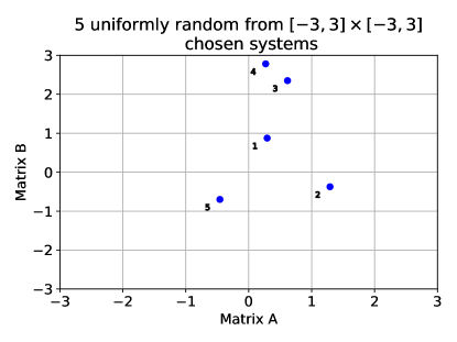
Refer to caption
Refer to caption
Refer to caption
Refer to caption
Refer to caption
Refer to caption
Figure 5: We sampled 5 systems and then computed the worse case performance on the systems within some radius around them. As we can see the robust controller can stabilize all systems within considerably larger radius around true system compared to CEC.

Appendix I Bounds discussion

We empirically observed that setting λ=2σw2Γ(n2+1)C2𝜆2superscriptsubscript𝜎𝑤2Γ𝑛21superscript𝐶2\lambda=\frac{2\sigma_{w}^{2}\Gamma(\frac{n}{2}+1)}{C^{2}} yields that credibility regions, with δ𝛿\delta probability of failure, contain systems with (A,B)FCsubscriptdelimited-∥∥subscript𝐴subscript𝐵𝐹𝐶\left\lVert(A_{*},B_{*})\right\rVert_{F}\leq C with empirical probability at least 1δ1𝛿1-\delta. Next we will motivate the decision behind such λ𝜆\lambda selection.

If the prior belief about the system is uniformly distributed over the set I={(A,B)|(AB)FC}𝐼conditional-set𝐴𝐵subscriptdelimited-∥∥𝐴𝐵𝐹𝐶I=\{(A,B)|\left\lVert(A~{}B)\right\rVert_{F}\leq C\}, then in order for prior Gaussian probability density function to be smaller or equal on I𝐼I than prior uniform probability density function we need to choose λ𝜆\lambda such that:

1(2π)n2(σw2λ)n2Γ(n2+1)πn2Cn,1superscript2𝜋𝑛2superscriptsuperscriptsubscript𝜎𝑤2𝜆𝑛2Γ𝑛21superscript𝜋𝑛2superscript𝐶𝑛\displaystyle\frac{1}{(2\pi)^{\frac{n}{2}}\left(\frac{\sigma_{w}^{2}}{\lambda}\right)^{\frac{n}{2}}}\leq\frac{\Gamma(\frac{n}{2}+1)}{\pi^{\frac{n}{2}}C^{n}},

which is satisfied if we select λ=2σw2Γ(n2+1)C2𝜆2superscriptsubscript𝜎𝑤2Γ𝑛21superscript𝐶2\lambda=\frac{2\sigma_{w}^{2}\Gamma(\frac{n}{2}+1)}{C^{2}}. As can be seen from Figure 6 this selection might not be the optimal one, however it seems that it at least captures the order of behavior λ1/C2𝜆1superscript𝐶2\lambda\approx 1/C^{2}.

The ultimate goal would be to obtain data dependent consistent (for regular systems) estimation error upper bounds in the frequentist setting. If we take as the estimators A^,B^^𝐴^𝐵\widehat{A},\widehat{B} the RLS with regularizing parameter λ𝜆\lambda one can show that:

((A^B^)(AB))superscript^𝐴^𝐵subscript𝐴subscript𝐵top\displaystyle\left((\widehat{A}~{}\widehat{B})-(A_{*}~{}B_{*})\right)^{\top} =(Vi+λI)1Siλ(Vi+λI)1(AB),absentsuperscriptsubscript𝑉𝑖𝜆𝐼1subscript𝑆𝑖𝜆superscriptsubscript𝑉𝑖𝜆𝐼1superscriptsubscript𝐴subscript𝐵top\displaystyle=\left(V_{i}+\lambda I\right)^{-1}S_{i}-\lambda\left(V_{i}+\lambda I\right)^{-1}(A_{*}~{}B_{*})^{\top},

where Vi=j=0i1zjzjsubscript𝑉𝑖superscriptsubscript𝑗0𝑖1subscript𝑧𝑗superscriptsubscript𝑧𝑗topV_{i}=\sum_{j=0}^{i-1}z_{j}z_{j}^{\top} and Si=j=0i1zjwj+1subscript𝑆𝑖superscriptsubscript𝑗0𝑖1subscript𝑧𝑗superscriptsubscript𝑤𝑗1topS_{i}=\sum_{j=0}^{i-1}z_{j}w_{j+1}^{\top}, with zj=(xjuj)subscript𝑧𝑗superscriptsuperscriptsubscript𝑥𝑗topsuperscriptsubscript𝑢𝑗toptopz_{j}=(x_{j}^{\top}u_{j}^{\top})^{\top}. Sarkar and Rakhlin (2019) showed that for regular systems (Vi+λI)1Siλ(Vi+λI)1(AB)2i0superscript𝑖subscriptdelimited-∥∥superscriptsubscript𝑉𝑖𝜆𝐼1subscript𝑆𝑖𝜆superscriptsubscript𝑉𝑖𝜆𝐼1superscriptsubscript𝐴subscript𝐵top20\left\lVert\left(V_{i}+\lambda I\right)^{-1}S_{i}-\lambda\left(V_{i}+\lambda I\right)^{-1}(A_{*}~{}B_{*})^{\top}\right\rVert_{2}\stackrel{{\scriptstyle i\to\infty}}{{\to}}0. However the term Sisubscript𝑆𝑖S_{i} is not observed. One could try and use the theory of Self-Normalizing Martingales and show that w.p. 1δ1𝛿1-\delta:

(Vi+λI)12Si228σw2log(det(Vi+λI)12det(λI)125dδ),subscriptsuperscriptdelimited-∥∥superscriptsubscript𝑉𝑖𝜆𝐼12subscript𝑆𝑖228superscriptsubscript𝜎𝑤2superscriptsubscript𝑉𝑖𝜆𝐼12superscript𝜆𝐼12superscript5𝑑𝛿\displaystyle\left\lVert(V_{i}+\lambda I)^{-\frac{1}{2}}S_{i}\right\rVert^{2}_{2}\leq 8\sigma_{w}^{2}\log\left(\frac{\det(V_{i}+\lambda I)^{\frac{1}{2}}}{\det(\lambda I)^{\frac{1}{2}}}\frac{5^{d}}{\delta}\right), (58)

however, since the norm of states xisubscript𝑥𝑖x_{i} can grow exponentially, one could show that the right hand side of Equation 58 can grow linearly and hence the upper bound on estimation error could be inconsistent. Sarkar and Rakhlin (2019) used the theory of Self-Normalizing Martingales to show that OLS is consistent, however instead of λI𝜆𝐼\lambda I in Equation 58 they inserted Vdnsubscript𝑉𝑑𝑛V_{dn} with VdnViprecedes-or-equalssubscript𝑉𝑑𝑛subscript𝑉𝑖V_{dn}\preceq V_{i}, however Vdnsubscript𝑉𝑑𝑛V_{dn} significantly depends on the system (A,B)𝐴𝐵(A,B) and is to the best of or knowledge not known how to obtain it in the data-dependent setting. How to get consistent data dependent upper bounds for the error term (Vi+λI)1Siλ(Vi+λI)1(AB)2subscriptdelimited-∥∥superscriptsubscript𝑉𝑖𝜆𝐼1subscript𝑆𝑖𝜆superscriptsubscript𝑉𝑖𝜆𝐼1superscriptsubscript𝐴subscript𝐵top2\left\lVert\left(V_{i}+\lambda I\right)^{-1}S_{i}-\lambda\left(V_{i}+\lambda I\right)^{-1}(A_{*}~{}B_{*})^{\top}\right\rVert_{2} is to the best of our knowledge also not known. However as we argued in Section 5, we observed empirically that with the right prior selection of λ𝜆\lambda, based on the knowledge of C𝐶C with (AB)FCsubscriptdelimited-∥∥subscript𝐴subscript𝐵𝐹𝐶\left\lVert(A_{*}~{}B_{*})\right\rVert_{F}\leq C, we can use Bayesian credibility regions ΘΘ\Theta.

{subfigure}

[dx=2,du=1formulae-sequencesubscript𝑑𝑥2subscript𝑑𝑢1d_{x}=2,d_{u}=1] Refer to caption {subfigure}[dx=du=2subscript𝑑𝑥subscript𝑑𝑢2d_{x}=d_{u}=2] Refer to caption {subfigure}[dx=du=3subscript𝑑𝑥subscript𝑑𝑢3d_{x}=d_{u}=3] Refer to caption

Figure 6: If we select λ𝜆\lambda as described above, it empirically turns out to be small enough, such that region ΘΘ\Theta contains A,Bsubscript𝐴subscript𝐵A_{*},B_{*}.

In the experiment presented in right most picture Figure 2 and Figure 6 we first selected different C𝐶C-s for which we computed the ”optimal” λ𝜆\lambda (λ𝜆\lambda presented on the figures as Empirical λ𝜆\lambda.) How we computed ”optimal” λ𝜆\lambda? Consider fixed C𝐶C and λ𝜆\lambda. We sampled 200200200 systems (AB)𝐴𝐵(A~{}B) uniformly at random from the set {(AB)|(AB)F=C}conditional-set𝐴𝐵subscriptdelimited-∥∥𝐴𝐵𝐹𝐶\{(A~{}B)|\left\lVert(A~{}B)\right\rVert_{F}=C\} and evolved each system for 10 steps. Then we computed the share of the steps when (AB)𝐴𝐵(A~{}B) were inside region ΘΘ\Theta. The ”optimal” λ𝜆\lambda is the largest λ𝜆\lambda where the share is larger than 1δ1𝛿1-\delta.