Sindy Löwe \Emailloewe.sindy@gmail.com
\addrUvA-Bosch Delta Lab, University of Amsterdam
and \NameDavid Madras \Emailmadras@cs.toronto.edu
\addrUniversity of Toronto, Vector Institute
and \NameRichard Zemel \Emailzemel@cs.toronto.edu
\addrUniversity of Toronto, Vector Institute
and \NameMax Welling \Emailwelling.max@gmail.com
\addrUvA-Bosch Delta Lab, University of Amsterdam
Amortized Causal Discovery:
Learning to Infer Causal Graphs from Time-Series Data
Abstract
On time-series data, most causal discovery methods fit a new model whenever they encounter samples from a new underlying causal graph. However, these samples often share relevant information which is lost when following this approach. Specifically, different samples may share the dynamics which describe the effects of their causal relations. We propose Amortized Causal Discovery, a novel framework that leverages such shared dynamics to learn to infer causal relations from time-series data. This enables us to train a single, amortized model that infers causal relations across samples with different underlying causal graphs, and thus leverages the shared dynamics information. We demonstrate experimentally that this approach, implemented as a variational model, leads to significant improvements in causal discovery performance, and show how it can be extended to perform well under added noise and hidden confounding.
keywords:
Causal Discovery, Granger Causality, Hidden Confounding, Noisy Observations, Amortization, Time-Series, Graph Neural Networks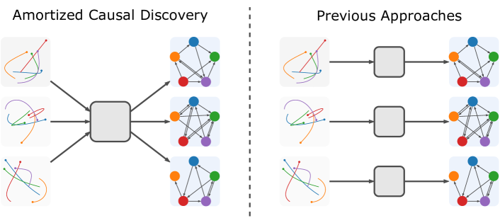
1 Introduction
Inferring causal relations in observational time-series is central to many fields of scientific inquiry (Spirtes et al., 2000; Berzuini et al., 2012). Suppose you want to analyze fMRI data, which measures the activity of different brain regions over time – how can you infer the (causal) influence of one brain region on another? This question is addressed by the field of causal discovery (Glymour et al., 2019). Methods within this field allow us to infer causal relations from observational data – when interventions (e.g. randomized trials) are infeasible, unethical or too expensive.
In time-series, the assumption that causes temporally precede their effects enables us to discover causal relations in observational data (Peters et al., 2017); with approaches relying on conditional independence tests (Entner and Hoyer, 2010), scoring functions (Chickering, 2002), or deep learning (Tank et al., 2018). All of these methods assume that samples share a single underlying causal graph and refit a new model whenever this assumption does not hold. However, samples with different underlying causal graphs may share relevant information, such as the dynamics describing the effects of causal relations. For instance, we may want to infer synaptic connections (i.e. causal relations) between neurons based on their spiking behavior, from a set of recordings of neuronal firing. Despite recording different populations of neurons with different wiring, the dynamics of how neurons connected by synapses influence one another may stay the same. This principle occurs in a number of areas: fMRI test subjects may have varying brain connectivity but the same underlying neurochemistry; social networks may have differing structure but comparable interpersonal relationships; different stocks may relate differently to one another but obey similar market forces. Despite a range of relevant applications, inferring causal relations across samples with different underlying causal graphs is as of yet largely unexplored.
In this paper, we propose a novel causal discovery framework for time-series that embraces this aspect: Amortized Causal Discovery (Fig. 1). In this framework, we learn to infer causal relations across samples with different underlying causal graphs but shared dynamics. We achieve this by separating the causal relation prediction from the modeling of their dynamics: an amortized encoder predicts the edges in the causal graph, and a decoder models the dynamics of the system under the predicted causal relations. This setup allows us to pool statistical strength across samples and to achieve significant improvements in performance with additional training data. It also allows us to infer causal relations in previously unseen samples without refitting our model. Additionally, we show that Amortized Causal Discovery can improve robustness under hidden confounding by modeling the unobserved variables with the amortized encoder. Our contributions are as follows:
-
•
We formalize Amortized Causal Discovery (ACD), a novel framework for causal discovery in time-series, in which we learn to infer causal relations from samples with different underlying causal graphs but shared dynamics (Eq. 2).
-
•
We propose a variational model for ACD, applicable to multi-variate, non-linear data.
-
•
We present experiments demonstrating the effectiveness of this model on a range of causal discovery datasets, in the fully observed setting, with added noise, and under hidden confounding.
2 Background: Granger Causality
Granger causality (Granger, 1969) is one of the most commonly used approaches to infer causal relations from observational time-series data. Its central assumption is that causes precede their effects: if the prediction of the future of time-series can be improved by knowing past elements of time-series , then “Granger causes” . Originally, Granger causality was defined for linear relations; we follow the more recent definition of Tank et al. (2018) for non-linear Granger causality:
Definition 2.1.
Non-Linear Granger Causality: Given stationary time-series across time-steps and a non-linear autoregressive function , such that
| (1) |
where denotes the present and past of series and represents independent noise.
In this setup, time-series Granger causes , if depends on , i.e. if
.
Granger causal relations are equivalent to causal relations in the underlying directed acyclic graph (DAG) if all relevant variables are observed and no instantaneous111connections between two variables at the same time step connections exist (Peters et al., 2013, 2017, Theorem 10.1).
Many methods for Granger causal discovery, including vector autoregressive (Hyvärinen et al., 2010) and more recent deep learning-based approaches (Tank et al., 2018; Khanna and Tan, 2019; Wu et al., 2020), can be encapsulated by a particular framework:
- 1.
-
2.
Fit to by minimizing some loss : .
-
3.
Apply some fixed function (e.g. thresholding) to the learned parameters to produce the Granger causal graph estimate for : . For instance, Tank et al. (2018) infer the Granger causal relations through examination of the weights : if all outgoing weights between time-series and are zero, then does not Granger-cause .
The shortcoming of this approach is that, when we have samples with different underlying causal graphs, the parameters must be optimized separately for each of them. As a result, methods within this framework cannot take advantage of the information that might be shared between samples. This motivates us to question: can we amortize this process?
3 Amortized Causal Discovery
We propose Amortized Causal Discovery (ACD), a framework in which we learn to infer causal relations across samples with different underlying causal graphs but shared dynamics. To illustrate, we return to the example from Section 1: suppose you want to infer synaptic connections (i.e. causal relations) between neurons based on their spiking behavior. You are given a set of recordings (i.e. samples), each containing time-series representing the firing of individual neurons. Even though you might record across different populations of neurons with different wiring, the dynamics of how neurons connected by synapses influence one another stays the same. ACD takes advantage of such shared dynamics to improve the prediction of causal relations. Given a training set and test sequence , it can be summarized as follows:
-
1.
Define an encoding function which learns to infer Granger causal relations of any sample in . Define a decoding function which learns to predict the next time-step of the samples under the inferred causal relations.
-
2.
Fit and to by minimizing some loss : .
-
3.
For a test sequence , simply output the Granger causal graph estimate :
.
By dividing the model into two parts, an encoder and a decoder, ACD can use the activations of to infer causal structure. This increases the flexibility of our approach greatly compared to methods that use the learned weights such as the prior Granger causal discovery methods described in Section 2. In this section, we describe our framework in more detail, and provide a probabilistic implementation thereof. We also extend our approach to model hidden confounders.
Preliminaries
We begin with a dataset of samples, where each sample consists of stationary time-series across time-steps . We denote the -th time-step of the -th time-series of as (sometimes omitting for brevity). We assume there is an associated directed acyclic graph underlying the generative process of each sample. This is a structural causal model (SCM) (Pearl, 2009). Its endogenous (observed) variables are vertices for each time-series and each time-step . Every set of incoming edges to an endogenous variable defines inputs to a deterministic function which determines that variable’s value222The SCM also includes an exogenous (unobserved), independently-sampled error variable as a parent of each vertex , which we do not model and thus leave out for brevity.. The edges are defined by ordered pairs of vertices , which we make two assumptions about:
-
1.
No edges are instantaneous () or go back in time. Thus, for all edges.
-
2.
Edges are invariant to time. Thus, if , then . The associated structural equations are invariant to time as well, i.e. .
The first assumption states that causes temporally precede their effects and makes causal relations identifiable from observational data, when no hidden confounders are present (Peters et al., 2013, 2017, Theorem 10.1). The second simplifies modeling: it is a fairly general assumption that allows us to define dynamics that govern all time-steps (Eq. 2).
Throughout this paper, we are interested in discovering the summary graph (Peters et al., 2017). It consists of vertices for each time-series in sample , and has directed edges whenever they exist in at any time-step, i.e. . Note that while is acyclic (due to the first assumption above), the summary graph may contain (self-)cycles.
Amortized Causal Discovery
The key assumption for Amortized Causal Discovery is that there exists some fixed function that describes the dynamics of all samples given their past observations and their underlying causal graph :
| (2) |
There are two variables in this data-generating process that we would like to model: the causal graph that is specific to sample , and the dynamics that are shared across all samples. This separation between the causal graph and the dynamics allows us to divide our model accordingly: we introduce an amortized causal discovery encoder which learns to infer a causal graph given the sample , and a dynamics decoder that learns to approximate :
| (3) |
We formalize Amortized Causal Discovery (ACD) as follows. Let be the domain of all possible summary graphs on : . Let be the domain of any single step, partial or full, observed sequence: . The model consists of two components: a causal discovery encoder which infers a causal graph for each input sample, and a decoder which models the dynamics. This model is optimized with a sample-wise loss which scores how well the decoder models the true dynamics of , and a regularization term on the inferred graphs. For example, this function may enforce sparsity by penalizing graphs with more edges. Note, that our formulation of the graph prediction problem is unsupervised: we do not have access to the true underlying graph . Then, given some dataset with samples, we optimize:
| (4) | ||||
| (5) |
Once we have completed optimization, we can perform causal graph prediction on any new input test sample in two ways – we can feed into the amortized encoder and take its output as the predicted edges (Eq. 6); or we can instantiate our estimate which will be our edge predictions, and find the edges which best explain the observed sequence by minimizing the (learned) decoding loss with respect to , which we term Test-Time Adaptation (TTA) (Eq. 7):
| (6) | ||||
| (7) |
By separating the prediction of causal relations from the modeling of their dynamics, ACD yields a number of benefits. ACD can learn to infer causal relations across samples with different underlying causal graphs, and it can infer causal relations in previously unseen test samples without refitting (Eq. 6). By generalizing across samples, it can improve causal discovery performance with increasing training data size. We can replace either or with ground truth annotations, or simulate the outcome of counterfactual causal relations. Additionally, ACD can be applied in the standard causal discovery setting, where only a single causal graph underlies all samples, by replacing the amortized encoder with an estimated graph (or distribution over ) in Eq. 4.
3.1 A Probabilistic Implementation of ACD

We take a probabilistic approach to ACD and model the functions and using variational inference (Fig. 2). We amortize the encoder with an encoding function , which outputs a distribution over representing the predicted edges in the causal graph; and we learn a decoder which probabilistically models the dynamics of the time-series under the predicted causal relations. We choose a negative log-likelihood for the decoder loss and a KL-Divergence to a prior distribution over for the regularizer . As a result, our loss function is a variational lower bound:
| (8) |
Encoder
The encoder applies a graph neural network (Scarselli et al., 2008; Li et al., 2016; Gilmer et al., 2017; Kipf and Welling, 2017) to the input, which propagates information across a fully connected graph . This graph includes vertices for each time-series , and each pair of vertices is connected by an edge.
| (9) | ||||
| (10) | ||||
| To enable us to backpropagate through the samples of the discrete distribution , during training, we relax it by adding Gumbel distributed noise (Maddison et al., 2017; Jang et al., 2017): | ||||
| (11) | ||||
The output of the encoder represents the predicted edges in the causal graph . We consider the possibility that there are different edge-types expressing causal relationships; for instance, inhibitory or excitatory synaptic connections. Then, more specifically, expresses that there is a directed edge of type from time-series to , where .
Decoder
The decoder models the dynamics of the time-series under the predicted causal relations. It uses both the predicted causal relations and the feature vectors of the time-series at the current time-step , as its input. First, it propagates information along the predicted edges by applying a neural network , using the zero function for :
| (12) |
Then, the decoder accumulates the incoming messages to each node and applies a neural network to predict the change between the current and the next time-step:
| (13) | ||||
| (14) |
In other words, the decoder predicts , which is added to the current value of the time-series to yield the prediction for the next time-step . Note that this approach assumes the existence of self-edges: that is, the value of always affects the value of .
Prediction of Causal Relations
In order to align our model with the philosophy of Granger Causality, we include a “no edge”-type edge function: If the encoder predicts the “no edge”-type edge by setting , the decoder uses the zero function and no information is propagated from time-series to (Eq. 12). Due to this, time-series will Granger cause the decoder-predicted time-series only when the edge is predicted to exist (see Appendix A). Hence, by the same logic that justifies prior Granger causal work (Section 2), we expect the predicted edges to correspond to Granger causal relations. Finally, since we assume no hidden confounders and no instantaneous edges, these Granger causal relations will correspond to relations in the underlying SCM (Peters et al., 2017, Theorem 10.3).
3.2 Hidden Confounding
Hidden confounders are a critical problem in the time-series context: when they exist, Granger causality is not guaranteed to correspond to the true causal graph anymore (Peters et al., 2017, Theorem 10.3)333For instance, if an unobserved time-series causes both time-series and , then the past of can help predict the future of , even though there is no causal link between them.. Inspired by proxy-based methods from causal inference (e.g. Louizos et al. (2017), see Section 4), we present a method for applying ACD to the hidden confounding setting. First, we extend the amortized encoder to predict an additional variable. Then, we encourage this variable to model the hidden confounder by applying a structural bias – depending on the type of unobserved variable that we want to model, its predicted value is utilized differently by the remaining model. The decoder remains responsible for modeling the dynamics, and now also processes the predictions for the unobserved variable. While this setup might not allow us to identify the hidden confounders, and it is still true that the predicted Granger causal relations may not correspond to the underlying SCM, the data-driven approach underlying ACD can benefit our model: by training across samples with different underlying causal graphs, our model has access to substantially more information about the causal dynamics at hand and we show empirically that it can learn to mitigate the effects of the hidden confounders.
We consider two types of hidden confounders which were chosen to cover a wide range of potential confounders as one might encounter in practice. First, we introduce a temperature variable that confounds all observed variables by influencing the strength of their causal relations. This temperature is sampled separately for each sample, and remains constant throughout each sample. This is a realistic example of a global variable that may influence physical dynamics. Second, we introduce a hidden variable that behaves just like the observed variables, i.e. it may affect or be affected by the observed variables through the same causal relations, and its value changes across time. This confounder is inspired by the introductory example where one wants to infer the causal relations between neurons based on their spiking pattern. In this scenario, it is virtually impossible to record all relevant neurons. The resulting unobserved neurons behave and influence the observed neurons in a similar fashion as the unobserved time-series confounder introduced here. In both scenarios, we extend the encoder to predict this hidden variable, and feed that prediction into the decoder. We provide more details in Section 5.2.
4 Related Work
A range of approaches to causal discovery in both temporal and non-temporal data exist (Heinze-Deml et al., 2018; Spirtes et al., 2000; Peters et al., 2017). One common class is constraint-based, relying on conditional independence testing to uncover an underlying DAG structure or equivalence class (Spirtes et al., 2000). These methods predict a single graph (or equivalence class) for all samples. There is no notion of fitting a dynamics model for time-series methods in this class (Entner and Hoyer, 2010). Another common class of methods for causal discovery is score-based (Chickering, 2002; Bengio et al., 2019). Here, a score function is chosen, and the methods perform a search through graph space to optimize this score, i.e. . Our proposed decoder-based inference (Eq. 7) can be seen as score-based causal discovery with a learned score function . A third class of methods fits a (possibly regularized) dynamics model and then analyzes its form to produce a causal graph estimate, by using linear dynamics (Hyvärinen et al., 2010), recurrent models (Tank et al., 2018; Khanna and Tan, 2019; Nauta et al., 2019), or other deep-learning based approaches (Wu et al., 2020; Lachapelle et al., 2019; Zheng et al., 2020). See Section 2 for discussion.
The range of approaches to causal discovery relevant to ours include Li et al. (2018), who propose to learn a linear mixed effects model across samples; concurrent work explores amortized deep learning of differing types of causal structure (Li et al., 2020; Ke et al., 2020) and the relationship between GNNs and causal effect inference (Zečević et al., 2021). Additionally relevant are other approaches for temporal data: works such as Peters et al. (2013) or Eichler (2012) use independence or additivity assumptions. Another adjacent category of causal discovery work explores the idea of jointly learned causal structure across examples, including in the setting where a number of related datasets are collected (Dhir and Lee, 2020; Huang et al., 2019, 2020b; Shimizu, 2012; Tillman and Eberhardt, 2014; Huang et al., 2020a).
There is little systematic study of hidden confounding in the time-series setting. Some empirical work in the non-temporal domain shows that encoder-based models with enough proxies (variables caused by hidden confounders) can improve causal inference under hidden confounding (Louizos et al., 2017; Parbhoo et al., 2020), and theoretical work proves the identifiability of latent variables from proxies under some assumptions (Kruskal, 1977; Allman et al., 2009).
Several works have used graph neural networks (Battaglia et al., 2016; Santoro et al., 2017; Kipf et al., 2018) or attention mechanisms (Vaswani et al., 2017; Fuchs et al., 2019; Goyal et al., 2019; Van Steenkiste et al., 2018) to infer relations between time-series. Alet et al. (2019) propose a meta-learning algorithm to additionally model unobserved variables. While these approaches model object relations in a number of ways, they are not explicitly designed to infer causal graphical structure.
The probabilistic implementation of ACD is based on the Neural Relational Inference (NRI) model (Kipf et al., 2018). We extend this work by new inference methods using test-time adaptation and new algorithms to handle hidden confounders. Moreover, we provide a proof that relates the zero-edge function to Granger causality, which allows for a causal interpretation of the inferred edges. Subsequently, we apply our model to a different problem than NRI, namely (Granger) causal discovery, and show that it outperforms the current state of the art for this type of problem. Last but not least, we show that our model achieves strong causal discovery performance even under noise and hidden confounding, an accomplishment that is – to the best of our knowledge – new in this field.
5 Experiments
Implementation
We measure causal discovery performance by the area under the receiver operator curve (AUROC) of predicted edge probabilities over test samples. We compare to recurrent models (Tank et al. (2018); Khanna and Tan (2019)), a mutual-information (MI) based model by Wu et al. (2020) and several baselines implemented by those authors, including MI (unmodified), transfer entropy (Schreiber, 2000), and linear Granger causality. More details in Appendix B, our code is available at github.com/loeweX/AmortizedCausalDiscovery.
5.1 Fully Observed Amortized Causal Discovery
We test ACD on three datasets: two fully-observed physics simulations (Kuramoto and Particles) and the Netsim dataset of simulated fMRI data (Smith et al., 2011). Note, in contrast to the physics simulations used in Kipf et al. (2018), we generate data with asymmetric connectivity matrices to represent causal relations.
First, we test our method on the Kuramoto dataset, which contains five 1-D time-series of phase-coupled oscillators (Kuramoto, 1975). We find that ACD greatly outperforms all approaches for Granger causal discovery that we compare against (Table 1). In contrast to these approaches, ACD achieves this result without fitting to the test samples.
| Method | AUROC |
| MPIR (Wu et al., 2020) | 0.502 0.006 |
| Transfer Entropy (Schreiber, 2000) | 0.560 0.005 |
| NGC (Tank et al., 2018) | 0.574 0.018 |
| eSRU (Khanna and Tan, 2019) | 0.607 0.001 |
| Mutual Information | 0.616 0.000 |
| Linear Granger Causality | 0.647 0.003 |
| Amortized Causal Discovery | 0.952 0.003 |
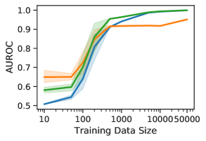
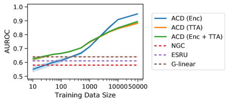
Additionally, we find that ACD can indeed utilize samples with different underlying causal graphs – its performance improves steadily with increasing training data size (Fig. 3). Nonetheless, it is also applicable to the low-data regime: when applying ACD with test-time adaptation (TTA), it requires less than training samples to outperform all previous approaches. We note that the baseline performance here is worse than presented elsewhere in the literature – this is because we do not evaluate the prediction of self-connectivity, which is the easiest connectivity to predict.
In our second experiment, we apply ACD to the particles dataset. This dataset models five particles that move around a two-dimensional space, with some particles influencing others uni-directionally by pulling them with a spring. Since all previous methods were intended for one-dimensional time-series, we were unable to evaluate them in this domain. ACD, on the other hand, is readily applicable to higher-dimensional data, and performs almost perfectly on this dataset with 0.999 AUROC.
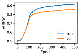
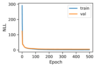
In both experiments, causal relation prediction with the learned encoder (Enc - Eq. 6) performs best in the high-data regime, while test-time adaptation (TTA - Eq. 7) improves the performance in low-data settings (Fig. 3). This benefit of TTA can be largely attributed to two effects. First, TTA closes the amortization gap of the encoder (Cremer et al., 2018). Second, TTA overcomes the encoder’s overfitting on the training data (as seen in the training curves in Section B.2) by adapting to the individual test samples. On the particles dataset, initializing TTA with the encoder’s prediction (Enc+TTA) improves over a random initialization (TTA) as the encoder improves; but we do not observe this effect on the Kuramoto dataset.
| Method | AUROC |
| MPIR (Wu et al., 2020) | 0.484 0.017 |
| Transfer Entropy (Schreiber, 2000) | 0.543 0.003 |
| NGC (Tank et al., 2018) | 0.624 0.020 |
| eSRU (Khanna and Tan, 2019) | 0.670 0.015 |
| Mutual Information | 0.728 0.002 |
| Linear Granger Causality | 0.503 0.004 |
| Amortized Causal Discovery | 0.688 0.051 |
Finally, we apply ACD to the Netsim dataset (Smith et al., 2011) of simulated fMRI data. Here, the task is to infer the underlying connectivity between 15 brain regions across 50 samples. A single graph underlies all samples, allowing us to demonstrate ACD’s applicability to the classical setting. We replace the amortized encoder with a global latent distribution , optimize it through the decoder, and then use test-time adaptation (TTA). Even though our model cannot benefit from its data-driven design here, it performs comparably to methods that are intended for use in the single-graph setting (Table 2).
5.1.1 Noisy Data
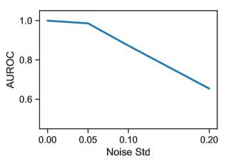
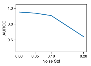
Handling noisy data is a key challenge in causal discovery. Here, we show that ACD is robust to a certain amount of observational noise in both the Particles and Kuramoto tasks.
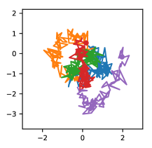
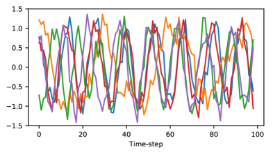
We test ACD’s performance for different levels of observation noise added to the Particles and Kuramoto datasets (see Fig. 8 in the Appendix for visual examples). We sample this additive noise from a zero-mean normal distribution with standard deviations varying between 0.0 and 0.2. For comparison, the input samples in both the Particles and Kuramoto datasets have a standard deviation of 0.6. For each dataset and each standard deviation, we train across five random seeds. In Fig. 4, we show the average AUROC on a test set with the same noise scheme applied. ACD’s performance degrades gracefully when stronger observation noise is added. In the highest noise scenario, when the noise is sampled from a normal distribution with a standard deviation of 0.2, the performance of ACD matches the performance of the baselines from Table 1 on noiseless data.
[0.48]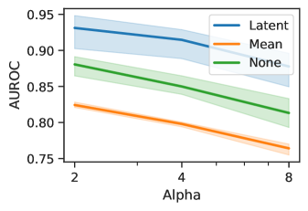 \ffigbox[0.48]
5.2 Amortized Causal Discovery under Hidden Confounding
5.2.1 Latent Temperature
In this experiment, we use the particles dataset and vary an unobserved temperature variable, which modulates how strongly the particles exert force on each other – higher temperatures result in stronger forces and a more chaotic system. For each , we sample an independent temperature from a categorical distribution with and equal probabilities. We predict this unobserved temperature by extending the amortized encoder with an additional latent variable, which models a uniform distribution. Then, we add a KL-Divergence between this posterior and a uniform prior on the interval to our variational loss. To allow for learning in this setting, we introduce an inductive bias: we use a decoder which matches the true dynamics given the predicted temperature and causal relations. See Section C.1 for more details and additional results.
Results
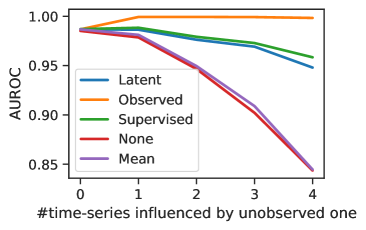
Fig. 6 shows the causal discovery results across different values of . ACD enhanced with an additional latent variable (Latent) outperforms both tested baselines across all temperatures: Mean, which uses the same ground-truth decoder as Latent and fixes the decoder temperature to be the mean of the categorical distribution, and None, which does not model explicitly and trains an MLP decoder. Additionally, this method achieves high predictive performance on the unobserved temperature variable: for = 2, temperature prediction obtains 0.888 , 0.966 AUROC and 0.644 accuracy. These results indicate that we can model an unobserved temperature variable, and thus improve robustness under hidden confounding.
5.2.2 Unobserved Time-Series

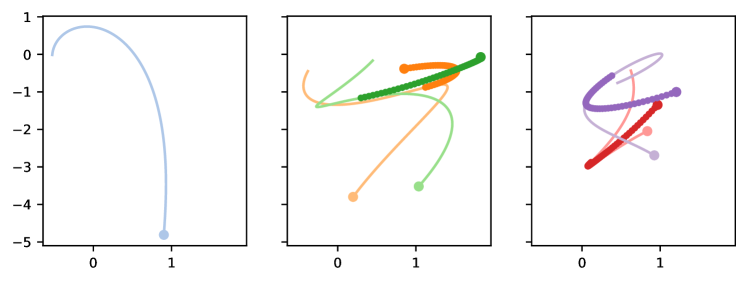
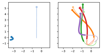
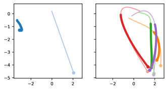
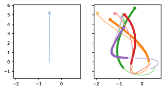
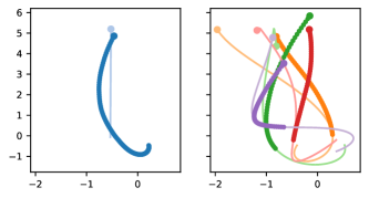
Here, we treat one of the original time-series in the particles dataset as unobserved. It exhibits the same dynamics as the observed time-series, evolving and causally influencing others the same way as before. This challenging setting has received little attention in the literature; Alet et al. (2019) tackled it with mixed success. We model the unobserved time-series by extending the amortized encoder with an additional latent variable and applying a suitable structural bias: the latent prediction for time-steps is treated in the same way as the observed time-series . Its entire trajectory is used by the encoder to predict causal relations, and its value at the current time-step is fed into the decoder. See Section C.2 for more details and additional results.
Results
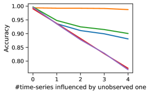
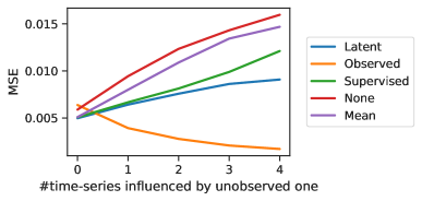
Fig. 6 shows how the causal discovery AUROC depends on the number of observed time-series directly influenced by the unobserved one. When this number is zero, all tested approaches perform the same. With growing numbers of influenced time-series, the baselines that either ignore the missing time-series (None) or impute its value with the average of the observed time-series over time (Mean) deteriorate strongly. In contrast, the proposed ACD with a Latent variable stays closer to the performance of the fully Observed baseline. As shown in Fig. 7, it also improves the future trajectory prediction of the observed time-series. A Supervised baseline, that uses the (usually unavailable) ground-truth trajectories to optimize the prediction of the unobserved time-series, improves only slightly over our approach. These results indicate that ACD can use latent variables to improve robustness to unobserved time-series.
6 Conclusion
We introduce ACD, a framework for causal discovery in time-series data which can leverage the information that is shared across samples. We provide a probabilistic implementation of this framework, and demonstrate significant performance gains over the existing literature when predicting causal relations, both in the fully observed setting and with noise and hidden confounding.
Despite this improvement in performance over previous work, several limitations remain. Our assumptions from Sec. 3 regarding shared dynamics and edges in the graph, are not verifiable in practice; however, this is standard in causal inference, which frequently relies on untestable assumptions such as ignorability or consistency.
We conducted all our experiments on simulated data; as a result, they are not particularly realistic: real-world data is more complex and potentially misspecified. This limitation is in line with the data used in related works (e.g. Khanna and Tan (2019)), and it remains an exciting direction for future work to improve modeling and experimentation in more realistic settings.
Finally, our contribution is primarily empirical: we propose and attack a novel version of the causal discovery problem – where samples have different underlying causal graphs but shared dynamics – and demonstrate that ACD outperforms prior methods by a large margin in this setting. It remains an important future direction of inquiry to understand the conditions under which ACD, as well as other Granger causal discovery approaches that inspired ACD (e.g. Tank et al. (2018); Khanna and Tan (2019)), can be guaranteed to identify the correct causal structures. \acksThanks to Thomas Kipf for helpful discussions and to Sara Magliacane, Marco Federici, Gabriele Bani, Joop Pascha, Patrick Forre, Pascal Esser, Maja Rudolph, Elliot Creager, Taylor Killian, and Renjie Liao for their feedback on the manuscript. David Madras was supported by an NSERC Alexander Graham Bell Canada Graduate Scholarship-Doctoral (CGS-D). Resources used in preparing this research were provided, in part, by the Province of Ontario, the Government of Canada through CIFAR, and companies sponsoring the Vector Institute (www.vectorinstitute.ai/#partners).
References
- Alet et al. (2019) Ferran Alet, Erica Weng, Tomás Lozano-Pérez, and Leslie Pack Kaelbling. Neural relational inference with fast modular meta-learning. In Advances in Neural Information Processing Systems, pages 11804–11815, 2019.
- Allman et al. (2009) Elizabeth S Allman, Catherine Matias, John A Rhodes, et al. Identifiability of parameters in latent structure models with many observed variables. The Annals of Statistics, 37(6A):3099–3132, 2009.
- Battaglia et al. (2016) Peter Battaglia, Razvan Pascanu, Matthew Lai, Danilo Jimenez Rezende, et al. Interaction networks for learning about objects, relations and physics. In Advances in Neural Information Processing Systems, pages 4502–4510, 2016.
- Bengio et al. (2019) Yoshua Bengio, Tristan Deleu, Nasim Rahaman, Nan Rosemary Ke, Sebastien Lachapelle, Olexa Bilaniuk, Anirudh Goyal, and Christopher Pal. A meta-transfer objective for learning to disentangle causal mechanisms. In International Conference on Learning Representations, 2019.
- Berzuini et al. (2012) Carlo Berzuini, Philip Dawid, and Luisa Bernardinell. Causality: Statistical perspectives and applications. John Wiley & Sons, 2012.
- Chickering (2002) David Maxwell Chickering. Optimal structure identification with greedy search. Journal of Machine Learning Research, 3(Nov):507–554, 2002.
- Cremer et al. (2018) Chris Cremer, Xuechen Li, and David Duvenaud. Inference suboptimality in variational autoencoders. In International Conference on Machine Learning, pages 1078–1086, 2018.
- Dhir and Lee (2020) Anish Dhir and Ciarán M Lee. Integrating overlapping datasets using bivariate causal discovery. In AAAI, pages 3781–3790, 2020.
- Eichler (2012) Michael Eichler. Causal inference in time series analysis. Wiley Online Library, 2012.
- Entner and Hoyer (2010) Doris Entner and Patrik O Hoyer. On causal discovery from time series data using FCI. Probabilistic Graphical Models, pages 121–128, 2010.
- Fuchs et al. (2019) Fabian B Fuchs, Adam R Kosiorek, Li Sun, Oiwi Parker Jones, and Ingmar Posner. End-to-end recurrent multi-object tracking and trajectory prediction with relational reasoning. arXiv preprint arXiv:1907.12887, 2019.
- Gilmer et al. (2017) Justin Gilmer, Samuel S Schoenholz, Patrick F Riley, Oriol Vinyals, and George E Dahl. Neural message passing for quantum chemistry. In International Conference on Machine Learning, pages 1263–1272, 2017.
- Glymour et al. (2019) Clark Glymour, Kun Zhang, and Peter Spirtes. Review of causal discovery methods based on graphical models. Frontiers in Genetics, 10, 2019.
- Goyal et al. (2019) Anirudh Goyal, Alex Lamb, Jordan Hoffmann, Shagun Sodhani, Sergey Levine, Yoshua Bengio, and Bernhard Schölkopf. Recurrent independent mechanisms. arXiv preprint arXiv:1909.10893, 2019.
- Granger (1969) Clive WJ Granger. Investigating causal relations by econometric models and cross-spectral methods. Econometrica: Journal of the Econometric Society, pages 424–438, 1969.
- Heinze-Deml et al. (2018) Christina Heinze-Deml, Marloes H Maathuis, and Nicolai Meinshausen. Causal structure learning. Annual Review of Statistics and Its Application, 5:371–391, 2018.
- Hochreiter and Schmidhuber (1997) Sepp Hochreiter and Jürgen Schmidhuber. Long short-term memory. Neural Computation, 9(8):1735–1780, 1997.
- Huang et al. (2019) Biwei Huang, Kun Zhang, Pengtao Xie, Mingming Gong, Eric P Xing, and Clark Glymour. Specific and shared causal relation modeling and mechanism-based clustering. In Advances in Neural Information Processing Systems, pages 13510–13521, 2019.
- Huang et al. (2020a) Biwei Huang, Kun Zhang, Mingming Gong, and Clark Glymour. Causal discovery from multiple data sets with non-identical variable sets. In AAAI, pages 10153–10161, 2020a.
- Huang et al. (2020b) Biwei Huang, Kun Zhang, Jiji Zhang, Joseph D Ramsey, Ruben Sanchez-Romero, Clark Glymour, and Bernhard Schölkopf. Causal discovery from heterogeneous/nonstationary data. J. Mach. Learn. Res., 21(89):1–53, 2020b.
- Hyvärinen et al. (2010) Aapo Hyvärinen, Kun Zhang, Shohei Shimizu, and Patrik O. Hoyer. Estimation of a structural vector autoregression model using non-gaussianity. Journal of Machine Learning Research, 11(56):1709–1731, 2010.
- Jang et al. (2017) Eric Jang, Shixiang Gu, and Ben Poole. Categorical reparametrization with gumble-softmax. In International Conference on Learning Representations, 2017.
- Ke et al. (2020) Nan Rosemary Ke, Jane Wang, Jovana Mitrovic, Martin Szummer, Danilo J Rezende, et al. Amortized learning of neural causal representations. arXiv preprint arXiv:2008.09301, 2020.
- Khanna and Tan (2019) Saurabh Khanna and Vincent YF Tan. Economy statistical recurrent units for inferring nonlinear granger causality. International Conference on Learning Representations, 2019.
- Kingma and Ba (2015) Diederik P Kingma and Jimmy Ba. Adam: A method for stochastic optimization. In International Conference on Learning Representations, 2015.
- Kipf and Welling (2017) Thomas Kipf and Max Welling. Semi-supervised classification with graph convolutional networks. In International Conference on Learning Representations, 2017.
- Kipf et al. (2018) Thomas Kipf, Ethan Fetaya, Kuan-Chieh Wang, Max Welling, and Richard Zemel. Neural relational inference for interacting systems. In International Conference on Machine Learning, pages 2688–2697, 2018.
- Kruskal (1977) Joseph B Kruskal. Three-way arrays: rank and uniqueness of trilinear decompositions, with application to arithmetic complexity and statistics. Linear Algebra and its Applications, 18(2):95–138, 1977.
- Kuramoto (1975) Yoshiki Kuramoto. Self-entrainment of a population of coupled non-linear oscillators. In International Symposium on Mathematical Problems in Theoretical Physics, pages 420–422. Springer, 1975.
- Lachapelle et al. (2019) Sébastien Lachapelle, Philippe Brouillard, Tristan Deleu, and Simon Lacoste-Julien. Gradient-based neural dag learning. In International Conference on Learning Representations, 2019.
- Li et al. (2018) Xiang Li, Shanghong Xie, Peter McColgan, Sarah J Tabrizi, Rachael I Scahill, Donglin Zeng, and Yuanjia Wang. Learning subject-specific directed acyclic graphs with mixed effects structural equation models from observational data. Frontiers in genetics, 9:430, 2018.
- Li et al. (2016) Yujia Li, Daniel Tarlow, Marc Brockschmidt, and Richard Zemel. Gated graph sequence neural networks. In International Conference on Learning Representations, 2016.
- Li et al. (2020) Yunzhu Li, Antonio Torralba, Animashree Anandkumar, Dieter Fox, and Animesh Garg. Causal discovery in physical systems from videos. arXiv preprint arXiv:2007.00631, 2020.
- Lin et al. (2017) Zhouhan Lin, Minwei Feng, Cicero Nogueira dos Santos, Mo Yu, Bing Xiang, Bowen Zhou, and Yoshua Bengio. A structured self-attentive sentence embedding. In International Conference on Learning Representations, 2017.
- Louizos et al. (2017) Christos Louizos, Uri Shalit, Joris M Mooij, David Sontag, Richard Zemel, and Max Welling. Causal effect inference with deep latent-variable models. In Advances in Neural Information Processing Systems, pages 6446–6456, 2017.
- Maddison et al. (2017) Chris J Maddison, Andriy Mnih, and Yee Whye Teh. The concrete distribution: A continuous relaxation of discrete random variables. In International Conference on Learning Representations, 2017.
- Nauta et al. (2019) Meike Nauta, Doina Bucur, and Christin Seifert. Causal discovery with attention-based convolutional neural networks. Machine Learning and Knowledge Extraction, 1(1):312–340, 2019.
- Parbhoo et al. (2020) Sonali Parbhoo, Mario Wieser, Aleksander Wieczorek, and Volker Roth. Information bottleneck for estimating treatment effects with systematically missing covariates. Entropy, 22(4):389, 2020.
- Paszke et al. (2019) Adam Paszke, Sam Gross, Francisco Massa, Adam Lerer, James Bradbury, Gregory Chanan, Trevor Killeen, Zeming Lin, Natalia Gimelshein, Luca Antiga, et al. PyTorch: An imperative style, high-performance deep learning library. In Advances in Neural Information Processing Systems, pages 8024–8035, 2019.
- Pearl (2009) Judea Pearl. Causality. Cambridge University Press, 2009.
- Peters et al. (2013) Jonas Peters, Dominik Janzing, and Bernhard Schölkopf. Causal inference on time series using restricted structural equation models. In Advances in Neural Information Processing Systems, pages 154–162, 2013.
- Peters et al. (2017) Jonas Peters, Dominik Janzing, and Bernhard Schölkopf. Elements of causal inference: foundations and learning algorithms. MIT Press, 2017.
- Santoro et al. (2017) Adam Santoro, David Raposo, David G Barrett, Mateusz Malinowski, Razvan Pascanu, Peter Battaglia, and Timothy Lillicrap. A simple neural network module for relational reasoning. In Advances in Neural Information Processing Systems, pages 4967–4976, 2017.
- Scarselli et al. (2008) Franco Scarselli, Marco Gori, Ah Chung Tsoi, Markus Hagenbuchner, and Gabriele Monfardini. The graph neural network model. IEEE Transactions on Neural Networks, 20(1):61–80, 2008.
- Schreiber (2000) Thomas Schreiber. Measuring information transfer. Physical Review Letters, 85(2):461, 2000.
- Shimizu (2012) Shohei Shimizu. Joint estimation of linear non-gaussian acyclic models. Neurocomputing, 81:104–107, 2012.
- Smith et al. (2011) Stephen M Smith, Karla L Miller, Gholamreza Salimi-Khorshidi, Matthew Webster, Christian F Beckmann, Thomas E Nichols, Joseph D Ramsey, and Mark W Woolrich. Network modelling methods for fMRI. Neuroimage, 54(2):875–891, 2011.
- Spirtes et al. (2000) Peter Spirtes, Clark N Glymour, Richard Scheines, and David Heckerman. Causation, prediction, and search. MIT Press, 2000.
- Tank et al. (2018) Alex Tank, Ian Covert, Nicholas Foti, Ali Shojaie, and Emily Fox. Neural granger causality for nonlinear time series. arXiv preprint arXiv:1802.05842, 2018.
- Tillman and Eberhardt (2014) Robert E Tillman and Frederick Eberhardt. Learning causal structure from multiple datasets with similar variable sets. Behaviormetrika, 41(1):41–64, 2014.
- Van Steenkiste et al. (2018) Sjoerd Van Steenkiste, Michael Chang, Klaus Greff, and Jürgen Schmidhuber. Relational neural expectation maximization: Unsupervised discovery of objects and their interactions. In International Conference on Learning Representations, 2018.
- Vaswani et al. (2017) Ashish Vaswani, Noam Shazeer, Niki Parmar, Jakob Uszkoreit, Llion Jones, Aidan N Gomez, Łukasz Kaiser, and Illia Polosukhin. Attention is all you need. In Advances in Neural Information Processing Systems, pages 5998–6008, 2017.
- Wu et al. (2020) Tailin Wu, Thomas Breuel, Michael Skuhersky, and Jan Kautz. Discovering nonlinear relations with minimum predictive information regularization. arXiv preprint arXiv:2001.01885, 2020.
- Zečević et al. (2021) Matej Zečević, Devendra Singh Dhami, Petar Veličković, and Kristian Kersting. Relating graph neural networks to structural causal models. arXiv preprint arXiv:2109.04173, 2021.
- Zheng et al. (2020) Xun Zheng, Chen Dan, Bryon Aragam, Pradeep Ravikumar, and Eric Xing. Learning sparse nonparametric dags. In International Conference on Artificial Intelligence and Statistics, pages 3414–3425. PMLR, 2020.
Appendix A Granger Causality of ACD
Here, we show that when constraining the edge-type to be the zero function, time series does not Granger cause the model prediction of in ACD. In the noiseless setting, at the global optimum of sufficiently expressive model classes, this is equivalent to saying that we recover the true Granger causal relations.
Claim.
If , does not Granger cause the model prediction of in ACD.
Proof.
According to Definition 2.1, time-series does not cause , if is invariant to . In our model, the decoder represents this non-linear model and consists of two functions. First, it propagates information across edges using Eq. 12. This function returns a value of zero, if . This output is used for the second function, described in Eq. 1, which does not introduce any new terms that depend on . Thus, if , the decoder’s prediction for is invariant to , and does not Granger cause these predictions.
Appendix B Fully Observed Amortized Causal Discovery
B.1 Experimental Details
B.1.1 Datasets
Physics Simulations
To generate these simulations, we follow the description of the underlying physics of Kipf et al. (2018) for the phase-coupled oscillators (Kuramoto) (Kuramoto, 1975) and the particles connected by springs. In contrast to their simulations, however, we allow the connectivity matrix, which describes which time-series influences another, to be asymmetric. This way, it describes causal relations instead of correlations.
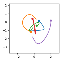
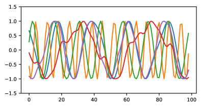
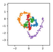
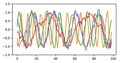
For both datasets, we generate 50,000 training and 10,000 validation samples. We restrict the number of test samples to 200, since the previous methods we compare to must be refit for each individual sample. We simulate systems with time-series. Our training and validation samples consist of time-steps, while the test-samples are time-steps long. This increased length allows us to infer causal relations on the first half of the data, and to test the future prediction performance on the second half (with ). In Figure 8, we show some examples of both the particles and Kuramoto datasets in the noiseless setting and with added noise.
Netsim
The Netsim dataset simulates blood-oxygen-level-dependent (BOLD) imaging data across different regions within the human brain and is described in Smith et al. (2011). The task is to infer the directed connections, i.e. causal relations, between different brain areas.
The Netsim dataset includes simulations with different numbers of brain regions and different underlying connectivity matrices. In our experiments, we use the data from the third simulation Sim-3.mat as provided by Khanna and Tan (2019). It consists of samples from 50 subjects, each with the same underlying causal graph, each of length and including different brain regions. Note, that we report worse results than Khanna and Tan (2019), since we assume self-connectivity for all time-series and only evaluate the causal discovery performance between different time-series.
The dataset is very small (50 samples) and due to this, we do not use a training/validation/test split, but use the same 50 points at each phase instead. While this is not standard machine learning practice, it still facilitates a fair comparison to the other methods, each of which is fit to individual test points. The purpose of including experiments on this dataset is not to demonstrate generalization ability, but rather to show that our method is flexible enough to work reasonably well even in the classical causal discovery setting (with one shared causal graph, and fitting the model on the test set).
B.1.2 Architecture and Hyperparameters
Our model is implemented in PyTorch (Paszke et al., 2019). We did no hyperparameter optimization for model training, but used the settings as described for the NRI model (Kipf et al., 2018). The latent dimension throughout the model is set to size 256. We optimize our model using ADAM (Kingma and Ba, 2015) with a learning rate of 0.0005. In the experiments on the particles dataset, the learning rate is decayed by a factor of 0.5 every 200 epochs. We set our batch-size to 128 and train for 500 epochs. The temperature of the Gumbel-Softmax is set to . During testing, this concrete distribution is replaced by a categorical distribution to obtain discrete edge predictions.
There was no thorough hyperparameter optimization done for test-time adaptation (TTA). Since there was no pre-existing implementation, some hand-tuning was performed. We use a learning rate of 0.1 for the Kuramoto and particles datasets and 0.01 for Netsim. For each, we run 1000 iterations.
Encoder
In our experiments, the amortized encoder applies a graph neural network on the input. It implements two edge-propagation steps along the causal graph:
| (15) | ||||
| (16) | ||||
| (17) | ||||
| (18) |
and are fully-connected networks (MLPs). On both the particles dataset and Netsim, is an MLP as well (MLP Encoder); on the Kuramoto dataset, we use a 1D CNN with attentive pooling (Lin et al., 2017) instead (CNN Encoder).
When conducting test-time adaptation as described in Eq. 7, we remove the encoder and model a distribution over using a non-amortized variational distribution with its initial values sampled from a unit Gaussian.
Decoder
The decoder implements a single edge-propagation step according to equations 12-14. It uses MLPs for both and . To improve performance, we train the decoder to predict several time-steps into the future. For this, we replace the true input with the predicted for steps.
Following our causal formulation of the NRI model, we implement Eq. 12 by masking out the values of the corresponding edges. Thus, the ordering of the edge types is not arbitrary in our setting.
We note that while this implementation of the decoder assumes a full-time graph of Markov order 1, the full ACD framework does not, and could be implemented using a recurrent architecture to remove this assumption.
Since our physics simulations are differentiable, we can replace the decoder with the ground-truth dynamics and backpropagate through them. We call this setup the simulation decoder.
Variance
When we report the variance on the ACD results, we collected these across five different random seeds. Baselines in Kuramoto/Netsim use three seeds each, except for NGC, which uses only one due to a longer runtime (the confidence intervals shown for NGC are confidence intervals on the AUROC itself, whereas all other confidence intervals are based on variance of AUROC across seeds).
B.1.3 Baselines
We compare ACD against several baselines:
Neural Granger Causality
From Tank et al. (2018), we optimized an MLP or LSTM to do next step prediction on a sample. We found that the MLP worked best. The causal links are wherever an input weight is non-zero. We used ADAM and then line search to find exact zeros. In this method, we calculate AUROC by running with a range of sparsity hyperparameters ( for Kuramoto and for Netsim). As in Tank et al. (2018), we calculate a score for each edge, where , and use that score to calculate AUROC. Code was used from https://github.com/icc2115/Neural-GC.
ESRU
Khanna and Tan (2019) take a similar approach to Tank et al. (2018), but they use economy statistical recurrent units (eSRU), instead of LSTMs. We found one layer worked best, and used their hyperparameters otherwise. We use sparsity hyperparameters for Kuramoto, and for Netsim. Code was used from https://github.com/sakhanna/SRU_for_GCI.
MPIR
Wu et al. (2020) determine where causal links exist by examining the predictive performance change when noise is added to an input variable. Code for this method and the baselines below was used from https://github.com/tailintalent/causal.
Transfer Entropy
Mutual Information
Using the implementation by Wu et al. (2020), we calculate the mutual information between every pair of time series.
Linear Granger Causality
Using the implementation by Wu et al. (2020), this is a linear version of Granger causality where non-zero linear weights are taken as greater causal importance.
We did not run the baselines on the particles dataset since it is two-dimensional and most baselines did not provide an obvious way for handling multi-dimensional time series. When training ACD on the particles and Kuramoto datasets, we additionally input the velocity (and phase for Kuramoto) of the time-series. Since our chosen NRI encoders and decoders are not recurrent we cannot recover this information in any other way in this model. This enables a more fair comparison to the recurrent methods, which are able to aggregate this information over several time steps.
B.2 Additional Experimental Result - Training Curves
Fig. 9 shows the training curves when training on 100 training samples of the particles dataset. We observe that the encoder overfits on the training samples, as indicated by the AUROC performance. In contrast, the decoder shows less overfitting as indicated by the negative log-likelihood (NLL) performance.
Appendix C Amortized Causal Discovery with Unobserved Variables
C.1 Temperature Experiments
Implementation Details
In this experiment, we use the CNN encoder and a simulation decoder matching the true generative ODE process. Our optimization scheme is the same as before.
For modeling the latent temperature, we output a uniform distribution as our posterior . One tricky aspect about this is the KL-Divergence:
| (19) |
We must ensure that our posterior support is a subset of our prior support. Otherwise, the KL-Divergence is undefined and optimization impossible. Recall that our prior is a uniform distribution over .
We output two latent parameters for each input and use these values to parametrize a mean and a half-width for the uniform distribution. First, we bound these values to represent a uniform distribution in . To achieve this, we let and with . We then sample a temperature , which is guaranteed to be bounded within . Stopping gradients, we use this temperature sample in the encoder to improve the causal discovery performance.
Next, we scale this result to the desired interval . To achieve this, we feed the scaled temperature into the decoder, and use the scaled distribution to find our KL term. We allow gradients to flow through the temperature sample in both the decoder and the distribution in the KL term, which informs our parameter updates.
Additional Results
Similarly to Fig. 6, we show the future prediction performance in MSE across different values of in Fig. 11. Again we find a slight improvement in performance when using ACD with Latent compared to the baselines, although this is a noisier indicator.
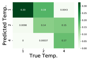
Additionally, we evaluate how well the introduced latent variable learns to predict the unobserved temperature. To do so, we use the mean of the predicted posterior uniform distribution. When a discrete categorical prediction is needed for evaluation, we quantize our results into three bins based on their distance in log-space. To calculate AUROC in this three category ordinal problem, we average the AUROC between the two binary problems: category 1 vs not category 1, and category 3 vs not category 3 (category 2 vs not 2 is not a valid regression task for the purposes of AUROC which is concerned with ordering, since it is the middle temperature and hence the labels would not be linearly separable).
The confusion matrix between true and predicted temperature in Fig. 11 indicates that ACD with Latent’s prediction tends to be conservative: it is more likely to predict a too low temperature than a too high one. This is probably due to higher temperatures incurring larger MSEs, since higher temperature systems are more chaotic and thus less predictable.
Table 3 lists the temperature prediction results across all tested values of . We find that we can predict the unobserved temperature quite well, especially with respect to ordering (as measured by correlation and AUROC).
[0.45]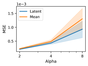 \ffigbox[0.45]
| 2 | 4 | 8 | |
| Correlation | 0.888 | 0.844 | 0.661 |
| Accuracy | 0.644 | 0.384 | 0.346 |
| AUROC (1vAll) | 0.966 | 0.935 | 0.843 |
C.2 Unobserved Time-series
Implementation Details
For modeling the unobserved time-series, we employ a two-layered, bi-directional long short-term memory (LSTM) (Hochreiter and Schmidhuber, 1997) with a latent dimension of size 256.
Additional Results
The full evaluation of our experiments with an unobserved time-series can be found in Table 4. Our results indicate that our proposed method ACD with latent predicts the trajectory of the unobserved time-series (unobserved MSE) more accurately than the Mean imputation baseline. Even though this prediction is worse than for the Supervised baseline, ACD with Latent manages to recover the performance of the fully Observed baseline better than the None and the Mean imputation baselines.
| Method | AUROC | Accuracy | MSE | unobserved MSE |
| Observed | (0.99) | (0.993) | (0.00301) | - |
| Supervised | 0.982 | 0.931 | 0.00822 | 0.0164 |
| None | 0.946 | 0.882 | 0.0119 | - |
| Mean | 0.951 | 0.881 | 0.0106 | 0.0397 |
| ACD with latent | 0.979 | 0.918 | 0.00747 | 0.0375 |
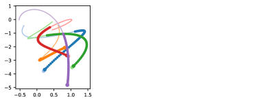
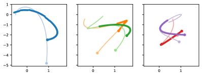
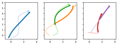
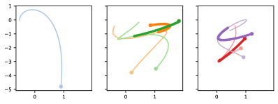
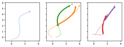
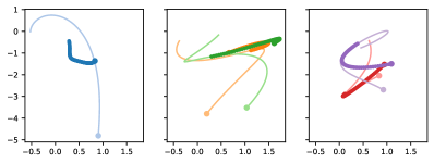
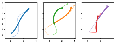
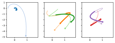
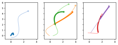
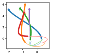
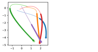
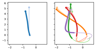
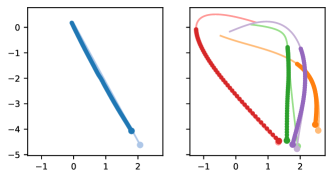
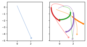
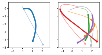
Fig. 12 shows the performance of the tested methods dependent on the number of time-series that are influenced by the unobserved one. In addition to Fig. 6 in our Experiments section, these plots show the achieved accuracy and MSE results. The general trends are the same. Fig. 13 shows example trajectories and the corresponding predictions for all tested methods.
Observed
Supervised
None
Mean
Latent
Additional Experiment: Uninfluenced Influencer
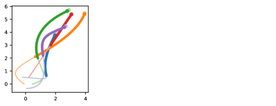
Predicting the trajectory of a time-series that influences only a small number of observed time-series and is (invisibly) influenced by them is arguably very difficult. In this follow-up experiment, we reduce the difficulty of this problem by adding two assumptions: (1) the unobserved time-series influences all observed time-series and (2) it is not influenced by any of the observed time-series. This way, we gain more information about its trajectory (due to (1)) and its trajectory becomes easier to predict (due to (2)). Indeed, in this setup, ACD with latent manages to almost completely recover the performance of the fully observed baseline (Table 5). In contrast, the performance of the None and Mean imputation baselines worsens considerably in this setting. Now, all time-series are influenced by the unobserved particle – making their prediction harder when not taking into account this hidden confounder. Fig. 14 shows example trajectories and the corresponding predictions for all tested methods in this setting.
| Method | AUROC | Acuracy | MSE | unobserved MSE |
| Observed | (1.0) | (0.997) | (0.0193) | - |
| Supervised | 1.0 | 0.993 | 0.024 | 0.000615 |
| None | 0.829 | 0.76 | 0.0431 | - |
| Mean | 0.853 | 0.782 | 0.0365 | 0.0357 |
| ACD with latent | 1.0 | 0.994 | 0.0251 | 0.137 |
Observed
Supervised
None
Mean
Latent
