MNRAS LaTeX 2ε template – title goes here

The relative orientation between the magnetic field and gradients of surface brightness within thin velocity slices of ¹²CO and ¹³CO emission from the Taurus molecular cloud

Abstract

We examine the role of the interstellar magnetic field to modulate the orientation of turbulent flows within the Taurus molecular cloud using spatial gradients of thin velocity slices of ¹²CO and ¹³CO antenna temperatures. Our analysis accounts for the random errors of the gradients that arise from the thermal noise of the spectra. The orientations of the vectors normal to the antenna temperature gradient vectors are compared to the magnetic field orientations that are calculated from Planck 353 GHz polarization data. These relative orientations are parameterized with the projected Rayleigh statistic and mean resultant vector. For ¹²CO, 28% and 39% of the cloud area exhibit strongly parallel or strongly perpendicular relative orientations respectively. For the lower opacity ¹³CO emission, strongly parallel and strongly perpendicular orientations are found in 7% and 43% of the cloud area respectively. For both isotopologues, strongly parallel or perpendicular alignments are restricted to localized regions with low levels of turbulence. If the relative orientations serve as an observational proxy to the Alfvénic Mach number then our results imply local variations of the Alfvénic Mach number throughout the cloud.

1 Introduction

Clouds of fully molecular gas within the Milky Way and nearby galaxies are characterized by internal non-thermal motions with speeds larger than the thermal sound speed of H₂. These supersonic motions are generally attributed to chaotic turbulent flows within the clouds and their surrounding environments that are driven by varying mechanisms at both small and large spatial scales (Larson, 1981). If the interstellar magnetic field that threads through the clouds is sufficiently strong and the collisional time scale between ions and neutral molecules is short with respect to an Alfvén wave crossing time, then the character of the turbulent flows is necessarily modified (Mouschovias et al., 2011). In these conditions, both energy and momentum can be redistributed by Alfvén waves whose amplitudes are largest when the wave vectors are parallel (transverse) or perpendicular (magnetosonic) to the local magnetic field direction. The action of such waves introduces anisotropies in the distribution and motions of the gas (Arons & Max, 1975; Mouschovias et al., 2011).

Detailed predictions of anisotropy have emerged from theories of interstellar MHD turbulence. Goldreich & Sridhar (1995) (hereafter, GS95) examined the effects of the interaction between oppositely-directed packets of shear Alfvén waves on a magnetized fluid. In the limit of strong Alfvénic turbulence, they showed that turbulent eddies become elongated along the magnetic field direction and that the wave vectors parallel and perpendicular to the local magnetic field direction scale as k${}_{\parallel}\propto k_{\perp}^{2/3}$. Goldreich & Sridhar (1997) extended this study to an intermediate turbulence regime and considered the effects of pseudo Alfvén waves that correspond to slow magnetosonic waves in the incompressible limit. They demonstrated that the pseudo Alfvén waves (hereafter slow mode) exhibit the same velocity spectrum and anisotropy as the shear Alfvén modes.

The anisotropy considered in GS95 was in relation to the mean magnetic field. In fact, the anisotropic eddies are aligned with the direction of the local magnetic field on the scale of the eddy. The increasing elongation of eddies with decreasing scale in the local frame of reference was affirmed by Lazarian & Vishniac (1999) (LV99) who considered the effects of magnetic reconnection on the gas motions and field structure. LV99 showed that, in the presence of turbulence, the altered magnetic field line topology is a natural consequence of the turbulent cascade while, at the same time, reconnection itself can further drive turbulence. As the turbulent cascade proceeds perpendicular to the magnetic field, reconnection becomes fast, with reconnection taking place on order of the local eddy turnover time. The result of fast reconnection is that the velocity fluctuations will be aligned with the local field, a result which has major implications for many astrophysical processes such as cosmic ray diffusion, star formation and ISM structure. Using MHD simulations of compressible gas, Cho & Lazarian (2003) further verified velocity anisotropy imposed by the magnetic field in the local frame of reference for both Alfven and slow modes in the regime where the ratio of thermal to magnetic field energy densities is $<<$1.

In addition to the MHD waves, magnetically-induced velocity anisotropies can also emerge from the large scale flows in a compressible medium. For a strong magnetic field, the MHD equations predict a binary state in which gas motions are either along or perpendicular to the magnetic field (Soler & Hennebelle, 2017). Furthermore, collapse of material along field lines can lead to hydrodynamic shocks and anisotropic density distributions (Chen & Ostriker, 2015; Mocz & Burkhart, 2018).

Can such magnetically-induced velocity anisotropy be measured in the molecular interstellar medium? The study of Cho & Lazarian (2003) provides a valuable basis on which to build a framework of analyses that can identify such conditions. In their set of MHD simulations, they show iso-contours of the two-dimensional structure function of velocities with respect to the local magnetic field direction. As the structure function quantifies the degree of velocity correlation along 2 orthogonal axes, its shape and orientation represents the spatial configuration of the turbulent eddies in the reference frame of the local field.

Esquivel & Lazarian (2005) and later, Esquivel & Lazarian (2011) and Burkhart et al. (2014) examined shapes and elongations of the two-dimensional structure functions of density-weighted velocities from a set of MHD simulations spanning a large range in both Alfvén and sonic Mach numbers. These studies found alignment of elongated structure functions and hence, turbulent eddies, with the projected, perpendicular component of the magnetic field along the line of sight. This alignment held for models with sub-Alfvénic motions and sonic Mach numbers as high as 7. Esquivel et al. (2015) extended this analysis to line intensities of position-position-velocity data derived from MHD simulations for varying magnetization and spectral resolutions. For high spectral resolution slices of the data cube, they found elongated structure functions with long axes aligned with the orientation of the magnetic field for strongly magnetized models.

Heyer et al. (2008) applied Principal Component Analysis (PCA) to position-velocity slices of spectroscopic data cubes to evaluate the velocity structure function along orthogonal axes. Using model CO line profiles derived from density and velocity fields of MHD simulations, they also found the orientation of velocity anisotropy to be aligned with the local magnetic field direction but only for sub-Alfvénic models. Applying this method to a localized area in the Taurus molecular cloud with striations of CO emission oriented along the magnetic field, they found the strongest anisotropy of the velocity structure functions is also aligned with the magnetic field. A followup study by Heyer & Brunt (2012) over a mosaic of fields in the Taurus cloud showed that velocity anisotopies are limited to low column density regions of the cloud. They suggested that a transition from sub-Alfvénic conditions in the low column density envelope of the cloud to super-Alfvénic motions in the high density cloud interior to account for the different behavior.

While structure function methods and PCA offered initial clues to MHD anisotropy, both these analyses are limited to analyzing sufficiently large areas within a cloud to accurately evaluate the velocity structure function along each axis. Therefore, these methods are insensitive to small scale anisotropies that are predicted by theories of MHD turbulence.

More recently, the orientation of spatial gradients of column densities and velocity centroids with respect to that of the magnetic field has been an effective tool to investigate MHD turbulence. Soler et al. (2013) found a bimodal distribution of relative orientations of column density gradient vectors and magnetic field orientations on a set of numerical simulations with varying magnetization. For low density regions within the simulations and higher magnetizations, the angles of the vectors normal to the gradient vectors are aligned with the local magnetic field. For higher density regions, the normal vectors are perpendicular to the magnetic field orientations. This bimodal effect is also present in a set of local clouds observed by the Planck mission, which provides both dust column density and dust polarization (Planck Collaboration Int. XXXV, 2016). González-Casanova & Lazarian (2017) extended this analysis to gradients of velocity centroids of spectral line emission (VCG) that can be more directly compared to the kinematics of MHD turbulence.

These applications of the gradient techique analyzed either direct two-dimensional images of clouds such as column density or projections of spectroscopic data cubes of line emission such as moment maps. However, there is much more information within the full data cubes of spectral line emission that can be exploited. Lazarian & Yuen (2018a) adapted the gradient method to spectral line intensities within thin velocity slices of the data cube (Velocity channel gradients, VChG). For very thin spectral channels, the structure of line emission is most affected by the velocity field of the volume rather than the distribution of gas densities (Lazarian & Pogosyan, 2000; Brunt & Mac Low, 2004). The advantage of this analysis over previous methods is its ability to define a vector that describes the magnitude and direction of line intensity differences that arise from the turbulent flow of gas, gravity, or feedback processes from newborn stars at the resolution of the observations.

Hu et al. (2019) applied the VChG method to optically thin, molecular line emission from several nearby molecular clouds including the Taurus ¹³CO data analyzed in this study. They found good alignment of the magnetic field orientation with that of the vector normal to the velocity centroid gradient vector. From the width of the distributions of either gradient angles or polarization orientations ($\delta\theta$) and applying the Davis-Chandrasekhar-Fermi relation M_A = tan($\delta\theta$) (Davis & Greenstein, 1951; Chandrasekhar & Fermi, 1953), they estimated Alfvén Mach numbers in these clouds between 0.7 to 1.2.

In this contribution, we examine the orientations of gradients of ¹²CO and ¹³CO intensities within a large set of narrow velocity channels with respect to magnetic field orientations as measured by Planck (Planck Collaboration Int. XIX, 2015) for the Taurus molecular cloud. Analysis of both optically thick ¹²CO emission and mostly optically thin ¹³CO emission may provide insight to the effects of line opacity on the on the VChG method. Our calculations of intensity gradients specifically include the effects of thermal noise of the spectral line data and the impact of the resultant gradient angle uncertainties on circular statistics used to parameterize the degree of orientation alignment. In §2, we summarize our data. Our assumptions and analysis methods are described in §3. The results of the analysis are shown in §4. In §5, we examine the dependence of the degree of relative orientations with the local gas properties. The interpretation of these results are described in §6.

2 Data

2.1 ¹²CO and ¹³CO J=1-0 emission

All molecular line data used in this study are part of the FCRAO Survey of the Taurus molecular cloud described by Narayanan et al. (2008) and Goldsmith et al. (2008). The survey imaged ¹²CO and ¹³CO J=1-0 emission from 96 deg² of the Taurus cloud with the 14 meter telescope of the Five College Radio Astronomy Observatory using On-the-Fly (OTF) mapping. The front-end consisted of the 32-element focal plane array receiver, SEQUOIA, that fed a set of autocorrelation back end spectrometers configured with a spectral resolution of 25 kHz or 0.063 km s^-1 and 0.067 km s^-1 for ¹²CO and ¹³CO respectively. The half power beam widths for ¹²CO and ¹³CO are 45″ and 47″. The spacing between pixels in the final regridded map is 20″ for each transition.

2.2 Polarized thermal dust emission

We analyze the same Planck HIFI polarization data at 353 GHz that was used by Planck Collaboration Int. XXXV (2016) to map the magnetic field configuration in the Taurus cloud. We assume that the orientation of the plane-of-the-sky magnetic field is perpendicular to the orientation of the linear polarization at 353 GHz, that is, assuming perfect dust grain alignment, as justified by the results of Planck Collaboration et al. (2018). This data set, comprised of Stokes I, Q and U maps, is smoothed to 10′ to achieve polarization signal-to-noise ratios $P/\sigma(P)>$ 3. These maps are obtained using a gnomonic projection of the publicly-available whole-sky maps, available through the Planck Legacy Archive in Healpix format. The initial projection is made in Galactic coordinates and subsequently transformed into equatorial coordinates and aligned with the ¹²CO and ¹³CO maps using the reproject package in astropy and the corresponding rotation of Stokes $Q$ and $U$ to this reference frame using the polgal2equ included in the magnetar package .

The polarization orientation of the E-vector is calculated for each position in the reprojected $U$ and $Q$ images following the IAU convention in which positive angles are measured counterclockwise from the positive declination axis, such that,

$$\Psi_{E}(\alpha,\delta)=0.5\arctan{\biggl{(}\frac{-U(\alpha,\delta)}{Q(\alpha,\delta)}\biggr{)}}$$ (1)

where $\alpha,\delta$ are the equatorial coordinates and $\Psi_{E}$ is the polarization angle in equatorial coordinates. Assuming elongated dust grains that are responsible for the polarization are aligned with the magnetic field, $\Psi_{B}(\alpha,\delta)=\Psi_{E}-\pi/2$ is the orientation of the magnetic field component perpendicular to the plane of the sky.

2.3 Column Density derived from thermal dust emission

To evaluate column density, we use the same map of the 353 GHz opacity that was constructed from all-sky Planck intensity measurements at 353, 545, and 857 GHz and supplemented by IRAS observations at 100 µm and analyzed by Planck Collaboration XI (2014). The opacity was smoothed to 10′ resolution and converted into column density, $\tau_{353}/N_{H}=1.2{\times}10^{-26}$ cm², assuming a dust opacity based on extinction measurments towards quasars. The column density image was transformed into equatorial coordinates and similarly aligned with the CO data with the astropy reproject package.

2.4 Wide field views of molecular gas and magnetic field orientations in Taurus

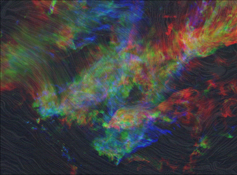
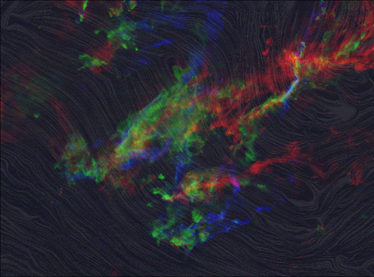
Figure 1: Velocity-encoded RGB images of ¹²CO (top) and ¹³CO (bottom) J=1-0 emission with a drapery pattern showing the magnetic field orientations from Planck 353 GHz polarization data. The colors represent CO emission integrated over $V_{{\rm LSR}}$ intervals: 3.7-5.5 km s^-1(blue), 5.5-6.3 km s^-1(green), and 6.3-7.8 km s^-1(red).

The wide field distribution of ¹²CO and ¹³CO J=1-0 emission within 3 velocity intervals and a representation of the magnetic field orientations derived from the Planck 353 GHz polarization data are displayed in Figure 1. The rgb colors represent the emission integrated over velocity intervals through which most of the cloud CO luminosity is radiated: 3.7-5.5 km s^-1(blue), 5.5-6.3 km s^-1(green), and 6.3-7.8 km s^-1(red). The magnetic field orientation is imprinted as localized folds of the CO intensity image as produced by the line integral convolution method (Cabral & Leedom, 1993).

The two CO images show very different intensity distributions. The ¹³CO image is similar to the Planck column density map and images of visual extinction (Pineda et al., 2010) in which most of the emission is distributed into filaments or localized clumps. In contrast, the ¹²CO image is more extended with flocculent features. These differences arise from the relative opacities of the two emission lines. The high opacity of ¹²CO for a given velocity interval limits the depth to which emission can probe. The high optical depth also maintains the excitation temperature by radiative trapping in regions where the volume density is much less than the critical density and allowing the ¹²CO line to be detected in this regime, which accounts for its more extended surface brightness distribution.

The magnetic field orientation varies smoothly across the cloud area. There are no abrupt changes in the field orientation when crossing from a low column density area into a high density filament. Visually, the magnetic field aligns with the faint, wispy striation features in the northeast sector of the CO maps. Towards the central region of the cloud, higher column density material is distributed perpendicular to the field orientation. Our goal in this investigation is to quantify these orientations in order to evaluate the more general alignment of the interstellar magnetic field and the gas distribution.

3 Assumptions and Analysis

3.1 Thin-Slice intensity images

Spectroscopic imaging of low J ¹²CO and ¹³CO line emission exhibits very complex structure that results from both density variations and a turbulent velocity field. Lazarian & Pogosyan (2000) examined the impact of density and velocity on the power spectrum of 2-dimensional channel images of spectroscopic data cubes, $T(x,y,v)$ with varying velocity slice thickness. In the regime for which the velocity width of the slice, ${\Delta}v$ is greater than the velocity dispersion, $\sigma_{v}(L)$ over size $L$, the power spectrum of intensity fluctuations of an optically thin line reflect column density variations. Conversely, for ${\Delta}v<<\sigma_{v}(L)$, corresponding to the thin-slice limit, the power spectrum of an image of brightness temperatures is dominated by velocity variations. Velocity Channel Analysis (VCA) developed by Lazarian & Pogosyan (2000) is a procedure to separate the dependence of the power spectrum on column density and velocity fluctuations using both thick and thin slice channel widths in order to derive the functional form of the power spectrum for both column density and velocity fields. In this study, we assume that structure in the thin slice channels reflect caustics of the turbulent velocity field rather than density fluctuations of a turbulent cell. This is a reasonable assumption for cold, molecular gas where the linewidth is dominated by turbulent broadening rather than thermal broadening (Clark et al., 2019).

3.2 Gradients of surface brightness in thin-slice velocity channels

Spatial gradients of spectral line intensities, column densities, or centroid velocities are powerful measures of cloud structure and anisotropies. The gradient calculation produces a vector at each sampled position, (x,y), that describes the magnitude and direction of localized differences of field values. In this study, we investigate the spatial gradients of brightness temperature of ¹²CO and ¹³CO J=1-0 line emission in thin slice channels. For notation, we define the $k$-th velocity slice of the data cube of brightness temperatures $T(x,y,v_{k})$ as $T_{k}(x,y)$. The gradient magnitude and direction for this $k$-th slice are

$$\nabla{\rm T_{k}(x,y)}=\bigg{\{}\bigg{(}\frac{\partial{{\rm T_{k}(x,y)}}}{\partial{{\rm x}}}\bigg{)}^{2}+\bigg{(}\frac{\partial{{\rm T_{k}(x,y)}}}{\partial{{\rm y}}}\bigg{)}^{2}\bigg{\}}^{1/2}$$ (2)

$$\Psi_{G,k}=\arctan\left[\frac{\partial T_{k}(x,y)}{\partial x}\middle/\frac{\partial T_{k}(x,y)}{\partial y}\right]$$ (3)

where $\Psi_{G,k}$ is the direction of the gradient measured counter-clockwise from the $y$ (declination) axis. Here, we calculate the angle of the vector normal to the gradient vector, $\Psi_{N,k}=\Psi_{G,k}+\pi/2$, which describes the orientation of the longer axis of an emission feature that is responsible for the gradient. Following Soler et al. (2019), the multi-dimensional filter routine, gaussian_filter, in the python scipy.filters package is applied to the image. This filter includes a smoothing option that both increases the signal to noise of the gradient measurement and sets an angular scale over which the gradient is derived, which corresponds to the Gaussian derivatives introduced by Soler et al. (2013). For the Taurus CO data, a Gaussian kernel with a full width half maximum of 8 pixels (2.67 ′ $\approx$ 1/4 Planck Stokes $U$ and $Q$ FWHM angular resolution) is applied to derive the gradient vectors.

Random noise can have a significant effect on the gradient calculation so it is important to track how noise in the data impacts the accuracy of the gradient magnitude and gradient angle. We adopt a Monte Carlo approach to assess these errors. Derivatives of the thin-slice intensity images are calculated from $T_{k}(x,y)=T_{obs,k}(x,y)+T_{noise,k}(x,y)$, where $T_{obs,k}(x,y)$ is the observed antenna temperature at the position $(x,y)$ and velocity slice k and $T_{noise,k}(x,y)$ is randomly drawn value from a gaussian probability density distribution with the same width as the rms uncertainty of the spectrum at position x,y. The gradient amplitude and angle are derived from equations 1 and 2 respectively. This is repeated for 1024 realizations producing distributions of the gradient amplitude and angle for each sampled position. The respective uncertainties are assigned to the standard deviation of each distribution for position (x,y).

3.3 Directional Statistics

The gradient analysis generates a set of angles that are compared to the magnetic field orientation in the vicinity of the measurements. We define $\Phi_{k}(x,y)=\Psi_{N,k}(x,y)-\Psi_{B}(x,y)$, where $\Psi_{B}(x,y)$ is the angle of orientation of the interstellar magnetic field component perpendicular to the plane of the sky at position (x,y) that is interpolated from the Planck data to the 2.67’ sampling interval. The set of $\Phi$ values is represented by the projected Rayleigh statistic,

$$Z_{k}=\frac{\sum_{i}w_{k}(x_{i},y_{i})\cos(2\Phi_{k}(x_{i},y_{i}))}{(\sum w_{k}(x_{i},y_{i})^{2})^{1/2}/2}$$ (4)

and its variance

$$\sigma(Z_{k})^{2}=\frac{2\sum_{i}(\cos(2\Phi_{k}(x_{i},y_{i}))^{2}-Z_{k}^{2}}{n_{ind}}$$ (5)

where the sums are over all sampled pixels in the area, $w_{k}(x_{i},y_{i})$ is a weighting factor for the i-th sampled position, and $n_{ind}$ is the number of independent measurements (Jow et al., 2018). It is evident that $Z_{k}>>0$ for strongly aligned features, $Z_{k}<<0$ for features orthogonally oriented, and $Z_{k}\sim 0$ for a set of random, uniformly distributed orientations. Such random, uniform distributions can arise from a field with just noise (no signal) or a field with signal and significant gradient orientations but are randomly distributed or a mixture of both conditions.

In calculating the projected Rayleigh statistic, it is necessary to evaluate the number of independent samples as oversampling a field can introduce a strong bias to the result. Fissel et al. (2019) proposed that the number of independent data samples in a field is

$$n_{ind}=\frac{n_{eval}}{\sigma(Z_{WN})^{2}}$$ (6)

where $n_{eval}$ is the number of evaluated pixels and $\sigma(Z_{WN})$ is the standard deviation of $Z_{k}$ values derived from a series of images filled with white noise (WN) that is smoothed and sampled identically to the data.

The point spread functions of the Planck 353 GHz $U$ and $Q$ images have a full width half maximum width of 10′. The gradient analysis requires one to sample at finer scales than the Planck beam size in order to detect small scale differences in the velocity slice images. In our study, the thin-slice channel images are smoothed to 2.67′ resolution as part of the gradient calculation. When deriving $\Phi_{N,k}$, we evaluate the gradient angle image at this same interval rather than the 20″ pixel spacing of the CO data. We calculate $\sigma(Z_{WN})$ using 2 independent methods. The first method follows the prescription of Fissel et al. (2019) in which an image is populated with spatially uncorrelated, normally distributed random values with the same dispersion as the data. The image of $\Phi_{WN}$ values derived from white noise fluctuations is sampled identically to the Taurus data to derive the projected Rayleigh statistic and its variance. This is repeated for 1024 realizations to derive a mean $Z_{k}$ value and standard deviation, $\sigma(Z_{WN})$. The second method evaluates the projected Rayleigh statistic in velocity channels with no signal. This allows one to assess the impact of correlated noise in our data due to On-the-Fly mapping. Both methods produce $Z_{k}$ values near zero and $\sigma(Z_{k})\approx$ 1 as expected for a set of independent measurements. From these noise results, we conclude the oversampling introduced by the Planck beam, by a factor close to 16 in area, does not introduce a systemic bias in our derived values of $Z_{k}$ such that $n_{ind}=n_{eval}$ and no corrections are required.

4 Results

The Taurus molecular cloud presents a range of gas column densities and magnetic field orientations. To assess any dependency of the gas-field coupling on the local conditions, we partition the Taurus data into 150 subfields. Each subfield is comprised of 256$\times$256 pixels (1.42$\times$1.42 deg², which corresponds to physical dimensions 3.5$\times$3.5 pc²). The subfields are spaced by 128 pixels in each direction. This partitioning is identical to that applied by Heyer & Brunt (2012). In §8.3, we describe the effects of decreasing the subfield sizes to 128$\times$128 pixels and 64$\times$64 pixels.

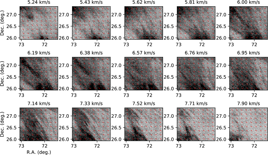
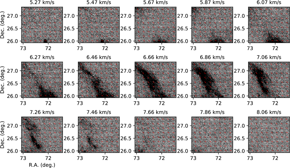
Figure 2: A set of thin-slice velocity channel images of ¹²CO (top) and ¹³CO (bottom) J=1-0 emission from 1 subfield area (1.42$\times$1.42 deg²) in the vicinity of magnetically aligned striations in the Taurus molecular clouds (Goldsmith et al., 2008; Heyer et al., 2016). The red segments represent the orientation of the magnetic field derived from 353 GHz Planck polarization data with 10′ resolution but displayed every 5.3′. The halftone of ¹²CO emission ranges from $-$1 to 2.5 K for each image. For ¹³CO emission, the halftone ranges from $-$0.5 to 0.5 K.

Figure 2 shows a mosaic of 15 thin-slice channel images of ¹²CO and ¹³CO J=1-0 emission from a subfield in the Taurus molecular cloud between $V_{{\rm LSR}}$ 5.24 and 8.06 km s^-1. To increase the signal to noise for each velocity slice image, the data are smoothed over 3 spectral channels providing a slice thickness of 0.19 km s^-1 for ¹²CO and 0.2 km s^-1 for ¹³CO. This velocity slice width is still smaller than the typical velocity dispersion of $\sim$1 km s^-1  over the subfield size and therefore, within the thin-slice limit. The red segments represent the orientations of the magnetic field component perpendicular to the plane of the sky derived from the Planck 353 GHz polarization data. This particular field is the area noted by Goldsmith et al. (2008) that exhibits emission striations and strong velocity anisotropy that is aligned with the magnetic field orientation (Heyer et al., 2008; Heyer & Brunt, 2012; Heyer et al., 2016). Therefore, it offers a best-case example of velocity anisotropy. The emission from both isotopologues is weak (T_mb $<$ 2 K) as this subfield is located in the periphery of the cloud that is well displaced from the high column density regions with active star formation. The CO emission is stretched-out along the magnetic field orientation in many of these channel images. Neighboring subfields exhibit similar alignment of the emission over these intervals.

4.1 Histogram of oriented gradients from the Taurus molecular data

The gradient analysis is applied to the set of ¹²CO and ¹³CO velocity slices between the V_LSR interval -5 and 15 km s^-1 for each subfield. Most of the signal from the Taurus cloud emits within $V_{{\rm LSR}}$ interval 4 to 8.5 km s^-1. The broader interval ensures sufficient baseline coverage to compile statistics of random noise. Figure 3 displays the image of gradient amplitudes derived from each velocity slice image shown in Figure 2. The cyan colored segments show those vectors with gradients that are greater than 4 K/pc (¹²CO) and 2.2 K/pc (¹³CO). These gradient thresholds are based on where the median error of the gradient angle is less than 15^∘ (see Figure 11), and are only used to highlight the most statistically significant gradients. The red segments represent $\Psi_{B}$. The gradient features in Figure 3 typically persist for several contiguous channels (0.6 km s^-1). Many of the gradients in this field are aligned with the near uniform magnetic field orientations. This alignment is particularly strong in channel images between 6.9 and 7.5 km s^-1.

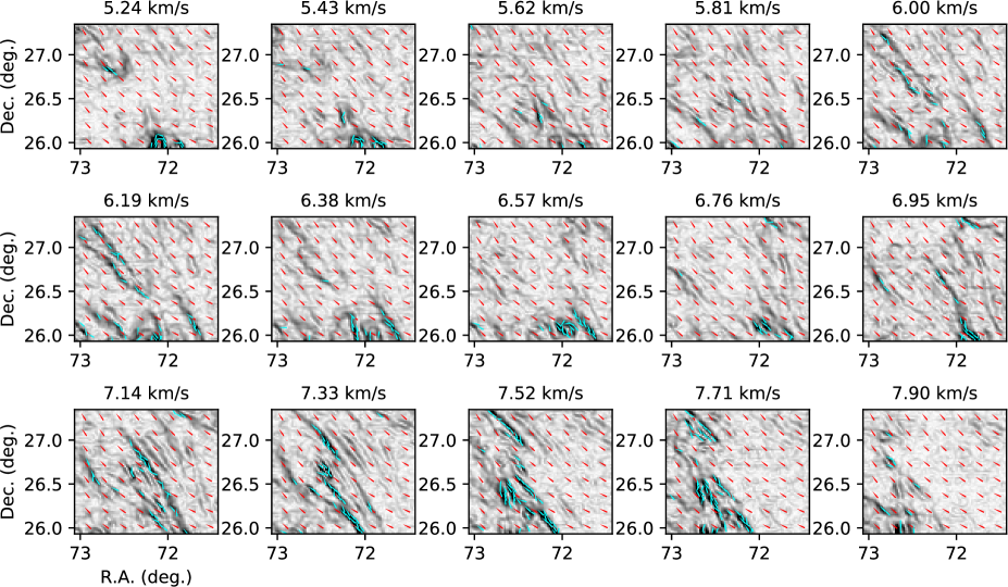
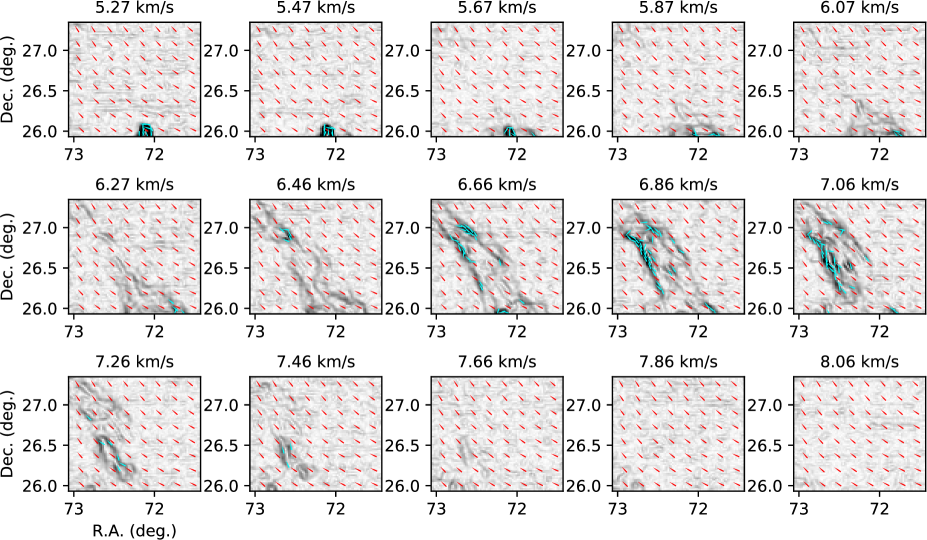
Figure 3: Images of gradient vector magnitudes of velocity slice images shown in Figure 2. The halftone ranges from 0 to 8 km s^-1 pc^-1 for ¹²CO and 0 to 4 km s^-1 pc^-1 for ¹³CO. The red segments show the orientation of the magnetic field component in the plane of the sky. The cyan segments show the orientation of the gradient normal. Only segments with $|{\nabla}T(x,y,v_{i})|>$ 4 K pc^-1 for ¹²CO and $|{\nabla}T(x,y,v_{i})|>$ 2.2 K pc^-1 for ¹³CO are shown for clarity.

The degree of alignment is further illustrated in Figure 4, which shows histograms of the differences between the position angles of the gradient normal vector and the Planck-derived magnetic field orientations for each channel image in this demonstration field. The light grey histograms show the distributions of $\Phi_{k}$ values for all sampled pixels in each image while the cyan histograms show the $\Phi_{k}$ distribution for sampled pixels with ${\nabla}I>$ 4 K pc^-1 for ¹²CO and ${\nabla}I>$ 2.2 K pc^-1 for ¹³CO, for which the gradient angles are more reliably determined with respect to random noise effects. There are many positions in the field for a given velocity slice for which there is weak or no detected line emission. The gradient angles from these pixels are random and produce a mostly flat $\Phi_{k}$ distribution. The cyan colored distributions in velocity channels 6.95 to 7.52 km s^-1 are not precisely centered on zero degrees but show that the majority of pixels with well defined gradients have $|\Phi_{k}|$ values less than 20^∘. These confirm the alignment that is visually evident in Figure 3.

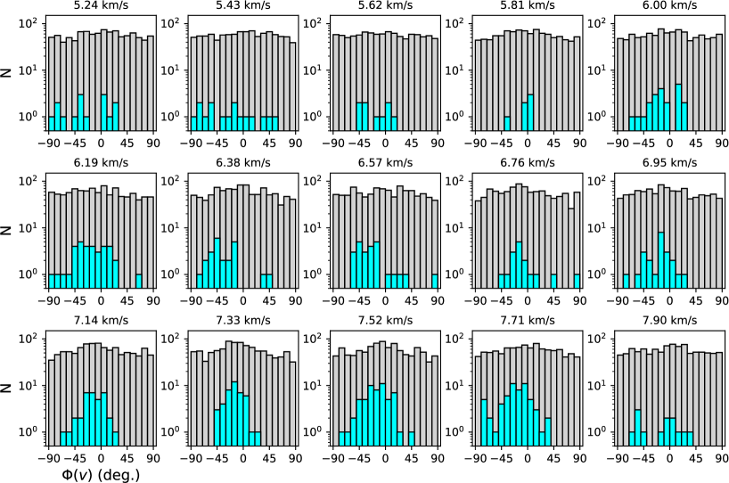
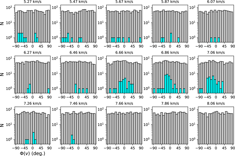
Figure 4: Histograms of the relative orientation between the gradient normal vector and the magnetic field orientation for each thin-slice field shown in Figure 2. The light-grey shading shows the distribution of $\Phi$ values for all sampled pixels while the cyan histogram shows the distribution of $\Phi$ values for pixels with ${\nabla}I>$ 4 K pc^-1 (¹²CO) and 2.2 K pc^-1 (¹³CO).

The projected Rayleigh statistic, $Z_{k}$, described in §3.3 offers a more quantitative assessment of the degree of alignment for a set of relative orientations than visual inspections of histograms. The variations of $Z_{k}$ values for each computed velocity slice for the demonstration field for both ¹²CO and ¹³CO are presented in Figure 5. In calculating $Z_{k}$ for a given image, all sampled pixels are used but are weighted by the factor $1/\sigma(\Phi_{k})^{2}$, where $\sigma(\Phi_{k})$ is the random error in $\Phi_{k}$ values derived for each sampled pixel as estimated from the Monte Carlo calculation of $\Psi_{N,k}$ as well as uncertainties of $U$ and $Q$ values. Examining Figure 5, it is useful to first inspect values in the velocity intervals with no emission. For this field, these intervals are [-5,+2] km s^-1 and [10,15] km s^-1. Ideally, the random noise in these images should generate $Z_{k}$ values near zero. The small but visible bias of $Z_{k}$ towards small negative values is likely a result of spatially correlated noise of the spectral line data that arises from OTF mapping. As already described, the standard deviation of $Z_{k}$ values in these intervals is $\sim$1. For this field, most of the emission occurs within the velocity interval [4.5,9] km s^-1(see Figure 1). Within this interval, the $Z_{k}$ values are positive and often greater than 3 corresponding to signal to noise greater than 3 and indicative of mostly parallal alignments. The largest $Z_{k}$ values occur within channels that are slightly red-shifted with respect to the mean velocity of this subfield – a feature previously noted by Heyer et al. (2016) in this field.

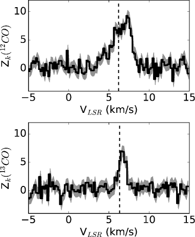
Figure 5: The variation of the projected Rayleigh statistic, $Z_{k}$ with $V_{{\rm LSR}}$ for the demonstration subfield shown in Figure 2 for ¹²CO (top) and ¹³CO (bottom). The light-grey shading shows the 1-$\sigma$ error in $Z_{k}$ values derived from Monte Carlo realizations. The vertical dashed line in each plot shows the mean velocity of the subfield field for each isotopologue. For both ¹²CO and ¹³CO, the subfield shows statistically significant alignment of thin-slice intensity gradients with the magnetic field orientation in narrow velocity intervals.

4.2 All sub-fields

Figures 2-5 provide a demonstration of the gradient analysis for a single subfield. We have applied this method to all 150 subfields to assess the degree of gradient alignment throughout the Taurus cloud and its dependence on local gas properties. Previous studies have shown that the magnetic field orientations derived from the Planck polarization data vary smoothly across the Taurus cloud (Planck Collaboration Int. XXXV, 2016; Hu et al., 2019). At 353 GHz, the thermal dust emission is optically thin so these orientations should represent the density weighted average of the magnetic field orientation along the line of sight. However, we caution that this projected magnetic field orientation may not reflect the 3-dimensional topology of the magnetic field within the gas layers traced by each thin velocity slice. Any decoupling of gas layers respectively traced by the polarization and thin-slice line emission would introduce increased variance in the distribution of $\Phi_{k}$.

Figure 6 shows images of $Z_{k}$ values derived from the ¹²CO and ¹³CO data for a subset of all analyzed velocity slices. Each pixel in these maps represents the $Z_{k}$ value for each subfield. The color lookup table is diverging in order to identify subfields with thin-slice intensity gradients that are strongly aligned (red), perpendicular (blue), or random (white). The overlayed contours show the distribution of hydrogen column density from the Planck data but sampled at the resolution of each subfield (1.42^∘ or 3.5 pc). The 1$\sigma$ uncertainty in $Z_{k}$ values is $\sim$1 so only the strongly red or blue colors denote significant alignment (parallel or perpendicular). In both the ¹²CO and ¹³CO data, the northeast region of the cloud exhibits the largest positive $Z_{k}$ values over the interval 5.75 to 7.75 km s^-1. These striation features are elongated along the local magnetic field direction. For the high column density regions, which typically correspond to dense filaments in both dust continuum and ¹³CO line emissions, $Z_{k}$ values are mostly negative over the velocity range 5 to 7 km s^-1. These negative values are a result of the edges of the filaments, which generate large gradients, whose normal orientations are perpendicular to the local magnetic field.

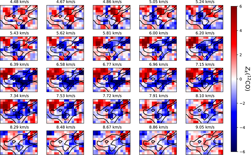
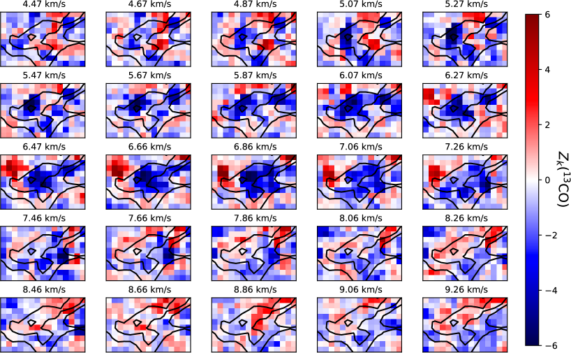
Figure 6: Images of the projected Rayleigh statisitic, $Z_{k}$, for ¹²CO (top) and ¹³CO (bottom) calculated over each subfield of the Taurus molecular cloud. Axis labels are not shown for clarity but would be identical to those in Figure 7. The contours represent the log of the hydrogen column density (cm^-2) derived from Planck dust emission that has been resampled to the effective resolution of the $Z_{k}$ image. The contour levels are 21.5, 21.75, and 22. There is strong alignment of the velocity gradient normal vector position angle with the magnetic field orientation (red colors) in the northeast for most thin-slice images. In the highest column density regions, there is a strong signal of perpendicular relative orientation (blue colors) in the ¹³CO data that more accurately traces such regions relative to ¹²CO.

4.3 Projected Velocity integrated Rayleigh Statistic

Magnetically aligned anisotropies are evident in the gradient images over very narrow velocity intervals – typically less than 1 km s^-1(Heyer et al., 2016). Here, we address whether alignments are coherent over larger velocity intervals as inferred in Figure 5. The velocity-integrated Rayleigh statistic is

$$Z_{int}=\frac{\sum_{k}\sum_{i}w_{k}(x_{i},y_{i})\cos(2\Phi_{k}(x_{i},y_{i}))}{(\sum_{k}\sum_{i}w_{k}(x_{i},y_{i})^{2})^{1/2}/2}$$ (7)

where the sum i is over all sampled pixels in each subfield and the sum k is over all velocities within the interval 5 to 8 km s^-1. This velocity interval accounts for 69% and 83% of the ¹²CO and ¹³CO luminosities respectively. $Z_{int}$ is similar to the method of Hu et al. (2019), which analyzes the histogram of all thin-slice gradient orientations compiled over a larger velocity interval to derive the relative orientation of a subfield.

The projected velocity integrated Rayleigh statistic is complemented by the velocity-integrated mean resultant vector,

$$r_{int}=\frac{\Bigl{[}C^{2}+S^{2}\Bigr{]}^{1/2}}{\Bigl{(}\sum_{k}\sum_{i}w_{k}(x_{i},y_{i})\Bigr{)}}$$ (8)

where

$$C=\sum_{k}\sum_{i}w_{k}(x_{i},y_{i})\cos(2\Phi_{k}(x_{i},y_{i}))$$ (9)

$$S=\sum_{k}\sum_{i}w_{k}(x_{i},y_{i})\sin(2\Phi_{k}(x_{i},y_{i}))$$ (10)

The mean resultant vector is the quadrature sum of 2 terms: $C$ measures whether there is a preferred orientation with respect to 0 or 90 degrees; $S$ measures whether there is a preferred orientation with respect to 45 or 135 degrees. Unweighted, it is the fraction of gradient vectors pointing in a preferred direction but does not carry information on what that preferred direction is (Soler et al., 2019). Weighting the calculation by $1/\sigma(\Phi_{k}(x_{i},y_{i}))^{2}$, $r_{int}$ reflects this fraction biased towards pixels with small instrumental $\Phi$ errors and provides a normalized estimate of the significance of the alignment. The values of $Z_{int}$ and $r_{int}$ are used together to establish the degree of alignment between two orientations. The mean resultant vector also resolves the degeneracy of $Z$ for a set of random orientations for which $Z$=0 and $r$=0 and a set of orientations all at 45^∘ for which $Z$=0 and $r$=1.

Images of $Z_{int}$ and $r_{int}$ for ¹²CO and ¹³CO are shown in Figure 7. Submaps with higher values of $r_{int}$ have more reliable measures of $Z_{int}$ values. As shown in Figure 13 in the Appendix, values of $r_{int}>0.1$ correspond to $Z_{int}/\sigma(Z_{int})>3$. The range of $Z_{int}$ values is 3 times larger than that of $Z_{k}$ values for thin-slice channels showing that magnetic alignments of gradient normals accumulate over larger velocity intervals. In general, there is good correspondance between $Z_{k}$ and $Z_{int}$ for both ¹²CO and ¹³CO. The same subfields where $Z_{k}>3$ in the thin-slice channels of Figure 6 are also locations where $Z_{int}>3$. Both isotopologues show mostly perpendicular orientations in the central region of the cloud. Quantitatively, for ¹²CO, 28% of the subfields have $Z_{int}$(¹²CO) $>$ 3 (mostly parallel), 39% of the subfields have $Z_{int}$(¹²CO) $<$ -3 (mostly perpendicular), and 33% have $|Z_{int}$(¹²CO)| $<$ 3 (no preferred direction). For ¹³CO, these percentages are 7%, 43%, and 50%. The strongly parallel or perpendicular subfields are localized to specific areas in the cloud. Much of the cloud area exhibits no preferred alignment either due to an absence of signal or a broad distribution of $\Phi_{k}$ values derived from significant gradients.

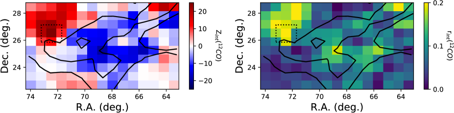
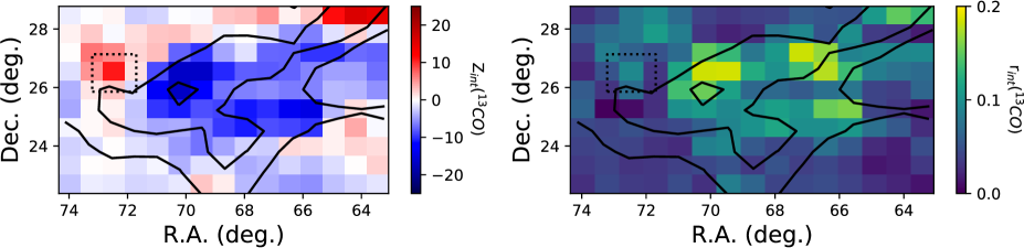
Figure 7: Images of the projected Rayleigh statistic, (left) $Z_{int}$ and (right) mean resultant vector, $r_{int}$ for ¹²CO (top) and ¹³CO (bottom) integrated over velocities 5 to 8 km s^-1  for each subfield. The dotted-line box in each panel shows the location and area of the demonstration field presented in Figure 2. The contours are identical to those in Figure 6.

5 Variation of relative orientations with gas properties

In the previous section, we find a broad range of relative orientations between thin-slice intensity gradients and the magnetic field. This diversity of orientations is not exclusively due to random errors but likely reflects spatial variations of conditions such as the magnetization, ion-neutral coupling, gas to magnetic flux ratios, efficiency of alignment of dust grains, or the projection of 3-dimensional quantities into the two-dimensional frame of the observations (Seifried et al., 2020). In this section, we examine the conditions in the cloud accessible from the ¹²CO, ¹³CO, and Planck data that may regulate the alignment of elongated turbulent eddies or gas flows with the magnetic field orientation.

5.1 Column Density

The neutral gas component of clouds is coupled to the interstellar magnetic field through collisions with ions. The ionization fraction of the gas is maintained by cosmic rays and the ultraviolet radiation field. In the low column density envelopes of molecular clouds, there is more exposure to ambient photoionizing radiation that can keep the neutral gas well coupled to the interstellar magnetic field. With a stronger coupling of ions and neutrals, it is reasonable to expect a stronger alignment of MHD turbulence or large scale flows with the magnetic field orientation in regions of low column density.

Figure 6 and Figure 7 show a stronger degree of alignment (large $Z_{k}$ and $Z_{int}$ values) of the vector normal to the thin-slice intensity gradient vector with the magnetic field in the outer edges of the ¹²CO and ¹³CO maps. This alignment is particularly strong in the northeast sector of the cloud in both ¹²CO and ¹³CO, where the magnetically aligned striations are found (Goldsmith et al., 2008; Heyer et al., 2016) and where PCA-derived velocity structure functions are anisotropic and aligned with the magnetic field orientation (Heyer et al., 2008; Heyer & Brunt, 2012). This region is characterized by low column densities inferred from visual extinction maps (Pineda et al., 2010) and Planck-derived opacity images (Planck Collaboration Int. XXXV, 2016) and low density, sub-thermal excitation conditions of ¹²CO and ¹³CO J=1-0 lines (Pineda et al., 2010). Conversely, in the central regions with higher column densities, there is a preferred perpendicular alignment.

Does this trend of relative orientations with column density hold throughout the cloud? To examine this question, we plot the variation of $Z_{int}$ values with column density over each subfield area in the upper left boxes of Figure 8 and Figure 9. The mean resultant vector for each subfield is encapsulated in the color of each point. To guide the eye, the vertical gray lines correspond to the drawn contour levels in Figure 6 and Figure 7. For both ¹²CO and ¹³CO  there are significant positive and negative values of $Z_{int}$ over the log(N(H)) range 21.5-21.75. Evidently, column density is not the only factor that determines whether turbulent eddies are aligned along the magnetic field.

At higher column densities, where one must be more cautious in interpreting the ¹²CO alignments owing to large line opacities, there is a clear excess of subfields with negative $Z_{int}$(¹²CO) values for log(N(H)) $>$ 21.75. This excess is also present when evaluated at higher resolutions (smaller subfield sizes) as shown in Figure 14. The degree of alignments in this high column density regime is best probed with lower opacity ¹³CO data (see Figure 9). Again, for log(N(H)) $>$ 21.75, there many more subfields with $Z_{int}$(¹³CO) values less than $-$3 corresponding to perpendicular alignment than those with values greater than 3 (see also Figure 15).

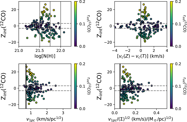
Figure 8: Variation of $Z_{int}$(¹²CO) values in each subfield with (top left) hydrogen column density derived from Planck and smoothed to subfield angular resolution with vertical gray lines marking the contour levels in Figure 6 and Figure 7, (top right) offset between first moments of $Z_{k}$ and $T_{k}$ with vertical line denoting zero offset, (bottom left) v_1pc, and (bottom right) v${}_{1pc}/\Sigma^{1/2}$. The color of each point represents the value of the mean resultant vector with yellow-green-teal points more reliable than blue-purple points. The horizontal dashed lines represent $|Z_{int}|/\sigma(Z_{int})=3$. The vertical solid lines in the bottom panels represent the mean values of v_1pc and v${}_{1pc}/\Sigma^{1/2}$ derived for Galactic clouds.

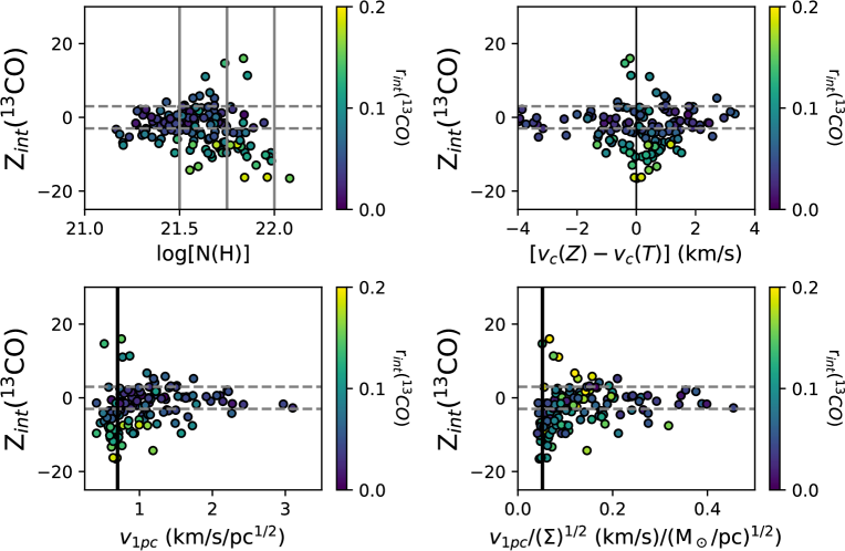
Figure 9: Same as Figure 8 for ¹³CO.

5.2 Velocity Displacement

In the demonstration field, we found that the peak value of the $Z_{k}$ spectrum is offset from the velocity centroid of the average ¹²CO and ¹³CO spectra over the subfield (see Figure 5). One possible reason for this displacement is reduced confusion along the line of sight as one is more kinematically displaced from the bulk of the emission or simply lower opacity in the line wings. To assess whether this displacement is a factor in aligning the thin-slice intensity gradient with the magnetic field orientation, we plot the variation of $Z_{k}$ with the difference of velocity centroids respectively calculated from $Z_{k}$ and the average brightness temperature spectrum, T(v), for each subfield. The results are shown in the upper right boxes of Figure 8 and Figure 9. For ¹²CO, this displacement is $\sim$ 0.5 km s^-1(redshifted) for both positive and negative values of $Z_{int}$. For ¹³CO  the distribution of velocity displacements of significant points ($r_{int}$ $>$ 0.1) is more centered on zero. This difference between ¹²CO and ¹³CO velocity displacements suggests that observed alignments are limited to lines of sight or velocity displacements where the line opacity is low. For ¹³CO, this condition is met at line center owing to its smaller abundance relative to ¹²CO. For ¹²CO, reduced optical depths over small velocity intervals, but still greater than unity, are possible in the wings of the spectral line profile. It is not clear why these displacements for ¹²CO are strongly skewed towards the redshifted side of the mean spectrum. We speculate that blue shifted material may be located on the backside of the cloud so any emission from this layer would cross multiple correlation lengths that may dilute any signature of alignment.

5.3 Normalizations of Turbulence

The alignment of turbulent eddies with the local magnetic field is a fundamental prediction of sub-Alfvénic MHD turbulence theories (Goldreich & Sridhar, 1995; Lazarian & Vishniac, 1999; Cho & Lazarian, 2003). Such alignment is also expected for magnetosonic waves (Mouschovias et al., 2011). Moreover, our analysis of thin-slice intensities of molecular line emission as a measure of the turbulent velocity field is based on Lazarian & Pogosyan (2000) who analytically demonstrated that intensity spatial variations in the thin-slice limit arise primarily from velocity fluctuations. A useful measure to characterize the degree of turbulence within an area is the velocity dispersion measured at 1 pc scale. This corresponds to the normalization coefficient of the first-order structure function but can be estimated by simply evaluating the velocity dispersion, $\sigma_{v}(L)$ over a scale, $L$ in pc, such that v${}_{1pc}=\sigma_{v}(L/2)/(L/2)^{1/2}$, which assumes the power law index of the structure function is 1/2. The cloud to cloud velocity dispersion-size relationship emerges from the near invariance of this value when integrated over the whole cloud (Larson, 1981; Heyer & Brunt, 2004). But this value can fluctuate within a cloud depending on local feedback processes from star formation or the dependency of this parameter with surface density (Heyer et al., 2009). A secondary measure of the turbulent motions is the quantity v_1pc/$\Sigma^{1/2}$, where $\Sigma$ is the mass surface density in units M_⊙/pc².

In the bottom rows of Figure 8 and Figure 9, we show the variation of $Z_{int}$ values with v${}_{1pc}=\sigma_{v}/(L/2)^{1/2}$ and v${}_{1pc}/\Sigma^{1/2}$ for each subfield. The velocity dispersions are derived from the second moments of the mean ¹²CO and ¹³CO spectra constructed from all spectra within a given subfield. Since all subfields have an identical size, 3.5 pc or $L/2$=1.75 pc, the dependency rests exclusively on the velocity dispersion. However, by casting the dependence as v_1pc, we can compare the values to those derived from more established cloud to cloud normalizations as shown by the vertical solid line. The mass surface densities for each subfield are taken from the smoothed and aligned Planck column density image.

The median values of v_1pc are 1.0 and 0.9 for ¹²CO and ¹³CO respectively with standard deviations of 0.4 and 0.7. The median values of v_1pc/$\Sigma^{1/2}$ are 0.12 and 0.10 for ¹²CO and ¹³CO respectively with standard deviations of 0.07 and 0.11. For both parameters, these median values are slightly larger than the values derived for Galactic clouds by Solomon et al. (1987); Heyer et al. (2009). There is no strong correlation of $Z_{int}$ with v_1pc or v${}_{1pc}/\Sigma^{1/2}$ in these plots. However, we note that the most extreme values of $Z_{int}(^{12}{\rm CO})$ and $Z_{int}(^{13}{\rm CO}$) have values of v_1pc and v${}_{1pc}/\Sigma^{1/2}$ close to that of Galactic clouds. Conversely, subfields with large values of these quantities have near zero $Z_{int}$ values corresponding to random orientations between the direction of intensity gradient normals and the magnetic field. The trend of strongly aligned gradients with Galactic values of v_1pc and v_1pc/$\Sigma^{1/2}$ suggests that alignments occur only in turbulent-quiet regions. Given the MHD simulation results that anisotropy is limited to regions with sub-Alfvénic motions, we speculate that such quiet regions also correspond to sub-Alfvénic conditions.

5.4 Line Opacity

The differential views of the Taurus cloud provided by ¹²CO and ¹³CO J=1-0 emission as shown in Figure 1 are a result of very different line opacities. The ¹²CO line is almost always optically thick in most conditions of molecular clouds where the ¹³CO line is optically thin for most lines of sight within a cloud. In this section we examine the relationships between gradient alignments, velocity displacement from the line center of the average spectrum of a subfield, ${\rm v}_{k}-{\rm v}_{c}$, and $R_{k}$, the ratio of ¹³CO to ¹²CO antenna temperatures in velocity slice $k$, for each subfield. $R_{k}$ provides an observational proxy to the ¹²CO optical depth of emission within a velocity channel.

$$R_{k}=\frac{\nu(^{13}{\rm CO})}{\nu(^{12}{\rm CO})}\;\frac{[J_{\nu}(T_{x}(^{13}{\rm CO}))-J_{\nu}(2.7)]}{[J_{\nu}(T_{x}(^{12}{\rm CO}))-J_{\nu}(2.7)]}\frac{[1-e^{-\tau_{k}(^{13}{\rm CO})}]}{[1-e^{-\tau_{k}(^{12}{\rm CO})}]}$$ (11)

where $\nu$ is the line rest frequency, $J_{\nu}(T)=1/(e^{h\nu/KT}-1)$, $T_{x}$ is the excitation temperature, and $\tau_{k}$ is the optical depth for channel $k$. By assuming $\tau_{k}(^{13}{\rm CO})=\tau_{k}(^{12}{\rm CO})/X_{iso}$, where $X_{iso}$ is the abundance ratio of ¹²CO to ¹³CO, and values for the excitation temperatures, one can estimate $\tau_{k}(^{12}{\rm CO})$ and $\tau_{k}(^{13}{\rm CO})$. $R_{k}$ increases with increasing optical depth for a given set of values of $X_{iso}$, $T_{x}(^{12}{\rm CO})$, and $T_{x}(^{13}{\rm CO})$.

To compile $R_{k}$ from the data, we constructed the mean ¹²CO and ¹³CO spectrum from all pixels in a subfield and aligned these spectra to the same spectral axis. Then, the observed ratio for that subfield is $R_{k}=\left<T_{k}(^{13}{\rm CO})\right>/\left<T_{k}(^{12}{\rm CO})\right>$. Random errors are propagated to derive $\sigma(R_{k})$. We consider the same set of velocity channels as those shown in Figure 6. Figure 10 shows the variation of observed $R_{k}$ values with velocity displacement with points colored by their $Z_{k}$ value. For clarity, we only show points with significant ($>3\sigma$) values of $R_{k}$ and $Z_{k}$. Curves of equation 11 are shown with opacity along the top axis for 2 values of $X_{iso}$ = 30 (dashed) and 60 (solid) and $T_{x}(^{13}{\rm CO})$=$T_{x}(^{12}{\rm CO})$=8 K (black) and $T_{x}(^{13}{\rm CO})$=6 K, $T_{x}(^{12}{\rm CO})$=8 K (gray) to show the effects of isotopic fractionation and subthermal excitation. Both plots show similar patterns. There is a broad distribution of points at low values of $R_{k}$ and a convergence of $R_{k}$ towards its peak at zero velocity displacement. Subfields with positive $Z_{k}$ values indicating gradient normals mostly aligned with the magnetic field orientation have low values of $R_{k}$ and optical depths that are low but still greater than 1. While the positive $Z_{k}$ subfields are distributed across the range of velocity displacements, there are more subfields with positive velocity displacements as noted in §5.2. Subfields with negative $Z_{k}$ values show a much broader distribution of $R_{k}$ values. In the right panel of Figure 10, the domain defined by $R_{k}>0.3$ is almost exclusively populated by subfields with $Z_{k}(^{13}{\rm CO})<0$.

The line opacity limits the depth to which our observations can probe over a given velocity interval. The high opacity of ¹²CO implies that one can detect gas layers at different velocities but not penetrate very deeply into a given layer. The surplus of positive $Z_{k}(^{12}{\rm CO})$ and $Z_{k}(^{13}{\rm CO})$ values with low $R_{k}$ suggests that reduced optical depths are necessary to measure surface brightness textures and recognize magnetically aligned features in molecular clouds. In contrast, subfields with thin slice intensity gradient normals mostly perpendicular to the magnetic field orientation (blue points) show a broader distribution of $R_{k}$ values corresponding to a larger range in line opacities for both ¹²CO and ¹³CO. The visibility of such features over a range of $R_{k}$ suggests that such orientations are less influenced by line opacity.

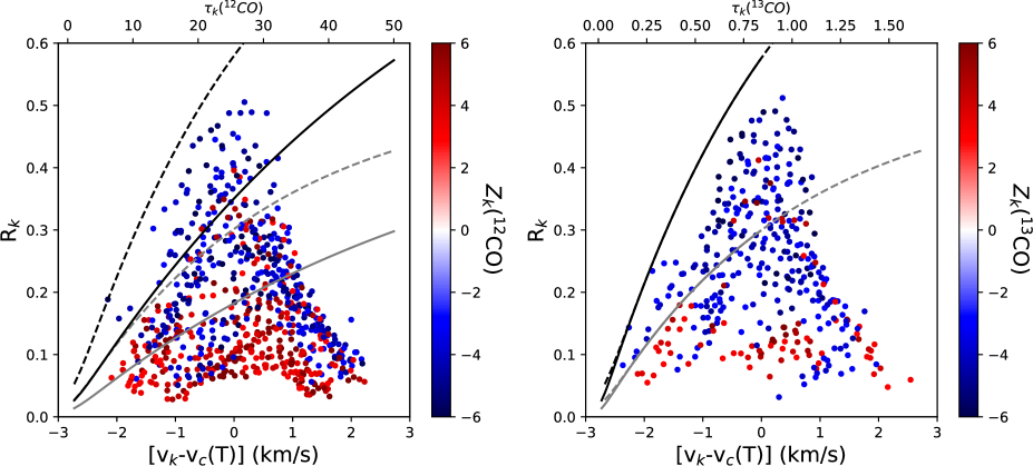
Figure 10: Plots of $R_{k}\equiv\left<T_{k}(^{13}{\rm CO})\right>/\left<T_{k}(^{12}{\rm CO})\right>$ values with velocity displacement for each subfield. Point colors represent $Z_{k}$ values indicating parallel (red) and perpendicular (blue) alignments for ¹²CO(left) and ¹³CO(right). Only subfields and velocity slices with $R_{k}/\sigma(R_{k})>3$ and $Z_{k}/\sigma(Z_{k})>3$ are shown. Curves show the variation of $R_{k}$ with optical depth (top axis) for $X_{iso}$=30 (dashed lines) and 60 (solid lines); $T_{x}(^{12}{\rm CO})$=8 K, $T_{x}(^{13}{\rm CO})$=8 K (black lines) and $T_{x}(^{12}{\rm CO})$=8 K, $T_{x}(^{13}{\rm CO})$=6 K (gray lines).

6 Discussion

Constraining the role of the interstellar magnetic field in molecular clouds is of paramount importance to our understanding of cloud evolution and star formation. A strong magnetic field with respect to a cloud’s self-gravity can slow the rate of collapse to account for the observed inefficiency of star formation (Mouschovias, 1987). Furthermore, the local Alfvénic Mach number, M_A, can influence the development of filaments, clumps, and cores and the topology of the magnetic field orientations.

Our images of $Z_{k}$ and $Z_{int}$ are roadmaps to the influence of the magnetic field upon the gas. We identify distinct regions in the Taurus cloud in which brightness temperature gradients are aligned parallel or perpendicular to the magnetic field orientations depending on location and line opacity (¹²CO or ¹³CO). We also find subfields where there is no preferred alignment.

The strong, parallel alignment of brightness temperature gradients with the magnetic field orientation, as in the northeast sector of the map, indicates that the motions are sub-Alfvénic (Lazarian & Yuen, 2018b). In this regime, the magnetic field configuration is not distorted by the isotropic turbulent motions. Rather, the gas motions are anisotropic and regulated by the magnetic field threading the cloud.

Our study confirms that the relative orientation becomes mostly perpendicular in subfields with hydrogen column densities in excess of 6$\times$10²¹ cm^-2. This is likely due to the effects of gravitational collapse in these dense regions (Chen et al., 2016; Soler & Hennebelle, 2017). If the dense filaments, which comprise much of the central region of the Taurus cloud, develop from material falling along a uniformly configured magnetic field due to gravity, then this naturally sets up perpendicular orientations of the ¹³CO brightess temperature gradients and the magnetic field orientation. Alternatively, large shocks driven by localized, supersonic yet sub-Alvénic flows channeled by the magnetic field would also generate filamentary structures perpendicular to the magnetic field (Chen & Ostriker, 2015; Mocz & Burkhart, 2018).

For both isotopologues, 33% to 50% of the subfields have $|Z_{int}|<$ 3 and no preferred orientation. In these areas, there is either 1) little signal, or 2) if any signal is present, the surface brightness in the thin slice channels is uniformly distributed, so there are no gradients or 3) the orientations of thin slice intensity gradients are randomly offset from the magnetic field orientations. Super-Alfvénic gas flows can be responsible for the last of these conditions as isotropic turbulence can scramble the orientations of the magnetic field. However at the 10′ resolution of the Planck measurements, the magnetic field orientations vary smoothly across most of the Taurus cloud indicative of sub-Alfvénic gas motions. So the absence of a preferred orientation is produced by the broad distribution of orientations of the intensity gradients with respect to a mostly uniform field and not to a distorted magnetic field. It is possible that the gas motions in these subfields are trans-Alfvénic, M_A $\sim 1$, such that the magnetic field configuration is not strongly distorted but the gas motions are less responsive to the local magnetization (Heyer & Brunt, 2012). This conjecture is supported by Hu et al. (2019) who derive an Alfvénic Mach number in Taurus of 1.1-1.2 by applying the Davis-Chandrasekhar-Fermi method to the distributions of Planck polarization angles and ¹³CO velocity centroid gradient angles.

Our analysis identifies subfields with intensity gradients parallel and perpendicular to the magnetic field orientation as well as subfields with no preferred alignment. These differential conditions suggests that the Alfvén Mach number varies within a cloud volume. Such inhomogeneity should be expected due to strong, localized, density fluctuations in a supersonic medium and the $\rho^{-1/2}$ dependency, where $\rho$ is the mass volume density. Given the density inhomogeneity of molecular clouds, there are necessarily pockets of large and small Alfvénic Mach numbers (Burkhart et al., 2009). This is an important observational insight, as it suggests to simulators and theorists that there may not be one magnetic state within a cloud domain. Consequently, there should be a range of possible star formation scenarios within the domain of a single cloud.

7 Conclusions

We have examined the relative orientations between the interstellar magnetic field and spatial derivatives of antenna temperatures within thin velocity slice images of ¹²CO and ¹³CO J=1-0 emission from the Taurus molecular cloud. Our analysis includes a robust treatment of random errors in the relative orientations produced by the thermal noise of the spectroscopic and polarization data. The relative orientations within subfields of the cloud are parameterized by the projected Rayleigh statistic and the mean resultant vector that are derived for both thin-sliced velocity channels and integrated over a broader velocity interval. Images of the projected Rayleigh statistic show mostly parallel alignments of the vector normal to the intensity gradient and the component of the interstellar magnetic field in the plane of the sky for subfields in the outer periphery of the cloud and in subfields with reduced ¹²CO optical depths. This relative orientation becomes mostly perpendicular in subfields in the central regions of the cloud with hydrogen column densities greater than 6$\times$10²¹ cm^-2. The strongest alignments (parallel or perpendicular) occur in regions for which measures of the amplitude of turbulent motions are comparable to values found in Galactic clouds. There are other sections of the cloud where there is no preferred alignment of gradients with the magnetic field that may imply a transition to trans-Alfvénic Mach numbers but could also be a result of projection effects along the line of sight or inefficient grain alignment with the local magnetic field. This diversity of alignments imply changing levels of magnetization within the cloud volume. Such inhomogeneity should be considered when addressing the evolution of molecular clouds and the formation of stars.

Data Availability

The data underlying this article will be shared on reasonable request to the corresponding author.

Appendix A Instrumental Errors

The analysis of spatial gradients of two-dimensional fields is a powerful tool that quantifies the rich structure and texture of molecular line emission or thermal dust emission. However, the derived gradients of observational data are sensitive to the random errors of the measurements. For line emission, uncertainties of observed brightness temperatures arise from fluctuations of the radiometer and those of the atmosphere through which the measurements are collected. The root mean square (rms) fluctuations due to thermal noise can be derived for each spectrum by simply calculating the standard deviation of values in spectral channels with no emission. These errors propagate through the calculation of the gradient magnitude and direction (equations 1 and 2). To assess the impact of instrumental errors on the gradient vector, we use the Monte Carlo method for its simplicity.

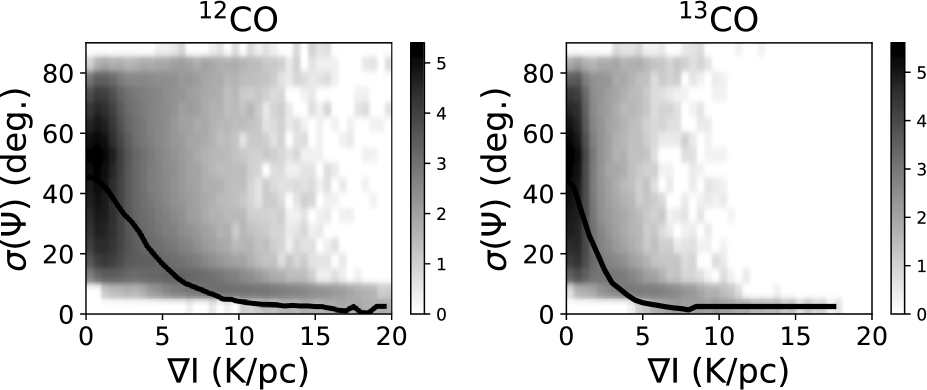
Figure 11: A two-dimensional histogram of random errors of the gradient angle, $\sigma(\Psi)$ and the magnitude of the intensity gradient, $\nabla$I, for ¹²CO(left) and ¹³CO (right). The shading of the histogram is log(N), where N is the number of points in each two-dimensional bin. The solid line shows the median value of $\sigma(\Psi)$ for each bin of $\nabla$I. The gradient angle, $\Psi$ is only well defined ($\sigma(\Psi)<15^{\circ}$) for gradients larger than 4 K/pc (¹²CO) and 2.2 K/pc (¹³CO).

We summarize the Monte Carlo derived errors in $\Psi_{G,k}$ in Figure 11, which shows a two dimensional histogram in bins of $\sigma(\Psi_{G,k})$ and the gradient magnitude, $\nabla T_{k}$ for both ¹²CO and ¹³CO. Each histogram is constructed from almost 16 million values corresponding to 1024 samples for each subfield, 150 subfields, and 104 spectral channels. For each $\nabla T_{k}$ bin, we derive the median value of $\sigma(\Psi_{G,k})$, which is shown as the solid, dark line in Figure 11. The median values decrease with increasing gradient magnitude. For small gradient magnitudes, the errors in the gradient direction are quite large as expected for a random distribution. For display purposes only (see Figures 2,3), we determine the value of the gradient magnitude at which $\sigma(\Psi_{G,k})$ is less than 15^∘ for each CO isotopologue. These threshold values are 4 K/pc and 2.2 K/pc for ¹²CO and ¹³CO respectively.

Instrumental uncertainties also affect the polarization angle, $\Psi_{E}$ from which we infer the orientation of the interstellar magnetic field assuming the alignment of elongated grains. The error in the polarization angle is derived from the errors in the $U$ and $Q$ Stokes parameters. We do not add any error terms in the rotation of the polarization angle by 90^∘ to derive $\Psi_{B}$. The distribution of errors in $\Psi_{B}$ are shown in Figure 12. The mean error is 7.3^∘ with a standard deviation of 1.6^∘.

The resultant errors in the gradient direction as well as errors in the dust polarization orientation that arise from uncertainties in the $U$ and $Q$ Stokes parameters are added in quadrature to determine the error in the relative orientation, $\sigma(\Phi)$ for each sampled position. The errors in the gradient calculation make the largest contribution to the uncertainties of the relative orientation, $\Phi_{k}$, for all but the largest gradients. This composite error value is used when weighting the sums for the Rayleigh statistic and the mean resultant vector. For the thin-slice channels with no emission, the $Z_{k}$ values are all near zero as expected for a random distribution of angles derived from noise as shown for a single subfield in Figure 5. Moreover, the random errors in $Z_{k}$ derived from propagating the Monte-Carlo produced distributions of $\Psi_{G,k}$, are comparable to the predicted values (Jow et al., 2018).

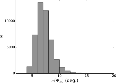
Figure 12: A histogram of the instrumental errors of the magnetic field orientation, $\sigma(\Psi_{B})$ as derived from the uncertainties of the Planck 353 GHz $U$ and $Q$ Stokes parameters. The median error is 7^∘. Random errors of the relative orientation, $\sigma(\Phi)$ are dominated by those of the gradient.

Appendix B Correlation between $r_{int}$ and $Z_{int}$

In §4.2, we use the mean resultant vector, $r_{int}$ as a guide to interpret the signficance of $Z_{int}$ values. In Figure 13, we show the variation of $Z_{int}$ values with $r_{int}$ for all 150 subfields to evaluate the connection between the two statistics and to define a threshold value of $r_{int}$ above which one can have confidence in the $Z_{int}$ value. The dashed horizontal lines denote $|Z_{int}|/\sigma(Z_{int})=3$ Within the 3$\sigma$ limits, there is a cluster of points with $r_{int}<0.05$ that arises from subfields with little or no signal. For $r_{int}>0.1$, the two statistics correlate very well. Examining Figure 7, one should place more confidence in $Z_{int}$ values with $r_{int}$ values above this threshold.

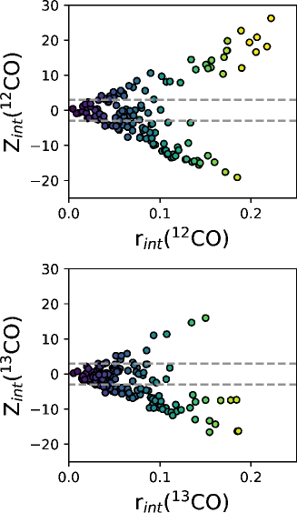
Figure 13: Variation of the Rayleigh statistic, $Z_{int}$, with the mean resultant vector, $r_{int}$ for ¹²CO(top) and ¹³CO(bottom). The dashed horizontal lines denote 3$\sigma(Z_{int})$ values. The color coding of points is the same as in Figure 7 and Figure 8. $Z_{int}$ correlates well with $r_{int}$ for $r_{int}>0.1$.

Appendix C Resolution Study

For our study, the angular resolution of the Rayleigh statistic is set by the size of the subfields. In Figure 6 and Figure 7, each subfield is comprised of 256$\times$256 pixels and subfields are spaced from each other by 128 pixels. When calculating the Rayleigh statistic (equations 4 and 8) and the mean resultant vector (equations 9-11), the subfield is sampled at 8 pixel intervals, which provides 1024 relative orientation angles for each subfield. However, as Figure 2 demonstrates, there are temperature brightness variations in the ¹²CO and ¹³CO thin-slice images. Small scale variations of $\Phi$ values could impact the value of the Rayleigh statistic when summed over a given area.

To assess the effects of resolution on the value of $Z_{int}$, we have constructed images of the Rayleigh statistic within subfields sizes of 128$\times$128 pixels and 64$\times$64 pixels. The subfields are spaced by 128 and 64 pixels respectively. These resolutions provide 256 and 64 samples for each subfield. The results are shown in Figure 14 for both ¹²CO and ¹³CO. In general, the $Z_{int}$ images at these higher resolutions are similar to those shown in Figure 7 but with lower values of $Z_{int}$. Since $Z_{int}$ is an additive, unnormalized quantity, the absolute value of $Z_{int}$ decreases with decreasing number of $\Phi_{k}$ values.

Since the Taurus cloud exhibits strong spatial variations in hydrogen column density, the lower resolution information on $Z_{int}$ and N_H could smooth over small scale correlations between these 2 quantities. Figure 15 shows the variation of $Z_{int}$ values with hydrogen column density for these higher resolutions. Similar trends that are identified in Figure 8 and Figure 9 are also evident at these higher resolutions but extend to higher column density values owing to the finer resolution. No new trends emerge from the higher resolution images.

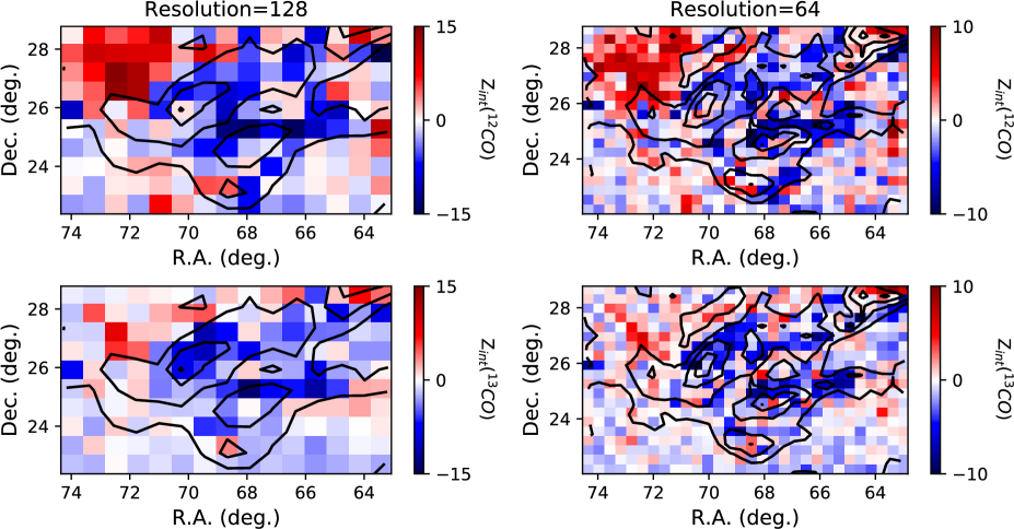
Figure 14: Images of the Rayleigh statistic, $Z_{int}$, for resolutions of 128 pixels (left) and 64 pixels (right) for both ¹²CO (top) and ¹³CO (bottom). Black contours show the distribution of hydrogen column density at these same resolutions.

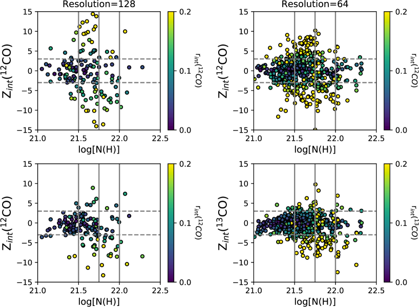
Figure 15: Variation of $Z_{int}$(¹²CO) (top) and $Z_{int}$(¹³CO) (bottom) with hydrogen column density in each subfield with resolutions of 128 pixels (left) and 64 pixels (right). The color coding of points reflect $r_{int}$ values calculated with these same resolutions.

References

- Arons & Max (1975) Arons J., Max C. E., 1975, ApJ, 196, L77
- Astropy Collaboration et al. (2013) Astropy Collaboration et al., 2013, A&A, 558, A33
- Brunt & Mac Low (2004) Brunt C. M., Mac Low M.-M., 2004, ApJ, 604, 196
- Burkhart et al. (2009) Burkhart B., Falceta-Gonçalves D., Kowal G., Lazarian A., 2009, ApJ, 693, 250
- Burkhart et al. (2014) Burkhart B., Lazarian A., Leão I. C., de Medeiros J. R., Esquivel A., 2014, ApJ, 790, 130
- Cabral & Leedom (1993) Cabral B., Leedom L. C., 1993, in Special Interest Group on GRAPHics and Interactive Techniques Proceedings.. Special Interest Group on GRAPHics and Interactive Techniques Proceedings.. pp 263––270
- Chandrasekhar & Fermi (1953) Chandrasekhar S., Fermi E., 1953, ApJ, 118, 113
- Chen & Ostriker (2015) Chen C.-Y., Ostriker E. C., 2015, ApJ, 810, 126
- Chen et al. (2016) Chen C.-Y., King P. K., Li Z.-Y., 2016, ApJ, 829, 84
- Cho & Lazarian (2003) Cho J., Lazarian A., 2003, MNRAS, 345, 325
- Clark et al. (2019) Clark S. E., Peek J. E. G., Miville-Deschênes M. A., 2019, ApJ, 874, 171
- Davis & Greenstein (1951) Davis Leverett J., Greenstein J. L., 1951, ApJ, 114, 206