Tracking the Footprints of Spin Fluctuations:
A MultiMethod, MultiMessenger Study of the Two-Dimensional Hubbard Model
Abstract
The Hubbard model represents the fundamental model for interacting quantum systems and electronic correlations. Using the two-dimensional half-filled Hubbard model at weak coupling as testing grounds, we perform a comparative study of a comprehensive set of state of the art quantum many-body methods. Upon cooling into its insulating antiferromagnetic ground-state, the model hosts a rich sequence of distinct physical regimes with crossovers between a high-temperature incoherent regime, an intermediate temperature metallic regime and a low-temperature insulating regime with a pseudogap created by antiferromagnetic fluctuations. We assess the ability of each method to properly address these physical regimes and crossovers through the computation of several observables probing both quasiparticle properties and magnetic correlations, with two numerically exact methods (diagrammatic and determinantal quantum Monte Carlo) serving as a benchmark. By combining computational results and analytical insights, we elucidate the nature and role of spin fluctuations in each of these regimes. Based on this analysis, we explain how quasiparticles can coexist with increasingly long-range antiferromagnetic correlations, and why dynamical mean-field theory is found to provide a remarkably accurate approximation of local quantities in the metallic regime. We also critically discuss whether imaginary time methods are able to capture the non-Fermi liquid singularities of this fully nested system.
pacs:
71.27.+a, 71.10.Fd, 73.43.NqI Introduction
I.1 Purpose of this article
The Hubbard model Hubbard (1963, 1964); Gutzwiller (1963); Kanamori (1963) has, for interacting quantum systems, a similar status as the Ising model for classical phase transitions and magnetism. It is the simplest possible model that can be considered, which nonetheless captures essential aspects of the physical phenomena of interest. In relation to materials with strong electronic correlations, the Hubbard model in its simplest form (especially, with a single band) is at best an approximation to reality. However, experimental progress in the field of cold atomic gases in optical lattices now yield rather accurate physical realizations of this simple model in the laboratory Jaksch and Zoller (2005); Bloch (2005); Lewenstein et al. (2007).
In contrast to the Ising model however, our current understanding of the Hubbard model is still lacunary. A thorough understanding can be reached in the limiting cases of one dimension Essler et al. (2005) and infinite dimensions (infinite lattice connectivity) Metzner and Vollhardt (1989); Georges and Kotliar (1992); Jarrell (1992), thanks to efficient analytical and computational methods available in these limits. In contrast, the two-dimensional case relevant to both cuprate superconductors Keimer et al. (2015); Timusk and Statt (1999); Norman et al. (2005); Lee et al. (2006) and cold atomic gases Jaksch and Zoller (2005); Bloch (2005); Lewenstein et al. (2007) still holds many open questions, both in relation to its phase diagram as a function of interaction, particle density and temperature, and regarding the nature of excited states as well as response functions and transport properties. There is a broad consensus in the community that progress on these outstanding issues is essential, even if addressed through the deceptively simple-looking Hubbard model.
In recent years, a number of computational methods have been developed to this end. In this context, it is of crucial importance to interrogate these methods regarding their respective ability to address regimes of physical interest. Furthermore, increasing emphasis is being put on establishing definite results with controlled computational methods, which can then serve as benchmarks LeBlanc et al. (2015); Motta et al. (2017); Williams et al. (2020) for approximate, often more flexible and computationally efficient methods.
Here we focus on a regime of the Hubbard model which is simple at first sight but, as we shall see, deceptively so: small interaction values (often referred to as “weak coupling”) and half-filling on the square lattice with nearest-neighbour hopping. The main purpose of this article is to assess the ability of state-of-the-art computational methods to address the finite-temperature physics of the model in this regime. We provide an extensive comparison between basically all methods currently available for this purpose, with two distinct Monte Carlo methods serving as reference benchmarks. Despite the apparent simplicity of this regime, we shall see that all methods face rather severe limitations, especially regarding the lowest temperature that can currently be reached. Our study also interrogates the model through a set of different physical observables, spanning thermodynamic properties, single-particle correlation functions (the Green function and associated self-energy) as well as two-particle correlations (the spin correlation function and correlation length). Because of this wide spectrum of both methods and observables, we have borrowed terminology from the astrophysics community in designating our work as a ‘multi-method, multi messenger study’ Neronov (2019).
Despite the deceptive simplicity of the two-dimensional Hubbard model in this parameter regime, the physics is quite rich and non-trivial. As is well established, the ground-state is an antiferromagnetic insulator which can be qualitatively understood using Slater’s classic description Slater (1951). However, finite-temperature properties display a rich sequence of interesting crossovers between physically distinct regimes as the system is cooled down towards its antiferromagnetic insulating ground-state. Two key features make these finite-temperature properties and crossovers non-trivial: (i) the fact that, despite perfect nesting, fluctuations destroy antiferromagnetic long-range order at any non-zero temperature - while the correlation length being exponentially large (Mermin-Wagner theorem Mermin and Wagner (1966); Hohenberg (1967)) and (ii) the van Hove singularity present at the ‘antinodal’ points of the Fermi surface, which further suppresses coherence of single-particle excitations near these points. Furthermore, the perfect nesting of the Fermi surface in combination with two-dimensionality leads to a departure from Fermi-liquid behavior in the metallic regime.
Another important goal of this article is therefore to discuss and characterize these different physical regimes and crossovers in details, with a particular focus on assessing the ability of the different methods to capture their physics properly. By combining computational results and analytical insights, we elucidate in particular the role and nature of spin fluctuations in the different regimes. As we shall see, this reveals some unexpected features of the metallic regime which are likely to have broader implications for materials with electronic correlations. Furthermore, we discuss whether the imaginary time computational methods considered in this article are able to probe the subtle non-Fermi liquid singularities of the metallic state caused by the perfect nesting of the Fermi surface. This rich physics thus makes this regime of the Hubbard model a perfect opportunity for systematic benchmarks, as well as useful testing grounds for future work on more complex regimes of parameters as well as real materials.
I.2 Overview of the methods assessed
We categorize the algorithms considered in this article into the following groups:
-
•
Benchmark methods. We consider two very different Monte Carlo methods. The first one is determinantal quantum Monte Carlo (DQMC, Blankenbecler et al. (1981)), the other one is the diagrammatic Monte Carlo method (further referred to as DiagMC) Prokof’ev and Svistunov (1998) (in its recent connected determinant implementation [CDet] for connected one-particle reducible quantities Rossi (2017) and DDMC for one-particle irreducible quantities Šimkovic and Kozik (2019); Moutenet et al. (2018), respectively). The reason for their application is twofold: (i) The methods are controlled and, hence, in the regime where they can be applied and converged, these methods are numerically exact. Therefore they are serving as a benchmark for the other approximate methods considered in this article. (ii) The regimes where the methods actually break down will be assessed - a crucial information in relation to their application to more challenging regimes. For both benchmark methods, we show error bars in the figures (which may, however, be smaller than the respective symbol sizes). All data points in this manuscript obtained by these methods are numerically exact.
-
•
Mean field methods. In Sec. III, we discuss dynamical mean-field theory (DMFT, Georges et al. (1996)) as a reference point beyond which spatial fluctuations must be included to properly address the two-dimensional model. In that section, we also briefly discuss simple static mean-field theory (MFT). As we shall see, DMFT provides a good starting point for our study and, remarkably, yields an accurate approximation of local observables through most of the metallic regime.
-
•
Cluster extensions of DMFT. The dynamical cluster approximation (DCA), and cellular DMFT (CDMFT) provide one possible route to systematically include spatial correlations within the DMFT framework, beyond the single-site approximation Maier et al. (2005a); Kotliar et al. (2006); Tremblay et al. (2006); Lichtenstein and Katsnelson (2000). Note that cluster-based methods (like CDMFT, DCA and also cluster-TRILEX, see next paragraph) are controlled methods with the control parameter being the size of the cluster. However, in some regimes shown in this paper (low temperatures) these algorithms could not be converged as a function of cluster size (for reasons explained in App. D.5 and D.6).
-
•
Vertex based extensions of DMFT. Another route for including spatial correlations beyond single-site DMFT is relying on higher order Green functions (vertex functions). In the main text we present results from the dynamical vertex approximation (DA, ladder version), the triply irreducible local expansion (TRILEX) in various flavors, the dual fermion (DF, ladder version) and the dual boson (DB, single-shot) approach Rohringer et al. (2018a).
-
•
Other approaches: in this category we show results from the two-particle self-consistent approach (TPSC, TPSC+, Vilk and Tremblay (1997); Tremblay (2011); Wang et al. ), the functional renormalization group (fRG Metzner et al. (2012), here considered up to one loop with Katanin substitution) and the parquet approximation (PA De Dominicis and Martin (1964a); Bickers (2004)).
This list covers the vast majority of currently available computational methods able to address finite temperature properties. One notable exception is the minimally entangled typical thermal state method (METTS) and related approaches, which combine together tensor network representations and stochastic sampling White (2009); Stoudenmire and White (2010); Bruognolo et al. (2015); Wietek et al. (2020). A systematic exploration of this method as applied to the Hubbard model is currently being actively pursued by several groups and comparisons with the present methods will have to be performed in future work Wietek et al. (2021).
The basic principles of each of these methods, useful references for further reading and results from slightly differing implementations of the respective methods and algorithms are summarized in App. D. Throughout the paper we consider the interaction value of . Let us stress from the outset that, despite this rather moderate interaction value, each of these methods encounters limitations in their regime of applicability. These limitations stem either from (i) the approximation performed or (ii) algorithmic obstacles.
We find that the lowest reachable temperature for the DiagMC algorithm is . In this case, reaching lower temperatures is hindered by the difficulty in summing the perturbative series. Interestingly, we find that the limitation of the DQMC algorithm is similar, . In that case, the limitations originate from the exponentially growing correlation length which would require the simulation of prohibitively large systems at lower . DMFT, in contrast, can be converged to very low temperatures and also at . Self-consistent methods (e.g. TRILEX) suffer from convergence problems at low-, whereas calculations involving a ‘single-shot’ correction beyond DMFT without self-consistency such as DA, DB or DF can be performed as long as the correlation length can be accurately resolved (DA, DB) or, for DF, as long as the starting point - paramagnetically restricted DMFT - remains reasonably accurate. The finite momentum grid also limits the application of fRG and PA, and, to a lesser degree, TPSC and TPSC+. An intrinsic limitation of TPSC occurs in the renormalized classical regime (see App. D.11) leading to a rather severe overestimate of the onset temperature of the pseudogap. TPSC+ has been proposed to remedy this: in the present paper, the first application of TPSC+ is actually presented, but its applicability has yet to be explored more widely. An obvious limitation of quantum cluster theories are the cluster sizes which they can reach, which have to be compared to the correlation length - a very demanding criterion in the present case, as will be shown later.
I.3 Definition of the model, the role of the van Hove singularity and nesting
We consider the single-band Hubbard model defined by the following Hamiltonian:
| (1) |
where is the (nearest-neighbor) hopping amplitude, denotes summation over nearest-neighbor lattice sites, the electron’s spin, the strength of the (purely local) Coulomb interaction and the spin resolved number operator. Throughout the paper all energies are given in units of . Furthermore we set and . We consider the case of (usually regarded as “weak coupling”) at half-filling , corresponding to a chemical potential of and the simple square lattice, resulting in the following dispersion relation for the electrons (lattice constant ):
| (2) |
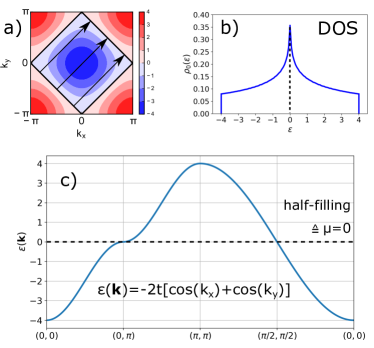
The particular form of the dispersion and the case of half-filling leads to a very peculiar diamond-shaped Fermi surface, already resulting in an interesting behavior without interactions present: (i) it exhibits a (“perfect”) nesting by the momentum vector , which connects every Fermi surface point to another respective one (see Fig. 1), leading to an enhanced susceptibility at and (ii) the momenta around the (stationary) antinodal Fermi surface point imply a logarithmic divergence in the density of states at the Fermi level (van Hove singularity, Fig. 1), leading to a larger scattering phase space than at the nodal point . Furthermore, because we consider only nearest-neighbor hopping, the diamond-shaped Fermi surface displays perfect nesting by the whole family of wave vectors of the form , with consequences for the nature of the metallic regime.
I.4 Organization of this article
This article is organized as follows: In Sec. II, we describe the different physical regimes encountered in this model as a function of temperature, using results from our two benchmarks methods (DiagMC and DQMC). In Sec. III, we discuss dynamical mean-field theory, which serves as a starting point of several approximate methods considered in this article. In Sec. IV, we discuss the calculation of single-particle properties using all the different methods introduced above. In Sec. V, we discuss the -dependence of the double occupancy and its physical significance. In Sec. VI, we discuss two-particle response functions and the -dependence of the magnetic correlation length. In Sec. VII, we discuss the implications of our computational results for the physics of spin fluctuations in this model. Finally, a discussion and conclusions are provided in Sec. VIII. A number of appendices present more technical points as well as details of the different methods. As Supplemental Material Sup we provide all the numerical data used in the figures of the main text.
| method | ||||||
|---|---|---|---|---|---|---|
| DiagMC | 0.42 | 0.35 | 0.065 | 0.0625 | 0 | |
| DQMC | 0.42 | 0.35 | 0.065 | 0.0625 | 0 | |
| MFT | 0.2 | 0.2 | 0.2 | |||
| DMFT | 0.45 | 0.45 | 0.08 | 0.08 | 0.08 | |
| DCA, N=128 (PM enforced) | 0.42 | 0.35 | ? | ? | - | |
| CDMFT, N=64 (PM enforced) | 0.45 | 0.42 | ? | ? | see Sec. VI | |
| CDMFT+CFE, N=64 (PM enforced) | 0.42 | 0.35 | ? | ? | see Sec. VI | |
| DA (ladder) | 0.42 | 0.35 | 0.065 | 0.059 | 0 Katanin et al. (2009); Rohringer and Toschi (2016, 2020) | |
| DF (ladder) | 0.44 | 0.37 | 0.062 | 0.06 | 0 (?) | |
| DB (single-shot) | 0.42 | 0.35 | 0.07 | 0.07 | 0 (?) | |
| TRILEX | 0.44 | 0.35 | 0.055 | 0.055 | 0 (?) | |
| TRILEX, | 0.44 | 0.35 | 0.055 | 0.055 | 0 (?) | |
| TRILEX, N=2 | 0.44 | 0.35 | 0.055 | 0.055 | 0 (?) | |
| TRILEX, N=4 | 0.44 | 0.35 | 0.055 | 0.055 | 0 (?) | |
| TPSC | 0.42 | 0.29 | 0.13 | 0.1 | 0 | |
| TPSC+ | 0.44 | 0.37 | 0.07 | 0.07 | 0 | |
| fRG (one-loop Katanin) | 0.42 | 0.35 | 0.08 | - Baier et al. (2004); Kugler and von Delft (2018a, b); Hille et al. (2020a, b) | 0 Bickers and Scalapino (1992); Baier et al. (2004); Eckhardt et al. (2018, 2020) | |
| PA | 0.44 | 0.37 | 0.05 | 0.05 | 0 Bickers and Scalapino (1992); Eckhardt et al. (2018, 2020) |
II Qualitative description: physical regimes and crossovers
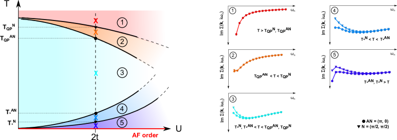
Before presenting detailed results from a variety of many-body approaches in Sec. III-VI, in this Section we sketch the overall physical picture which emerges from this study in Fig. 2 (see also Schäfer et al. (2015a); Šimkovic et al. (2020); Kim et al. (2020)). The left panel indicates in a schematic manner the key crossover scales that delimit different physical regions as a function of temperature , for a given value of . Our quantitative study focuses on but the qualitative statements made here are expected to apply throughout the weak to intermediate coupling regime (see e.g. Tanaka (2019) for a study of the evolution to higher couplings). As the system is cooled down from high temperature, we observe several regimes with qualitatively different physical properties (a quantitative criterion for the onset of these scales will be given at the end of the section).
At high temperature, thermal fluctuations prevent the formation of long-lived quasiparticles: this regime can be thought as an ‘incoherent soup’ of fermions above their degeneracy temperature and is depicted as the red shaded area ① in Fig. 2. Cooling the system progressively extinguishes these thermal fluctuations, leading to increased coherence in the single-particle spectrum and the appearance of long-lived quasiparticles. Here and below, we use the term ‘quasiparticle’ in a general and somewhat loose sense of a dispersing single-particle excitation with a ‘long enough’ lifetime. For the specific model at hand, because of perfect nesting, the ‘quasiparticles’ do not obey Landau Fermi liquid theory however: this is discussed in more details in Sec. VII.3.3. At the node, this quasiparticle coherence scale corresponds to the temperature at which the thermal de Broglie wavelength along the nodal direction becomes larger than the lattice spacing, with being the effective Fermi velocity renormalized by interactions. The metallic regime is depicted as region ③ (light blue) in Fig. 2.
The crossover scale associated with the passage from region ① to region ③ is not the same all along the Fermi surface however. Because of the van Hove singularity stemming from the antinodal points of the Fermi surface such as (see Sec. I.3), the coherence temperature at the nodal point is higher than the coherence temperature at the antinodal point . This defines an extended crossover region ② in which the system is coherent near the nodes but still incoherent near the antinodes (orange shaded area in Fig. 2).
Although further lowering the temperature in the metallic regime ③ initially results in freezing out thermal fluctuations and hence in an increase of the quasiparticle lifetime, this does not persist down to the lowest temperature. Indeed, antiferromagnetic correlations develop as is lowered, with an exponentially growing correlation length, eventually diverging at when the ground-state with antiferromagnetic long-range order is reached.
In this low- regime, long-wavelength antiferromagnetic fluctuations (Slater paramagnons) lead to an enhancement of the quasiparticle scattering rate upon cooling and to the formation of a pseudogap in the single-particle spectrum, which evolves into a sharp gap in the Slater-like insulator at Slater (1951). Once again, the crossover temperature corresponding to the suppression of coherence and the opening of the pseudogap is not uniform along the Fermi surface: it is larger at the antinodes where the destruction of coherence occurs first upon cooling, and smaller at the nodes: . Hence, in the dark blue shaded area ④ where , one has a partially (pseudo-)gapped Fermi surface. Eventually, all states of the Fermi surface are suppressed by antiferromagnetic fluctuations for resulting in a fully open pseudogap everywhere on the Fermi surface (purple shaded area ⑤). Let us stress again that long-range antiferromagnetic order and a true gap only sets in at as a consequence of the Mermin-Wagner theorem Mermin and Wagner (1966); Hohenberg (1967).
Since all the temperature scales described above correspond to crossovers, an appropriate criterion must be defined to identify and quantify them. These scales mostly refer to the presence or absence of characteristic spectral features in the single-particle properties, and hence an obvious observable would be the momentum- and energy- resolved spectral function: and corresponding self-energy as a function of real frequency (see also App. B and Rohringer and Toschi (2016)). However, as all the methods considered in the following are formulated on the Matsubara (imaginary) frequency axis, a much more practical criterion can be obtained via the imaginary frequency dependence of the (imaginary part of the) momentum-resolved self-energy , consistently with previous work Schäfer et al. (2015a, 2016a); Šimkovic et al. (2020). Representative results for this quantity in the five different regimes discussed above are displayed on the right panel of Fig. 2. At high temperature, the thermal fluctuations lead to a divergent behavior of at low frequencies. can thus be defined as the temperature where this divergent behavior is eased, i.e. when the slope between the first and second Matsubara frequency changes sign and becomes negative Schäfer et al. (2015a, 2016a); Šimkovic et al. (2020). In the metallic regime (region ③), the behavior of over the lowest Matsubara frequencies can be approximated by a Taylor series . In a standard Fermi liquid, and are the quasiparticle spectral weight () and inverse quasiparticle lifetime, respectively (see App. B for details and a critical discussion). Likewise, the onset of insulating/pseudogapped behaviour at is signalled by an additional change of slope, which becomes positive again at lower temperatures. The actual quantitative criterion for extracting the data of Tab. 1 using the quasiparticle weight is also discussed in App. B.
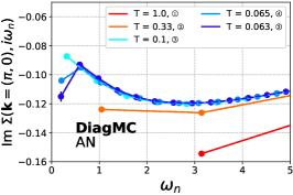
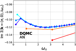
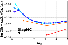
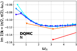
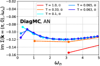
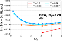
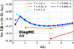
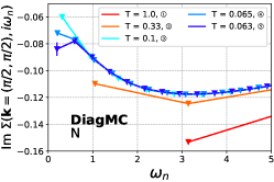
To illustrate the onset of these different regimes at the one particle level, we display in Fig. 3 results for the imaginary part of the self-energy on the Matsubara axis calculated with the two numerically exact methods used in this paper, namely diagrammatic Monte Carlo (DiagMC, left panels, see App. D.1) and determinantal quantum Monte Carlo (DQMC, right panels, for technical details, including finite size scaling and Trotter extrapolation see App. D.2, for preceding works see also Rost et al. (2012); Schäfer et al. (2015a); Rost and Blümer (2015)). Both exact methods shown in Fig. 3 exhibit and with a momentum differentiation between antinode (upper panels) and node (lower panels) with and for the onset of the quasiparticle coherence and and for the onset of the insulating behavior (more intermediate temperatures have been calculated for the extraction, see Fig. 19 and App. B). DiagMC and DQMC are in agreement within error bars and (for the one-particle quantities) are able to be converged until . With the aim of giving an overview and for further reference, we summarize in Table 1 the results of each of the different methods investigated below for the crossover temperatures delimiting the five distinct regimes discussed above.
III The dynamical mean-field reference point and the role of fluctuations
Several methods considered in the following use dynamical mean-field theory (DMFT) as a starting point. Within DMFT, local fluctuations are taken into account (i.e. quantum and thermal fluctuations between the four possible local states on each site), but spatial fluctuations are not. In the two-dimensional model considered here, these fluctuations are strong and DMFT should be viewed as a zeroth-order approximation, which needs to be extended in order to take these fluctuations into account. DMFT is exact in the formal limit of infinite dimensions or infinite lattice connectivity, in which spatial fluctuations do become negligible Metzner and Vollhardt (1989); Georges and Kotliar (1992).
III.1 Self-energies and quasiparticle coherence
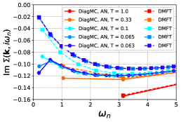
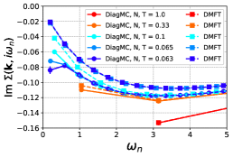
Because non-local fluctuations are neglected, the self-energy is approximated within DMFT by a function which is local in real space, i.e. independent of momentum. In Fig. 4, we display the DMFT self-energy for several temperatures, and compare it to the benchmark (DiagMC) result for both the antinodal and nodal points (left and central panel, respectively). It is seen that the DMFT approximation is accurate at very high temperatures, where indeed correlations are very local (as shown below, the magnetic correlation length is only a couple of lattice spacing down to ). Deviations between the DMFT self-energy and the DiagMC benchmark are already apparent at : at this temperature, these deviations are small at the nodal point but already significant at the antinodal point due to the proximity of the van Hove singularity and the resulting momentum-dependence of the self-energy.
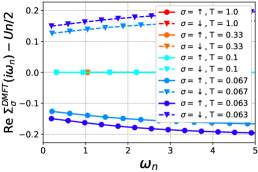
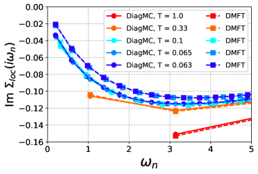
It is interesting to note, however, that the local component of the self-energy (i.e on-site or, equivalently, momentum integrated) is in good agreement with DMFT down to a much lower temperature. As shown in Fig. 5, the local self-energy obtained from DiagMC is still on top of the DMFT result for temperatures as low as , close to the DMFT ordering temperature. This may come as a surprise in view of the fact that the antiferromagnetic correlation length (Sec. VI) is sizeable at this temperature, of order five lattice spacings. In Sec. VII, we provide an explanation to this observation and discuss further its physical significance.
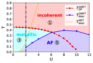
From the results in Fig. 4 (and more temperature points, not shown) one observes that, within DMFT, the onset of quasiparticle coherence associated with the crossover from the high- incoherent regime into the lower- metallic regime (regime ① to regime ② in Fig. 2) occurs at . This is in reasonable agreement with the QP coherence scale at the node from our benchmark calculations , but somewhat higher than the antinodal value , again due to the lack of momentum dependence of the self-energy, which is essential to account for nodal-antinodal differentiation. We have calculated the quasiparticle coherence temperature within DMFT as a function of coupling , and display the result in Fig. 6 (red line in upper panel). As expected, this scale decreases as the coupling is increased.
III.2 Crossover scales: the DMFT viewpoint
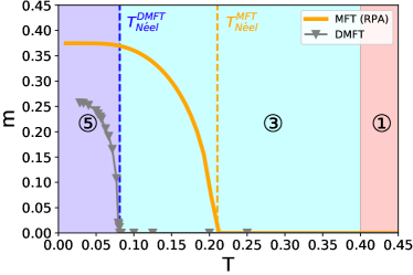
When used as an approximation for the two-dimensional half-filled Hubbard model of interest here, DMFT yields a symmetry breaking phase transition into an insulating phase with antiferromagnetic (AF) long-range order at finite temperatures for any value of . This is expected because DMFT does not take into account spatial fluctuations which destroy finite-T AF ordering in two dimensions (and, hence, does not satisfy the Mermin-Wagner theorem Mermin and Wagner (1966); Hohenberg (1967)). The Néel temperature obtained within DMFT is displayed in Fig. 6 as a function of (blue curve in upper panel), as well as the corresponding staggered magnetization as a function of temperature (lower panel). As expected, the Néel temperature displays a maximum, which signals the crossover between the weak-coupling regime in which the Néel temperature and magnetization are exponentially small, and the strong coupling regime. For very large , the charge gap is of order and the magnetization saturates. In that regime, for , spin degrees of freedom are described by an effective Heisenberg model with superexchange , and the DMFT Néel temperature is proportional to . For reference, we also display in Fig. 6 the result of the standard static mean-field theory (i.e. the Hartree mean-field for the transition into the spin-density wave phase, denoted below by ‘MFT’). MFT considerably overestimates the Néel temperature as well as for most values of . This is particularly pronounced at large where static MFT does not correctly separate spin and charge degrees of freedom so that the ordering temperature incorrectly coincides with the charge gap ( at large ) (for a comparison of MFT and DMFT see Sangiovanni et al. (2006)).
The key observation is that, taken together, the DMFT quasiparticle coherence scale (red line in Fig. 6) and the DMFT Néel temperature (blue line) can be taken as semi-quantitative mean-field estimates for the crossover lines separating the different regimes discussed in Fig. 2 above. The DMFT quasiparticle coherence scale is an estimate for the crossover into the metallic regime ③ in Fig. 2 (with comparable within error bars to the nodal value from our benchmark, while the antinodal one is about smaller). In turn, since in this weak-coupling regime the insulating gap is associated with magnetic quasi-long range order, the DMFT Néel temperature is an estimate for the onset of the insulating behavior - regime ⑤ in Fig. 2. Note that , compared to while is about smaller.
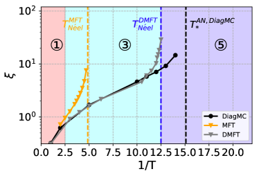
The magnetic correlation length can be calculated within both MFT and DMFT. In both cases this is achieved by the appropriate Bethe-Salpeter equations for the correlation function: with a static vertex equal to the bare within MFT (the calculation then reduces to the random phase approximation, RPA), and with a fully frequency-dependent but spatially local vertex within DMFT, see (Georges et al., 1996). It is often overlooked that mean-field methods (MFT or DMFT) provide us with a determination of correlation functions and indeed it naively appears as somewhat paradoxical that spatially dependent correlation functions can be obtained from a mean-field ansatz which is local at the one-particle level. This is actually a classic question in statistical mechanics, whose resolution lies in a careful interpretation of linear-response theory Parisi (1998). The mean-field correlation lengths are displayed in Fig. 7 in comparison to the DiagMC benchmark. It is apparent that the DMFT correlation length is in excellent agreement with the benchmark down to . The figure also clearly illustrates the connection between long-range magnetic correlations and insulating behavior.
III.3 The insulating regime
We finally comment on the comparison between the DMFT self-energies and the true solution in the low- insulating regime. Within DMFT, the insulating gap in this weak-coupling regime corresponds to a Slater mechanism associated with AF long-range order Slater (1951). It is associated with spin polarization and a non-zero value of the real part of the self-energy such that the quasiparticle equation has solutions only for outside the gap. The low-frequency behavior of the DMFT self-energy is non-singular, and in particular it has (using also particle-hole symmetry) a spin-independent linear term , corresponding to on the real frequency axis, which is similar in structure in the metallic phase and in the AF-ordered insulating phase. This is clearly apparent in Fig. 4. In contrast, because a spin polarization is absent at any non-zero in the true solution, the self-energy must be much more singular at low frequencies to open the insulating gap, as becomes clear from Fig. 3 and Fig. 4. The precise nature of this singularity is discussed in Sec. VII. At , however, the model does order and the general structure of the self-energy is expected to be similar to the Slater (and DMFT) one discussed above.
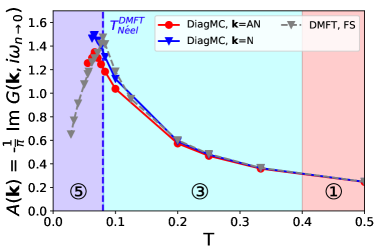
We finally display in Fig. 8 the value of the spectral function extrapolated to zero frequency, as obtained from DMFT as well as from the DiagMC benchmark at the node and antinode. Interestingly, there is rather good agreement between these different methods for this quantity, despite the different low-frequency behavior of the self-energy. In particular, we note that the crossover into the insulating regime is very sharp when seen from this physical observable, which is rather well approximated by the DMFT solution that has long range order in the insulating regime and hence displays a singularity at the Néel temperature. Detailed analysis close to the crossover temperature would of course reveal differences.
Summarizing, we see that DMFT provides a reasonable approximate description of the key crossovers encountered as a function of temperature. As a mean-field theory, it of course mimicks the crossover into an insulating phase with a large AF correlation length as a phase transition into a phase with long-range AF order. Including fluctuations beyond DMFT is therefore especially crucial in two dimensions, in which long-range order exists only at . This is the purpose of the cluster and diagrammatic (vertex-based) extensions of DMFT discussed in the following sections.
IV Including fluctuations beyond mean-field: single-particle properties
In this section, we show how the inclusion of (non-Gaussian bosonic) spatial fluctuations influences the one-particle properties (self-energies) beyond the mean field picture. This can be achieved by several methods: cluster extensions (dynamical cluster approximation DCA, cellular DMFT CDMFT, Sec. IV.1), and diagrammatic extensions of DMFT (Sec. IV.2) as well as with other approaches (Sec. IV.3). In this section, the results for the self-energy are presented and compared to the exact (benchmark) methods.
IV.1 Cluster extensions of DMFT: DCA and CDMFT
Quantum cluster methods Maier et al. (2005a) are quite natural extensions of DMFT in which the non-local components of the self-energy are computed by considering a cluster of sites self-consistently embedded in the lattice. This provides a controlled sequence of approximations which converge to the exact result when . Depending on the regime of parameters, convergence in this asymptotic limit may or may not be attained in practice however.
There are several flavors available within the broad family of quantum cluster theories, depending on how exactly the interacting cluster is described and how the embedding is performed. First we consider the dynamical cluster approximation (DCA, Hettler et al. (1998, 2000); Aryanpour et al. (2002)), where the Brillouin zone is paved with patches, and the self-energy is approximated as a piece-wise constant function over these patches whose components are calculated from a cluster of sites with periodic boundary conditions, hence defining the discrete momenta associated with each patch. For methodological details see Maier et al. (2005a) and App. D.5.
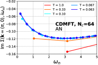
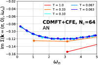
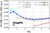
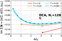
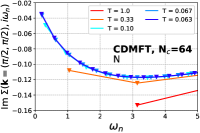
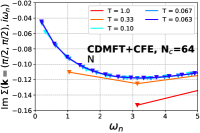
Fig. 9 (left) shows the self-energy on the Matsubara axis of a DCA calculation with N momentum patches for several temperatures and the benchmark DiagMC data as reference. For these calculations symmetry breaking to an AF long-range ordered phase was not allowed. We see that the improvement brought over single-site DMFT by these calculations is that the momentum-dependence of the quasiparticle coherence scale along the Fermi surface and nodal-antinodal differentiation is quantitatively reproduced (regimes ①-③).
However, the (non-magnetic) DCA with N is not able to open the pseudogap at low temperatures (shown in Fig. 9 until , i.e. ). The reason for this failure is easily understood by noting that the correlation length, previously displayed in Fig. 7, is lattice sites at the lowest T available () and even larger at lower T. A periodic cluster of finite size cannot resolve a correlation length larger than which is for . From this argument, one would expect that a cluster of order sites would be required to capture the opening of the insulating pseudogap with DCA in the case at hand. As discussed in Appendix D.5, this is beyond practical reach of the algorithm that we use here in the context of DCA.
A different strategy in the family of cluster extensions of DMFT is to consider a real-space embedding and hence a cluster with open boundary conditions, as in the cellular DMFT (CDMFT) approach Lichtenstein and Katsnelson (2000); Kotliar et al. (2001). Fig. 9 also displays data from CDMFT with . As apparent from these data, the real-space embedding method again captures the momentum differentiation of the coherence scale, but fails in opening the pseudogap for the same reasons as DCA (). From a quantitative perspective, a recently introduced extrapolation scheme (center focused extrapolation, CDMFT+CFE Klett et al. (2020), App. D.6) improves the comparison with the benchmark, however for the case also fails to open a gap. Hence, the size of the clusters has to be increased much beyond the values of Nc considered here in order to reproduce the pseudogap at this small interactions strength (see also Šimkovic et al. (2020)).
Summarizing, we conclude that extensions of DMFT based on cluster embedding methods succeed in reproducing the momentum dependence of the quasiparticle coherence scale (nodal-antinodal differentiation) in the metallic regime, but that much larger cluster sizes would be necessary in order to capture the opening of the insulating pseudogap, due to the very large correlation length in this weak coupling regime. Cluster embedding approaches perform much better in regimes with a smaller correlation length, such as larger values of (i.e. in the strong coupling regime) Rohringer et al. (2011) or (disregarding the sign-problem) when doping away from half-filling, as documented by the success of these methods in capturing the strong coupling pseudogap of the doped Hubbard model Gull et al. (2008a, 2009, 2010, 2013); Parcollet et al. (2004); Macridin et al. (2006); Tremblay et al. (2006); Sénéchal and Tremblay (2004); Haule and Kotliar (2007); Park et al. (2008); Ferrero et al. (2009a, b); Werner et al. (2009); Sordi et al. (2012a, b, 2013); Gunnarsson et al. (2015); Wu et al. (2018); Scheurer et al. (2018); Reymbaut et al. (2019).
Let us also note here that, analogously to what was done with DMFT in Fig. 8, allowing for AF order within these cluster methods - and hence mimicking the large correlation length regime as an ordered state - would most likely improve the agreement, see also Fratino et al. (2017). We do not attempt this here - see however Sec. VI for additional information about ordering within CDMFT.
IV.2 DA, TRILEX, and dual fermions/bosons
In view of the limitations of cluster embedding theories for this weak coupling regime, we now turn to an alternative way of treating long-ranged correlations more efficiently here, namely diagrammatic extensions of DMFT.
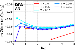
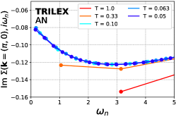
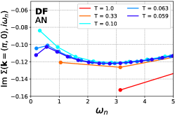
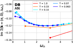
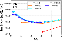
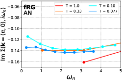
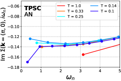
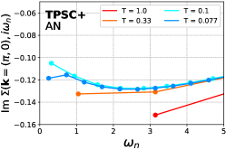
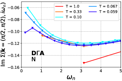
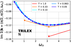
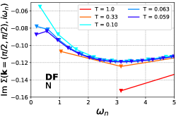
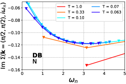
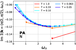
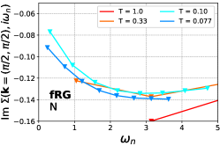
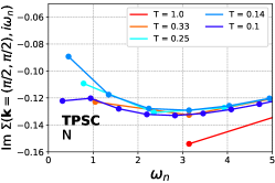
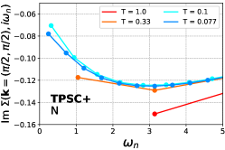
We display in Fig. 10 the results of several such diagrammatic extensions for the frequency-dependence of the self-energy at the antinode at different temperatures (apart from the diagrammatic extensions of DMFT also other approximation methods are considered there, see next subsection). Fig. 11 displays the results for the nodal point. Please note that the lowest temperature displayed is not always the same for the different methods, and it is useful to refer to Table 1 as a reminder of the important crossover scales. For the sake of comparison, the first panel shows again the data from the DiagMC benchmark.
We observe that all of the diagrammatic extensions of DMFT presented here [ladder-DA with a Moriya -correction in the spin channel (App. D.7), TRILEX (App. D.8), ladder DF (App. D.9) and single-shot DB (please note that, in the absence of the nonlocal interaction, the fully self-consistent DB theory would coincide with the DF approach when the bosonic hybridization function is discarded, see App. D.10)] are able to correctly reproduce the crossover from the incoherent to the metallic regime. Indeed, all methods display incoherent behavior (region ①) at high temperatures, before the onset of quasiparticles becomes visible first for the nodal point (region ②) and then, at lower temperatures, for the antinode (region ③). The temperatures of this onset , if at all, only slightly deviate from each other and the benchmarks within the numerical accuracy.
Larger deviations, both on a qualitative and quantitative level become visible, however, when lowering the temperature into the insulating pseudogap regime associated with growing magnetic correlations. Let us remind the reader that this crossover is signalled by a second change of slope in the self-energies - first at the antinode (region ④) and then at the node (region ⑤) - corresponding to a scattering rate that grows upon cooling.
Whereas DA and DF correctly reproduce these crossovers into the pseudogap regime, TRILEX does not exhibit these changes of slope, down to the lowest temperatures where we could converge the method. The DF method also succeeds rather quantitatively, both at the node and antinode, while the DB method appears to perform better at the antinode than at the node (but does not open the gap at the accessible temperatures). From a more quantitative point of view, DF and DB slightly underestimate the scattering rate at the node with respect to DiagMC whereas DA seems to slightly overestimate the scattering rate at the antinode and simultaneously exhibits a slightly lower than the benchmark.
Summarizing, we conclude that among the diagrammatic extensions of DMFT presented here, the D and the DF method appear to be best at capturing the different crossover regimes for the self-energy. In terms of the practical ability of performing calculations in this parameter regime, we must point out that all methods suffer from convergence problems when going down to lower and lower temperatures. The reason for these problems varies from method to method. For the benchmark methods: in DiagMC the series cannot be summed at low- and the DQMC suffers from the exponentially growing correlation length for . In the case of the DA (), lower temperatures can be reached if one is able to converge in the internal momentum grids. The same is true for TRILEX (), DF () and DB (). Please also note that within DiagMC the lowest reachable temperature is different for node and antinode ( vs. ).
IV.3 Other approaches: TPSC, TPSC+, fRG, PA
Figs. 10 and 11 also show results for three other approaches: TPSC/TPSC+, fRG and the parquet approximation (PA). Like the diagrammatic extensions of DMFT, all of them are able to reproduce the two distinct quasiparticle coherence scales at the node and antinode. However, there are significant deviations from the benchmark regarding the onset of the insulating pseudogap behavior.
TPSC is one of the first methods in which a detailed understanding of the mechanism responsible for the weak-coupling pseudogap was achieved early on (see Refs. Vilk (1995); Vilk and Tremblay (1996, 1997) and Sec. VII). As seen from Figs. 10 and 11, the change of slope in the self energies associated with the pseudogap opening is indeed qualitatively captured by TPSC, but the onset temperatures are severely overestimated. As discussed in Sec. VI, this is due to an overestimation of spin fluctuations in this method. A recent improvement of the method, TPSC+ Wang et al. , leads to a definite improvement in this respect as shown on the figures. TPSC+ partially feeds back the self-energy into the fluctuation propagators, mimicking frequency-dependent vertex corrections.
The PA appears to eventually capture insulating behavior at the antinode, although at lower temperatures in comparison to DiagMC, but doesn’t open a pseudogap at the node at this temperature.
The fRG calculations are possible only down to a “pseudocritical” temperature scale at which the running coupling constants diverge (see also the discussion in Ref. Hille et al. (2020b)). Down to this temperature, however, fRG is in qualitative agreement with the benchmark and shows a non-metallic behavior at the antinode (regime ④).
V Double occupancy and Pomeranchuk effect
In view of its physical significance discussed below, we present in this section the temperature-dependence of the double occupancy:
| (3) |
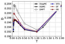
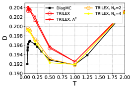
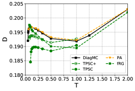
It is displayed as a function of temperature in Fig. 12, as obtained from different methods. We see (left panel, DQMC and DiagMC benchmarks) that three regimes are found: at high (down to about ) decreases upon cooling and then reaches a minimum, at intermediate temperatures actually increases upon cooling and, finally, sharply drops when entering the gapped regime. The high regime is expected and easy to understand: as is raised, an increasing number of high-energy doubly occupied configurations are thermally populated. This is apparent from the simple expression of in the atomic (zero hopping) limit:
| (4) |
which approaches for , i.e. at very high temperatures or, alternatively, in the non-interacting limit. The intermediate regime in which increases upon cooling is more interesting - note that this regime includes in particular large parts of the metallic region ③. As observed early on in Ref. (Georges and Krauth, 1993), this apparently counter-intuitive non-monotonic behaviour of can be understood qualitatively from entropy considerations. Observing that the entropy is obtained from the free energy as and that , one obtains the thermodynamic Maxwell relation:
| (5) |
Increasing at fixed temperature in the metallic regime leads to an increase in entropy. Indeed, in this regime, the entropy is linear in with a slope related to the effective mass which grows as is increased. Hence, the right-hand side of Eq. (5) is negative and thus must increase upon cooling/decrease upon heating in this regime. This is the same phenomenon as the famous ‘Pomeranchuk effect’ in liquid 3He (Clausius-Clapeyron equation): upon heating the system, a tendency to increased localization (smaller ) is found, because localization leads to a higher (spin) entropy and is thus favorable thermodynamically (until thermal population of doubly occupied sites kicks in at higher ). Note that the sign of also directly determines the shape of the isentropy lines in the plane, which are defined by and hence obey Werner et al. (2005); Daré et al. (2007):
| (6) |
with the specific heat per lattice site. Hence cooling can in principle be achieved by increasing the interaction strength adiabatically in the regime where , as initially suggested in Werner et al. (2005), further discussed in Daré et al. (2007), and experimentally realized in cold atomic systems with extended -symmetry Taie et al. (2012).
Finally, the low behaviour in which sharply decreases again upon cooling corresponds to temperatures around regime ④ in which the system behaves as an antiferromagnetc insulator. We note that the total energy of the Hubbard model is given by:
so that . The drop in can be understood from the fact that at small the crossover into the (Slater) antiferromagnetic correlation regime corresponds to a gain in potential energy Fratino et al. (2017); Schäfer et al. (2015a); Rohringer and Toschi (2016). It was shown in Ref. Fratino et al. (2017) that at strong coupling, in contrast, increases when entering the (Heisenberg) antiferromagnetic correlations regime, corresponding to a gain in kinetic energy.
We see (left panel of Fig. 12) that DMFT reproduces all three regimes qualitatively, but overestimates the amplitude of the ‘Pomeranchuk effect’ by approximately a factor of two, as discussed in Ref. Daré et al. (2007). The reason is that the spin entropy in the localized state at high- is overestimated in DMFT, due to its neglect of spatial correlations. Obviously, in DMFT, the sharp drop at low corresponds to the phase transition into an ordered phase - a mean-field description of the actual crossover (see above). This can also be seen as an increase of the magnetic local moment, since via the double occupancy is related to the increase of AF correlations.
All the methods displayed in Fig. 12 qualitatively reproduce the non-monotonous behaviour of but the sharp drop at low is, as expected, only present in the methods which can describe the low antiferromagnetic insulator regime. It is, for this reason, absent in the TRILEX based methods for the range of temperatures studied (middle panel). Single-site TRILEX also overestimates significantly, but cluster extensions of TRILEX are closer to the benchmark at intermediate . DF similarly overestimates the double occupancy. For details, including differences between different variants of these ‘dual’ methods, see the discussion about self-consistency in App. D.10. fRG qualitatively captures the Pomeranchuk effect. In the present implementation, however, it does not display a drop at low temperatures.
In contrast, DA and DB (single-shot) follow the benchmark quite accurately. Also, the parquet approximation (PA) appears to capture all three described regimes, while TPSC and TPSC+ qualitatively predict the correct physical picture albeit less accurate quantitatively than PA in comparison to the benchmarks.
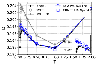
The above results suggest that long-range magnetic correlations are the cause of the downturn of the double occupancy at low temperatures. To further establish this point, we display in Fig. 13 the double occupancy vs. temperature calculated with DMFT by either constraining the solution to remain paramagnetic or allowing for the solution with long-range AF order (which is the lower-energy stable solution at low- within DMFT). One sees that only the latter displays the downturn, emphasizing that the AF ordered solution, despite violating Mermin-Wagner theorem, is a better approximation to thermodynamic quantities in a regime where the correlation length is large. We also display in Fig. 13 the results obtained with DCA and CDMFT, restricted to the PM solution. In that case, as expected, the downturn is not reproduced, since the cluster sizes investigated here are too small as compared to the correlation length (see also the discussion in Sec. IV.1).
We end this section with a technical remark on the actual calculation of in the investigated methods. In DQMC and DiagMC can be directly calculated as an equal-time correlation function. For the other methods the calculation of the double occupancy is possible either via the (lattice) Green’s function and self-energy, utilizing the equation of motion technique based on the Galitskii-Migdal formula Galitskii and Migdal (1958):
| (8) |
(used in the DA, DF, PA and TPSC/TPSC+, for details on the latter see App. D.11) or, when allowed by the algorithm used for the impurity solver, from a direct computation on the impurity (for DMFT, its cluster extensions and TRILEX, see also van Loon et al. (2016)). The DB result was obtained via the local part of the lattice susceptibility as discussed in Ref. van Loon et al. (2016). For a comparison to self-consistent DB we refer to App. D.10. For details on the calculation of in fRG we refer to App. D.12. We note in passing that, when applying Eq. (8), treating the high frequency tails is very important to obtain accurate results.
VI Including fluctuations beyond mean-field: magnetic correlations
In this section, we turn to two-particle correlation functions and compare the different methods for two important observables probing the magnetic correlations: the static antiferromagnetic spin susceptibility and the magnetic correlation length .
VI.1 Antiferromagnetic static spin susceptibility
The spin susceptibility (or spin correlation function) is given by:
| (9) |
where we define here
| (10) |
and . Note that we omit for simplicity an additional prefactor of for the spin operator and that at half-filling in the paramagnetic phase ().
The temperature dependence of the static spin susceptibility
is of particular interest for the case of the half-filled Hubbard model on the square lattice, as the perfect nesting (see Fig. 1) leads to a strong enhancement at .
The temperature dependence of reflects the increasing
dominance of antiferromagnetic spin fluctuations upon cooling.
One starts at high with almost independent fluctuating moments and a Curie law
(bosonic mean-field behavior). Approaching the ground-state with antiferromagnetic long-range
order, the range of spin correlations grows and nonlocal spin fluctuations in the paramagnetic phase
(antiferromagnetic paramagnons) develop.
At low-, a regime with an exponentially growing correlation length is found (see below).
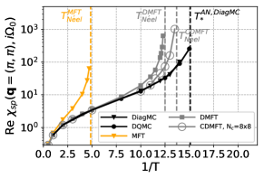
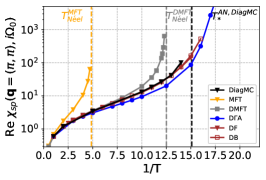
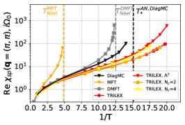
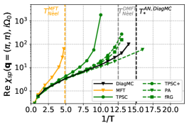
Figs. 14 and 15 displays for various methods as a function of (inverse) temperatures on a logarithmic scale. We start our analysis with Fig. 14. As already described in the with the mean-field picture in Sec. III both MFT (, orange triangles) and DMFT (, gray squares), due to their mean-field nature,
incorrectly predict finite Néel temperatures: the crossover is mimicked as a true (continuous) phase transition (left panel). The thermodynamic transition manifests itself as a divergence of the susceptibility at the corresponding wave vector.
Of course, the Mermin-Wagner theorem prohibits finite temperature ordering in 2D, which is reflected in the data of both benchmark methods DiagMC (black triangles) and DQMC (black circles), whose susceptibilities do not diverge at finite . Rather, after following the mean-field curves at high temperatures, the benchmark data enter an intermediate regime in which appears to increase approximately exponentially. This regime largely coincides with the metallic regime ③, eventually crossing over into a second exponential regime at low- (see also Sec. VI.3), which sets in at a temperature close to the DMFT Néel ordering.
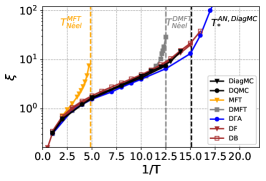
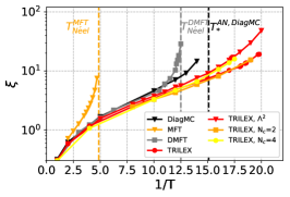
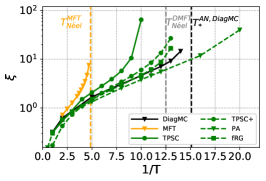
This low exponential regime is to be expected, since there, the charge degrees of freedom are frozen out by the gap and the system enters the insulating regime ⑤, as indicated by the black dashed line . In this regime, the effective spin dynamics is expected to be described by a non-linear sigma model and this exponential growth is typical of the lower critical dimension Chakravarty et al. (1988, 1989); Vilk and Tremblay (1997); Borejsza and Dupuis (2003, 2004). The first exponential observed in the metallic regime is more surprising and will be discussed in more details below. Let us stress that, due to the reasons already mentioned for single-particle quantities, both benchmark methods are limited in terms of the temperatures they can reach (). Please note that the lowest reachable temperature differs from the one for the self-energy.
The inclusion of short-range correlations with CDMFT leads to (i) a quantitative agreement with the benchmark until and (ii) only a slight drop of the Néel temperature in comparison to DMFT, to . In principle, as the cluster extensions of DMFT are controlled methods, the Mermin-Wagner theorem is restored in the infinite cluster size limit. However, this restoration has been shown to be logarithmic in the strong-coupling regime Maier et al. (2005b), which is in agreement with this very small change in (see also Klett et al. (2020)).
Turning to the diagrammatic extensions of DMFT, in the left panel of Fig. 15 one can see that DA (left panel), which respects the Mermin-Wagner theorem Toschi et al. (2007); Katanin et al. (2009); Rohringer and Toschi (2016, 2020), captures well the different regimes of the benchmark (Curie law at high temperatures and the two exponential regimes). The small quantitative underestimation observed here may potentially be cured by an improved version of the Moriya -correction Rohringer and Toschi (2016) or a more thorough treatment of the asymptotics of the vertex function as a function of frequency Wentzell et al. (2020); Kaufmann et al. (2017); Katanin (2020). DF and single-shot DB agree well with the benchmark where the algorithm can be reliably converged.
In the case of TRILEX (central panel) we present results for different variants of the method, all of which seem to capture a low temperature exponential scaling, however, with different degrees of accuracy: whereas single-site TRILEX (red circles, solid line) and cluster TRILEX with two cluster sites (TRILEX N, orange squares) largely underestimate the values of the susceptibility, the result is significantly improved by increasing the cluster size to four (TRILEX N, yellow circles). Remarkably, the TRILEX variant with the electron-boson vertex inserted on both sides (TRILEX , red triangles, see App. D.8) seems to be on top of the cluster N results. Investigating how these values eventually converge to the exact results with is left to future studies.
We finally turn to the other methods (right panel): Both PA and fRG capture quantitatively the high- Curie regime. The PA appears to systematically underestimate from on, whereas fRG is overestimating it. Let us just comment here that although the presented fRG scheme does not fulfill the Mermin-Wagner theorem, its recent multiloop extension Kugler and von Delft (2018a, b); Hille et al. (2020a) and the PA does Bickers and Scalapino (1992); Eckhardt et al. (2020) (see also Baier et al. (2004)). Both TPSC and TPSC+ are in agreement with the benchmarks at high temperature, but, as already mentioned in the previous section about the self-energy, the spin fluctuation intensity is significantly overestimated in TPSC with respect to the benchmark (right panel). This overestimation is improved again in the TPSC+.
Our results also demonstrate that, remarkably, neither the fact that the Mermin-Wagner theorem is respected by a theory nor that a theory uses self-consistent interacting Green functions, guarantees a quantitatively better result, as can be inferred by a comparison of the TPSC or PA result with the benchmark, respectively.
VI.2 Magnetic correlation length
The spatial range of antiferromagnetic spin correlations can be quantified by the magnetic correlation length , which in practice can be extracted by a fitting procedure using the Ornstein-Zernike (OZ) form of the bosonic propagator Ornstein and Zernike (1916):
| (11) |
The results presented in this section were obtained using a slightly modified form of the OZ expression, appropriate for a model on a lattice, as described in App. A. Note that we neglect (small) deviations from the OZ form beyond mean-field. Within the OZ form, the AF static susceptibility discussed previously obeys: .
Fig. 16 shows the correlation length obtained via such a fitting procedure applied to the susceptibility data from the different methods. One can immediately see that the curves are, to a large extent, qualitatively similar to the susceptibility curves of Fig. 15. Interestingly, the intermediate- exponential behaviour in the metallic regime is clearly visible in the DiagMC benchmark data. The lowest- exponential regime in the insulator is hard to reach with DiagMC, but is obtained in DA (and, less clearly, in PA and TRILEX) which can be used down to lower temperature than the benchmark methods. We note, however, that sizeable quantitative differences do exist between the different methods at low-, and hence we conclude that the precise determination of the correlation length in the low- regime, where it becomes exponentially large, is a challenge for all state of the art computational methods currently available.
VI.3 The three regimes of magnetic correlations
Summarizing, we observe three successive regimes for magnetic correlations as the temperature is lowered. At high- (), a Curie mean-field behaviour is found with a small correlation length (), and all methods (except static MFT) are basically in quantitative agreement in this regime. At intermediate temperatures , we find a correlation length that appears to increase exponentially to a good approximation, with values reaching . This is somewhat surprising since this regime is metallic with quasiparticles that become more coherent as temperature is lowered, at least in the nodal region. We discuss further the physical significance of this finding in Sec. VII by comparing to spin-fluctuation theories. All methods reproduce this intermediate exponential regime qualitatively. On the quantitative level, excellent agreement is found between the benchmark DiagMC and especially DF and DB throughout this regime. We also note very good agreement for the determination of the correlation length with DMFT and TPSC+ down to . Most other methods (DA, the various variants of TRILEX and the PA) also provide a satisfactory determination of the susceptibility and correlation length in this intermediate regime.
The low-temperature insulating regime can hardly be probed with current state of the art benchmark methods. The DA results down to are consistent with the exponential growth of the correlation length Schäfer et al. (2015a); Rohringer and Toschi (2016), expected from the low-energy description of the spin degrees of freedom by a non-linear sigma model once a charge (pseudo)gap opens up. We note significant discrepancies between the different approximate methods available in this regime however. The growth rate of this exponential regime appears to be different (and faster) than the one in the intermediate- metallic regime, a finding which will have to be confirmed in future work by exact computational methods when they become capable of reaching lower temperatures.
VII Insights into the nature and role of spin fluctuations
In this section, we provide understanding into the physical nature of the different regimes highlighted above, especially the metallic regime and the (pseudo)gapped insulating regime. We focus in particular on the nature and role of spin fluctuations. We explore whether spin fluctuation theory of the weak-coupling type is able to describe qualitatively the various regimes: this analysis also provides analytical insights into the physics of these different regimes. We focus in particular on the following key questions:
-
(i)
What is the physical mechanism for the opening of the pseudogap at low temperature?
-
(ii)
What are the implications of the growing antiferromagnetic correlation length upon cooling for the coherence of quasiparticles in the metallic regime?
-
(iii)
To what extent can this metallic regime be characterized as a Fermi liquid?
VII.1 Weak-coupling spin fluctuation theory
In this subsection, we interrogate weak-coupling spin-fluctuation theory and ask whether it provides a satisfactory description of the behaviour of the self-energy, at least on a qualitative level, in the different regimes of temperature. This will also provide guidance throughout the rest of this section in identifying which fluctuations contribute most to the self-energy.
In the simplest version of spin fluctuation theory the self-energy can be expressed as (omitting the Hartree term):
In this expression, is the momentum- and frequency-dependent spin susceptibility and is the (lattice) Green function. In the following we always choose to be the non-interacting Green function, see the end of Sec. VII.2 for comments about the drawbacks of self-consistent schemes.
The coupling constant in Eq. (VII.1) characterizes the coupling between electrons and the spin collective modes. It is renormalized as compared to its bare value as increases. In the following, we are more interested in asking whether weak coupling spin fluctuation theory qualitatively captures the different regimes than in quantitative statements. However, when a comparison is attempted, a value of has to be chosen. For example, in the version of TPSC considered in the present article, is given by (focusing on the spin channel only): , with . The factor ensures rotational invariance by properly accounting for the relative contributions of longitudinal and transverse spin fluctuations Moukouri et al. (2000), while the expression of is key to the TPSC scheme, see also App. D.11. In the following we shall, for simplicity, use when performing quantitative comparisons.
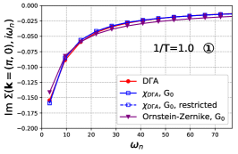
Fig. 17 presents a comparison between the DA results for the self-energy at the antinode and the spin-fluctuation expression Eq. (VII.1) in which different choices are made for the spin susceptibility . We perform the comparison using the susceptibility data from DA due to its good agreement with the benchmark, the availability of the -resolved susceptibility and its ability to enter the highly insulating regime ⑤. This comparison is performed for three different temperatures, corresponding to the incoherent regime ①, the metallic regime ③ and the pseudogapped insulating regime ⑤.
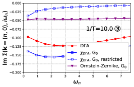
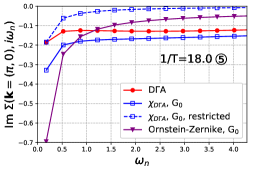
We begin the discussion with the result obtained by using the full (solid blue curve, square markers) DA susceptibility. We see that, at a qualitative level, the spin-fluctuation approximation succeeds in reproducing the characteristic low-frequency dependence of the self-energy associated with all three regimes. There is furthermore good quantitative agreement in the incoherent regime ①. With the chosen value of , the self-energy is overestimated in both the metallic and pseudogap regimes. Using together with the value of the double occupancy calculated in Fig. 12 largely remedies this overestimation for most of the metallic regime.
In order to better understand which spin fluctuations dominate the different regimes, we have also applied Eq. (VII.1) by restricting the integration over the momentum transfer to the vicinity of the antiferromagnetic wave vector according to (dashed blue curves in Fig. 17). We see that in the pseudogap regime ⑤ the qualitative frequency dependence of the antinodal self-energy is not modified by this restriction (although obviously, as a result of the restriction in the integration, the self-energy is underestimated by an amount which is approximately frequency independent). This indicates that, in this regime, the self-energy is indeed dominated by the antiferromagnetic collective modes associated with the vicinity of . In contrast, a completely different situation is found in the metallic regime ③: restricting the momentum sum to the vicinity of yields a spin-fluctuation self-energy which has a qualitatively different frequency dependence than the actual one, inconsistent with the properties of a metal (and actually closer to the shape associated with a pseudogap). It also underestimates the overall order of magnitude of the self-energy by more than a factor of four. We thus conclude that the single-particle properties in the metallic regime are not controlled only by the spin fluctuations associated with the antiferromagnetic wave vector: taking into account spin fluctuations at other wave vectors is crucial. We will come back in detail to this observation in Sec. VII.3. We finally note that the incoherent regime is not affected by the momentum restriction, simply because the correlation length is so small there that our criterion on the transfer momentum actually does not restrict the integration domain significantly.
Finally, we consider whether the spin susceptibility in Eq. (VII.1) can be approximated, as often done in spin fluctuation theories, by an Ornstein-Zernike form emphasizing long-wavelength antiferromagnetic fluctuations:
| (13) |
As detailed in App. A, we use a lattice generalization of this expression and perform a fit of the momentum and frequency dependence of the DA susceptibility in order to determine the amplitude , correlation length (Sec. VI) and Landau damping coefficient as a function of temperature. The antinodal self-energy obtained by inserting expression (13) into the spin-fluctuation expression (VII.1) is displayed in Fig. 17 (purple data points). This approximation is quantitatively accurate in the high-temperature incoherent regime. It captures qualitatively the characteristic frequency dependence of a pseudogap in the low-temperature regime, as also detailed analytically in the following section, but considerably overestimates its magnitude. In contrast, in the metallic regime, it fails quite severely both qualitatively and quantitatively, indicating that the Ornstein-Zernike approximation fails to capture important spectral weight in at far from which is crucial in the metallic regime as emphasized above and further detailed in Sec. VII.3.
VII.2 Analytical insights into the pseudogap insulating regime
We provide here some analytical insights into the low- pseudogap regime, based on the weak coupling spin fluctuation theory and the Ornstein-Zernike approximation for the spin susceptibility in Eq. (13). As seen above, these approximations are qualitatively reasonable (although not quantitatively accurate) in this regime. For pioneering works on the formation of a pseudogap due to antiferromagnetic correlation, see Refs. Vilk and Tremblay (1997) and Borejsza and Dupuis (2004). In the latter, the authors focused on orientational fluctuations of the antiferromagnetic order described by a non-linear sigma model and, expressing the physical electron as a product of a Schwinger boson and an auxiliary fermion, were able to describe the crossover from a weak-coupling pseudogap in the Slater regime to a strong-coupling insulating gap in the Mott-Hubbard regime.
In this ‘renormalized classical’ regime, only the lowest Matsubara frequency needs to be retained in Eq. (VII.1) leading to Vilk and Tremblay (1996, 1997); Wu et al. (2018):
| (14) |
In this expression, the prefactor of the spin susceptibility has been combined with and numerical prefactors to yield a coupling with the dimension of an energy. In Eq. (14), only the dominant term has been retained, is a point on the Fermi surface away from the van Hove singularity (i.e. from the antinode) so that the Fermi velocity is non-vanishing, and designates the important low-energy scale:
| (15) |
which explicitly depends on the Fermi velocity (i.e. ). In the last expression, we have postulated an exponential growth of the correlation length, characteristic of the low- gapped regime, with as the spin stiffness. Expression (14) has the following behaviour at low and high (imaginary) frequency:
| (16) | |||||
| (17) |
These expressions shed light on the dependence of the self-energy on Matsubara frequency reported above in the low- regime. The lowest Matsubara frequency in this regime is always larger than the tiny low-energy scale : in fact the condition defines the range of low temperatures in which the insulating/pseudogap behaviour is observed Vilk and Tremblay (1996, 1997). In this regime, the Matsubara frequency self-energy seemingly displays a downwards divergent behaviour as in Eq. (16). However, if a calculation for low- was possible, it would actually display a saturation to a finite value as in Eq. (17).
For completeness, we discuss the implications of this expression for the low-frequency spectral function and self-energy on the real frequency axis. Analytically continuing the above expression yields (for ):
| (18) | |||||
| (19) |
with the following asymptotic forms:
| (20) | |||||
| (21) |
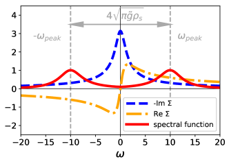
with a slope obviously having a sign opposite to that of a Fermi liquid (‘’). The corresponding self-energy and spectral function on the Fermi surface are plotted in Fig. 18. The two prominent peaks at the edge of the pseudogap in the spectral function can be understood by using the asymptotic form of for in the quasiparticle equation . We see that the poles of the Green function are located at a frequency such that . The dominant term on the r.h.s. of this equation is from , and we finally obtain the locations of the main peaks at:
| (22) |
where the corrections are linear in temperature. Hence, the location of these peaks become temperature-independent in the low- limit. As these two peaks evolve continuously into the gap-edge peaks defining the single-particle excitations across the insulating gap due to long-range antiferromagnetic order. Note that, within mean-field theory the gap is given by with as the staggered magnetization, and that close to a quantum critical point the scaling indeed holds, establishing consistency with Eq. (22) (in the present case of additional logarithmic corrections intervene). Note that the above derivation of the pseudogap behaviour down to relies on the exponential growth of the correlation length and hence would not apply if the ground-state did not have long-range order. For an alternative approach based on thermal fluctuations starting from the ordered state, see Ref. Sedrakyan and Chubukov (2010).
The width of the AF insulating peaks Slater (1951); Borejsza and Dupuis (2003, 2004) are of order (for a DMFT analysis see also Sangiovanni et al. (2006)). It is furthermore interesting to understand the pseudogap regime in terms of lengths instead of the energy Vilk and Tremblay (1997). The one-particle thermal de Broglie wavelength determines the maximum distance over which an electron wave packet remains coherent despite thermal agitation. Eq. (21) shows that the imaginary part of the self-energy at zero frequency becomes very large when this length is smaller than the correlation length for spin fluctuations, leading to the decrease of spectral weight at zero frequency. For electrons in the pseudogap regime, the spins look ordered over the length where temperature does not destroy its coherence. This argument holds only in two dimensions. In higher dimensions, the phase space associated with the integration over wave vectors in Eq. (VII.1) diminishes the importance of long wavelength fluctuations Vilk and Tremblay (1997) for the self-energy. As is well known from DMFT, in infinite dimensions, the self-energy is not influenced by long-wavelength spin fluctuations Metzner and Vollhardt (1989); Georges and Kotliar (1992).
A similar analysis can be performed for Fermi surface points in the vicinity of a van Hove singularity, i.e. when . The expansion of the dispersion relation then is stopped only after the second order term, giving for after integration over
| Im | (23) | ||||
| (24) |
which yields logarithmic divergences. Even if these divergences could be cut off, for
| (25) |
so that the imaginary part of is now proportional to instead of (see also Vilk and Tremblay (1997); Vilk (1997); Rohringer and Toschi (2016), Lemay (2000); Zlatic (1997) for second order perturbation theory and Katanin et al. (2005) in the context of ferromagnetic fluctuations), i.e. way larger than for momenta away from van Hove points.
To conclude this subsection on the pseudogap insulating regime, we recall some findings and comment on the ability of the description of this regime in self-consistent theories. First we note, that if one uses (with a finite self-energy) instead of as fermionic propagator in Eq. (VII.1), one obtains Im , hence missing the exponential growth of Eqs. (17,25) Rohringer and Toschi (2016), see also Borejsza and Dupuis (2003).
On more general grounds, we note that the self-consistency at the level of vertex corrections should be consistent with the one of the Green function. This remark serves as a warning about imposing self-consistency solely over the Green function. When using approximate schemes which truncate perturbation theory or select a specific class of diagrams without taking vertex corrections into account in a consistent manner, self-consistency may lead to an incorrect physical description - especially in relation to the opening of insulating gaps. For an insightful discussion of these limitations of self-consistent perturbation theory, see Sec. 6.1 of Ref. Vilk and Tremblay (1997). Observations about the inadequacy of self-consistency in truncated perturbation theory approximations have previously been made also in other contexts, such as the GW approximation and DMFT where it is well-known that self-consistent perturbation theory truncated to second-order fails in yielding Hubbard bands and the opening of a Mott gap Georges and Kotliar (1992); Müller-Hartmann (1989); Ku and Eguiluz (2002); Delaney et al. (2004); Ku and Eguiluz (2004). An additional, however, completely different problem can arise when self-consistent theories (e.g. bold diagrammatic Monte Carlo Prokof’ev and Svistunov (2007); Deng et al. (2015)) are applied: due to the multivaluedness of the Luttinger-Ward functional Kozik et al. (2015); Stan et al. (2015); Vučičević et al. (2018); Rossi and Werner (2015); Kim and Sacksteder (2020), intimately related Gunnarsson et al. (2017) to divergences in vertex functions Schäfer et al. (2013); Janiš and Pokorný (2014); Schäfer et al. (2016b); Chalupa et al. (2018); Thunström et al. (2018); Springer et al. (2020); Reitner et al. (2020); Chalupa et al. (2021), the bold approaches may converge to an unphysical branch.
VII.3 Insights into the metallic regime
VII.3.1 Temperature dependence and characteristic scales
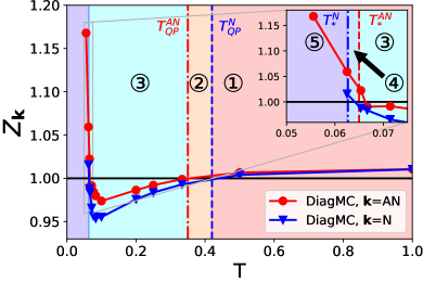
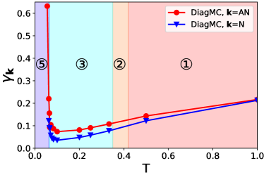
Finally, in this section, we provide insights into the physics of the metallic regime. We display in Fig. 19 the quantities
| (26) | |||||
| (27) |
as a function of temperature, at the nodal and antinodal points on the Fermi surface, obtained by a fit to the DiagMC self-energy on Matsubara frequencies. For the details about how these parameters are extracted, see App. B. For a Fermi liquid, would correspond to the quasiparticle spectral weight and to the inverse of the quasiparticle lifetime. We are dealing however with a perfectly nested system in which Fermi liquid behaviour does not strictly apply, and this interpretation has to be taken with care, as further discussed in Sec. VII.3.3. Indeed, we observe that at the nodal point follows an approximately -linear temperature dependence for . The antinodal value of is significantly larger, highlighting momentum differentiation.
The metallic regime ③ was conventionally defined above as the regime where the self-energy has a negative slope at low frequency, thus allowing to define a smaller than unity, as indicated on the upper panel of Fig. 19. From the -dependence of , we see that region ③ defined in this manner actually consists of two sub-regimes (see also Rohe and Honerkamp (2020); Afchain et al. (2005)): For (regime ③a covering most of region ③), the inverse quasiparticle lifetime decreases upon reducing , indicating an increase of quasiparticle coherence upon cooling (as characteristic of a metal). When cooling below a minimum of (and ) is found, below which the lifetime decreases upon cooling as a precursor of the pseudogap regime (regime ③b).
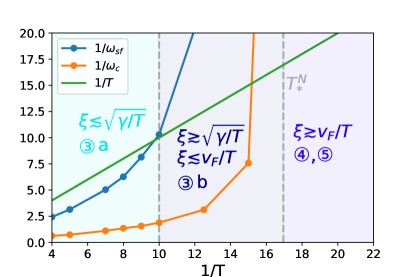
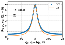
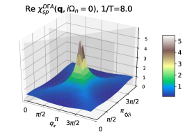

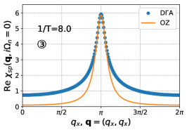
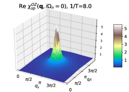
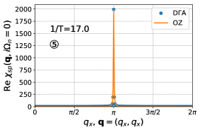
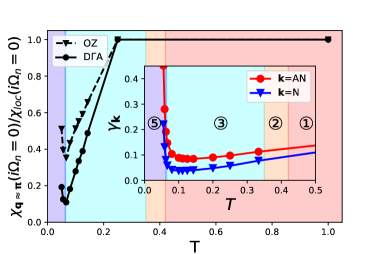
In order to rationalize these findings, we turn again to spin fluctuation theory, Eq. (VII.1). In contrast to the pseudogap regime, it is crucial here to perform the full convolution over all Matsubara frequencies. Using the spectral representation of , the single-particle scattering rate at zero frequency is obtained from Eq. (VII.1) as:
The key point here is to compare the width in frequency of the two factors entering this expression: and . The width of the former is of order temperature , while the width of the latter is set by Landau damping, as clear from the Ornstein-Zernike form Eq. (13) applicable close to the antiferromagnetic wavevector which reads for real frequencies:
| (29) |
This expression peaks at the characteristic spin fluctuation frequency:
| (30) |
Hence, for , only the low-frequency behaviour of matters in Eq. (VII.3.1). This analysis shows that, besides the scale which controls the pseudogap regime, the spin-fluctuation scale is important for the physics of the metallic regime (see Abanov et al. (2003) and references therein). In Fig. 20, we display these two scales as a function of temperature, with and determined from a fit to the DA susceptibility as described above and in App. A. We compare these two scales to temperature itself, and observe that this indeed defines three distinct regimes, which correspond to a very good approximation to the regimes observed in our numerical results, namely (note that ):
-
•
(): metallic regime ③a.
-
•
(, Vilk criterion): insulating pseudogap regime ④, ⑤.
-
•
(). In this narrow intermediate regime (, ③b) the pseudogap is not yet fully opened but the scattering rate no longer behaves as in a metal: it displays a minimum and increases at lower as the pseudogap regime is entered, as displayed in Fig. 19. We note in passing that the upper boundary of this regime coincides with the temperature at which the double occupancy displays a local maximum (see Fig. 12), corresponding to the onset temperature above which local magnetic moments are formed (see also Kim et al. (2020); Chalupa et al. (2021)). It also has corresponding signatures in other thermodynamic observables Kim et al. (2020).
VII.3.2 Which fluctuations dominate the metallic regime ?
Expression (VII.3.1) also allows to understand an important observation made in Sec. VII.1, namely that in the metallic regime the spin fluctuations contributing to the self-energy are not dominated only by the vicinity of the antiferromagnetic wave vector.
In order to further document and validate this point, we display in Fig. 21 a comparison between the momentum dependence of the spin susceptibility as obtained in DA and that of its Ornstein-Zernike fit (the latter privileges the vicinity of the antiferromagnetic wave vector). We see (left panel) that at which lies in the metallic regime, the OZ fit captures very poorly the momentum dependence of the susceptibility far from . In particular, the OZ fit misses the sizeable weight that is visible in the DA susceptibility along the diagonals . That weight comes from scattering associated with nesting vectors parallel to the antiferromagnetic zone boundaries, as is apparent already in second-order perturbation theory Lemay (2000). In contrast, the OZ form is much more accurate at lower temperatures when has grown to larger values and the system is in the pseudogap regime (right panel): indeed, the physics of the pseudogap is dominated by antiferromagnetic fluctuations (Sec. VII.2).
This is further documented in Fig. 22 which displays the ratio between the susceptibility integrated over a region of the order of around to its integral over the whole zone. It is seen that this ratio decreases as is lowered throughout the metallic regime, while it increases again in the pseudogap regime: hence a large fraction of the spectral weight is missed by focusing on the vicinity of in the metallic regime. Fig. 22 also shows that the OZ fit overestimates the relative spectral weight associated with the vicinity of the antiferromagnetic wave vector.
Using the expressions (VII.3.1) and (29), it can be shown that the contribution of the spin-fluctuations to the zero-frequency scattering rate on the FS (away from the van Hove point) behaves in the metallic regime as . As shown in Appendix A, the ratio decreases quickly upon cooling in this regime, which insures that this contribution to the scattering rate also decreases despite the fast increase of the correlation length. A similar remark applies to the local (momentum-integrated) scattering rate, for which this contribution can be estimated as (up to logarithmic terms). However, importantly, the local self-energy involves contributions from fluctuations at all wave-vectors, as already clear at the level of the spin-fluctuation approximation by integrating Eq. (VII.3.1) over . This explains why DMFT provides, in the metallic regime, an excellent approximation to the local component of the self-energy. In contrast, the DMFT approximation does not properly capture the contributions to the self-energy of fluctuations which are strongly peaked at a specific wave vector. For a plot of the (negative) imaginary part of the local self-energy extrapolated to zero Matsubara frequency a function of temperature we refer to Fig. 28 in App. A.
Summarizing, we have shown that a comparison of the two key energy scales and to temperature allows for a determination of the different physical regimes as a function of temperature, in excellent quantitative agreement with our numerical results. The momentum-differentiated metallic regime evolves at low- into a precursor regime of the pseudogap where the quasiparticle lifetime reaches a maximum. We have also shown that the metallic regime is not dominated by the spin fluctuations associated with only the antiferromagnetic wave vector, and explained why quasiparticles with a lifetime increasing upon cooling can coexist with antiferromagnetic fluctuations characterized by a correlation length which strongly increases (approximately exponentially).
VII.3.3 Perfect nesting and non-Fermi liquid behaviour
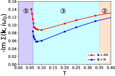
In the half-filled model with considered in this paper, we do not expect Fermi liquid behaviour to hold in the metallic phase because of perfect nesting. Indeed, the whole one-dimensional set of wave vectors with maps a point on the diamond-shaped Fermi surface onto another one. In this section, we briefly discuss whether our computations can detect hints of non-Fermi liquid behaviour, despite providing data restricted to imaginary (Matsubara) frequencies.
In a Fermi liquid, the self-energy takes the following form, when considered on the Fermi surface and at low frequency and temperature:
| (31) |
On the Matsubara axis, the r.h.s. of this expression reads . This contribution vanishes when considering the first Matsubara frequency . Hence, the temperature dependence of at the first Matsubara frequency is controlled by the dominant term with no quadratic correction of order : linear dependence of this quantity on temperature is a hallmark of Fermi liquid behaviour (‘first Matsubara frequency rule’, see Ref. Chubukov and Maslov (2012)). Fig. 23, displays the -dependence of this quantity as obtained from the benchmark DiagMC at both the nodal and antinodal points on the Fermi surface. We see visible deviation from linearity throughout the metallic regime, indeed hinting at a departure from Fermi liquid behavior. Further evidence for non-Fermi liquid behaviour is provided by the dependence on temperature of the parameters and obtained by a fit of the self-energy on Matsubara frequencies and displayed above on Fig. 19. Indeed, (i) does not stabilize to a T-independent value before the pseudogap kicks in, but rather slowly decreases throughout the metallic regime and (ii) the temperature dependence of is better described as -linear rather that quadratic like in a Fermi liquid. Further details about the proper interpretation of the Matsubara fitted parameters and when Fermi liquid behaviour does not apply are given in Appendices B and C.
The breakdown of Fermi liquid theory in a perfectly nested system has been explored early on in Ref. Virosztek and Ruvalds (1990) and subsequent works. To understand its origin, it is useful to consider the spin-fluctuation expression (VII.3.1) and note that, when is free from singularities and behaves linearly as a function of at low frequency, this equation yields the characteristic Fermi liquid behavior for and :
| (32) |
in which . In turn, non-Fermi liquid behaviour in a perfectly nested system can be traced to singularities in . These singularities are already manifest at the level of second order perturbation theory, as studied in details in the PhD thesis of Lemay Lemay (2000) and also recently in Ref. Rohe and Honerkamp (2020). In Appendix C, we discuss second order perturbation theory in more details, together with a comparison to our computational results. Theoretical approaches of the non-Fermi liquid singularities for nested systems beyond lowest order perturbation theory have been attempted using parquet Zheleznyak et al. (1997) and fRG F.Vistulo de Abreu and Douçot, B. (1997); Zanchi and Schulz (2000) methods, but we are not aware of a full solution of the case considered in the present paper.
From a computational standpoint, a precise characterisation of non-Fermi liquid behaviour in the metallic phase would require algorithms able to determine the behaviour of the self-energy and response functions directly on the real frequency axis, in both the and regimes (the latter being inaccessible to methods which provide data at Matsubara frequencies only). This goes beyond the scope of the present work and is a major challenge motivating the development of new computational methods (see, e.g., Bertrand et al. (2019); Vučičević and Ferrero (2020); Taheridehkordi et al. (2020a, b)).
VII.4 A simple approximation
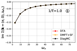
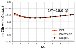
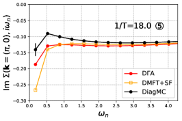
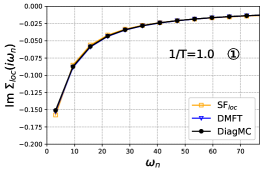
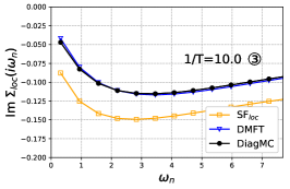
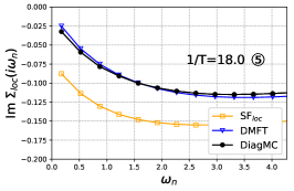
In the previous sections, we have seen that fluctuations from all momentum transfers contribute to the local (momentum-integrated) part of the self-energy in the metallic regime. Long-wavelength antiferromagnetic fluctuations associated with become increasingly important as temperature is lowered and are responsible for the formation of the pseudogap. This suggests to try a simple approximation in which one relies on DMFT for the local part of the self-energy, while a weak-coupling approximation Eq. (VII.1) is used to account for the non-local part, namely:
| (33) |
In this expression, the last term removes the local contribution from the spin-fluctuation formula, so that the local, -averaged part of the self-energy is entirely accounted for by DMFT. Please note that, in this subsection, we take the self-energy from paramagnetically restricted DMFT. To evaluate Eq. (33), we use the bare value of the coupling to spin fluctuations, and the DA spin susceptibility. We recall that the latter is simply given by: with the Moriya correction which ensures consistency with the Mermin-Wagner theorem and is determined such that , with being the local susceptibility as obtained in DMFT from the effective impurity model (for details see App. D.7). Expression (33) is actually a simplified version of the DA, in which vertex functions are set to unity (see also App. D.7 to recall of the DA equation of motion. For an analysis in the context of superconductivity in cuprates see Kitatani et al. (2019)).
The result of this simple ‘DMFT+SF’ approximation of Eq. (33) is compared in Fig. 24 (top row) to the DiagMC benchmark and to DA for three temperatures. We see that it performs excellently in the incoherent and in the metallic regime. In the pseudogap regime it is qualitatively reasonable, but overestimates the magnitude of the self-energy at low-frequency (in accordance with the observations made above.) This indicates that, for this rather weak value of the coupling , the vertex correction terms included in DA are not essential in the metallic regime, but become increasingly important as temperature is lowered into the pseudogap regime.
The lower panels in Fig. 24 display the local part of the self-energy as obtained from DMFT together with its approximation from weak-coupling spin fluctuation theory [the local term removed in Eq. (33)], in comparison to DiagMC. This clearly demonstrates that a weak-coupling spin fluctuation approximation does not provide a good estimate of the local component, even at this weak value of . In contrast, the non-perturbative DMFT provides an excellent description of the -averaged (local) self-energy, while non-local contributions can be reasonably accounted for by weak coupling spin fluctuation theory at this value of .
VIII Conclusion and outlook
In this article, we have purposefully focused on an apparently ‘simple’ regime of the two dimensional Hubbard model (simple square lattice, weak coupling, half filling) with three goals in mind: (i) assessing the ability of state-of-the-art computational methods to address the physics of this model at finite temperature, through the computation of a range of one-particle and two-particle observables (ii) providing an extensive assessment of basically all many-body methods currently available for this purpose, by comparing them to two very different Monte Carlo methods (DQMC and DiagMC) serving as benchmarks and, importantly (iii) investigating the rich physics associated with the different regimes and crossovers found in this model, as it evolves upon cooling from a high-temperature incoherent regime into a momentum-differentiated metal and eventually into an insulating regime with a pseudogap, and elucidating the nature and role of spin fluctuations in these different regimes.
It is satisfying to observe that the two benchmark methods considered in this article are successful at computing the properties of this model throughout the metallic regime and are in excellent agreement with each other. However, we also found that they face rather severe limitations when attempting to reach low temperatures, to the extent that only the onset of the pseudogap regime can be reached. Indeed, the pseudogap is associated with an exponentially growing antiferromagnetic correlation length which requires prohibitively large systems to be simulated with DQMC, while DiagMC, which in contrast works directly in the thermodynamic limit, is faced with convergence issues when summing the perturbative series at low-. We are hopeful that this can be overcome by using recent improvements of diagrammatic Monte Carlo based on the CDet algorithm Rossi (2017), together with improved schemes for summing the perturbative series.
Many of the methods considered in this article use the dynamical mean field theory (DMFT) as a starting point and treat spatial fluctuations beyond this starting point to various degrees of approximation. Obviously, the chosen regime of parameters puts DMFT very much out of its ’comfort zone’ since the physics at low- is dominated by long-range spatial fluctuations which in two dimensions also prevent long-range order at any non-zero temperature. Nonetheless we have emphasized and documented that, when properly interpreted, DMFT provides a useful initial description of the different regimes. Indeed, in the low- pseudogap regime when the correlation length is large, describing the system as long-range ordered is a reasonable mean-field starting point. Furthermore, remarkably, we found that DMFT provides a highly accurate determination of the local (momentum-averaged) self-energy, not only at high- as expected, but also through most of the metallic regime. This is a striking observation given that the correlation length reaches values as large as ten lattice spacing in this regime, and we further comment below on the physical reason explaining this finding.
Because of the very large correlation length at low-, cluster extensions of DMFT are not the best route to follow in this parameter regime of the Hubbard model. Although they succeed in describing the momentum-differentiated metallic regime in satisfactory agreement with the benchmarks, huge cluster sizes would be required to properly capture the pseudogap regime. Cluster extensions of DMFT are much better equipped for addressing strong coupling regimes with shorter correlation lengths.
In contrast, we found that extensions of DMFT (ladder-DA, TRILEX, ladder-DF and single-shot DB), that make use of response and vertex functions in order to take into account the contributions of fluctuations to the self-energy, perform much better here. We assessed their respective degree of accuracy and found that the DA and DF/DB methods are particularly successful at describing all physical regimes of interest in satisfactory agreement with the benchmarks, including the onset of the pseudogap regime. They also allow to enter deeper in the pseudogap regime: it is an open question for future work to assess their degree of validity in this low- regime when accurate and controlled benchmarks become available.
We have also considered many-body methods that do not make use of DMFT as a starting point, such as TPSC/TPSC+, fRG and the PA. TPSC played an important role early on in elucidating the physical origin of the weak-coupling pseudogap in relation to long-wavelength antiferromagnetic correlations. We found that it captures the different regimes qualitatively, but strongly overestimates the onset of the pseudogap temperature and the correlation length itself. TPSC+, a recent extension of the method, leads to significant improvements. In contrast, the PA underestimates the pseudogap onset temperature, especially at the nodal point, whereas it captures the behavior of double occupancy very accurately. The conventional one-loop fRG shown here is in qualitative agreement with the benchmark until its running coupling constants diverge. We remark, however, that the present implementation can be systematically improved by the recently introduced multiloop extension of fRG that converges to the parquet approximation Kugler and von Delft (2018b); Tagliavini et al. (2019); Kugler and von Delft (2018c), as well as expanding around the DMFT solution (DMF2RG) Taranto et al. (2014); Vilardi et al. (2019). Their combination, a multi-loop expansion of the fRG around DMFT, provides a very promising direction for future studies.
On the physics side, perhaps the most intriguing finding of our study is that, in the metallic regime, single-particle excitations with a lifetime that increases upon cooling appear to happily coexist with an antiferromagnetic correlation length which increases steeply, reaching about ten lattice spacings at the onset of the pseudogap. We have provided an explanation to this finding and also shown that spin fluctuations associated with the vicinity of the antiferromagnetic wave-vector are not the only important contributions to the self-energy in this regime. Fluctuations from all nesting vectors also contribute to the self-energy on the Fermi surface, and fluctuations from all momentum transfers contribute especially to the local, momentum-integrated, self-energy. This explains, importantly, why the latter is so accurately captured by single-site DMFT, even in the presence of strong antiferromagnetic fluctuations which are responsible for the momentum differentiation on the Fermi surface.
At the lowest temperatures, antiferromagnetic fluctuations eventually dominate, destroying the coherent metal which gives way to the pseudogap regime (with a narrow precursor regime at which the quasiparticle lifetime reaches a maximum). This provides a rationale for the success of methods such as DA and the DF, which incorporate fluctuations of all wave vectors beyond DMFT. In the parameter regime of interest, we have proposed and tested a simplified version of such an approach.
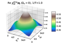
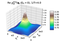


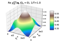
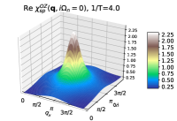
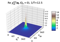
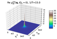
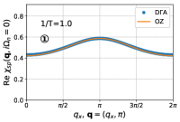
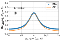
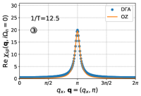
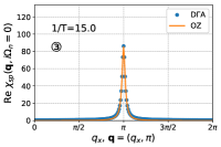
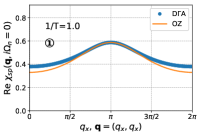
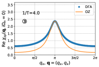
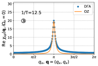
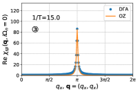
We have documented in details the rich sequence of crossovers occurring in this model upon reducing temperature, from an incoherent regime at high all the way down to the pseudogap regime at low-, through the intermediate temperature momentum-differentiated metal, and assessed the ability of the different computational methods to capture these crossovers. By analyzing the contribution of spin fluctuations, we showed that these different regimes are delimited by the comparison of temperature itself to the two characteristic energy scales and , or equivalently of the correlation length to the thermal de Broglie wavelength and to the length scale associated with Landau damping (with being the Landau damping constant).
Finally, we have also emphasized (Sec. VII.3.3 and Appendices B and C) the limitations of imaginary time/Matsubara computational methods in probing the delicate low energy non-Fermi liquid singularities of this perfectly nested model in the metallic regime.
Looking forward, the numerical, theoretical and physical insights obtained in this article should find direct applications in computational studies Kitatani et al. (2020); Galler et al. (2017); Kitatani et al. (2019) of materials for which the interplay between local electronic correlations and long-wavelength spin fluctuations play a crucial role, such as Sr2RuO4 Strand et al. (2019a); Tamai et al. (2019); Acharya et al. (2019) or the iron-based superconductors Zantout et al. (2019). On the model level, our findings will be immediately useful for describing how physical fluctuations (density, magnetic, pairing) on the two-particle level influence one-particle spectral functions and self-energies, and how quasiparticles are affected and sometimes destroyed altogether by these fluctuations Gunnarsson et al. (2016, 2017); Wu et al. (2017); Rohringer (2018); Arzhang et al. (2020); Gunnarsson et al. (2018); Schäfer and Toschi (2021).
Acknowledgements.
We would like to thank Andrey Chubukov, Chloé Gauvin-Ndiaye, Emanuel Gull, Karsten Held, Carsten Honerkamp, Andrey A. Katanin, Alexander I. Lichtenstein, Walter Metzner, Andrew J. Millis, Alice Moutenet, Georg Rohringer, Subir Sachdev, Michael Thoennessen, and Alessandro Toschi for useful and valuable discussions, as well as T. S. Barry for support and encouragement. T. S. and A. G. are indebted to Katharina Kölbl and Sandrine Kott for their infinite patience during the writing phase of this manuscript.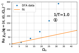
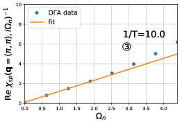
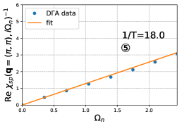
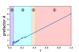
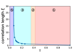
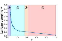
The present work was supported by: the Austrian Science Fund (FWF) through the Erwin-Schrödinger Fellowship J 4266 - “Superconductivity in the vicinity of Mott insulators” (SuMo, T.S.), and projects P 30997 (C.E.) and P 30819 (A. Kauch); the European Research Council for the European Union Seventh Framework Program (FP7/2007-2013) with ERC Grant No. 319286 (QMAC, T.S. and A.G.); the Simons Foundation through the Simons Collaboration on the Many Electron Problem (M.F., F.Š., E.K.); the Natural Sciences and Engineering Research Council (Canada) under grants RGPIN-2019-05312 (A.-M.S.T.) and RGPIN-2017-04253 (J.P.F.L.); the Canada First Research Excellence Fund, the Research Chair on the Theory of Quantum Materials, Compute Canada and Calcul Québec (Y.W., A.-M.S.T.). A. Kim and E.K. acknowledge funding from EPSRC through grant EP/P003052/1. V.H. and E.A.S. acknowledge the support by the North-German Supercomputing Alliance (HLRN) under the Project No. hhp00042. C.H. and S.A. acknowledge financial support from the Deutsche Forschungsgemeinschaft (DFG) through Projects No. AN 815/4-1 and No. AN 815/6-1. T.S., F.Š. and M.F. acknowledge the hospitality of the Center for Computational Quantum Physics at the Flatiron Institute. The Flatiron Institute is a division of the Simons Foundation. The authors acknowledge the computer support teams at CPHT École Polytechnique, CEA Saclay (IPHT-LSCE) and at the Flatiron Institute as well as the computer service facility of the MPI-FKF for their help. This work was granted access to the HPC resources of TGCC and IDRIS under the allocations A0070510609 and A0090510609 attributed by GENCI (Grand Equipement National de Calcul Intensif). Parts of the simulations were performed on computers provided by Calcul Québec, and Compute Canada. J.P.F.L. acknowledges computational support from ACENET and Compute Canada. The PA calculations have been done on Vienna Scientific Cluster (VSC) and JURECA at Forschungszentrum Jülich Jülich Supercomputing Centre (2018). D. R. gratefully acknowledges the computing time granted through JARA on the supercomputer JURECA Jülich Supercomputing Centre (2018) at Forschungszentrum Jülich.
Appendices
Appendix A Ornstein-Zernike form of the magnetic susceptibility
Close to a magnetic phase transition, the magnetic susceptibility (bosonic propagator) assumes the following Ornstein-Zernike form Ornstein and Zernike (1916):
| (34) |
with being a prefactor, the Landau damping constant (the dynamical critical exponent has been set to here), and the magnetic correlation length. This form can be used to evaluate the spin-fluctuation diagram given in Eq. (VII.1). In the renormalized classical regime ⑤, the sum may be restricted to the lowest Matsubara frequency without great loss of precision, which is, however, not possible in the metallic regime ③. The estimation of the correlation length from the static magnetic susceptibility in this manuscript has been performed by an empirically more robust formula (especially in the limit of small ) of the Ornstein-Zernike form, which incorporates the lattice (tight-binding) structure of the problem Rohringer et al. (2011), neglecting a possible anomalous exponent (cf. for the three-dimensional Heisenberg model Huang (1987)):
| (35) |
and reduces to the original form in the long wavelength limit (small arguments of the sine). For the fits shown we fixed . Fig. 25 shows data for the static antiferromagnetic susceptibility in DA (upper row) and the respective Ornstein-Zernike fits for various temperatures. Please note again, as discussed in the main text, that the Ornstein-Zernike fit is most accurate only around the vicinity of and may not capture the physics at other points, important e.g. in the metallic regime (see Sec. VII.3). These fits of the static antiferromagnetic susceptibility are used to determine the prefactor and the magnetic correlation length . For extracting the Landau damping , and have been fixed and has been fitted from the frequency dependence of the propagator. The upper panels of Fig. 26 show these fits of DA data for three representative temperatures. The lower panels show the obtained parameters , and as a function of temperature.
We see that the prefactor rapidly decreases with temperature in the metallic regime. This can be rationalized by observing that the local susceptibility obeys a Curie-Weiss law in this regime, implying that and hence that decreases linearly with . In contrast, in the low- insulating regime, the sum-rule implies and hence reaches a constant value at low . For the temperature dependence of the local spin susceptibility in DA see Fig. 27. The (negative) imaginary part of the local self-energy extrapolated to zero Matsubara frequency as a function of temperature, relevant for the discussion in Sec. VII.3.2, is shown in Fig. 28.
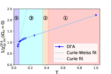
Appendix B Low-frequency expansion of the self-energy
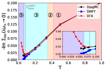
In a Fermi liquid, the self-energy on the Fermi surface can be expanded at low (imaginary) frequency as a Taylor series:
| (36) | |||||
Inserting this expression into Dyson’s equation , we see that the spectral function displays a quasiparticle peak with a spectral weight and width (inverse of the quasiparticle lifetime ) given by:
| (37) | |||||
| (38) |
Performing also a Taylor expansion for momenta close to Fermi surface, the renormalization of the quasiparticle effective mass is obtained as:
| (39) |
In practice, and , as displayed e.g. in our discussion of the metallic regime in Fig. 19, are obtained in this article by a fit of the imaginary part of the self-energy calculated on the discrete set of Matsubara frequencies, by a fourth-order polynomial. This is common practice in analyzing computational results available in imaginary time at finite temperature. The sign of the slope of the self-energy at low Matsubara frequencies was also used to distinguish between ‘metallic’ behaviour () and the pseudogap and incoherent regimes in which the positive slope corresponds formally to . Care should be applied, however, in interpreting the values of and obtained from such Matsubara fits in terms of quasiparticles properties, when the system does not obey Fermi liquid behaviour at low frequencies or low temperatures (as is the case here, because of perfect nesting and of the gradual opening of the pseudogap). We illustrate and clarify this point by considering, for simplicity, a linear fit of the imaginary part of the self-energy over the first two Matsubara frequencies , , namely:
| (40) |
with:
| (41) |
For simplicity, we have dropped the momentum dependence in these expressions: it is understood that the analysis is performed at a given value of . We now use the spectral representation of the self-energy with , yielding:
| (42) |
Substituting this into Eqs. (B), after simple algebra, we finally obtain:
We now analyze how these two quantities behave in the low-temperature limit. To this aim, we consider cases in which scaling applies for small and (but an arbitrary ratio ), and that with a scaling function such that and . The case corresponds to a Fermi liquid for which the scaling function is known to be . A value of corresponds to non-Fermi liquid behaviour with scaling, as found for example close to quantum critical points controlled by strong coupling fixed points Sachdev (1999). For an analysis of non-Fermi liquid behaviour and scaling within second order perturbation theory, see Appendix C.
To obtain the low- behaviour of , we observe that the scaling form can be directly substituted in the above expression while preserving the convergence of the integral. This leads to, for :
| (43) |
This expression demonstrates that a fit to the self-energy on Matsubara frequencies is able to correctly capture the non-Fermi liquid temperature dependence of the scattering rate. Note that for this to hold, it is crucial that scaling indeed applies. This derivation has been performed for simplicity for a linear fit, but extends to a higher order polynomial fit.
The low- analysis of proceeds along slightly different lines. Indeed, direct substitution of the scaling form into the equation above would lead to an ultraviolet divergent integral when . In that case, the limit can directly be taken to yield:
| (44) |
This is indeed the exact expression of the quasiparticle weight resulting from the spectral representation. Note that, for with at low frequency, the above integral converges in the infrared, and that in that case there are coherent quasiparticles, with a finite spectral weight and a scattering rate smaller than their energy. In the opposite case , the scaling function must be used which yields the low- behaviour:
At low-, vanishes at indicating the breakdown of the quasiparticle concept. For a very slow logarithmic vanishing of is expected.
In conclusion, this analysis demonstrates that when scaling applies together with a simple power-law behaviour, a fit to the self-energy over Matsubara frequencies is able to pickup the correct -dependence of the scattering rate and quasiparticle weight in both the Fermi liquid and non-Fermi liquid case, in spite of the fact that the frequency dependence of the self-energy for is inaccessible from Matsubara frequencies. scaling typically applies in the quantum critical regime associated with quantum critical points (QCP) controlled by a strong coupling fixed point Sachdev (1999). In this work, the QCP is the one associated with the disappearance of antiferromagnetism at , and hence it is not clear whether scaling applies in the metallic regime. Logarithmic violations may be expected, for example.
Appendix C Self-energy from second order perturbation theory
For further reference, and to facilitate the discussion of the consequences of perfect nesting in Sec. VII.3.3, here we show the results of second order perturbation theory (2PT) for the self-energy.
C.1 Real frequencies
We first consider the self-energy in 2PT on the real frequency axis (see also Lemay (2000); Rohe and Honerkamp (2020)). Its functional form can be gained by careful analytic calculations performed in Sec. 4.4 of the PhD thesis of F. Lemay Lemay (2000) that we summarize in this subsection. We start by considering the expression on the Matsubara axis
| (45) |
with the (non-interacting) bubble
| (46) |
and being the non-interacting Green function.
C.1.1 Analytical considerations
Analytic continuation of Eq. (45) gives
where denote Fermi- and Bose distribution functions, respectively, is the principal value and . These expression show that at frequencies lower than the temperature (and, therefore, smaller than the first Matsubara frequency), the self-energy takes a clear non-Fermi-liquid form for Fermi-surface vectors (see also Sec. VII.3):
| (49) |
and
| (50) |
with .
The singular behavior of the self-energy at low frequency comes from the singular behavior of the imaginary part of the susceptibility
| (51) |
where and
| (52) |
The origin of these singularities, that appear at small frequency when is near the diagonal, can be understood roughly from the fact that for any external momentum located near the diagonal of the Brillouin zone, there are electrons near the half-filled diamond Fermi surface that can be scattered to electrons also near the Fermi surface.
More precisely, suppose that an electron below the Fermi surface at is excited above the Fermi surface at such that . All internal momenta in the bubble must be considered, while and are fixed. But the velocity of the particle-hole excitation vanishes at for any value of That leads to van Hove-like singularities in the particle-hole excitations. The integral over gives logarithmic contributions to that are finite, except for where they diverge when is different from zero. Note that the singular frequency vanishes when is on the diagonal.
These singularities influence the low frequency behavior of the imaginary part of the self-energy as follows. We are considering now the imaginary part in Eq. (C.1.1) and integrate over the -distribution to arrive at
| (53) | |||||
For the sake of detecting non-Fermi liquid behavior, we are interested in the regime where the inequality is satisfied. In that regime, it is the classical limit of the Bose function that dominates and singularities come only from integrals of the logarithms in Eq. (51), whose arguments then are
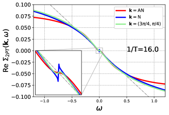
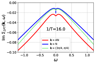
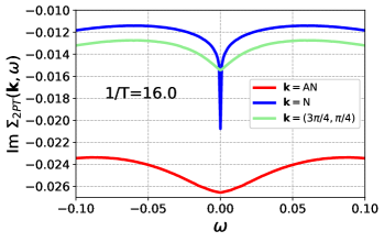
We take the integral over to run over the Brillouin zone, then the integral over is restricted by the Bose function to a range near the diagonals where the inequality is satisfied. This determines the limits of integration over to be of order away from the diagonal. The argument of the logarithm , when expanded near the diagonal, can be approximated by
| (54) |
The integral over can be done, leading to other logarithms that depend on . The singular part of the remaining integral comes from regions where is small. The final result is obtained by expanding around values of where vanishes. In the Taylor expansion of there are terms linear in that give the final result for everywhere, except when the linear term in the expansion of vanishes, which occurs for There, the leading term scales as which modifies the integral over and leads to proportional to The Fermi points seem special because it is there that the energy associated with particle-hole excitations can be small for the largest range of values of near the diagonal.
C.1.2 Numerical evaluation
In Fig. 29 we show the numerical evaluation of these expressions for the real (first panel) and imaginary part (second and third panel) for and , i.e. deep inside the metallic regime for the antinode (red), node (blue) and generic point (light-green). In both real and imaginary parts one can clearly see non-Fermi liquid behavior at low frequencies: at low frequencies, the slope of the real part is reversed for the node and the generic -point and non-linear also for the antinode. For comparison we also show (with the dotted-dashed line) the respective low frequency result from Fermi-liquid fit from the Matsubara axis (see later in this Appendix), which are oblivious of the features at .
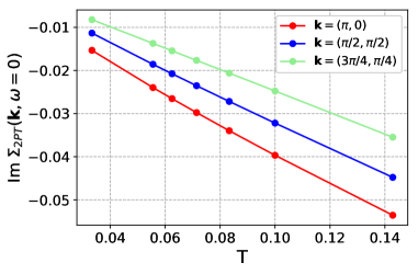
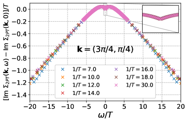
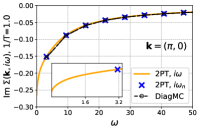
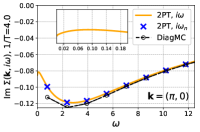
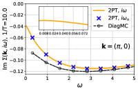
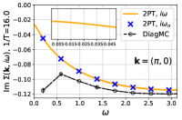
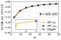
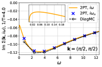
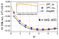
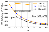
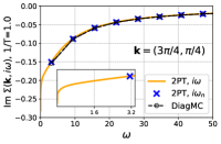
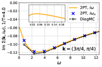
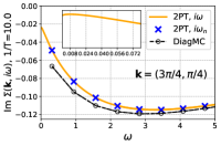
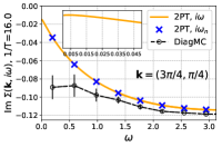
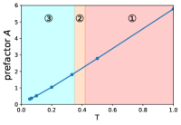
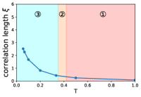
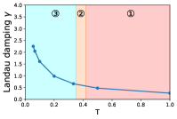
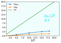
Focusing on the imaginary part, one can observe that, despite their different magnitudes, the functional forms of the antinode and the generic point are very similar. The node, however, exhibits a completely different functional behavior, eventually resulting in for very small frequencies, and indeed compatible with a square root behavior. Additionally to its frequency behavior we extracted the zero-frequency dependence on temperature, shown in the upper panel of Fig. 30. Although -corrections are expected Lemay (2000), the dependence appears rather linear. Eventually, with our precise numerical data, we can numerically demonstrate that indeed exhibits scaling as discussed in the main text, by plotting over (lower panel of Fig. 30), which results in an excellent data collapse over a broad temperature (and frequency) range inside the metallic regime. However, as already stated in App. B, scaling typically applies in the quantum critical regime associated with quantum critical points (QCP) controlled by a strong coupling fixed point Sachdev (1999). The QCP present is associated with the disappearance of antiferromagnetism at , and hence it is not clear whether scaling generally applies (e.g. logarithmic corrections may be expected).
C.2 Imaginary frequencies and comparison
In order to compare our findings on the real axis with the DiagMC benchmark, we directly evaluate Eq. (45) on the Matsubara axis. We used meshes of Matsubara frequencies and a linear momentum mesh of for the summations performed. Fig. 31 shows the 2PT data (blue crosses) in comparison to the DiagMC benchmark (black circles and dashed line) for the antinode (uppermost row) and node (second row) as well as for the generic point [third row] for various temperatures. The benchmark result is described quantitatively by 2PT in the incoherent regime and fairly well inside the high temperature metallic regime. In particular, 2PT exhibits a clear momentum differentiation between node and antinode. However it fails in the description of the pseudogap, i.e. the regimes ④ and ⑤ are absent. This is particularly apparent comparing the emerging energy and length scales obtained from Ornstein-Zernike fits (last row, cf. discussion in Sec. VII.3 and Fig. 20).
However, as already discussed before, this may be quite hard to judge by looking at data from the Matsubara axis only. Therefore, we additionally computed the self-energy in 2PT on a continuous imaginary frequency grid (solid orange lines in Fig. 31, see insets for a zoom 111For obtaining the data on the continuous imaginary frequency axis, in a first step, has been calculated on the real axis. After retrieving via the Kramers-Kronig relations, the Cauchy formula has been used for the forward continuation onto the imaginary axis. The calculation on the real axis profits from analytical treatments of the delta function which reduces the quadrature dimensions.). One indeed observes that, for frequencies way smaller than the ones accessible by a Matsubara grid , the slope of the imaginary part of the self-energy changes, at least in this fully nested case, to being positive, yielding clear non-Fermi liquid behavior. This behavior is particularly emphasized at the nodal point (second row).
Using a Fermi-liquid ansatz (see App. B), one can extract a momentum-dependent quasiparticle weight and inverse quasiparticle lifetime from the Matsubara axis (Fig. 32). As already discussed in the main text, these parameters are only meaningful (in the strict sense of describing Landau quasiparticles) if the low-frequency behavior of the self-energy is the ”correct” one, i.e. compatible with the one expected by a Fermi liquid (e.g. in exhibiting a negative slope and a long quasiparticle lifetime). In order to estimate the quality of this plain Matsubara fit, we show the ”offset” from both the real frequency data (crosses in the lowest panel of Fig. 32) and the Matsubara fits. We notice that both methods of extraction are in a very good agreement inside the metallic regime, except at the nodal point, where a severe underestimation by the Matsubara data of is found.
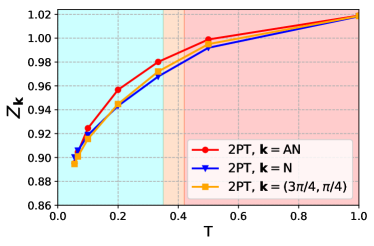
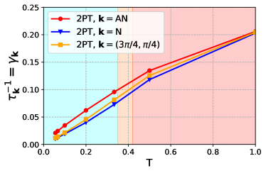
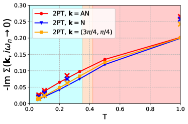
Appendix D Brief description and references of the presented methods
As one of the goals of this manuscript is a synopsis of a variety of different modern many-body techniques, in this Appendix, we will give a short overview on these. Of course, the Appendix cannot serve as an exhaustive review, but will contain the basic idea of each method as well as the necessary references for further information and, if necessary, computational details for obtaining the results presented in this paper.
D.1 DiagMC
Diagrammatic Monte Carlo (DiagMC), first developed by B. Svistunov and N. Prokofiev Prokof’ev and Svistunov (1998), is based on the idea of stochastically sampling Feynman diagrams contributing to a perturbative expansion directly in the thermodynamic limit. In a broad sense, the Diagrammatic Monte Carlo approach consists of the choice of a diagrammatic expansion for a given observable, a numerical algorithm computing the corresponding expansion coefficients and, if necessary, the resummation techniques applied to the resulting perturbative series.
The physically most natural Abrikosov et al. (1975), skeleton, expansions are potentially dangerous when applied to the two-dimensional fermionic Hubbard model as they can converge to wrong results in the vicinity of half-filling or whenever the local magnetic moment develops Kozik et al. (2015); Rossi and Werner (2015); Gunnarsson et al. (2017); Kim and Sacksteder (2020); Chalupa et al. (2021). In contrast, bare expansions have a well-defined analytic structure and generally have a non-zero convergence radius in the two-dimensional fermionic Hubbard model. Such expansions can be constructed around an arbitrary starting point Wu et al. (2017); Rossi et al. (2016); Chen and Haule (2019); Rossi et al. (2020); Šimkovic et al. (2020). The default choice Van Houcke et al. (2010); Kozik et al. (2010) is to expand around the non-interacting Hamiltonian with the chemical potential shifted by a constant ( at half-filling) Rubtsov et al. (2005), which effectively eliminates all diagrams with Hartree-type insertions, leading to a much improved variance, which is what we adopt here.
The choice of algorithm used to compute the expansion coefficients determines how large expansion orders can be obtained with reasonable error bars. In this publication we employ the currently most efficient class of algorithms, based on the Connected Determinants Diagrammatic Monte Carlo (CDet) introduced for connected quantities by R. Rossi Rossi (2017) and generalized to the evaluation of one-particle irreducible self-energy diagrams in Refs. Šimkovic et al. (2020); Moutenet et al. (2018); Rossi (2018). The particular self-energy implementation used in this publication is DDMC from Ref. Šimkovic and Kozik (2019) as it is very well-suited for the computation of specific -points directly in momentum-space. In its original formulation, CDet only works with bare diagrammatic expansions (consisting exclusively of interaction vertices and bare propagators ), although a generalization to semi-bold Rossi et al. (2016) and bold Van Houcke et al. (2012); Deng et al. (2015) schemes has recently been developed Rossi et al. (2020); Šimkovic et al. (2020). Contrary to previously developed Diagrammatic Monte Carlo algorithms Prokof’ev and Svistunov (2008, 2007); Van Houcke et al. (2010); Kozik et al. (2010); Van Houcke et al. (2012); Deng et al. (2015); Šimkovic IV. et al. (2019) which evaluate a single Feynman diagram at each Monte Carlo step, CDet computes a factorial number of relevant diagrams permuted over all internal vertices at exponential cost, scaling with the expansion order as for connected quantities Rossi (2017) and for one-particle irreducible quantities Šimkovic et al. (2020); Moutenet et al. (2018); Rossi (2018) (or, alternatively, scaling as and , respectively Björklund et al. (2007)). This is achieved by grouping all possible diagram topologies of a particular diagram order into determinants and subsequently subtracting all disconnected, and in the case of the self-energy also all one-particle-reducible, diagrams from the sum by using a recursive formula. As a consequence of the exponential scaling, the total error of a convergent series scales polynomially with computational time Rossi et al. (2017). The statistical variance of the algorithm only allows for the computation of a finite number of expansion coefficients, typically (compared to for previous Diagrammatic Monte Carlo algorithms).
In challenging cases, such as low temperatures and/or high values of physical coupling, resummation techniques are needed to evaluate the series close to, or beyond the, radius of convergence. This constitutes the only source of systematic error in this approach. A protocol for the resummation of extrapolation, which gives control over this systematic error, has been developed in Ref. Šimkovic and Kozik (2019).
At half-filling, every other order is equal to zero for the double occupancy (even) as well as for the self-energy evaluated at every -point on the non-interacting Fermi-surface (odd). A consequence of particle-hole symmetry at half-filling is that a single calculation of the expansion coefficients at a given temperature yields results for all values of , provided the series is resummable (away from half-filling this is still the case, however the evaluated density also changes as a function of interaction strength ). For all presented observables, the limiting factor to the applicability of this approach at high enough interactions and low enough temperatures is the presence of singularities in the vicinity of the positive real axis in the complex plane of interaction strength , which render the resummation of the series prohibitively hard. Despite the fact that, in this publication, series have only been evaluated within their radius of convergence, resummation by means of Padé and Dlog-Padé approximants Šimkovic and Kozik (2019); Brezinski (1996); Gonnet et al. (2013) has been performed in order to accelerate the convergence of series whilst controlling the systematic error of the extrapolations. In the half-filled two-dimensional Hubbard model, this approach has previously allowed for numerically exact results that shed light on the metallic to quasi-antiferromagnet crossover as described by the self-energy Šimkovic et al. (2020) as well as various other thermodynamic observables Kim et al. (2020); Lenihan et al. (2021).
D.2 DQMC
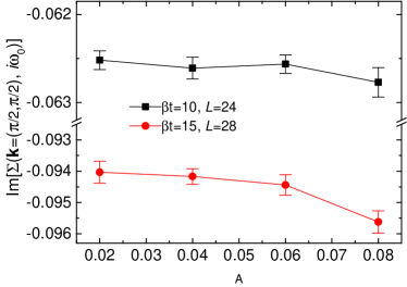
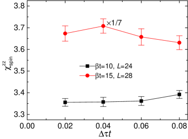
The determinantal Quantum Monte Carlo (DQMC) algorithm, formulated by Blankenbecler, Scalapino, and Sugar Blankenbecler et al. (1981), is a controlled method and has been widely applied to finite-temperature simulations of correlated fermion systems. Its basic methodology is to transform two-body interactions into free fermions coupled with auxiliary fields and then sample the fields to compute fermionic observables. To achieve this, a Trotter decomposition (such as is used in this work, where and are the tight-binding and interacting parts of the model Hamiltonian), and a Hubbard-Stratonovich (HS) transformation (the discrete spin decomposition Hirsch (1983) for on-site Hubbard interaction is used in this work) are applied within the discretization for the inverse temperature as . When convergence can be established, the method is numerically exact.
The systematic error from finite is controllable and can be eliminated by extrapolating simulations with several different values. In Fig. 33, we present representative results of systematic Trotter errors in DQMC simulations. Two systems, with and with , are studied. We concentrate on the self-energy at (upper panel) and the spin susceptibility (lower panel). The results for both parameters explicitly show the convergences to the limit for within our statistical uncertainty. This means that our choice of is reliable.
Further details about DQMC algorithm can be found in several review papers Assaad and Evertz (2008); Chang et al. (2015). We have also implemented our most recent improvements He et al. (2019a, b) of this method in this work. The minus sign problem is absent for the Hubbard model at half filling studied in this work and DQMC method can reach large system sizes. For the calculation of dynamical quantities, the imaginary-time single-particle Green function and correlation functions are measured in DQMC simulation, and then the imaginary-frequency observables are obtained through the Fourier transformation. The Dyson equation was then applied to compute the self-energy. For the case, convergence to thermodynamic limit of all the physical observables is observed for up to for . For lower temperatures, we perform finite-size scalings using second-order polynomials with constraints of monotonic behaviors to reach the thermodynamic limit. We typically use between to measurement samples for systems with linear system size from to . In DQMC the number of Matsubara frequencies is determined by the number of imaginary time slices , which in turn depends on the Trotter step, chosen here to be as mentioned earlier.
D.3 MFT
The calculation of the static mean-field theory (MFT) susceptibility is analytically equivalent to the (non-selfconsistent) random phase approximation (RPA). The idea of the RPA, originally introduced in Bohm and Pines (1951), is building ladders for the susceptibilities with the bare interaction in the physically relevant channel, utilizing the non-interacting susceptibility Eq. (46). The fermionic propagator, thus, is the non-interacting Green function . The interacting susceptibility is obtained via:
| (55) |
We used momentum grid with a maximum linear mesh sizes of and and the number of fermionic Matsubara frequencies being .
D.4 DMFT
The dynamical mean field theory (DMFT) has become one of the standard techniques for tackling strongly correlated systems over the past decades. Its basic idea consists in mapping the full lattice Hamiltonian Eq. (1) onto a self-consistently determined single site Anderson impurity model. This procedure is exact in infinite dimensions, but represents an approximation in finite dimensions due to its neglection of spatial correlations. Hence, the self-energy in DMFT is purely local. For further reading about the details of the algorithm we recommend the seminal papers Georges and Kotliar (1992); Metzner and Vollhardt (1989) and the review Georges et al. (1996). The self-energy and magnetization data presented in this paper have been produced using a state of the art continuous time quantum Monte Carlo impurity solver in its interaction expansion (CT-INT Rubtsov and Lichtenstein (2004); Rubtsov et al. (2005); Gull et al. (2011a)), which is, like the DMFT self-consistency scheme, entirely implemented in the TRIQS framework Parcollet et al. (2015). For the calculation of the (magnetic) susceptibility and correlation length we used data from both (i) an exact diagonalization (with four bath sites) impurity solver and the implementation of the Bethe-Salpeter equations presented in Rohringer et al. (2018b) and (ii) the CT-INT solver and tprf framework of TRIQS Strand et al. (2019b), carefully crosschecking that they obtain the same results. As the magnetic correlations (and correlation lengths) grow exponentially reaching low temperatures, we used a very dense momentum grid for these data with a maximum linear mesh sizes of and and the number of fermionic Matsubara frequencies being . In the case of the CT-INT impurity solver, we used Monte Carlo steps.
Cluster extensions of DMFT: DCA, CDMFT
D.5 DCA
The dynamical cluster approximation (DCA) Hettler et al. (1998, 2000); Maier et al. (2005a) is an embedding technique wherein the electron self-energy is obtained from the solution of an impurity model with interacting sites coupled to an infinite bath. As such, the DCA is just one particular generalization to of the ‘single site’ dynamical mean field method that becomes exact as the number of impurity sites Georges and Kotliar (1992); Georges et al. (1996); Maier et al. (2005a). The DCA formulation partitions the Brillouin zone into equal area tiles and approximates the self-energy in each tile , as a piecewise constant function of momentum as
| (56) |
where if and for . Similar to DMFT, DCA invokes a self consistency loop where an initial guess for the impurity model parameters produces a set of which are then used to update the bath. In this work we obtain results for large values of in the paramagnetic phase but note that at weak-coupling and low temperatures studied in this work the DCA expansion in cluster size does not appear to be in a scaling regime and therefore one needs much larger clusters in order to estimate the infinite system size limit Šimkovic et al. (2020); LeBlanc and Gull (2013).
To solve the site impurity problem we use the continuous time auxiliary field method Gull et al. (2008b, 2011a) with submatrix updates Gull et al. (2011b). Similar to other methods that employ Hubbard-Stratonovich decoupling, the primary computational hurdle is finding determinants of an matrix where is referred to as the expansion order. Unlike Hirsch-Fye solvers that employ a fixed the expansion order and time steps in CT-AUX are not fixed, an important improvement that removes the necessity for a extrapolation. In the case of DCA, applying CT-AUX to clusters of size results in an expansion order Gull et al. (2008a). In this work we have presented data primarily for fixed cluster size on a bipartite cluster. The DCA self-consistency is presumed to be paramagnetic and is iterated times until the deviation between iterations is much less than the statistical error obtained from samples of each frequency up to . Our DCA and CT-AUX codes are based on the ALPS libraries Gaenko et al. (2017); Wallerberger et al. (2018).
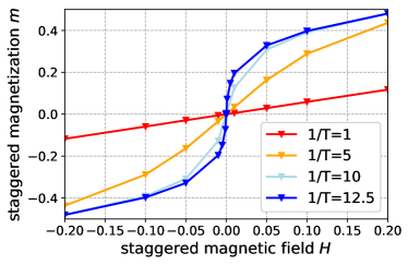
D.6 CDMFT
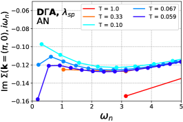
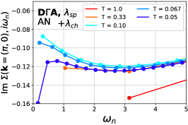
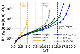
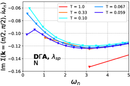
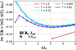
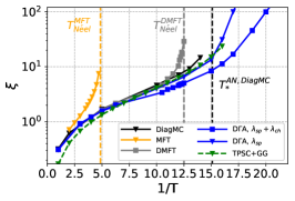
Cellular dynamical mean-field theory (CDMFT) is the real space cluster extension of DMFT Maier et al. (2005a); Parcollet et al. (2004); Sakai et al. (2012); Park et al. (2008). While proposed around the same time, it has up to today been less spread than the complementary dynamical cluster approximation which is formulated in momentum space. The impurity of the auxiliary Anderson model in CDMFT consists usually, contrary to single site DMFT, of superstructures obtained by upfolding the lattices unit-cell. On the square lattice, e.g., these may consist of quadratic patches. Hence, non-local correlations are included on length scales given by the cluster size as intersite single-particle self energies. Even within the aforementioned patch geometries, which typically retain point group symmetry, translational symmetry is broken (for even within the cluster). Re-periodization schemes suffer from ambiguity and may even lead to convergence problems when attempted inside the self-consistency loop. The lattice quantities are therefore approximated from the converged CDMFT solution by restoring the translational invariance for the Green function, the self-energy, or its cumulants Lichtenstein and Katsnelson (2000); Kotliar et al. (2001); Stanescu and Kotliar (2006); Sakai et al. (2012, 2009); Staar et al. (2013); Sakai et al. (2016); Verret et al. (2019). This study uses a cumulant scheme presented in App. B of Klett et al. (2020).
A recent study Klett et al. (2020) has shown that a so-called center-focused extrapolation of self energies (and even susceptibilities) to infinite cluster sizes (with a linear regression in ) yields the best results in comparison to numerically exact diagrammatic quantum Monte Carlo calculations. The CDMFT+CFE self-energies presented in this paper have been obtained by considering quadratic patches of up to for the extrapolation scheme. The auxiliary impurity models were solved using a state-of-the-art continuous time quantum Monte Carlo impurity solver in its interaction expansion (CT-INT Rubtsov and Lichtenstein (2004); Rubtsov et al. (2005); Gull et al. (2011a)) implemented in the TRIQS framework Parcollet et al. (2015). We used 20 CDMFT self-consistency loops (until convergence). Afterwards we performed 30 simulations with different random seeds starting from this previously converged solution. We take the self-energy as the mean of these 30 simulations. The solver parameters were a cycle length of 300, 10000 warmup cycles and cycles.
For the calculation of the magnetic susceptibility we applied an antiferromagnetic staggered field and measured the staggered magnetization . We then linearized the curve at small fields:
| (57) |
Fig. 34 shows a sample of these curves for various temperatures. The transition to an antiferromagnetic ordered state is signalled as a vertical tangent at , i.e. as divergence of the susceptibility, at . This represents a very small correction w.r.t. DMFT, where .
Diagrammatic extensions of DMFT
A different route for the inclusion of spatial correlations on top of DMFT is taken by its diagrammatic extensions. Their principle is to extract a higher order correlation function from an auxiliary impurity model and consistently calculate the desired observables from it. For a very recent overview of diagrammatic extension of DMFT see Rohringer et al. (2018a). More detailed information for each method is given below.
D.7 DA
In the dynamical vertex approximation (DA) Toschi et al. (2007); Katanin et al. (2009) the two-particle analog of the self-energy, the fully irreducible two-fermion scattering vertex , in a DMFT spirit, is assumed to be purely local. In order to obtain the corresponding susceptibilities and self-energies, without the knowledge of leading instabilities, the parquet equations have to be solved self-consistently (see Valli et al. (2010, 2015) for nanoscopics, Kauch et al. (2020) for -tons and Eckhardt et al. (2020); Kauch et al. (2019) for the two-dimensional Hubbard model). However, if (like in the present case of the Hubbard model), the leading instability is known, the scheme can be significantly facilitated by considering only the Bethe-Salpeter in the associated scattering channel and the Dyson-Schwinger equation, in order to obtain susceptibilities and self-energies (for successful applications see Rohringer et al. (2011); Valli et al. (2015); Schäfer et al. (2015b); Galler et al. (2017); Schäfer et al. (2015a, 2016a); Pudleiner et al. (2016); Schäfer et al. (2017, 2019); Del Re et al. (2019); Kitatani et al. (2020); Klebel-Knobloch et al. (2021)). In the vicinity of a phase transition, in order to restore the proper sum rules for the susceptibilities (and, thus, the asymptotics of the self-energy and therefore the two-particle self-consistency), within the ladder-version of the DA, a Moriyaesque so-called correction is used Toschi et al. (2007); Katanin et al. (2009); Schäfer (2016); Rohringer and Toschi (2016). For the results presented in the main text of the current manuscript, this correction is only done for the spin susceptibility (, see below). For the calculation of the (magnetic) susceptibility and correlation length we used data from an exact diagonalization (with four bath sites) impurity solver and the implementation of the Bethe-Salpeter equations and Dyson-Schwinger equation presented in Rohringer et al. (2018b) (again, like in the DMFT case) were crosschecked with CT-INT. We used momentum grid with a maximum linear mesh sizes of and and the total number of fermionic as well as bosonic Matsubara frequencies being . In the perspective of a future improved version of a Moriyaesque -correction Katanin et al. (2009); Rohringer and Toschi (2016), it is instructive to also compare the results obtained with the correction in both particle-hole channels (i.e. charge and spin, , see Eq. (6) in Rohringer and Toschi (2016))
| (58) |
(with ) to the ones obtained only with a correction in the spin channel (, Eq (5) in Rohringer and Toschi (2016)):
| (59) |
Results for both schemes are presented in Fig. 35. In comparison with DiagMC in Fig. 10, the self-energy obtained with would lead to a slightly better agreement of the imaginary part at low frequencies at the antinode in comparison to the benchmark (left and central panel), but a slightly worse agreement for the susceptibility, the correlation length and (right panel). It should be noted that the spin susceptibility and correlation length of DA with agrees almost perfectly with a version of TPSC+ coined TPSC+GG down to low . A more detailed comparison of different TPSC variants is done in App. D.11. Eventually, in order to be able to compare the simple DAesque approximation discussed in Sec. VII.4, we recall the Dyson-Schwinger equation of motion for the ladder-version of the DA (see Toschi et al. (2007); Katanin et al. (2009); Rohringer (2013), here omitting the Hartree term):
where refers to the physical, Moriya-corrected susceptibility, denotes the full two-particle vertex from the self-consistently determined Anderson impurity model in DMFT and and the last line of the equation accounts for double counting corrections of the local part of the self-energy. denotes the electron-boson coupling vertex (already integrated over the internal momentum ). For the simple approximation in Sec. VII.4, the electron-boson coupling vertex is set to unity for all momenta and frequencies. A precise definition of the components of the equation of motion can be found at Eq. (4.19) of Rohringer (2013).
D.8 TRILEX
The triply irreducible local expansion (TRILEX) method is a relatively recent approach to strong correlations, which utilizes the decoupling of the fermion-fermion interaction of the Hubbard Hamiltonian into auxiliary bosons Ayral and Parcollet (2015, 2016). For these bosons, the fermion-boson vertex of a self-consistently determined impurity model is extracted and the lattice polarization and self-energy are calculated via Hedin’s equations. The beauty of this approach consists in the facts that (i) the fermion-boson vertex is relatively easy to calculate (compared to the four-point vertex) and (ii) the convergence of the method to the exact solution can be achieved via a cluster extension of TRILEX Ayral et al. (2017) (we used DCA clusters with two and four sites in this paper) and (iii) the extension for treating superconductivity is straight forward Vučičević et al. (2017). However, the interaction is not unique and comes at the price of introducing an additional (Fierz) parameter , which in this paper was set in such a way that we decouple only the spin channel (i.e. in Heisenberg spin decoupling Ayral and Parcollet (2016)). This choice can be motivated by a so-called fluctuation diagnostics analysis of the self-energy in the pseudogap regime of the Hubbard model Gunnarsson et al. (2015). A different route to enhance the results of TRILEX can be made by inserting the fermion-boson vertex on both sites of the Hedin equations (an approach which we called TRILEX , see also Stepanov et al. (2016a, 2019a) for a similar idea in the dual theories, see also Krien (2019) for an efficient evaluation of the polarization bubble in DMFT and Krien et al. (2017) for the question of conservation in two-particle self-consistent theories). The self-energies in the main text using this method show results which turn out to be similar to cluster TRILEX. We used momentum grids with a maximum linear mesh sizes of and and the number of fermionic and bosonic Matsubara frequencies were chosen as and , respectively. For the impurity solver (CT-INT Rubtsov and Lichtenstein (2004); Rubtsov et al. (2005); Gull et al. (2011a)) we used Monte Carlo steps.
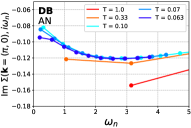
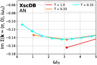
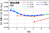
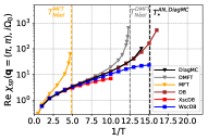
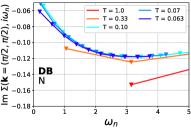
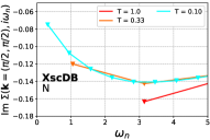
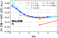
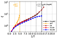
D.9 DF
The dual fermion approach Rubtsov et al. (2008, 2009); Hafermann et al. (2009) is a diagrammatic extension of the single site dynamical mean field theory (DMFT), motivated by the idea that non-local corrections to DMFT can be captured by a perturbative expansion around a solution of the dynamical mean field impurity problem.
In the dual-fermion formalism Rubtsov et al. (2008); Antipov et al. (2015) one replaces the lattice problem with a lattice of coupled Anderson impurity problems resulting in an action of the form
| (61) |
with , and where is the momentum independent Green function of the Anderson impurity problem, and is the hybridization function between the impurity and the bath Georges et al. (1996); Rubtsov et al. (2008). The dual-fermion action now depends on and which are dual operators obtained via a Hubbard-Stratonovich transformation and in this dual space the interaction terms have become local, collected into the function Sarker (1988); Pairault et al. (2000); Bourbonnais (1985). Correctly representing remains problematic due to the complexity of higher-leg vertex functions Rohringer et al. (2012); Ribic et al. (2017) and so we truncate the vertex at the level of 4-leg operators although higher order contributions may be important Iskakov et al. (2016); Gukelberger et al. (2017); Rohringer et al. (2018a). Once the dual self-energy, is obtained, the lattice self-energy is given by
| (62) |
We present DF results from the open-source opendf code Antipov et al. (2015), starting from a single-site () dynamical mean field solution obtained with a continuous-time auxiliary-field (CT-AUX, Gull et al. (2008a, 2011a, 2011b)) impurity solver. The method treats all local correlations in a non-perturbative manner via DMFT and then perturbatively includes non-local correlations via a restricted set of self-consistent ladder diagrams for the non-local (‘dual’) self energy in the charge and spin channels - this is known as the self-consistent ladder dual fermion method Hafermann et al. (2009). From this method one can also extract two particle spin susceptibilities which we present. However, there is no self-consistency on the two-particle level and as such the status of two particle susceptibilities from DF is known to be approximate and expected to maintain only qualitative correctness LeBlanc et al. (2019). In all cases the input DMFT solutions (Green functions and Vertices) are obtained using a continuous time auxiliary field method (CT-AUX) Gull et al. (2011a).
DMFT results for the full vertex are obtained with a frequency truncation in . We present results with truncations in fermionic frequencies and in bosonic frequencies. The DF result is not strongly dependent upon this truncation. More important is the known sensitivity of the result to the momentum resolution van Loon et al. (2018). As such we employ a k-space grid in the DF dual self-consistency. Further, the result for the lattice self energy is extremely sensitive to the value of the dual self energy due to the inversion in equation (C7). We iterate the DF self-consistency until convergence on the scale of . We also want to refer to a recent study of the doped Hubbard model in a dual parquet scheme Astretsov et al. (2020); Krien et al. (2020) and a dual parquet solution of the Falicov-Kimball model Astleithner et al. (2020).
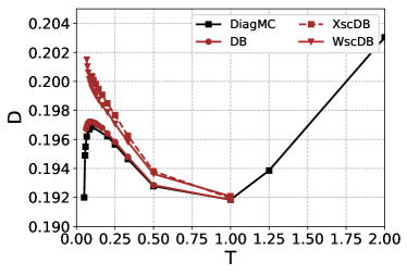
D.10 DB
The Dual Boson (DB) approach Rubtsov et al. (2012); van Loon et al. (2014a); Stepanov et al. (2016b) is an extension of the DF approach that additionally to the local Coulomb interaction accounts for the effect of nonlocal interactions in different bosonic channels (). Within the DB approach, local electronic correlations are considered exactly in the framework of the (extended) dynamical mean-field theory (EDMFT) Sun and Kotliar (2002, 2004). Nonlocal collective fluctuations are treated diagrammatically beyond the EDMFT level. For this aim, dual boson fields are introduced in addition to dual fermion variables that are already present in the DF approach. The DB theory is derived analytically using a path integral formalism, so many existing EDMFT-based approaches can be obtained as a certain approximation of the DB method Stepanov et al. (2019a, 2016b). Also, the DB theory fulfills the Mermin-Wagner theorem, which allows to avoid unphysical phase transitions in two dimensions Peters et al. (2019).
The action of the DB theory is following
| (63) |
Here, the bare fermion and boson propagators are given by nonlocal parts of EDMFT Green function and renormalized interaction Stepanov et al. (2016b), respectively.
The interaction part of the dual action contains all possible exact local fermion-fermion and fermion-boson vertex functions of the impurity problem. Here, as well as in most of DB approximations, we restrict ourselves to the lowest-order (two-particle) interaction terms that are given by the 4-leg fermion-fermion and 3-leg fermion-boson vertex functions. This truncation of the interaction allows to describe collective charge van Loon et al. (2014b); Stepanov et al. (2019b) and spin Stepanov et al. (2018, 2018) degrees of freedom in a conserving way using the ladder DB approximation Rubtsov et al. (2012); Stepanov et al. (2016b); van Loon et al. (2014a); Hafermann et al. (2014).
In the main part of the text only single-shot ladder Dual Boson results are discussed. These calculations are performed on the basis of the converged DMFT solution of the problem, where the bosonic hybridization function is equal to zero. Importantly, in the latter case the DB theory fully coincides with the DF approach if only the local Coulomb interaction is considered. The corresponding local impurity problem is solved using the open source CT-HYB solver Hafermann et al. (2013); Hafermann (2014) based on the ALPS libraries Bauer et al. (2011). This solution requires Monte Carlo steps. After that, we calculate the dual self-energy and polarization operator diagrammatically, and perform only the inner self-consistency loop in order to obtain the dressed Green’s function and renormalized interaction using the Dyson equation. For this, we use momentum grid with a maximum linear mesh size of , and the number of fermionic and bosonic Matsubara frequencies and , respectively. The expression for the lattice self-energy of the DB approach coincides with the one of the DF theory in Eq. (62). The lattice polarization function can be found using a similar expression Stepanov et al. (2016a):
| (64) |
The fully self-consistent DB calculations can be performed as follows. To obtain the fermionic hybridization of the effective impurity problem, we use the outer self-consistency condition that equates the local part of the lattice Green function and local impurity Green function . Regarding the bosonic hybridization function, there is no clear receipt how this quantity has to be determined. Here, we investigate two different self-consistency schemes that fix the bosonic hybridization. For the X-self-consistent (Xsc) result the local part of the lattice susceptibility is equated to the corresponding local susceptibility of the impurity problem . The other self-consistency can be imposed on a renormalized (screened) interaction (Wsc) . The renormalized interaction of the lattice problem can be defined as
| (65) |
where Stepanov et al. (2019a). The EDMFT renormalized interaction can be obtained neglecting the dual contribution to polarization operator in Eq. (65), so that . The renormalized interaction of the impurity problem can be found as
| (66) |
where is the bosonic hybridization function. Corresponding results are shown in Figs. 36 and 37. We note as well that the comparisons between self-consistent DB and self-consistent DF schemes are in good agreement, but differ from the exact result. As we point out in the main text, the single-shot DB approach correctly reproduces exact DiagMC results at almost all temperatures. Surprisingly, we observe that the Xsc DB calculations strongly deviate from the exact result presented in both Figures. At the same time, we find that the Wsc DB result for the self-energy agrees with DiagMC calculations even better than the single-shot DB one. However, two particle quantities, such as the lattice susceptibility and double occupancy, get worse when the self-consistency on the renormalized interaction is utilized. This can be explained by the fact that considered bosonic self-consistencies cannot fix all desired single- and two-particle quantities at the same time. Therefore, the question of a good self-consistency for the bosonic hybridization function remains open.
Other approximations
D.11 TPSC and TPSC+
D.11.1 TPSC
The two-particle self-consistent (TPSC) Vilk et al. (1994); Vilk (1995); Vilk and Tremblay (1996) approach is a nonperturbative approach that is only valid from weak to intermediate interaction strength; hence, it does not describe the Mott transition. Nevertheless, there are a large number of physical phenomena that it allows to study with an accuracy comparable to other numerically exact methods. In particular, in two dimensions, it describes the entry into the renormalized classical regime of antiferromagnetic fluctuations. There are no adjustable parameters as opposed to, for example, self-consistent renormalized spin-fluctuation theory. It satisfies conservation laws for total spin and total charge, the Mermin-Wagner theorem, the Pauli principle in the form , as well as the local spin and local charge sum rules. The two local sum rules in addition to the ansatz that the renormalized irreducible spin interaction vertex is given by suffice to obtain the irreducible vertices
| (67) |
and then compute the spin and charge susceptibilities from
| (68a) | ||||
| (68b) | ||||
The local spin and charge sum rules are given by and , respectively, and the trace is over the spin and momentum space. The above ansatz for is inspired from Ref. Singwi and Tosi, 1981; Ichimaru, 1982 and was found independently in Ref. Hedayati and Vignale, 1989.
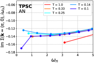
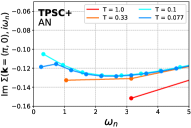
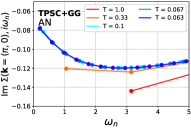
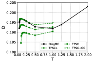
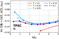
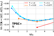
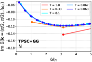
At the first-level approximation (hence the superscript “”) of TPSC, the irreducible particle-hole bubble diagram is obtained from
| (69) |
where the Green function includes a constant self-energy and renormalized chemical potential that lead to a non-interacting form . The two irreducible vertices suffice to find an improved self-energy Moukouri et al. (2000) that does not assume Migdal’s theorem and that takes into account rotational invariance and crossing symmetry
| (70) |
The consistency condition between one-particle and two-particle properties (Galitskii-Migdal formula referred in the main text)
| (71) |
serves as a guide for the domain of validity of TPSC. (Double occupancy obtained from sum rules on spin and charge equals that obtained from the self-energy and the Green function. When starts to deviate from the above, the method starts to fail.) See Vilk and Tremblay (1997); Allen et al. (2003) for detailed comparisons with QMC calculations and other approaches and discussions of the physics. Ref. Tremblay et al. (2006) reviews the work related to the pseudogap and superconductivity up to 2005 including detailed comparisons with quantum cluster approaches in the regime of validity that overlaps with TPSC (intermediate coupling). A pedagogical review of results and derivation appears in Ref. Tremblay (2011).
TPSC numerical results in the present paper have been obtained on a lattice and Matsubara frequencies with tails treated analytically. Due to the self-energy iterations, we use a lattice and Matsubara frequencies in TPSC+ calculations, so that the sufficient precision can be obtained using moderate computational resources, as in TPSC.
D.11.2 TPSC+
One of the main limitations of TPSC is that even for weak to intermediate interaction strength, it is not valid deep in the renormalized classical regime Vilk et al. (1994). For example, for the half-filled Hubbard model with only nearest-neighbor hopping, one finds that tends to zero as temperature goes to zero, contrary to the fact that and the site double occupancy must saturate to a finite value as due to virtual states.
To remedy this problem, an improved TPSC has recently been proposed Wang et al. . We refer to this extension as TPSC+. It is based on an extension of Kadanoff and Martin’s ideas Kadanoff and Martin (1961) who treated the normal state of superconductors in such a way that it connects smoothly to the superconducting state described by the BCS equation. The key idea is that the pair susceptibility takes an asymmetric form . It is called the pairing approximation or theory in this context and it has been extensively used by Levin’s group to study pairing pseudogap and related phenomena Chen et al. (2005); Boyack et al. (2018).
We apply that idea to the repulsive Hubbard model and use the asymmetric form in the particle-hole bubble
| (72) |
where the self-energy entering has the same form as Eq. (D.11.1): Contrary to the original Kadanoff-Martin approach, the irreducible vertices are computed from the same sum rules and ansatz but the susceptibilities in Eq. (68) are obtained from instead of from . The tilde symbol () indicates that , , and self-consistently depend on each other. Note that the trace also includes the spin.
The advantages of this approach are as follows. (a) The generalized Stoner criterion for the phase transition temperature becomes identical to the mean-field gap equation in the antiferromagnetic state with the interaction vertex reduced from the bare to Wang et al. .
(b) The Mermin-Wagner theorem and the Pauli principle are satisfied. Analytical arguments that demonstrate these results proceed in a manner analogous to those in TPSC. (c) One- and two-particle properties are consistent in the sense that is satisfied exactly with double-occupancy equal to that obtained from the local spin and charge sum rules. (d) Analytical arguments analogous to those in TPSC show that there is a pseudogap in two dimensions that is a precursor to the antiferromagnetically ordered state at zero temperature. Because the susceptibility dressed by self-energy remains finite at zero temperature, renormalized remains finite while pushing to zero. Furthermore, at zero temperature, the size of the pseudogap becomes equal to the finite magnetic gap .
On the down side, the susceptibilities at zero wave vector do not vanish at finite frequency, as conservation laws say they should. However, the values of the zero-wave vector susceptibilities at finite frequency are generally small. Finally, the -sum rule is also slightly violated.
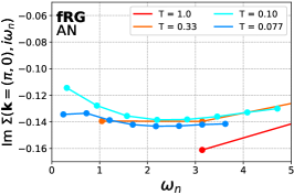
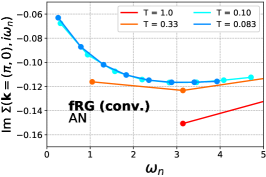
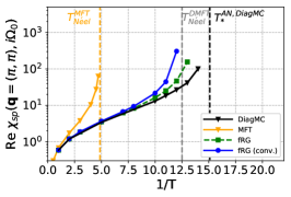
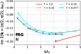
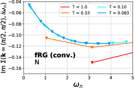
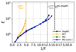
Heuristically, another explanation of the approach comes from the expected cancellations between vertices and self-energy. Consider the Bethe-Salpeter equation for the four-point function (susceptibilities)
| (73) |
where we have used the identity . Suppose a quasiparticle picture applies, namely where is the quasiparticle weight.
In some approximation, the from the vertices cancels from one of the Green functions. In some sense, and account for the average momentum-space screening of the interaction vertices while accounts for their frequency dependence.
Numerical results for TPSC+ in the present paper have been obtained on a lattice and Matsubara frequencies. Fast Fourier transforms with a uniform grid for imaginary time are used in the self-consistent calculations of and .
Eventually, we would like to comment on result from a TPSC+ variety, which utilizes the full Green function instead of and is therefore coined TPSC+GG. In Fig. 35 we already saw that there is a very good agreement of the TPSC+GG with DA for the spin susceptibility and correlation length. Fig. 38 now also shows that at low the double occupancy agrees well with the benchmark, although it does not open the pseudogap.
D.12 fRG
The characteristic scale-dependent behavior of numerous strongly correlated electron systems can be treated in a flexible and unbiased way by the functional renormalization group (fRG), see Refs. Metzner et al. (2012); Salmhofer (1999); Berges et al. (2002); Kopietz et al. (2010) for a review, (see also Deisz et al. (1996); Katanin and Kampf (2004); Rohe and Metzner (2005); Kampf and Katanin (2006) for the context of the pseudogap). Its starting point is an exact functional flow equation, which yields the gradual evolution from a microscopic model action to the final effective action as a function of a continuously decreasing energy scale. Expanding in powers of the fields one obtains an exact hierarchy of flow equations for the -particle irreducible vertex functions, which in practical implementations is truncated at the two-particle level.
| 1 | 4 | 8 | 15 | 40 |
|---|---|---|---|---|
| 2 | 4 | 8 | 15 | 40 |
| 3 | 4 | 8 | 15 | 40 |
| 5 | 6 | 12 | 15 | 60 |
| 7 | 8 | 16 | 15 | 80 |
| 8 | 8 | 16 | 15 | 80 |
| 10 | 8 | 16 | 15 | 80 |
| 11 | 8 | 16 | 15 | 80 |
| 12 | 8 | 16 | 15 | 80 |
| 13 | 8 | 20 | 15 | 100 |
Neglecting the renormalization of three- and higher order particle vertices yields approximate 1-loop flow equations for the self-energy and two-particle vertex 222Strongly correlated parameter regimes are beyond the 1-loop flow but might become accessible by exploiting the DMFT as a starting point for the fRG flow Taranto et al. (2014); Vilardi et al. (2019)..
The underlying approximations are devised for the weak to moderate coupling regime. A substantial improvement with respect to previous fRG-based computation schemes relies on an efficient parametrization of the two-particle vertex, where we combine the so-called ”truncated unity” fRG Husemann and Salmhofer (2009); Wang et al. (2012); Lichtenstein et al. (2017) using the channel decomposition in conjunction with a form factor expansion for the momentum dependence with the full frequency treatment Vilardi et al. (2017) that includes the high-frequency asymptotics Rohringer et al. (2012); Wentzell et al. (2020). We here use the Katanin replacement Katanin (2004) in the flow equation for the two-particle vertex as a first step towards the multiloop extension of the fRG which would allow to sum up all the diagrams of the parquet approximation with their exact weight Kugler and von Delft (2018c, b); Tagliavini et al. (2019). In order to account for the form-factor truncation, the self-energy flow is determined by the scale derivative of the Schwinger-Dyson equation Hille et al. (2020a, b) replacing the conventional one-loop flow equation (in Fig. 39). We refer to Refs. Hille et al. (2020a, b); Tagliavini et al. (2019) for the details of the algorithmic implementation and in particular also for the post-processed computation of the susceptibilities from the flowing vertex and self-energy, the technical parameters are reported in Tab. 2. The double occupancy was calculated from two-particle quantities according to
| (74) |
We note that taking into account also multiloop corrections, these algorithmic advancements have been shown to bring the fRG for interacting fermions on 2D lattices to a quantitatively reliable level, in particular recovering the PA Hille et al. (2020a); Tagliavini et al. (2019).
D.13 PA
The parquet approach is a diagrammatic scheme first introduced by DeDominicis and Martin in 1964 De Dominicis and Martin (1964a). It relies on the classification of diagrams contributing to the full 1-particle irreducible 2-particle vertex in terms of their 2-particle reducibility. These diagrams can be either fully 2-particle irreducible or 2-particle reducible in one of three channels De Dominicis and Martin (1964b); Bickers (2004); Vasil’ev et al. (1974). The method is unbiased with respect to the channels and exact if using the exact fully 2-particle irreducible vertex as an input.
The parquet approximation (PA) applied here, consists in setting this fully 2-particle irreducible vertex to the bare Hubbard i.e. its lowest order contribution. This is correct only up to fourth order in perturbation theory. The PA has previously been used to study several condensed matter problems including the Hubbard model Yang et al. (2009); Tam et al. (2013); Kauch et al. (2019, 2020); Li et al. (2019); Pudleiner et al. (2019a, b). The here presented results have been obtained with the TUPS Eckhardt et al. (2020) implementation which relies on the method of Truncated Unities Lichtenstein et al. (2017); Eckhardt et al. (2018) and vertex asymptotics Wentzell et al. (2020); Li et al. (2016) in order to represent vertex functions as well as a previously developed parallelization scheme in order to perform computations efficiently Tam et al. (2013); Li et al. (2019).
All results are converged in the number of discrete lattice momenta (Nq) and positive fermionic Matsubara frequencies (Nf+) used. Concretely we use a linear mesh size of and at and fewer frequencies and momenta for higher temperatures. The results for have been extrapolated to in
finite momentum grid size. The number of basis functions () inherent to the Truncated Unity method Eckhardt et al. (2018) was set to for all calculations. As has been shown in Eckhardt et al. (2018) it is sufficient to reproduce the full basis results for but constitutes an additional approximation for lower temperatures. This approximation is quite likely responsible for the PA underestimation of AFM susceptibility (and, as a consequence, the pseudogap temperature) in comparison with the benchmark. The AFM susceptibility is also underestimated in the full parquet DA scheme, when the number of basis functions is limited to , as has been shown in Kaufmann et al. (2021). A very promising new computational scheme has recently been proposed Krien et al. (2021) that may allow for significant reduction of frequency box sizes and thus make computations with more basis functions () feasible. The double occupancy was calculated using Eq. (8). Please note, that in the PA the sum rule relating the double occupancy obtained from one-particle and two-particle quantities
| (75) | |||||
is fulfilled by construction. The PA also fulfills Bickers and Scalapino (1992); Eckhardt et al. (2020) the Mermin-Wagner theorem Mermin and Wagner (1966); Hohenberg (1967).
References
- Hubbard (1963) J. Hubbard, “Electron Correlations in Narrow Energy Bands,” Proceedings of the Royal Society of London. Series A, Mathematical and Physical Sciences 276, 238–257 (1963).
- Hubbard (1964) J. Hubbard, “Electron Correlations in Narrow Energy Bands. III. An Improved Solution,” Proc R. Soc. London 281, 401–419 (1964).
- Gutzwiller (1963) Martin C. Gutzwiller, “Effect of Correlation on the Ferromagnetism of Transition Metals,” Phys. Rev. Lett. 10, 159–162 (1963).
- Kanamori (1963) Junjiro Kanamori, “Electron Correlation and Ferromagnetism of Transition Metals,” Progress of Theoretical Physics 30, 275–289 (1963), https://academic.oup.com/ptp/article-pdf/30/3/275/5278869/30-3-275.pdf .
- Jaksch and Zoller (2005) D. Jaksch and P. Zoller, “The cold atom Hubbard toolbox,” Annals of Physics 315, 52 – 79 (2005), special Issue.
- Bloch (2005) Immanuel Bloch, “Ultracold quantum gases in optical lattices,” Nature Physics 1, 23–30 (2005).
- Lewenstein et al. (2007) Maciej Lewenstein, Anna Sanpera, Veronica Ahufinger, Bogdan Damski, Aditi Sen(De), and Ujjwal Sen, “Ultracold atomic gases in optical lattices: mimicking condensed matter physics and beyond,” Advances in Physics 56, 243–379 (2007).
- Essler et al. (2005) F. H. L. Essler, H. Frahm, F. Göhmann, A. Klümper, and V. Korepin, The One-Dimensional Hubbard model (Cambridge University Press, 2005).
- Metzner and Vollhardt (1989) Walter Metzner and Dieter Vollhardt, “Correlated Lattice Fermions in Dimensions,” Phys. Rev. Lett. 62, 324–327 (1989).
- Georges and Kotliar (1992) Antoine Georges and Gabriel Kotliar, “Hubbard model in infinite dimensions,” Phys. Rev. B 45, 6479–6483 (1992).
- Jarrell (1992) M. Jarrell, “Hubbard model in infinite dimensions: A quantum Monte Carlo study,” Phys. Rev. Lett. 69, 168–171 (1992).
- Keimer et al. (2015) B. Keimer, S. A. Kivelson, M. R. Norman, S. Uchida, and J. Zaanen, “From quantum matter to high-temperature superconductivity in copper oxides,” Nature (London) 518, 179–186 (2015).
- Timusk and Statt (1999) Tom Timusk and Bryan Statt, “The pseudogap in high-temperature superconductors: an experimental survey,” Reports on Progress in Physics 62, 61–122 (1999).
- Norman et al. (2005) M. R. Norman, D. Pines, and C. Kallin, “The pseudogap: friend or foe of high Tc?” Advances in Physics 54, 715–733 (2005), arXiv:cond-mat/0507031 [cond-mat.supr-con] .
- Lee et al. (2006) Patrick A. Lee, Naoto Nagaosa, and Xiao-Gang Wen, “Doping a Mott insulator: Physics of high-temperature superconductivity,” Rev. Mod. Phys. 78, 17–85 (2006).
- LeBlanc et al. (2015) J. P. F. LeBlanc, Andrey E. Antipov, Federico Becca, Ireneusz W. Bulik, Garnet Kin-Lic Chan, Chia-Min Chung, Youjin Deng, Michel Ferrero, Thomas M. Henderson, Carlos A. Jiménez-Hoyos, E. Kozik, Xuan-Wen Liu, Andrew J. Millis, N. V. Prokof’ev, Mingpu Qin, Gustavo E. Scuseria, Hao Shi, B. V. Svistunov, Luca F. Tocchio, I. S. Tupitsyn, Steven R. White, Shiwei Zhang, Bo-Xiao Zheng, Zhenyue Zhu, and Emanuel Gull (Simons Collaboration on the Many-Electron Problem), “Solutions of the Two-Dimensional Hubbard Model: Benchmarks and Results from a Wide Range of Numerical Algorithms,” Phys. Rev. X 5, 041041 (2015).
- Motta et al. (2017) Mario Motta, David M. Ceperley, Garnet Kin-Lic Chan, John A. Gomez, Emanuel Gull, Sheng Guo, Carlos A. Jiménez-Hoyos, Tran Nguyen Lan, Jia Li, Fengjie Ma, Andrew J. Millis, Nikolay V. Prokof’ev, Ushnish Ray, Gustavo E. Scuseria, Sandro Sorella, Edwin M. Stoudenmire, Qiming Sun, Igor S. Tupitsyn, Steven R. White, Dominika Zgid, and Shiwei Zhang (Simons Collaboration on the Many-Electron Problem), “Towards the Solution of the Many-Electron Problem in Real Materials: Equation of State of the Hydrogen Chain with State-of-the-Art Many-Body Methods,” Phys. Rev. X 7, 031059 (2017).
- Williams et al. (2020) Kiel T. Williams, Yuan Yao, Jia Li, Li Chen, Hao Shi, Mario Motta, Chunyao Niu, Ushnish Ray, Sheng Guo, Robert J. Anderson, Junhao Li, Lan Nguyen Tran, Chia-Nan Yeh, Bastien Mussard, Sandeep Sharma, Fabien Bruneval, Mark van Schilfgaarde, George H. Booth, Garnet Kin-Lic Chan, Shiwei Zhang, Emanuel Gull, Dominika Zgid, Andrew Millis, Cyrus J. Umrigar, and Lucas K. Wagner (Simons Collaboration on the Many-Electron Problem), “Direct Comparison of Many-Body Methods for Realistic Electronic Hamiltonians,” Phys. Rev. X 10, 011041 (2020).
- Neronov (2019) Andrii Neronov, “Introduction to multi-messenger astronomy,” Journal of Physics: Conference Series 1263, 012001 (2019).
- Slater (1951) J. C. Slater, “Magnetic Effects and the Hartree-Fock Equation,” Phys. Rev. 82, 538–541 (1951).
- Mermin and Wagner (1966) N. D. Mermin and H. Wagner, “Absence of Ferromagnetism or Antiferromagnetism in One- or Two-Dimensional Isotropic Heisenberg Models,” Phys. Rev. Lett. 17, 1307–1307 (1966).
- Hohenberg (1967) P. C. Hohenberg, “Existence of Long-Range Order in One and Two Dimensions,” Phys. Rev. 158, 383–386 (1967).
- Blankenbecler et al. (1981) R. Blankenbecler, D. J. Scalapino, and R. L. Sugar, “Monte Carlo calculations of coupled boson-fermion systems. I,” Phys. Rev. D 24, 2278–2286 (1981).
- Prokof’ev and Svistunov (1998) Nikolai V. Prokof’ev and Boris V. Svistunov, “Polaron Problem by Diagrammatic Quantum Monte Carlo,” Phys. Rev. Lett. 81, 2514–2517 (1998).
- Rossi (2017) Riccardo Rossi, “Determinant Diagrammatic Monte Carlo Algorithm in the Thermodynamic Limit,” Phys. Rev. Lett. 119, 045701 (2017).
- Šimkovic and Kozik (2019) Fedor Šimkovic and Evgeny Kozik, “Determinant Monte Carlo for irreducible Feynman diagrams in the strongly correlated regime,” Phys. Rev. B 100, 121102(R) (2019).
- Moutenet et al. (2018) Alice Moutenet, Wei Wu, and Michel Ferrero, “Determinant Monte Carlo algorithms for dynamical quantities in fermionic systems,” Phys. Rev. B 97, 085117 (2018).
- Georges et al. (1996) Antoine Georges, Gabriel Kotliar, Werner Krauth, and Marcelo J. Rozenberg, “Dynamical mean-field theory of strongly correlated fermion systems and the limit of infinite dimensions,” Rev. Mod. Phys. 68, 13 (1996).
- Maier et al. (2005a) T. A. Maier, M. Jarrell, T. Pruschke, and M. Hettler, “Quantum Cluster Theories,” Rev. Mod. Phys. 77, 1027 (2005a).
- Kotliar et al. (2006) G. Kotliar, S. Y. Savrasov, K. Haule, V. S. Oudovenko, O. Parcollet, and C. A. Marianetti, “Electronic structure calculations with dynamical mean-field theory,” Rev. Mod. Phys. 78, 865 (2006).
- Tremblay et al. (2006) A. M. S. Tremblay, B. Kyung, and D. Sénéchal, “Pseudogap and high-temperature superconductivity from weak to strong coupling. towards a quantitative theory,” Low Temp. Phys. 32, 424–451 (2006).
- Lichtenstein and Katsnelson (2000) A. I. Lichtenstein and M. I. Katsnelson, “Antiferromagnetism and d-wave superconductivity in cuprates: A cluster dynamical mean-field theory,” Phys. Rev. B 62, R9283–R9286 (2000).
- Rohringer et al. (2018a) G. Rohringer, H. Hafermann, A. Toschi, A. A. Katanin, A. E. Antipov, M. I. Katsnelson, A. I. Lichtenstein, A. N. Rubtsov, and K. Held, “Diagrammatic routes to nonlocal correlations beyond dynamical mean field theory,” Rev. Mod. Phys. 90, 025003 (2018a).
- Vilk and Tremblay (1997) Y. M. Vilk and A.-M. S. Tremblay, “Non-Perturbative Many-Body Approach to the Hubbard Model and Single-Particle Pseudogap,” J. Phys. I France 7, 1309–1368 (1997).
- Tremblay (2011) A. M. S. Tremblay, “Two-particle-Self-Consistent Approach for the Hubbard model,” in Strongly Correlated Systems: Theoretical Methods, edited by F. Mancini and A. Avella (Springer series, 2011) Chap. 13, pp. 409–455.
- (36) Y. Wang, Y.M. Vilk, and A.-M. S. Tremblay, “An improved two-particle self-consistent approach,” To be published .
- Metzner et al. (2012) Walter Metzner, Manfred Salmhofer, Carsten Honerkamp, Volker Meden, and Kurt Schönhammer, “Functional renormalization group approach to correlated fermion systems,” Rev. Mod. Phys. 84, 299–352 (2012).
- De Dominicis and Martin (1964a) Cyrano De Dominicis and Paul C. Martin, “Stationary entropy principle and renormalization in normal and superfluid systems. II. diagrammatic formulation,” J. Math. Phys. 5, 31 (1964a).
- Bickers (2004) N. E. Bickers, “Theoretical methods for strongly correlated electrons,” (Springer-Verlag New York Berlin Heidelbert, 2004) Chap. 6, pp. 237–296.
- White (2009) Steven R. White, “Minimally Entangled Typical Quantum States at Finite Temperature,” Phys. Rev. Lett. 102, 190601 (2009).
- Stoudenmire and White (2010) E M Stoudenmire and Steven R White, “Minimally entangled typical thermal state algorithms,” New Journal of Physics 12, 055026 (2010).
- Bruognolo et al. (2015) Benedikt Bruognolo, Jan von Delft, and Andreas Weichselbaum, “Symmetric minimally entangled typical thermal states,” Phys. Rev. B 92, 115105 (2015).
- Wietek et al. (2020) Alexander Wietek, Yuan-Yao He, Steven R. White, Antoine Georges, and E. Miles Stoudenmire, “Stripes, Antiferromagnetism, and the Pseudogap in the Doped Hubbard Model at Finite Temperature,” (2020), arXiv:2009.10736 [cond-mat.str-el] .
- Wietek et al. (2021) Alexander Wietek, Riccardo Rossi, Fedor Šimkovic IV, Marcel Klett, Philipp Hansmann, Michel Ferrero, E. Miles Stoudenmire, Thomas Schäfer, and Antoine Georges, “Mott insulating states with competing orders in the triangular lattice Hubbard model,” (2021), arXiv:2102.12904 [cond-mat.str-el] .
- (45) See Supplemental Material available under this link.
- Katanin et al. (2009) A. A. Katanin, A. Toschi, and K. Held, “Comparing pertinent effects of antiferromagnetic fluctuations in the two- and three-dimensional Hubbard model,” Phys. Rev. B 80, 075104 (2009).
- Rohringer and Toschi (2016) G. Rohringer and A. Toschi, “Impact of non-local correlations over different energy scales: A Dynamical Vertex Approximation study,” Phys. Rev. B 94, 125144 (2016).
- Rohringer and Toschi (2020) G. Rohringer and A. Toschi, private communication (2020).
- Baier et al. (2004) Tobias Baier, Eike Bick, and Christof Wetterich, “Temperature dependence of antiferromagnetic order in the Hubbard model,” Phys. Rev. B 70, 125111 (2004).
- Kugler and von Delft (2018a) Fabian B. Kugler and Jan von Delft, “Multiloop Functional Renormalization Group That Sums Up All Parquet Diagrams,” Phys. Rev. Lett. 120, 057403 (2018a).
- Kugler and von Delft (2018b) Fabian B. Kugler and Jan von Delft, “Multiloop functional renormalization group for general models,” Phys. Rev. B 97, 35162 (2018b), arXiv:1703.06505 .
- Hille et al. (2020a) Cornelia Hille, Fabian B. Kugler, Christian J. Eckhardt, Yuan-Yao He, Anna Kauch, Carsten Honerkamp, Alessandro Toschi, and Sabine Andergassen, “Quantitative functional renormalization group description of the two-dimensional Hubbard model,” Phys. Rev. Research 2, 033372 (2020a).
- Hille et al. (2020b) Cornelia Hille, Daniel Rohe, Carsten Honerkamp, and Sabine Andergassen, “Pseudogap opening in the two-dimensional Hubbard model: A functional renormalization group analysis,” Phys. Rev. Research 2, 033068 (2020b).
- Bickers and Scalapino (1992) N. E. Bickers and D. J. Scalapino, “Critical behavior of electronic parquet solutions,” Phys. Rev. B 46, 8050–8056 (1992).
- Eckhardt et al. (2018) C. J. Eckhardt, G. A. H. Schober, J. Ehrlich, and C. Honerkamp, “Truncated-unity parquet equations: Application to the repulsive Hubbard model,” Phys. Rev. B 98, 075143 (2018).
- Eckhardt et al. (2020) Christian J. Eckhardt, Carsten Honerkamp, Karsten Held, and Anna Kauch, “Truncated unity parquet solver,” Phys. Rev. B 101, 155104 (2020).
- Schäfer et al. (2015a) T. Schäfer, F. Geles, D. Rost, G. Rohringer, E. Arrigoni, K. Held, N. Blümer, M. Aichhorn, and A. Toschi, “Fate of the false Mott-Hubbard transition in two dimensions,” Phys. Rev. B 91, 125109 (2015a).
- Šimkovic et al. (2020) Fedor Šimkovic, J. P. F. LeBlanc, Aaram J. Kim, Youjin Deng, N. V. Prokof’ev, B. V. Svistunov, and Evgeny Kozik, “Extended Crossover from a Fermi Liquid to a Quasiantiferromagnet in the Half-Filled 2D Hubbard Model,” Phys. Rev. Lett. 124, 017003 (2020).
- Kim et al. (2020) Aaram J. Kim, Fedor Simkovic, and Evgeny Kozik, “Spin and Charge Correlations across the Metal-to-Insulator Crossover in the Half-Filled 2D Hubbard Model,” Phys. Rev. Lett. 124, 117602 (2020).
- Tanaka (2019) Arata Tanaka, “Metal-insulator transition in the two-dimensional Hubbard model: Dual fermion approach with Lanczos exact diagonalization,” Phys. Rev. B 99, 205133 (2019).
- Schäfer et al. (2016a) T. Schäfer, A. Toschi, and K. Held, “Dynamical vertex approximation for the two-dimensional Hubbard model,” Journal of Magnetism and Magnetic Materials 400, 107–111 (2016a).
- Rost et al. (2012) D. Rost, E. V. Gorelik, F. Assaad, and N. Blümer, “Momentum-dependent pseudogaps in the half-filled two-dimensional Hubbard model,” Phys. Rev. B 86, 155109 (2012).
- Rost and Blümer (2015) D Rost and N Blümer, “Deciding the fate of the false Mott transition in two dimensions by exact quantum Monte Carlo methods,” Journal of Physics: Conference Series 640, 012047 (2015).
- Sangiovanni et al. (2006) G. Sangiovanni, A. Toschi, E. Koch, K. Held, M. Capone, C. Castellani, O. Gunnarsson, S.-K. Mo, J. W. Allen, H.-D. Kim, A. Sekiyama, A. Yamasaki, S. Suga, and P. Metcalf, “Static versus dynamical mean-field theory of Mott antiferromagnets,” Phys. Rev. B 73, 205121 (2006).
- Parisi (1998) Giorgio Parisi, Statistical Field Theory (CRC Press (Advanced Book Classics, 1998).
- Hettler et al. (1998) M. H. Hettler, A. N. Tahvildar-Zadeh, M. Jarrell, T. Pruschke, and H. R. Krishnamurthy, “Nonlocal dynamical correlations of strongly interacting electron systems,” Phys. Rev. B 58, R7475–R7479 (1998).
- Hettler et al. (2000) M. H. Hettler, M. Mukherjee, M. Jarrell, and H. R. Krishnamurthy, “Dynamical cluster approximation: Nonlocal dynamics of correlated electron systems,” Phys. Rev. B 61, 12739–12756 (2000).
- Aryanpour et al. (2002) K. Aryanpour, M. H. Hettler, and M. Jarrell, “Analysis of the dynamical cluster approximation for the Hubbard model,” Phys. Rev. B 65, 153102 (2002).
- Kotliar et al. (2001) Gabriel Kotliar, Sergej Y. Savrasov, Gunnar Pálsson, and Giulio Biroli, “Cellular Dynamical Mean Field Approach to Strongly Correlated Systems,” Phys. Rev. Lett. 87, 186401 (2001).
- Klett et al. (2020) Marcel Klett, Nils Wentzell, Thomas Schäfer, Fedor Simkovic, Olivier Parcollet, Sabine Andergassen, and Philipp Hansmann, “Real-space cluster dynamical mean-field theory: Center-focused extrapolation on the one- and two particle-levels,” Phys. Rev. Research 2, 033476 (2020).
- Rohringer et al. (2011) G. Rohringer, A. Toschi, A. Katanin, and K. Held, “Critical Properties of the Half-Filled Hubbard Model in Three Dimensions,” Phys. Rev. Lett. 107, 256402 (2011).
- Gull et al. (2008a) E. Gull, P. Werner, X. Wang, M. Troyer, and A. J. Millis, “Local order and the gapped phase of the Hubbard model: A plaquette dynamical mean-field investigation,” EPL (Europhysics Letters) 84, 37009 (2008a).
- Gull et al. (2009) Emanuel Gull, Olivier Parcollet, Philipp Werner, and Andrew J. Millis, “Momentum-sector-selective metal-insulator transition in the eight-site dynamical mean-field approximation to the Hubbard model in two dimensions,” Phys. Rev. B 80, 245102 (2009).
- Gull et al. (2010) E. Gull, M. Ferrero, O. Parcollet, A. Georges, and A. J. Millis, “Momentum-space anisotropy and pseudogaps: A comparative cluster dynamical mean-field analysis of the doping-driven metal-insulator transition in the two-dimensional Hubbard model,” Phys. Rev. B 82, 155101 (2010).
- Gull et al. (2013) Emanuel Gull, Olivier Parcollet, and Andrew J. Millis, “Superconductivity and the Pseudogap in the Two-Dimensional Hubbard Model,” Phys. Rev. Lett. 110, 216405 (2013).
- Parcollet et al. (2004) O. Parcollet, G. Biroli, and G. Kotliar, “Cluster Dynamical Mean Field Analysis of the Mott Transition,” Phys. Rev. Lett. 92, 226402 (2004).
- Macridin et al. (2006) Alexandru Macridin, M. Jarrell, Thomas Maier, P. R. C. Kent, and Eduardo D’Azevedo, “Pseudogap and Antiferromagnetic Correlations in the Hubbard Model,” Phys. Rev. Lett. 97, 036401 (2006).
- Sénéchal and Tremblay (2004) David Sénéchal and A.-M. S. Tremblay, “Hot Spots and Pseudogaps for Hole- and Electron-Doped High-Temperature Superconductors,” Phys. Rev. Lett. 92, 126401 (2004).
- Haule and Kotliar (2007) Kristjan Haule and Gabriel Kotliar, “Strongly correlated superconductivity: A plaquette dynamical mean-field theory study,” Phys. Rev. B 76, 104509 (2007).
- Park et al. (2008) H. Park, K. Haule, and G. Kotliar, “Cluster Dynamical Mean Field Theory of the Mott Transition,” Phys. Rev. Lett. 101, 186403 (2008).
- Ferrero et al. (2009a) Michel Ferrero, Pablo S. Cornaglia, Lorenzo De Leo, Olivier Parcollet, Gabriel Kotliar, and Antoine Georges, “Pseudogap opening and formation of Fermi arcs as an orbital-selective Mott transition in momentum space,” Phys. Rev. B 80, 064501 (2009a).
- Ferrero et al. (2009b) M. Ferrero, P. S. Cornaglia, L. De Leo, O. Parcollet, G. Kotliar, and A. Georges, “Valence bond dynamical mean-field theory of doped Mott insulators with nodal/antinodal differentiation,” EPL (Europhysics Letters) 85, 57009 (2009b).
- Werner et al. (2009) Philipp Werner, Emanuel Gull, Olivier Parcollet, and Andrew J. Millis, “Momentum-selective metal-insulator transition in the two-dimensional Hubbard model: An 8-site dynamical cluster approximation study,” Phys. Rev. B 80, 045120 (2009).
- Sordi et al. (2012a) G. Sordi, P. Sémon, K. Haule, and A.-M. S. Tremblay, “Strong Coupling Superconductivity, Pseudogap, and Mott Transition,” Phys. Rev. Lett. 108, 216401 (2012a).
- Sordi et al. (2012b) G Sordi, P Sémon, Kristjan Haule, and A-MS Tremblay, “Pseudogap temperature as a Widom line in doped Mott insulators,” Scientific reports 2, 1–5 (2012b).
- Sordi et al. (2013) G. Sordi, P. Sémon, K. Haule, and A.-M. S. Tremblay, “-axis resistivity, pseudogap, superconductivity, and widom line in doped mott insulators,” Phys. Rev. B 87, 041101(R) (2013).
- Gunnarsson et al. (2015) O. Gunnarsson, T. Schäfer, J. P. F. LeBlanc, E. Gull, J. Merino, G. Sangiovanni, G. Rohringer, and A. Toschi, “Fluctuation Diagnostics of the Electron Self-Energy: Origin of the Pseudogap Physics,” Phys. Rev. Lett. 114, 236402 (2015).
- Wu et al. (2018) Wei Wu, Mathias S. Scheurer, Shubhayu Chatterjee, Subir Sachdev, Antoine Georges, and Michel Ferrero, “Pseudogap and Fermi-Surface Topology in the Two-Dimensional Hubbard Model,” Phys. Rev. X 8, 021048 (2018).
- Scheurer et al. (2018) Mathias S. Scheurer, Shubhayu Chatterjee, Wei Wu, Michel Ferrero, Antoine Georges, and Subir Sachdev, “Topological order in the pseudogap metal,” Proceedings of the National Academy of Sciences 115, E3665–E3672 (2018), https://www.pnas.org/content/115/16/E3665.full.pdf .
- Reymbaut et al. (2019) A. Reymbaut, S. Bergeron, R. Garioud, M. Thénault, M. Charlebois, P. Sémon, and A.-M. S. Tremblay, “Pseudogap, van Hove singularity, maximum in entropy, and specific heat for hole-doped Mott insulators,” Phys. Rev. Research 1, 023015 (2019).
- Fratino et al. (2017) L. Fratino, P. Sémon, M. Charlebois, G. Sordi, and A.-M. S. Tremblay, “Signatures of the Mott transition in the antiferromagnetic state of the two-dimensional Hubbard model,” Phys. Rev. B 95, 235109 (2017).
- Vilk (1995) Y. Vilk, “Destruction of the Fermi liquid by spin fluctuations in two dimensions,” Journal of Physics and Chemistry of Solids 56, 1769–1771 (1995).
- Vilk and Tremblay (1996) Y. M. Vilk and A.-M. S. Tremblay, “Destruction of Fermi-liquid quasiparticles in two dimensions by critical fluctuations,” EPL (Europhysics Letters) 33, 159 (1996).
- Georges and Krauth (1993) Antoine Georges and Werner Krauth, “Physical properties of the half-filled Hubbard model in infinite dimensions,” Phys. Rev. B 48, 7167–7182 (1993).
- Werner et al. (2005) F. Werner, O. Parcollet, A. Georges, and S. R. Hassan, “Interaction-Induced Adiabatic Cooling and Antiferromagnetism of Cold Fermions in Optical Lattices,” Phys. Rev. Lett. 95, 056401 (2005).
- Daré et al. (2007) A.-M. Daré, L. Raymond, G. Albinet, and A.-M. S. Tremblay, “Interaction-induced adiabatic cooling for antiferromagnetism in optical lattices,” Phys. Rev. B 76, 064402 (2007).
- Taie et al. (2012) Shintaro Taie, Rekishu Yamazaki, Seiji Sugawa, and Yoshiro Takahashi, “An SU(6) Mott insulator of an atomic Fermi gas realized by large-spin Pomeranchuk cooling,” Nature Physics 8, 825–830 (2012), arXiv:1208.4883 [cond-mat.quant-gas] .
- Galitskii and Migdal (1958) V. M. Galitskii and A. B. Migdal, “Application of quantum fiel theoretical methods to the many-body problem,” Sov. Phys. JETP 34, 139 (1958).
- van Loon et al. (2016) Erik G. C. P. van Loon, Friedrich Krien, Hartmut Hafermann, Evgeny A. Stepanov, Alexander I. Lichtenstein, and Mikhail I. Katsnelson, “Double occupancy in dynamical mean-field theory and the dual boson approach,” Phys. Rev. B 93, 155162 (2016).
- Chakravarty et al. (1988) Sudip Chakravarty, Bertrand I. Halperin, and David R. Nelson, “Low-temperature behavior of two-dimensional quantum antiferromagnets,” Phys. Rev. Lett. 60, 1057–1060 (1988).
- Chakravarty et al. (1989) Sudip Chakravarty, Bertrand I. Halperin, and David R. Nelson, “Two-dimensional quantum Heisenberg antiferromagnet at low temperatures,” Phys. Rev. B 39, 2344–2371 (1989).
- Borejsza and Dupuis (2003) K. Borejsza and N. Dupuis, “Antiferromagnetism and single-particle properties in the two-dimensional half-filled Hubbard model: Slater vs. Mott-Heisenberg,” Europhys. Lett. 63, 722–728 (2003).
- Borejsza and Dupuis (2004) K. Borejsza and N. Dupuis, “Antiferromagnetism and single-particle properties in the two-dimensional half-filled Hubbard model: A nonlinear sigma model approach,” Phys. Rev. B 69, 085119 (2004).
- Maier et al. (2005b) T. A. Maier, M. Jarrell, T. C. Schulthess, P. R. C. Kent, and J. B. White, “Systematic Study of -Wave Superconductivity in the 2D Repulsive Hubbard Model,” Phys. Rev. Lett. 95, 237001 (2005b).
- Toschi et al. (2007) A. Toschi, A. A. Katanin, and K. Held, “Dynamical vertex approximation; a step beyond dynamical mean-field theory,” Phys Rev. B 75, 045118 (2007).
- Wentzell et al. (2020) Nils Wentzell, Gang Li, Agnese Tagliavini, Ciro Taranto, Georg Rohringer, Karsten Held, Alessandro Toschi, and Sabine Andergassen, “High-frequency asymptotics of the vertex function: Diagrammatic parametrization and algorithmic implementation,” Phys. Rev. B 102, 085106 (2020).
- Kaufmann et al. (2017) Josef Kaufmann, Patrik Gunacker, and Karsten Held, “Continuous-time quantum Monte Carlo calculation of multiorbital vertex asymptotics,” Phys. Rev. B 96, 035114 (2017).
- Katanin (2020) A. Katanin, “Improved treatment of fermion-boson vertices and Bethe-Salpeter equations in nonlocal extensions of dynamical mean field theory,” Phys. Rev. B 101, 035110 (2020).
- Ornstein and Zernike (1916) L. S. Ornstein and F. Zernike, Proc. Roy. Acad. Amsterdam 17, 793 (1916).
- Moukouri et al. (2000) S. Moukouri, S. Allen, F. Lemay, B. Kyung, D. Poulin, Y. M. Vilk, and A.-M. S. Tremblay, “Many-body theory versus simulations for the pseudogap in the Hubbard model,” Phys. Rev. B 61, 7887–7892 (2000).
- Sedrakyan and Chubukov (2010) Tigran A. Sedrakyan and Andrey V. Chubukov, “Pseudogap in underdoped cuprates and spin-density-wave fluctuations,” Phys. Rev. B 81, 174536 (2010).
- Vilk (1997) Y. M. Vilk, “Shadow features and shadow bands in the paramagnetic state of cuprate superconductors,” Phys. Rev. B 55, 3870–3875 (1997).
- Lemay (2000) François Lemay, Des propriétés de l’état normal du modèle de Hubbard bidimensionnel, Ph.D. thesis, Université de Sherbrooke (2000).
- Zlatic (1997) V Zlatic, “Temperature dependence of the spectral properties for 2-D Hubbard model with anisotropic hopping,” PHYSICA B 230, 1034–1036 (1997).
- Katanin et al. (2005) A. A. Katanin, A. P. Kampf, and V. Yu. Irkhin, “Anomalous self-energy and Fermi surface quasisplitting in the vicinity of a ferromagnetic instability,” Phys. Rev. B 71, 085105 (2005).
- Müller-Hartmann (1989) E. Müller-Hartmann, “The Hubbard model at high dimensions: some exact results and weak coupling theory,” Zeitschrift fur Physik B Condensed Matter 76, 211–217 (1989).
- Ku and Eguiluz (2002) Wei Ku and Adolfo G. Eguiluz, “Band-gap problem in semiconductors revisited: Effects of core states and many-body self-consistency,” Phys. Rev. Lett. 89, 126401 (2002).
- Delaney et al. (2004) Kris Delaney, P. García-González, Angel Rubio, Patrick Rinke, and R. W. Godby, “Comment on “band-gap problem in semiconductors revisited: Effects of core states and many-body self-consistency”,” Phys. Rev. Lett. 93, 249701 (2004).
- Ku and Eguiluz (2004) Wei Ku and A. G. Eguiluz, “Ku and Eguiluz Reply,” Phys. Rev. Lett. 93, 249702 (2004).
- Prokof’ev and Svistunov (2007) Nikolay Prokof’ev and Boris Svistunov, “Bold Diagrammatic Monte Carlo Technique: When the Sign Problem Is Welcome,” Phys. Rev. Lett. 99, 250201 (2007).
- Deng et al. (2015) Youjin Deng, Evgeny Kozik, Nikolay V. Prokof’ev, and Boris V. Svistunov, “Emergent BCS regime of the two-dimensional fermionic Hubbard model: Ground-state phase diagram,” EPL (Europhysics Letters) 110, 57001 (2015).
- Kozik et al. (2015) Evgeny Kozik, Michel Ferrero, and Antoine Georges, “Nonexistence of the Luttinger-Ward Functional and Misleading Convergence of Skeleton Diagrammatic Series for Hubbard-Like Models,” Phys. Rev. Lett. 114, 156402 (2015).
- Stan et al. (2015) A. Stan, P. Romaniello, S. Rigamonti, L. Reining, and J. A. Berger, “Unphysical and physical solutions in many-body theories: from weak to strong correlation,” New J. Phys. 17, 093045 (2015).
- Vučičević et al. (2018) J. Vučičević, N. Wentzell, M. Ferrero, and O. Parcollet, “Practical consequences of the Luttinger-Ward functional multivaluedness for cluster DMFT methods,” Phys. Rev. B 97, 125141 (2018).
- Rossi and Werner (2015) Riccardo Rossi and Félix Werner, “Skeleton series and multivaluedness of the self-energy functional in zero space-time dimensions,” Journal of Physics A: Mathematical and Theoretical 48, 485202 (2015).
- Kim and Sacksteder (2020) Aaram J. Kim and Vincent Sacksteder, “Multivaluedness of the Luttinger-Ward functional in the fermionic and bosonic system with replicas,” Phys. Rev. B 101, 115146 (2020).
- Gunnarsson et al. (2017) O. Gunnarsson, G. Rohringer, T. Schäfer, G. Sangiovanni, and A. Toschi, “Breakdown of Traditional Many-Body Theories for Correlated Electrons,” Phys. Rev. Lett. 119, 056402 (2017).
- Schäfer et al. (2013) T. Schäfer, G. Rohringer, O. Gunnarsson, S. Ciuchi, G. Sangiovanni, and A. Toschi, “Divergent Precursors of the Mott-Hubbard Transition at the Two-Particle Level,” Phys. Rev. Lett. 110, 246405 (2013).
- Janiš and Pokorný (2014) V. Janiš and V. Pokorný, “Critical metal-insulator transition and divergence in a two-particle irreducible vertex in disordered and interacting electron systems,” Phys. Rev. B 90, 045143 (2014).
- Schäfer et al. (2016b) T. Schäfer, S. Ciuchi, M. Wallerberger, P. Thunström, O. Gunnarsson, G. Sangiovanni, G. Rohringer, and A. Toschi, “Non-perturbative landscape of the Mott-Hubbard transition: Multiple divergence lines around the critical endpoint,” Phys. Rev. B 94, 235108 (2016b).
- Chalupa et al. (2018) P. Chalupa, P. Gunacker, T. Schäfer, K. Held, and A. Toschi, “Divergences of the irreducible vertex functions in correlated metallic systems: Insights from the Anderson impurity model,” Phys. Rev. B 97, 245136 (2018).
- Thunström et al. (2018) P. Thunström, O. Gunnarsson, Sergio Ciuchi, and G. Rohringer, “Analytical investigation of singularities in two-particle irreducible vertex functions of the Hubbard atom,” Phys. Rev. B 98, 235107 (2018).
- Springer et al. (2020) D. Springer, P. Chalupa, S. Ciuchi, G. Sangiovanni, and A. Toschi, “Interplay between local response and vertex divergences in many-fermion systems with on-site attraction,” Phys. Rev. B 101, 155148 (2020).
- Reitner et al. (2020) M. Reitner, P. Chalupa, L. Del Re, D. Springer, S. Ciuchi, G. Sangiovanni, and A. Toschi, “Attractive Effect of a Strong Electronic Repulsion: The Physics of Vertex Divergences,” Physical Review Letters 125 (2020), 10.1103/physrevlett.125.196403.
- Chalupa et al. (2021) P. Chalupa, T. Schäfer, M. Reitner, D. Springer, S. Andergassen, and A. Toschi, “Fingerprints of the Local Moment Formation and its Kondo Screening in the Generalized Susceptibilities of Many-Electron Problems,” Phys. Rev. Lett. 126, 056403 (2021).
- Rohe and Honerkamp (2020) D. Rohe and C. Honerkamp, “Quasi-particle functional Renormalisation Group calculations in the two-dimensional half-filled Hubbard model at finite temperatures,” SciPost Phys. 9, 84 (2020).
- Afchain et al. (2005) Stéphane Afchain, Jacques Magnen, and Vincent Rivasseau, “The Hubbard Model at Half-Filling, Part III: the Lower Bound on the Self-Energy,” Annales Henri Poincaré 6, 449–483 (2005), arXiv:cond-mat/0412401 [cond-mat.str-el] .
- Abanov et al. (2003) Ar. Abanov, Andrey V. Chubukov, and J. Schmalian, “Quantum-critical theory of the spin-fermion model and its application to cuprates: normal state analysis,” Advances in Physics 52, 119–218 (2003).
- Chubukov and Maslov (2012) Andrey V. Chubukov and Dmitrii L. Maslov, “First-matsubara-frequency rule in a fermi liquid. i. fermionic self-energy,” Phys. Rev. B 86, 155136 (2012).
- Virosztek and Ruvalds (1990) A. Virosztek and J. Ruvalds, “Nested-Fermi-liquid theory,” Phys. Rev. B 42, 4064–4072 (1990).
- Zheleznyak et al. (1997) Anatoley T. Zheleznyak, Victor M. Yakovenko, and Igor E. Dzyaloshinskii, “Parquet solution for a flat Fermi surface,” Phys. Rev. B 55, 3200–3215 (1997).
- F.Vistulo de Abreu and Douçot, B. (1997) F.Vistulo de Abreu and Douçot, B., “Nesting effects on fermionic systems,” Europhys. Lett. 38, 533–538 (1997).
- Zanchi and Schulz (2000) D. Zanchi and H. J. Schulz, “Weakly correlated electrons on a square lattice: Renormalization-group theory,” Phys. Rev. B 61, 13609–13632 (2000).
- Bertrand et al. (2019) Corentin Bertrand, Serge Florens, Olivier Parcollet, and Xavier Waintal, “Reconstructing Nonequilibrium Regimes of Quantum Many-Body Systems from the Analytical Structure of Perturbative Expansions,” Phys. Rev. X 9, 041008 (2019).
- Vučičević and Ferrero (2020) J. Vučičević and M. Ferrero, “Real-frequency diagrammatic Monte Carlo at finite temperature,” Phys. Rev. B 101, 075113 (2020).
- Taheridehkordi et al. (2020a) Amir Taheridehkordi, S. H. Curnoe, and J. P. F. LeBlanc, “Algorithmic approach to diagrammatic expansions for real-frequency evaluation of susceptibility functions,” Physical Review B 102 (2020a), 10.1103/physrevb.102.045115.
- Taheridehkordi et al. (2020b) Amir Taheridehkordi, S. H. Curnoe, and J. P. F. LeBlanc, “Optimal grouping of arbitrary diagrammatic expansions via analytic pole structure,” Phys. Rev. B 101, 125109 (2020b).
- Kitatani et al. (2019) Motoharu Kitatani, Thomas Schäfer, Hideo Aoki, and Karsten Held, “Why the critical temperature of high- cuprate superconductors is so low: The importance of the dynamical vertex structure,” Phys. Rev. B 99, 041115(R) (2019).
- Tagliavini et al. (2019) Agnese Tagliavini, Cornelia Hille, Fabian Kugler, Sabine Andergassen, Alessandro Toschi, and Carsten Honerkamp, “Multiloop functional renormalization group for the two-dimensional Hubbard model: Loop convergence of the response functions,” SciPost Physics 6, 009 (2019), arXiv:1807.02697 .
- Kugler and von Delft (2018c) Fabian B. Kugler and Jan von Delft, “Multiloop functional renormalization group for general models,” Phys. Rev. B 97, 035162 (2018c).
- Taranto et al. (2014) C. Taranto, S. Andergassen, J. Bauer, K. Held, A. Katanin, W. Metzner, G. Rohringer, and A. Toschi, “From Infinite to Two Dimensions through the Functional Renormalization Group,” Phys. Rev. Lett. 112, 196402 (2014).
- Vilardi et al. (2019) Demetrio Vilardi, Ciro Taranto, and Walter Metzner, “Antiferromagnetic and d-wave pairing correlations in the strongly interacting two-dimensional Hubbard model from the functional renormalization group,” Physical Review B 99, 104501 (2019), arXiv:1810.02290 .
- Kitatani et al. (2020) Motoharu Kitatani, Liang Si, Oleg Janson, Ryotaro Arita, Zhicheng Zhong, and Karsten Held, “Nickelate superconductors—a renaissance of the one-band Hubbard model,” npj Quantum Materials 5 (2020), 10.1038/s41535-020-00260-y.
- Galler et al. (2017) Anna Galler, Patrik Thunström, Patrik Gunacker, Jan M. Tomczak, and K. Held, “Ab initio dynamical vertex approximation,” Phys. Rev. B 95, 115107 (2017).
- Strand et al. (2019a) Hugo U. R. Strand, Manuel Zingl, Nils Wentzell, Olivier Parcollet, and Antoine Georges, “Magnetic response of : Quasi-local spin fluctuations due to Hund’s coupling,” Phys. Rev. B 100, 125120 (2019a).
- Tamai et al. (2019) A. Tamai, M. Zingl, E. Rozbicki, E. Cappelli, S. Riccò, A. de la Torre, S. McKeown Walker, F. Y. Bruno, P. D. C. King, W. Meevasana, M. Shi, M. Radović, N. C. Plumb, A. S. Gibbs, A. P. Mackenzie, C. Berthod, H. U. R. Strand, M. Kim, A. Georges, and F. Baumberger, “High-Resolution Photoemission on Reveals Correlation-Enhanced Effective Spin-Orbit Coupling and Dominantly Local Self-Energies,” Phys. Rev. X 9, 021048 (2019).
- Acharya et al. (2019) Swagata Acharya, Dimitar Pashov, Cédric Weber, Hyowon Park, Lorenzo Sponza, and Mark Van Schilfgaarde, “Evening out the spin and charge parity to increase in SrRuO,” Communications Physics 2 (2019), 10.1038/s42005-019-0254-1.
- Zantout et al. (2019) Karim Zantout, Steffen Backes, and Roser Valentí, “Effect of Nonlocal Correlations on the Electronic Structure of LiFeAs,” Phys. Rev. Lett. 123, 256401 (2019).
- Gunnarsson et al. (2016) O. Gunnarsson, T. Schäfer, J. P. F. LeBlanc, J. Merino, G. Sangiovanni, G. Rohringer, and A. Toschi, “Parquet decomposition calculations of the electronic self-energy,” Phys. Rev. B 93, 245102 (2016).
- Wu et al. (2017) Wei Wu, Michel Ferrero, Antoine Georges, and Evgeny Kozik, “Controlling Feynman diagrammatic expansions: Physical nature of the pseudogap in the two-dimensional Hubbard model,” Phys. Rev. B 96, 041105(R) (2017).
- Rohringer (2018) Georg Rohringer, “Spectra of correlated many-electron systems: From a one- to a two-particle description,” Journal of Electron Spectroscopy and Related Phenomena (2018), https://doi.org/10.1016/j.elspec.2018.11.003.
- Arzhang et al. (2020) Behnam Arzhang, A. E. Antipov, and J. P. F. LeBlanc, “Fluctuation diagnostics of the finite-temperature quasi-antiferromagnetic regime of the two-dimensional Hubbard model,” Physical Review B 101, 014430 (2020).
- Gunnarsson et al. (2018) O. Gunnarsson, J. Merino, T. Schäfer, G. Sangiovanni, G. Rohringer, and A. Toschi, “Complementary views on electron spectra: From fluctuation diagnostics to real-space correlations,” Phys. Rev. B 97, 125134 (2018).
- Schäfer and Toschi (2021) Thomas Schäfer and Alessandro Toschi, “How to read between the lines of electronic spectra: the diagnostics of fluctuations in strongly correlated electron systems,” Journal of Physics: Condensed Matter (2021).
- Jülich Supercomputing Centre (2018) Jülich Supercomputing Centre, “JURECA: Modular supercomputer at Jülich Supercomputing Centre,” Journal of large-scale research facilities 4 (2018), 10.17815/jlsrf-4-121-1.
- Huang (1987) Kerson Huang, Statistical Mechanics, 2nd Edition (John Wiley & Sons, 1987).
- Sachdev (1999) S. Sachdev, Quantum Phase Transitions (Cambridge University Press, 1999).
- Note (1) For obtaining the data on the continuous imaginary frequency axis, in a first step, has been calculated on the real axis. After retrieving via the Kramers-Kronig relations, the Cauchy formula has been used for the forward continuation onto the imaginary axis. The calculation on the real axis profits from analytical treatments of the delta function which reduces the quadrature dimensions.
- Abrikosov et al. (1975) A. A. Abrikosov, L. P. Gorkov, and I. E. Dzyaloshinski, Methods of Quantum Field Theory in Statistical Physics (Dover, New York, 1975).
- Rossi et al. (2016) Riccardo Rossi, Félix Werner, Nikolay Prokof’ev, and Boris Svistunov, “Shifted-action expansion and applicability of dressed diagrammatic schemes,” Phys. Rev. B 93, 161102(R) (2016).
- Chen and Haule (2019) Kun Chen and Kristjan Haule, “A combined variational and diagrammatic quantum monte carlo approach to the many-electron problem,” Nature communications 10, 1–7 (2019).
- Rossi et al. (2020) Riccardo Rossi, Fedor Šimkovic, and Michel Ferrero, “Renormalized perturbation theory at large expansion orders,” EPL (Europhysics Letters) 132, 11001 (2020).
- Šimkovic et al. (2020) Fedor Šimkovic, Riccardo Rossi, and Michel Ferrero, “Efficient one-loop-renormalized vertex expansions with connected determinant diagrammatic monte carlo,” Physical Review B 102 (2020), 10.1103/physrevb.102.195122.
- Van Houcke et al. (2010) Kris Van Houcke, Evgeny Kozik, Nikolay Prokof’ev, and Boris Svistunov, “Diagrammatic Monte Carlo,” Physics Procedia 6, 95 (2010).
- Kozik et al. (2010) E. Kozik, K. Van Houcke, E. Gull, L. Pollet, N. Prokof’ev, B. Svistunov, and M. Troyer, “Diagrammatic Monte Carlo for correlated fermions,” EPL (Europhysics Letters) 90, 10004 (2010).
- Rubtsov et al. (2005) A. N. Rubtsov, V. V. Savkin, and A. I. Lichtenstein, “Continuous-time quantum Monte Carlo method for fermions,” Phys. Rev. B 72, 035122 (2005).
- Rossi (2018) Riccardo Rossi, “Direct sampling of the self-energy with Connected Determinant Monte Carlo,” (2018), arXiv:1802.04743 [cond-mat.str-el] .
- Van Houcke et al. (2012) Kris Van Houcke, F Werner, E Kozik, N Prokof’ev, B Svistunov, MJH Ku, AT Sommer, LW Cheuk, A Schirotzek, and MW Zwierlein, “Feynman diagrams versus Fermi-gas Feynman emulator,” Nature Physics 8, 366–370 (2012).
- Prokof’ev and Svistunov (2008) N. V. Prokof’ev and B. V. Svistunov, “Bold diagrammatic Monte Carlo: A generic sign-problem tolerant technique for polaron models and possibly interacting many-body problems,” Phys. Rev. B 77, 125101 (2008).
- Šimkovic IV. et al. (2019) Fedor Šimkovic IV., Youjin Deng, and Evgeny Kozik, “Superfluid ground-state phase diagram of the Hubbard Model in the emergent BCS regime,” (2019), arXiv:1912.13054 [cond-mat.str-el] .
- Björklund et al. (2007) Andreas Björklund, Thore Husfeldt, Petteri Kaski, and Mikko Koivisto, “Fourier Meets Möbius: Fast Subset Convolution,” in Proceedings of the Thirty-Ninth Annual ACM Symposium on Theory of Computing, STOC ’07 (Association for Computing Machinery, New York, NY, USA, 2007) p. 67–74.
- Rossi et al. (2017) R. Rossi, N. Prokof’ev, B. Svistunov, K. Van Houcke, and F. Werner, “Polynomial complexity despite the fermionic sign,” EPL (Europhysics Letters) 118, 10004 (2017).
- Brezinski (1996) C. Brezinski, “Extrapolation algorithms and Padé approximations: a historical survey,” Applied Numerical Mathematics 20, 299 – 318 (1996).
- Gonnet et al. (2013) Pedro Gonnet, Stefan Güttel, and Lloyd N. Trefethen, “Robust Padé Approximation via SVD,” SIAM Review 55, 101–117 (2013), https://doi.org/10.1137/110853236 .
- Lenihan et al. (2021) Connor Lenihan, Aaram J. Kim, Fedor Šimkovic IV., and Evgeny Kozik, “Entropy in the Non-Fermi-Liquid Regime of the Doped Hubbard Model,” Phys. Rev. Lett. 126, 105701 (2021).
- Hirsch (1983) J. E. Hirsch, “Discrete Hubbard-Stratonovich transformation for fermion lattice models,” Phys. Rev. B 28, 4059–4061 (1983).
- Assaad and Evertz (2008) F.F. Assaad and H.G. Evertz, “World-line and Determinantal Quantum Monte Carlo Methods for Spins, Phonons and Electrons,” in Computational Many-Particle Physics, Lecture Notes in Physics, Vol. 739, edited by H. Fehske, R. Schneider, and A. Weiße (Springer Berlin Heidelberg, 2008) pp. 277–356.
- Chang et al. (2015) Chia-Chen Chang, Sergiy Gogolenko, Jeffrey Perez, Zhaojun Bai, and Richard T. Scalettar, “Recent advances in determinant quantum Monte Carlo,” Philosophical Magazine 95, 1260–1281 (2015).
- He et al. (2019a) Yuan-Yao He, Mingpu Qin, Hao Shi, Zhong-Yi Lu, and Shiwei Zhang, “Finite-temperature auxiliary-field quantum Monte Carlo: Self-consistent constraint and systematic approach to low temperatures,” Phys. Rev. B 99, 045108 (2019a).
- He et al. (2019b) Yuan-Yao He, Hao Shi, and Shiwei Zhang, “Reaching the continuum limit in finite-temperature ab initio field-theory computations in many-fermion systems,” Phys. Rev. Lett. 123, 136402 (2019b).
- Bohm and Pines (1951) David Bohm and David Pines, “A Collective Description of Electron Interactions. I. Magnetic Interactions,” Phys. Rev. 82, 625–634 (1951).
- Rubtsov and Lichtenstein (2004) A. N. Rubtsov and A. I. Lichtenstein, “Continuous-time quantum Monte Carlo method for fermions: Beyond auxiliary field framework,” Journal of Experimental and Theoretical Physics Letters 80, 61–65 (2004).
- Gull et al. (2011a) Emanuel Gull, Andrew J. Millis, Alexander I. Lichtenstein, Alexey N. Rubtsov, Matthias Troyer, and Philipp Werner, “Continuous-time Monte Carlo methods for quantum impurity models,” Rev. Mod. Phys. 83, 349 (2011a).
- Parcollet et al. (2015) Olivier Parcollet, Michel Ferrero, Thomas Ayral, Hartmut Hafermann, Igor Krivenko, Laura Messio, and Priyanka Seth, “TRIQS: A toolbox for research on interacting quantum systems,” Computer Physics Communications 196, 398 – 415 (2015).
- Rohringer et al. (2018b) G. Rohringer, A. Katanin, T. Schäfer, A. Hausoel, K. Held, and A. Toschi, “LadderDA code,” github.com/ladderDGA (2018b).
- Strand et al. (2019b) H. U. R. Strand, N. Wentzell, and O. Parcollet, “tprf - two-particle response function tools based on the TRIQS library,” (2019b).
- LeBlanc and Gull (2013) J. P. F. LeBlanc and Emanuel Gull, “Equation of state of the fermionic two-dimensional Hubbard model,” Phys. Rev. B 88, 155108 (2013).
- Gull et al. (2008b) E. Gull, P. Werner, O. Parcollet, and M. Troyer, “Continuous-time auxiliary-field Monte Carlo for quantum impurity models,” EPL (Europhysics Letters) 82, 57003 (2008b).
- Gull et al. (2011b) Emanuel Gull, Peter Staar, Sebastian Fuchs, Phani Nukala, Michael S. Summers, Thomas Pruschke, Thomas C. Schulthess, and Thomas Maier, “Submatrix updates for the continuous-time auxiliary-field algorithm,” Phys. Rev. B 83, 075122 (2011b).
- Gaenko et al. (2017) A. Gaenko, A.E. Antipov, G. Carcassi, T. Chen, X. Chen, Q. Dong, L. Gamper, J. Gukelberger, R. Igarashi, S. Iskakov, M. Könz, J.P.F. LeBlanc, R. Levy, P.N. Ma, J.E. Paki, H. Shinaoka, S. Todo, M. Troyer, and E. Gull, “Updated core libraries of the ALPS project,” Computer Physics Communications 213, 235 – 251 (2017).
- Wallerberger et al. (2018) Markus Wallerberger, Sergei Iskakov, Alexander Gaenko, Joseph Kleinhenz, Igor Krivenko, Ryan Levy, Jia Li, Hiroshi Shinaoka, Synge Todo, Tianran Chen, Xi Chen, James P. F. LeBlanc, Joseph E. Paki, Hanna Terletska, Matthias Troyer, and Emanuel Gull, “Updated core libraries of the alps project,” (2018), arXiv:1811.08331 [physics.comp-ph] .
- Sakai et al. (2012) Shiro Sakai, Giorgio Sangiovanni, Marcello Civelli, Yukitoshi Motome, Karsten Held, and Masatoshi Imada, “Cluster-size dependence in cellular dynamical mean-field theory,” Phys. Rev. B 85, 035102 (2012).
- Stanescu and Kotliar (2006) Tudor D. Stanescu and Gabriel Kotliar, “Fermi arcs and hidden zeros of the Green function in the pseudogap state,” Phys. Rev. B 74, 125110 (2006).
- Sakai et al. (2009) Shiro Sakai, Yukitoshi Motome, and Masatoshi Imada, “Evolution of Electronic Structure of Doped Mott Insulators: Reconstruction of Poles and Zeros of Green’s Function,” Phys. Rev. Lett. 102, 056404 (2009).
- Staar et al. (2013) Peter Staar, Thomas A. Maier, Michael S. Summers, Gilles Fourestey, Raffaele Solca, and Thomas C. Schulthess, “Taking a Quantum Leap in Time to Solution for Simulations of high-Tc Superconductors,” in Proceedings of the International Conference on High Performance Computing, Networking, Storage and Analysis, SC ’13 (ACM, New York, NY, USA, 2013) pp. 1:1–1:11.
- Sakai et al. (2016) Shiro Sakai, Marcello Civelli, and Masatoshi Imada, “Hidden Fermionic Excitation Boosting High-Temperature Superconductivity in Cuprates,” Phys. Rev. Lett. 116, 057003 (2016).
- Verret et al. (2019) S. Verret, J. Roy, A. Foley, M. Charlebois, D. Sénéchal, and A.-M. S. Tremblay, “Intrinsic cluster-shaped density waves in cellular dynamical mean-field theory,” Phys. Rev. B 100, 224520 (2019).
- Valli et al. (2010) A. Valli, G. Sangiovanni, O. Gunnarsson, A. Toschi, and K. Held, “Dynamical Vertex Approximation for Nanoscopic Systems,” Phys. Rev. Lett. 104, 246402 (2010).
- Valli et al. (2015) A. Valli, T. Schäfer, P. Thunström, G. Rohringer, S. Andergassen, G. Sangiovanni, K. Held, and A. Toschi, “Dynamical vertex approximation in its parquet implementation: Application to Hubbard nanorings,” Phys. Rev. B 91, 115115 (2015).
- Kauch et al. (2020) A. Kauch, P. Pudleiner, K. Astleithner, P. Thunström, T. Ribic, and K. Held, “Generic Optical Excitations of Correlated Systems: -tons,” Phys. Rev. Lett. 124, 047401 (2020).
- Kauch et al. (2019) Anna Kauch, Felix Hörbinger, Gang Li, and Karsten Held, “Interplay between magnetic and superconducting fluctuations in the doped 2d Hubbard model,” (2019), arXiv:1901.09743 .
- Schäfer et al. (2015b) T. Schäfer, A. Toschi, and Jan M. Tomczak, “Separability of dynamical and nonlocal correlations in three dimensions,” Phys. Rev. B 91, 121107(R) (2015b).
- Pudleiner et al. (2016) P. Pudleiner, T. Schäfer, D. Rost, G. Li, K. Held, and N. Blümer, “Momentum structure of the self-energy and its parametrization for the two-dimensional Hubbard model,” Phys. Rev. B 93, 195134 (2016).
- Schäfer et al. (2017) T. Schäfer, A. A. Katanin, K. Held, and A. Toschi, “Interplay of Correlations and Kohn Anomalies in Three Dimensions: Quantum Criticality with a Twist,” Phys. Rev. Lett. 119, 046402 (2017).
- Schäfer et al. (2019) T. Schäfer, A. A. Katanin, M. Kitatani, A. Toschi, and K. Held, “Quantum Criticality in the Two-Dimensional Periodic Anderson Model,” Phys. Rev. Lett. 122, 227201 (2019).
- Del Re et al. (2019) Lorenzo Del Re, Massimo Capone, and Alessandro Toschi, “Dynamical vertex approximation for the attractive Hubbard model,” Phys. Rev. B 99, 045137 (2019).
- Klebel-Knobloch et al. (2021) B. Klebel-Knobloch, T. Schäfer, A. Toschi, and J. M. Tomczak, “Anisotropy of electronic correlations: On the applicability of local theories to layered materials,” Phys. Rev. B 103, 045121 (2021).
- Schäfer (2016) Thomas Schäfer, Classical and quantum phase transitions in strongly correlated electron systems, Ph.D. thesis, TU Wien (2016).
- Rohringer (2013) Georg Rohringer, New routes towards a theoretical treatment of nonlocal electronic correlations, Ph.D. thesis, Vienna University of Technology (2013).
- Ayral and Parcollet (2015) Thomas Ayral and Olivier Parcollet, “Mott physics and spin fluctuations: a unified framework,” Phys Rev. B 92, 115109 (2015).
- Ayral and Parcollet (2016) Thomas Ayral and Olivier Parcollet, “Mott physics and spin fluctuations: A functional viewpoint,” Phys. Rev. B 93, 235124 (2016).
- Ayral et al. (2017) Thomas Ayral, Jaksa Vučičević, and Olivier Parcollet, “Fierz Convergence Criterion: A Controlled Approach to Strongly Interacting Systems with Small Embedded Clusters,” Phys. Rev. Lett. 119, 166401 (2017).
- Vučičević et al. (2017) J. Vučičević, T. Ayral, and O. Parcollet, “TRILEX and +EDMFT approach to -wave superconductivity in the Hubbard model,” Phys. Rev. B 96, 104504 (2017).
- Stepanov et al. (2016a) E. A. Stepanov, A. Huber, E. G. C. P. van Loon, A. I. Lichtenstein, and M. I. Katsnelson, “From local to nonlocal correlations: The Dual Boson perspective,” Phys. Rev. B 94, 205110 (2016a).
- Stepanov et al. (2019a) E. A. Stepanov, V. Harkov, and A. I. Lichtenstein, “Consistent partial bosonization of the extended Hubbard model,” Phys. Rev. B 100, 205115 (2019a).
- Krien (2019) Friedrich Krien, “Efficient evaluation of the polarization function in dynamical mean-field theory,” Phys. Rev. B 99, 235106 (2019).
- Krien et al. (2017) Friedrich Krien, Erik G. C. P. van Loon, Hartmut Hafermann, Junya Otsuki, Mikhail I. Katsnelson, and Alexander I. Lichtenstein, “Conservation in two-particle self-consistent extensions of dynamical mean-field theory,” Phys. Rev. B 96, 075155 (2017).
- Rubtsov et al. (2008) A. N. Rubtsov, M. I. Katsnelson, and A. I. Lichtenstein, “Dual fermion approach to nonlocal correlations in the Hubbard model,” Phys. Rev. B 77, 033101 (2008).
- Rubtsov et al. (2009) A. N. Rubtsov, M. I. Katsnelson, A. I. Lichtenstein, and A. Georges, “Dual fermion approach to the two-dimensional Hubbard model: Antiferromagnetic fluctuations and Fermi arcs,” Phys. Rev. B 79, 045133 (2009).
- Hafermann et al. (2009) H. Hafermann, G. Li, A. N. Rubtsov, M. I. Katsnelson, A. I. Lichtenstein, and H. Monien, “Efficient Perturbation Theory for Quantum Lattice Models,” Phys. Rev. Lett. 102, 206401 (2009).
- Antipov et al. (2015) Andrey E. Antipov, James P.F. LeBlanc, and Emanuel Gull, “Opendf - an implementation of the dual fermion method for strongly correlated systems,” Physics Procedia 68, 43 – 51 (2015), proceedings of the 28th Workshop on Computer Simulation Studies in Condensed Matter Physics (CSP2015).
- Sarker (1988) S K Sarker, “A new functional integral formalism for strongly correlated Fermi systems,” J. Phys. C: Solid State Physics 21, L667 (1988).
- Pairault et al. (2000) S. Pairault, D. Sénéchal, and A.-M. S. Tremblay, “Strong-coupling perturbation theory of the Hubbard model,” Eur. Phys. J. B 16, 85 (2000).
- Bourbonnais (1985) Claude Bourbonnais, Fluctuations Quantiques dans les Syst‘emes a Basse Dimensionnalité: Théorie et Applications aux Conducteurs Organiques, Ph.D. thesis, Université de Sherbrooke (1985).
- Rohringer et al. (2012) G. Rohringer, A. Valli, and A. Toschi, “Local electronic correlation at the two-particle level,” Phys. Rev. B 86, 125114 (2012).
- Ribic et al. (2017) T. Ribic, P. Gunacker, S. Iskakov, M. Wallerberger, G. Rohringer, A. N. Rubtsov, E. Gull, and K. Held, “Role of three-particle vertex within dual fermion calculations,” Phys. Rev. B 96, 235127 (2017).
- Iskakov et al. (2016) Sergei Iskakov, Andrey E. Antipov, and Emanuel Gull, “Diagrammatic Monte Carlo for dual fermions,” Phys. Rev. B 94, 035102 (2016).
- Gukelberger et al. (2017) Jan Gukelberger, Evgeny Kozik, and Hartmut Hafermann, “Diagrammatic Monte Carlo approach for diagrammatic extensions of dynamical mean-field theory: Convergence analysis of the dual fermion technique,” Phys. Rev. B 96, 035152 (2017).
- LeBlanc et al. (2019) J. P. F. LeBlanc, Shaozhi Li, Xi Chen, Ryan Levy, A. E. Antipov, Andrew J. Millis, and Emanuel Gull, “Magnetic susceptibility and simulated neutron signal in the two-dimensional Hubbard model,” Phys. Rev. B 100, 075123 (2019).
- van Loon et al. (2018) Erik G. C. P. van Loon, Hartmut Hafermann, and Mikhail I. Katsnelson, “Precursors of the insulating state in the square lattice Hubbard model,” Phys Rev. B 97, 085125 (2018).
- Astretsov et al. (2020) Grigory V. Astretsov, Georg Rohringer, and Alexey N. Rubtsov, “Dual parquet scheme for the two-dimensional Hubbard model: Modeling low-energy physics of high- cuprates with high momentum resolution,” Phys. Rev. B 101, 075109 (2020).
- Krien et al. (2020) Friedrich Krien, Angelo Valli, Patrick Chalupa, Massimo Capone, Alexander I. Lichtenstein, and Alessandro Toschi, “Boson-exchange parquet solver for dual fermions,” Physical Review B 102 (2020), 10.1103/physrevb.102.195131.
- Astleithner et al. (2020) K. Astleithner, A. Kauch, T. Ribic, and K. Held, “Parquet dual fermion approach for the Falicov-Kimball model,” Phys. Rev. B 101, 165101 (2020).
- Rubtsov et al. (2012) A.N. Rubtsov, M.I. Katsnelson, and A.I. Lichtenstein, “Dual boson approach to collective excitations in correlated fermionic systems,” Annals of Physics 327, 1320 – 1335 (2012).
- van Loon et al. (2014a) Erik G. C. P. van Loon, Alexander I. Lichtenstein, Mikhail I. Katsnelson, Olivier Parcollet, and Hartmut Hafermann, “Beyond extended dynamical mean-field theory: Dual boson approach to the two-dimensional extended Hubbard model,” Phys. Rev. B 90, 235135 (2014a).
- Stepanov et al. (2016b) E. A. Stepanov, E. G. C. P. van Loon, A. A. Katanin, A. I. Lichtenstein, M. I. Katsnelson, and A. N. Rubtsov, “Self-consistent dual boson approach to single-particle and collective excitations in correlated systems,” Phys. Rev. B 93, 045107 (2016b).
- Sun and Kotliar (2002) Ping Sun and Gabriel Kotliar, “Extended dynamical mean-field theory and method,” Phys. Rev. B 66, 085120 (2002).
- Sun and Kotliar (2004) P. Sun and G. Kotliar, “Many-Body Approximation Scheme beyond GW,” Phys. Rev. Lett. 92, 196402 (2004).
- Peters et al. (2019) L. Peters, E. G. C. P. van Loon, A. N. Rubtsov, A. I. Lichtenstein, M. I. Katsnelson, and E. A. Stepanov, “Dual boson approach with instantaneous interaction,” Phys. Rev. B 100, 165128 (2019).
- van Loon et al. (2014b) E. G. C. P. van Loon, H. Hafermann, A. I. Lichtenstein, A. N. Rubtsov, and M. I. Katsnelson, “Plasmons in Strongly Correlated Systems: Spectral Weight Transfer and Renormalized Dispersion,” Phys. Rev. Lett. 113, 246407 (2014b).
- Stepanov et al. (2019b) E. A. Stepanov, A. Huber, A. I. Lichtenstein, and M. I. Katsnelson, “Effective ising model for correlated systems with charge ordering,” Phys. Rev. B 99, 115124 (2019b).
- Stepanov et al. (2018) E. A. Stepanov, S. Brener, F. Krien, M. Harland, A. I. Lichtenstein, and M. I. Katsnelson, “Effective Heisenberg Model and Exchange Interaction for Strongly Correlated Systems,” Phys. Rev. Lett. 121, 037204 (2018).
- Stepanov et al. (2018) E. A. Stepanov, L. Peters, I. S. Krivenko, A. I. Lichtenstein, M. I. Katsnelson, and A. N. Rubtsov, “Quantum spin fluctuations and evolution of electronic structure in cuprates,” npj Quantum Materials 3, 54 (2018), arXiv:1806.05216 [cond-mat.str-el] .
- Hafermann et al. (2014) Hartmut Hafermann, Erik G. C. P. van Loon, Mikhail I. Katsnelson, Alexander I. Lichtenstein, and Olivier Parcollet, “Collective charge excitations of strongly correlated electrons, vertex corrections, and gauge invariance,” Phys. Rev. B 90, 235105 (2014).
- Hafermann et al. (2013) Hartmut Hafermann, Philipp Werner, and Emanuel Gull, “Efficient implementation of the continuous-time hybridization expansion quantum impurity solver,” Computer Physics Communications 184, 1280 – 1286 (2013).
- Hafermann (2014) Hartmut Hafermann, “Self-energy and vertex functions from hybridization-expansion continuous-time quantum Monte Carlo for impurity models with retarded interaction,” Phys. Rev. B 89, 235128 (2014).
- Bauer et al. (2011) B Bauer, L D Carr, H G Evertz, A Feiguin, J Freire, S Fuchs, L Gamper, J Gukelberger, E Gull, S Guertler, A Hehn, R Igarashi, S V Isakov, D Koop, P N Ma, P Mates, H Matsuo, O Parcollet, G Pawłowski, J D Picon, L Pollet, E Santos, V W Scarola, U Schollwöck, C Silva, B Surer, S Todo, S Trebst, M Troyer, M L Wall, P Werner, and S Wessel, “The ALPS project release 2.0: open source software for strongly correlated systems,” Journal of Statistical Mechanics: Theory and Experiment 2011, P05001 (2011).
- Vilk et al. (1994) Y. M. Vilk, Liang Chen, and A.-M. S. Tremblay, “Theory of spin and charge fluctuations in the Hubbard model,” Phys. Rev. B 49, 13267–13270 (1994).
- Singwi and Tosi (1981) K. S. Singwi and M.P. Tosi, Solid State Physics, edited by H. Ehrenreich, F. Seitz, and D. Turnbull (Academic, New York, 1981).
- Ichimaru (1982) Setsuo Ichimaru, “Strongly coupled plasmas: high-density classical plasmas and degenerate electron liquids,” Rev. Mod. Phys. 54, 1017–1059 (1982).
- Hedayati and Vignale (1989) M. R. Hedayati and G. Vignale, “Ground-state energy of the one- and two-dimensional Hubbard model calculated by the method of Singwi, Tosi, Land, and Sjölander,” Phys. Rev. B 40, 9044–9051 (1989).
- Allen et al. (2003) S. Allen, A.-M. S. Tremblay, and Y. M. Vilk, “Conserving approximations vs two-particle self-consistent approach,” in Theoretical Methods for Strongly Correlated Electrons, edited by D. Sénéchal, C. Bourbonnais, and A.-M. S. Tremblay (2003).
- Kadanoff and Martin (1961) Leo P. Kadanoff and Paul C. Martin, “Theory of Many-Particle Systems. II. Superconductivity,” Phys. Rev. 124, 670–697 (1961).
- Chen et al. (2005) Q Chen, J Stajic, S Tan, and K Levin, “BCS–BEC crossover: From high temperature superconductors to ultracold superfluids,” Physics Reports 412, 1–88 (2005).
- Boyack et al. (2018) Rufus Boyack, Qijin Chen, A. A. Varlamov, and K. Levin, “Cuprate diamagnetism in the presence of a pseudogap: Beyond the standard fluctuation formalism,” Phys. Rev. B 97, 064503 (2018).
- Salmhofer (1999) M. Salmhofer, Renormalization - An Introduction, edited by R. Balian, W. Beiglböck, H. Grosse, E. H. Lieb, N. Reshetikhin, H. Spohn, and W. Thirring (Springer-Verlag Berlin Heidelberg, 1999).
- Berges et al. (2002) Jürgen Berges, Nikolaos Tetradis, and Christof Wetterich, “Non-perturbative renormalization flow in quantum field theory and statistical physics,” Physics Reports 363, 223–386 (2002).
- Kopietz et al. (2010) Peter Kopietz, Lorenz Bartosch, and Florian Schütz, Introduction to the Functional Renormalization Group, Lecture Notes in Physics 798 (Springer-Verlag Berlin Heidelberg, 2010).
- Deisz et al. (1996) J. J. Deisz, D. W. Hess, and J. W. Serene, “Incipient Antiferromagnetism and Low-Energy Excitations in the Half-Filled Two-Dimensional Hubbard Model,” Physical Review Letters 76, 1312 (1996).
- Katanin and Kampf (2004) A. A. Katanin and A. P. Kampf, “Quasiparticle Anisotropy and Pseudogap Formation from the Weak-Coupling Renormalization Group Point of View,” Phys. Rev. Lett. 93, 106406 (2004).
- Rohe and Metzner (2005) Daniel Rohe and Walter Metzner, “Pseudogap at hot spots in the two-dimensional Hubbard model at weak coupling,” Phys. Rev. B 71, 115116 (2005).
- Kampf and Katanin (2006) A. Kampf and A.A. Katanin, “Quasiparticle anisotropy and pseudogap formation: A weak-coupling renormalization-group analysis,” Journal of Physics and Chemistry of Solids 67, 146 – 149 (2006), spectroscopies in Novel Superconductors 2004.
- Note (2) Strongly correlated parameter regimes are beyond the 1-loop flow but might become accessible by exploiting the DMFT as a starting point for the fRG flow Taranto et al. (2014); Vilardi et al. (2019).
- Husemann and Salmhofer (2009) C. Husemann and M. Salmhofer, “Efficient parametrization of the vertex function, scheme, and the Hubbard model at van Hove filling,” Phys. Rev. B 79, 195125 (2009).
- Wang et al. (2012) Xin Wang, M. J. Han, Luca de’ Medici, Hyowon Park, C. A. Marianetti, and Andrew J. Millis, “Covalency, double-counting, and the metal-insulator phase diagram in transition metal oxides,” Phys. Rev. B 86, 195136 (2012).
- Lichtenstein et al. (2017) J Lichtenstein, D Sánchez de la Peña, D Rohe, E Di Napoli, C Honerkamp, and S. A. Maier, “High-performance functional Renormalization Group calculations for interacting fermions,” Computer Physics Communications 213, 100–110 (2017), arXiv:1604.06296 [cond-mat.str-el] .
- Vilardi et al. (2017) Demetrio Vilardi, Ciro Taranto, and Walter Metzner, “Nonseparable frequency dependence of the two-particle vertex in interacting fermion systems,” Physical Review B 96, 235110 (2017), arXiv:1708.03539 .
- Katanin (2004) A. A. Katanin, “Fulfillment of Ward identities in the functional renormalization group approach,” Phys. Rev. B 70, 115109 (2004).
- De Dominicis and Martin (1964b) Cyrano De Dominicis and Paul C. Martin, “Stationary Entropy Principle and Renormalization in Normal and Superfluid Systems. I. Algebraic Formulation,” J. Math. Phys. 5, 14–30 (1964b).
- Vasil’ev et al. (1974) A. N. Vasil’ev, A. K. Kazanskii, and Yu. M. Pis’mak, “Diagrammatic analysis of the fourth Legendre transform,” Theoretical and Mathematical Physics 20, 754–762 (1974).
- Yang et al. (2009) S. X. Yang, H. Fotso, J. Liu, T. A. Maier, K. Tomko, E. F. D’Azevedo, R. T. Scalettar, T. Pruschke, and M. Jarrell, “Parquet approximation for the Hubbard cluster,” Phys. Rev. E 80, 046706 (2009).
- Tam et al. (2013) Ka-Ming Tam, H. Fotso, S.-X. Yang, Tae-Woo Lee, J. Moreno, J. Ramanujam, and M. Jarrell, “Solving the parquet equations for the Hubbard model beyond weak coupling,” Phys. Rev. E 87, 013311 (2013).
- Li et al. (2019) Gang Li, Anna Kauch, Petra Pudleiner, and Karsten Held, “The victory project v1.0: An efficient parquet equations solver,” Computer Physics Communications 241, 146 – 154 (2019).
- Pudleiner et al. (2019a) P. Pudleiner, P. Thunström, A. Valli, A. Kauch, G. Li, and K. Held, “Parquet approximation for molecules: Spectrum and optical conductivity of the Pariser-Parr-Pople model,” Phys. Rev. B 99, 125111 (2019a).
- Pudleiner et al. (2019b) Petra Pudleiner, Anna Kauch, Karsten Held, and Gang Li, “Competition between antiferromagnetic and charge density wave fluctuations in the extended Hubbard model,” Phys. Rev. B 100, 075108 (2019b).
- Li et al. (2016) Gang Li, Nils Wentzell, Petra Pudleiner, Patrik Thunström, and Karsten Held, “Efficient implementation of the parquet equations: Role of the reducible vertex function and its kernel approximation,” Phys. Rev. B 93, 165103 (2016).
- Kaufmann et al. (2021) Josef Kaufmann, Christian Eckhardt, Matthias Pickem, Motoharu Kitatani, Anna Kauch, and Karsten Held, “Self-consistent ladder dynamical vertex approximation,” Phys. Rev. B 103, 035120 (2021).
- Krien et al. (2021) Friedrich Krien, Anna Kauch, and Karsten Held, “Tiling with triangles: parquet and methods unified,” Phys. Rev. Research 3, 013149 (2021).