Turbulent dissipation, CH+ abundance, line luminosities, and polarization in the cold neutral medium
Abstract
In the cold neutral medium, high out-of-equilibrium temperatures are created by intermittent dissipation processes, including shocks, viscous heating, and ambipolar diffusion. The high-temperature excursions are thought to explain the enhanced abundance of CH+ observed along diffuse molecular sight-lines. Intermittent high temperatures should also have an impact on H2 line luminosities. We carry out simulations of MHD turbulence in molecular clouds including heating and cooling, and post-process them to study line emission and hot-gas chemistry, particularly the formation of CH+. We explore multiple magnetic field strengths and equations of state. We use a new cooling function for , , and variable fraction. We make two important simplifying assumptions: (i) the fraction is fixed everywhere, and (ii) we exclude from our analysis regions where the ion-neutral drift velocity is calculated to be greater than 5 km/s. Our models produce emission lines in accord with many observations, although extra excitation mechanisms are required in some clouds. For realistic r.m.s. magnetic field strengths ( G) and velocity dispersions, we reproduce observed CH+ abundances. These findings contrast with those of Valdivia et al. (2017). Comparison of predicted dust polarization with observations by Planck suggests that the mean field , so that the turbulence is sub-Alfvénic. We recommend future work treating ions and neutrals as separate fluids to more accurately capture the effects of ambipolar diffusion on CH+ abundance.
keywords:
turbulence — polarization — astrochemistry — ISM: clouds — ISM: abundances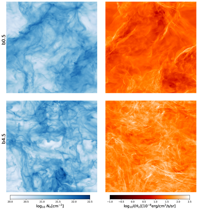
1 Introduction
The abundance of CH+ in diffuse interstellar clouds has been a challenge to explain since it was first identified (Douglas & Herzberg, 1941). The observed column densities (, Lambert & Danks, 1986a) are puzzling due to the multiple efficient destruction mechanisms for CH+: reactions with H, , , and dissociation by ultraviolet radiation. In addition, the reaction
| (1) |
is strongly endothermic and only proceeds appreciably for temperatures , significantly higher than the temperatures characteristic of these clouds. As a result, steady state models fail to produce CH+ in sufficient quantities, predicting column densities at least two orders magnitude below observed values (van Dishoeck & Black, 1986).
Proposed solutions to this problem rely on ways to heat some fraction of the gas, even transiently, to . Elitzur & Watson (1978) proposed that shock waves in diffuse molecular clouds could account for the CH+ production, and two-fluid MHD shock models were subsequently used to model CH+ formation (Flower et al., 1985; Draine & Katz, 1986a, b; Draine, 1986b). Other solutions have also been proposed, including diffuse gas undergoing strong photoelectric heating (White, 1984), dense photon-dominated regions (PDRs) (Duley et al., 1992; Sternberg & Dalgarno, 1995), and heating in boundary layers at cloud surfaces (Duley et al., 1992).
As diffuse interstellar clouds are supersonically turbulent, intermittent shock heating is one possible way to heat enough of the gas to these temperatures. On the basis of laboratory experiments of turbulent flows, Falgarone & Puget (1995) suggested that intermittent dissipation of turbulence could heat diffuse molecular clouds to these temperatures. Pan & Padoan (2009) found that, in compressible MHD turbulence simulations, a few percent of the gas by mass could be heated to in such diffuse molecular clouds, and thus produce the observed amounts of CH+. These findings may also help to explain observed levels of rotational line emission (e.g. Ingalls et al., 2011) as well. High- states of can only be effectively populated in relatively hot gas or through ultraviolet pumping. It is thus not surprising that CH+ column density and rotationally-excited are correlated (Frisch & Jura, 1980; Lambert & Danks, 1986a).
Drift between ionic and neutral species in MHD shocks has been proposed as a way to help overcome the energy barrier in reaction (1) (Draine, 1980; Flower et al., 1985). Myers et al. (2015, hereafter MML15) analyzed MHD turbulence simulations with an isothermal equation of state for the purpose of addressing the CH+ abundance and found that the contribution to the reaction rate from ion-neutral drift was the dominant effect responsible for generating CH+.
In disagreement with the results of MML15 are those of Valdivia et al. (2017, hereafter V17). V17 ran a two-phase, colliding flow MHD simulation and found that CH+ was not primarily produced by high ion-neutral drift velocities in their simulations. Their simulations also under-produced CH+ relative to observations, for reasons that they discuss. For one, it seems that the ion-neutral drift velocity distribution is not converged, and these velocities increase in magnitude at higher resolution. Second, due to the nature of colliding flow simulations that inject a single, warm phase of ISM into the box, they likely underestimate the fraction in low density regions. As well, highly excited may help to overcome the high reaction barrier present in reaction 1.
Our approach bears more similarity to that of MML15. Like MML15, we have run ideal MHD turbulence simulations to understand the abundance of CH+. We use the same abundances of H, , , C, and O, the same mean density, and the same box size to make our simulations as directly comparable to theirs as possible. Two of our simulations use a low initial magnetic field strength (0.5 G), and two use a high magnetic field strength (4.5 G). Two are run with an isothermal equation of state as in MML15, and two are run with an adiabatic () equation of state with heating and cooling processes included throughout the simulation. For all of our simulations, we also estimate the ambipolar diffusion heating in each cell with a post-processing scheme described in section 3.3. This effect is separate from the streaming-induced enhancement of the reaction rate, and similarly important. In our simulations, the ambipolar diffusion heating rate can become the dominant heating term in the low density regions where MML15 determined the majority of CH+ is produced. We present maps of total column density and rotational line intensities for those simulations that include heating and cooling processes throughout in Fig. 1.
Because turbulence leads to disorder in the magnetic field, we check to see whether the proposed levels of MHD turbulence are consistent with observations of polarized emission from aligned dust grains (Planck Collaboration et al., 2015c, 2018).
In section 2 we review our model, the effects of ambipolar diffusion, and the relevant heating processes. In section 4, we detail our (new) calculation for the cooling function and an accurate fit to it for computational ease (see also App. B), as well as describe the C+ and O line cooling that we use. In section 4.2, we discuss details of line emission. Then, in section 5 we describe the chemistry that goes into producing CH+. We present our results for the temperature and drift velocity in our simulations, the CH+ abundance, the velocity distributions of CH+ molecules, rotational line emission, and the polarization of dust emission in section 6. Finally, we discuss our results in section 7 and provide a summary of our findings in section 8. A summary of our simulation parameters and results can be found in tables 1 and 2, respectively.
2 Fluid dynamics
As described in Sec. 1, our simulations are designed to study the formation of the CH+ molecule and emission from rotational transitions in turbulent molecular clouds.
To investigate the importance of magnetic field strength, and to compare different treatments of the fluid dynamics, we have run a number of simulations. In Appendix A, we explore the numerical convergence of our results using resolutions ranging from through . In the body of this paper however, we will focus on simulations run at a resolution of .
For each magnetic field strength, we calculate the fluid motions assuming ideal MHD and explicit heating and cooling. We also carry out simulations using ideal MHD and an isothermal equation of state, to evaluate the effects of heating and cooling on the fluid motions. We post-process these isothermal simulations following a procedure similar to that given in MML15 (see Sec. 3). Our post-processing of the isothermal simulations differs from MML15 in that we use a new cooling function (Eq. 17), and we attempt to estimate the effects of ambipolar diffusion heating on the system as described in the coming sections.
2.1 Models & Scaling
Intermittent dissipation events in molecular clouds arise from the supersonic MHD turbulence that pervades them. To model these clouds, we use the results of four 5123 driven MHD turbulence simulations run with the astrophysical MHD code Athena++.111https://github.com/PrincetonUniversity/athena-public-version These simulations utilize periodic boundary conditions and a cubic domain. They are driven solenoidally between wavenumbers with a power spectrum , where pc is the length of a side of the simulation volume. The driving follows the Ornstein-Uhlenbeck process (Lynn et al., 2012), smoothly evolving the driving with a correlation time of about 1/10 of a dynamical time. We use the Harten-Lax-van Leer-Discontinuities (HLLD) Riemann solver together with a second order Piecewise-Linear-Mesh (PLM) primitive reconstruction with a second order van Leer time integrator. As magnetic fields and their effects in molecular clouds may vary, we use two initial field strengths to compare to one another: 0.5 G and 4.5 G.
Simulations begin with a uniform medium and uniform magnetic field , and are then driven until the velocity dispersion and the root-mean-square magnetic field strength saturate. We adjust the driving so that the saturated value of is close to the observed size-linewidth relation:
| (2) |
where we have let the cloud’s radius pc. The driving power necessary to reach this will vary depending on field strength and equation of state. The values we have adopted for the size-linewidth relation are from Solomon et al. (1987).
The parameters we use are shown in Table 1. Many of these are chosen to reflect values from MML15. We define the plasma as the ratio of the volume-averaged thermal pressure to the volume averaged magnetic pressure. The Mach number is the mass-weighted root-mean-square (rms) velocity divided by the mass-weighted sound speed, and the Alfvén Mach number is the mass-weighted rms velocity divided by the volume averaged Alfvén speed. These definitions are chosen so that the Mach number and Alfvén Mach number are simply related to the ratio of kinetic energy to thermal energy and kinetic energy to magnetic energy, respectively. Like MML15, we adopt a constant composition and assume all of our ions are C+.
| 0.68 | |
|---|---|
| 0.16 | |
| 0.1 | |
| 1.49 | |
| 30 cm-3 | |
| = | g/cm-3 |
| cm-2 |
We neglect gravity. The total mass in our volume is about 8300 M⊙, giving an overall virial parameter , rendering self-gravity negligible. We may also compare the effects of gravity to magnetic fields through the mass-to-flux ratio relative to critical
| (3) |
For our simulations ranges from about 0.7 to 1.9, so these simulations range from somewhat magnetically sub-critical to somewhat super-critical.
We explicitly follow internal energy in our simulations and changes therein due to heating (from cosmic rays and photoelectric emission from dust grains) and cooling (due to C+, O, and line emission). The cooling is not scale-free, introducing a particular length, time, and temperature. When using this cooling function as an explicit source term in a simulation, we are thus given less freedom than when post-processing isothermal simulations.
2.2 Ambipolar Diffusion
| name | |||||||||||||
|---|---|---|---|---|---|---|---|---|---|---|---|---|---|
| units | G | G | G | G | None | None | km/s | None | erg cm-3 s-1 | [cm-2] | erg/s/cm2/sr | None | None |
| b0.5 | 0.5 | 2.4 | 2.5 | 4.3 | 24 | 0.51 | 4.3 | 2.9 | 7.4 | 12.2 | 20.8 | 0.22 | 0.22 |
| b0.5-iso | 0.5 | 2.0 | 2.4 | 3.7 | 24 | 0.68 | 4.0 | 3.1 | 6.7 | 12.3 | 20.4 | 0.18 | 0.21 |
| b4.5 | 4.5 | 6.1 | 5.1 | 9.5 | 0.38 | 0.10 | 3.9 | 1.2 | 10.0 | 13.2 | 45.9 | 0.27 | 0.30 |
| b4.5-iso | 4.5 | 5.8 | 4.4 | 8.6 | 0.38 | 0.13 | 4.2 | 1.4 | 6.7 | 13.1 | 47.8 | 0.24 | 0.29 |
The effects of ambipolar diffusion in the CNM have been treated in three separate ways in MHD turbulence simulations. The first is to treat ions and neutrals as separate fluids that interact through a drag force with frictional heating (Draine, 1986a; Li et al., 2008). This is the most true-to-life of the three methods, but is numerically challenging on the length scales we are interested in, and currently beyond computational reach.
The second approach is a modified MHD treatment that neglects the inertia of the ions and treats ambipolar diffusion as an extra diffusive term in the magnetic induction equation (Mac Low et al., 1995). It assumes that ions stream relative to the neutrals at an instantaneous velocity given by
| (4) |
where is the magnetic field, is the ion-neutral coupling constant, is the density of neutral species, and is the density of ions. Here is the momentum transfer rate coefficient, and and are the ion and neutral mass per particle. The magnetic field would be evolved according to
| (5) |
This second approach is prohibitively expensive for this problem as well. For the 20 pc scales we are interested in, the ambipolar diffusion length is very small in the highest density regions. As a result, to resolve the effects of ambipolar diffusion in these regions would require extremely high resolution. Further, the time-step required for numerical stability in this method scales as , the spatial resolution squared. The combination of these factors make this approach infeasible for our problem.
The third approach is to assume that ideal MHD can be used to evolve the density, fluid velocity, and magnetic field. An additional approximation often made is that the ion-neutral drift velocity can also be approximated by Eq. 4 with taken to be the field computed assuming ideal MHD. This approach relies on estimating the effects of ambipolar diffusion in post-processing, rather than self-consistently in real time. Our approach is most similar to this third approach, with some important modifications.
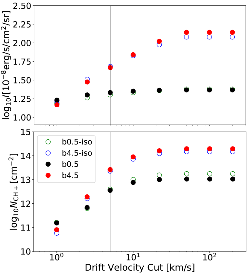
Naively assuming that Eq. 4 accurately reflects the ion-neutral drift velocities everywhere in a simulation volume leads to several issues. The volume-averaged heating rate calculated with Eq. 4 can easily exceed the volume-averaged driving power, which is unphysical. The heating power per mass may be very large in low density regions, where the drift velocities given by Eq. 4 can become very large (see Figure 17). A conservative way of dealing with these high drift velocities and heating rates is to exclude from our analysis regions where the drift velocity exceeds some chosen threshold. The exact value of this cut will have an effect on our results. Figure 2 examines the effect that this cut has on our results.
3 Heating processes
As we have simulations with both an isothermal equation of state and a non-isothermal equation of state, we must incorporate heating in two separate ways.
The first (used for the isothermal equation of state) is to determine the temperature in each cell after the simulation is completed assuming a balance between all cooling and heating processes. Formally, a temperature is computed in each cell where
| (6) |
where (described in Sec. 4) is the total cooling in that cell and is the total heating including cosmic ray and photoelectric heating and an estimate for the viscous heating (see Secs. 3.1 and 3.2). Ambipolar diffusion heating is treated differently, and described in Sec. 3.3.
The second is to use the explicit integration scheme implemented in the MHD code Athena++ to include the extra heating and cooling terms (described in Secs. 3.1, 4) dynamically throughout the time domain of the simulation. This method implicitly handles both viscous and shock heating, and has the advantage of allowing for the possibility of adiabatic heating and cooling. However, this can also make the method prohibitively expensive. Occasionally, rarefactions in already cold (dense) gas will adiabatically cool gas well below the equilibrium temperature (which may be as cold as 10 K in the case of gas with ). For heating that is proportional to density (as in cosmic ray and photoelectric heating, described below in Sec. 3.1, 3.2), such dense gas may have a large heating rate, but a small internal energy, leading to a restrictive thermal time step. In this case, we impose a limit on how cold the gas can get, and suppose that it cannot cool below 2.7 K. While this means we effectively inject energy into these few extremely cold regions, the amount is small compared to the other heating terms, and so should have a negligible impact on the global dynamics and chemistry of the simulation.
3.1 Cosmic ray & photoelectric heating
Cosmic ray ionizations and the photoelectric effect on dust grains both serve to heat the cold neutral medium.
The heating due to cosmic ray ionizations is a combination of the cosmic ray ionization rate per hydrogen nucleus , the heat per ionization , and the density . We take from Indriolo & McCall (2012) and eV from Glassgold et al. (2012).
Our chosen and are identical to those chosen in MML15 so that our results are as directly comparable as possible. The cosmic ray heating is thus
| (7) |
The dust photoelectric heating rate can be written (Wolfire et al., 2003)
| (8) |
with being the heating efficiency and the FUV intensity in the units of Habing (1968). For (Mathis et al., 1983), and typical parameters (), , and thus
| (9) |
four times larger than .
3.2 Viscous heating
While viscous heating is handled implicitly in Athena++ when we use a non-isothermal equation of state, for simulations with an isothermal equation of state we determine the temperature using a post-processing scheme similar to that in Pan & Padoan (2009) and MML15. To estimate the viscous heating in each cell of the simulation, we first compute the rate of shear tensor :
| (10) |
where denotes the transpose, and is the euclidean metric tensor. The gradients here are determined using a cell-centered finite difference method, and so should be second order accurate in the spatial resolution. Given , the viscous heating in a cell is
| (11) |
The kinematic viscosity here is not of physical origin; it’s a numerical viscosity. Similarly to MML15, we estimate its value by allowing to be a normalization such that the total viscous heating in the simulation is equal to the input driving power; in other words, we assume that all the input driving power goes into viscous heating.
3.3 Ambipolar diffusion heating
We do not include ambipolar diffusion in the dynamics of our simulation. However, in low density regions, ambipolar diffusion can become an important heating mechanism. In order to best estimate what the thermal effects of ambipolar diffusion would be in our simulations, we begin with the temperature either from the code directly (as is the case with simulations b0.5 and b4.5), or post-processed following a procedure similar to that given in MML15 (done for the isothermal simulations b0.5-iso and b4.5-iso). Given these temperatures , we compute a new temperature by solving the following equation in each cell of the simulation:
| (12) |
where is the heating rate per volume due to ion-neutral friction. This may be expressed as
| (13) |
where is the ion-neutral coupling coefficient (taken to be between C+ ions and , identical to that in Eq. 4), and is the ion-neutral drift velocity (see Eq. 4). This assumes instantaneous balance between heating and cooling, which will only be approximately true. It is important to note, however, that this does not throw out our hard-earned dynamical heating, as the new temperature is bounded by the old temperature from below, or
| (14) |
4 Cooling processes
4.1 Fine Structure Lines
In the cold neutral medium, the main avenues for cooling we expect are due to the species , O, and . For and O, we use
| (15) | ||||
| (16) |
These values have been scaled from their original values in Wolfire et al. (2003) to reflect our C and O abundances.
4.2 Line Emission
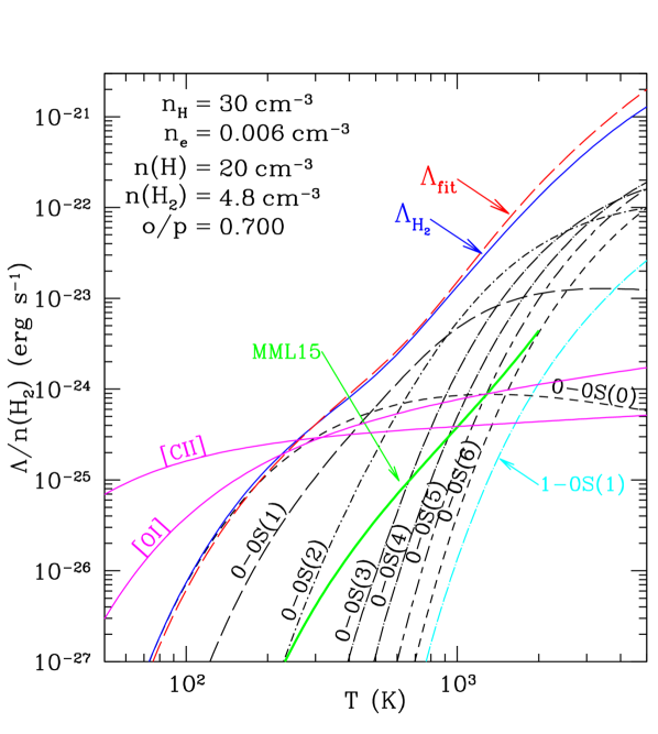
The rotation-vibration lines of can be important cooling channels. We employ a new cooling function that is easy to evaluate, but which provides a good approximation to detailed calculations of excitation over a wide range of densities, temperatures, and molecular fractions. Our new cooling function is based on up-to-date collisional rate coefficients, as described in Appendix B. Figure 3 shows the cooling rate for and molecular fraction that MML15 took to be a representative example for gas in a turbulent molecular cloud. We fix the ortho/para ratio at the value adopted by MML15. The cooling for this case is shown in Figure 3.
The total cooling is shown (blue solid curve) for . Also shown are the powers in selected emission lines. For the cooling is dominated by 4 rotational lines: , , , and . At temperatures , rotational lines from become important, and for the vibrational transitions (e.g., ) begin to make a significant contribution to the total cooling.
In Figure 3 we also show the cooling power (per molecule) in the [CII]158 and [OI]63 fine structure lines. We see that for the conditions considered in Figure 3, the fine structure lines dominate the cooling for , but for the cooling is dominated by .
Figure 3 also shows the cooling function from MML15, for . The MML15 cooling function is smaller than the present by a factor .
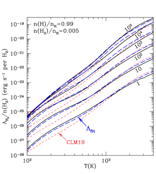
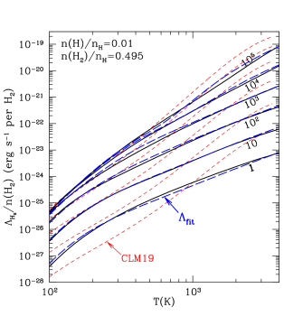
The resulting cooling power per , , is shown in Figure 4 for selected densities , for gas that is predominantly atomic (Fig. 4a) and predominantly (Fig. 4b). The atomic and molecular cases differ because the rate coefficients for collisional excitation of by and by can in some cases differ by large factors. For example, at the cooling power per is times larger in atomic than in molecular gas with the same .
At densities , is approximately linear in , with almost all collisional excitations followed by radiative decay. At high densities the level populations approach LTE, and becomes independent of density.
For computational purposes, it is useful to have an analytic function that provides an acceptable approximation to the “exact” cooling function for K:
| (17) | |||||
| (18) | |||||
| (19) | |||||
| (20) | |||||
| (21) |
The coefficients multiplying in Eq.(18-21) reflect the collisional rate coefficients for excitation by relative to excitation by H and He. We see that Eq. (17) provides a fairly good fit to over a wide range of temperatures and densities, for both atomic gas (Fig. 4a) and molecular gas (Fig. 4b).
Coppola et al. (2019) (hereafter CLM19) provide a fitting function for cooling over the – temperature range. Figure 4 compares the CLM19 fitting function to our calculated cooling rates in predominantly atomic gas: the CLM19 fitting function tends to underestimate our computed cooling rates by factors of for .
Both CLM19 and the present study use H-H2 collision cross sections from Lique (2015). The difference in the cooling appears to be due to differences in adopted rates for collisional excitation by He: Coppola et al. (2019) used quasi-classical trajectory cross sections from Celiberto et al. (2017) whereas we use quantum-mechanical results from Le Bourlot et al. (1999), which are believed to be more accurate at low energies.
For molecular gas, the CLM19 fitting function underestimates the cooling rate by a factor of for temperatures , and overestimates it by a similar factor for . Both the present study and CLM19 assume ortho-para equilibration, resulting in a low ortho-para ratio at the lower temperatures.
5 CH+ Chemistry
When ions are streaming through the neutrals, the rate for the endothermic reaction (1) is affected by the nonthermal distribution of ion-neutral impact speeds. Following Flower et al. (1985) we employ a rate coefficient which is a function of an effective temperature
| (22) |
where is the reduced mass of C+ and and is the Boltzmann constant. This applies when (Pineau des Forets et al., 1986). When , we instead have that the reaction rate is a function of
| (23) |
As with MML15, we assume instantaneous balance between formation and destruction of CH+. The rate coefficients for each of the various creation and destruction mechanisms are
| (24) | ||||||
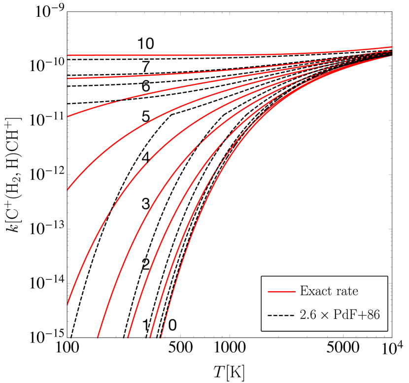
is an approximate form given by Pineau des Forets et al. (1986), but increased by a factor 2.6 to better match the exact rate shown in Fig. 5. In Fig. 5, we compare the Pineau des Forets et al. (1986) approximation against The "exact" rate in Fig. 5 is calculated following Draine & Katz (1986a) for various using the cross section for the , state of (Gerlich et al., 1987; Zanchet et al., 2013). , and are those from the Meudon PDR code222https://ism.obspm.fr/?page_id=33. is from Barinovs & van Hemert (2006), while is from Chakrabarti et al. (2018). Balancing formation with destruction gives
| (25) |
It is clear from this expression that the CH+ abundance is most sensitive to the abundances of C+ and . Solving for the abundance as a function of time when perturbed from equilibrium, one finds that the chemical relaxation time is on the order of 250 years, much shorter than all other time scales in our simulation, so the assumption of equilibrium chemistry is a good one.
6 Results
6.1 Temperature & ion-neutral drift
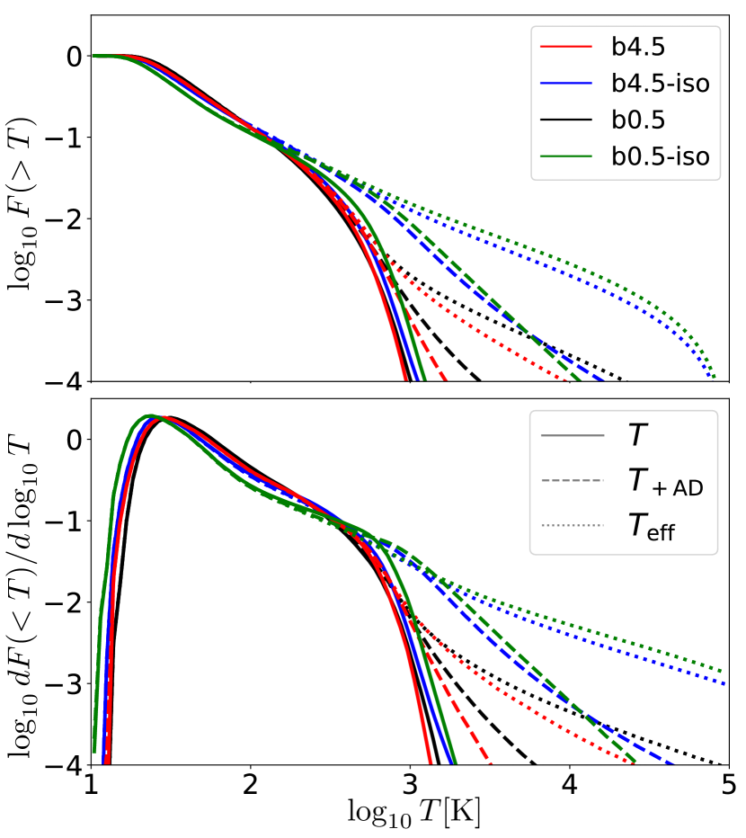
The chemistry we are primarily interested in takes place in gas with temperatures K. Fig. 6 shows that in our simulations, the mass-fraction of the gas with either or is , just as Falgarone & Puget (1995) and Pan & Padoan (2009) suggested was necessary to produce the observed column densities of CH+. If the temperature becomes too high, (K) molecular hydrogen will be dissociated. We also suppose that CH+ production will cease if the ion-neutral streaming velocity exceeds 22 km/s, where the center-of-mass energy is sufficient to dissociate via .
With ideal MHD, we find the drift velocities given by Eq. 4 can sometimes become very large in low density regions, sometimes reaching values as large as 100 km/s in very low density regions. In nature, were drift velocities this high produced, they would (1) self-limit by decreasing the magnetic field strength directly through diffusion, and (2) create high ambipolar diffusion heating rates that would drive up the temperature and thus ionization of the gas, leading to stronger ion-neutral coupling and a drop in the drift speed. We thus suspect that in the cold neutral medium, drift velocities do not routinely reach these high values km/s. For these reasons, we choose to simply ignore CH+ production in regions in our simulation where the drift velocity exceeds 5 km/s. We explore the effect of varying this cutoff velocity in Fig. 2.
6.2 CH+ abundance
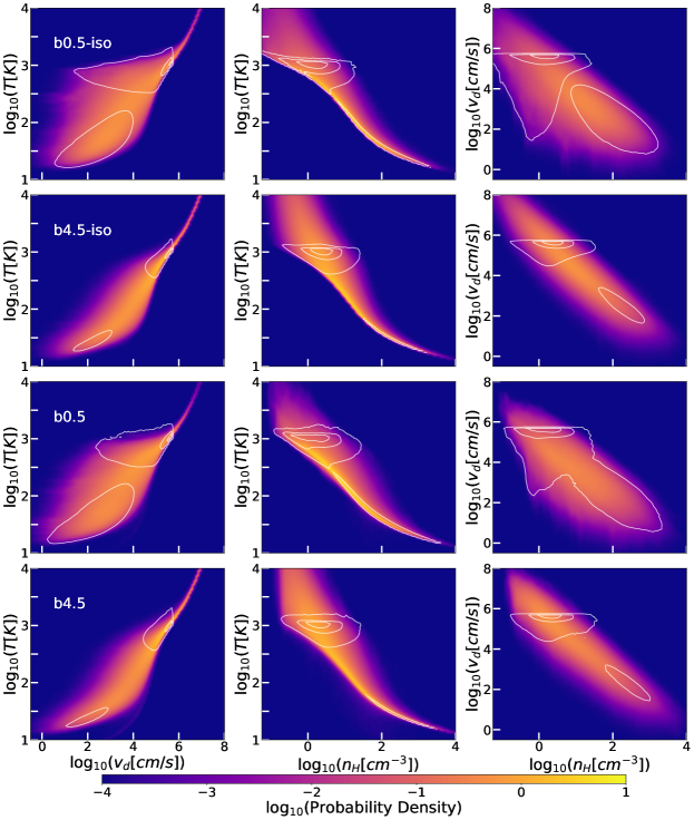
With the CH+ formation rate depending on the effective temperature , we expect the CH+ abundance to be biased towards both high and high ion-neutral drift velocity regions. These regions happen to mostly coincide. In Fig. 7, we show joint histograms of vs. drift velocity, vs. density, and drift velocity vs. density for each of our four simulations. The white contours in Fig. 7 represent where 99%, 90% and 50% of the CH+ exists on each plot. These contours demonstrate that in all of our simulations, CH+ is produced in low density ( cm-3), high drift velocity ( km/s), hot regions ( K).
However, these two modes for creating CH+ are not equal in efficacy. For both the high field strength simulations (b4.5 and b4.5-iso) and the low field strength simulations (b0.5 and b0.5-iso) it seems that high drift velocity regions are responsible for the vast majority of CH+ production. Fig. 2 shows that when we exclude regions with , as we decrease , the CH+ abundance in the simulations is attenuated beginning at about km/s in all simulations. As we reduce down to 1 km/s nearly all of the CH+ vanishes, with our abundances falling to between and cm-2.
As another way to estimate the effect of ion-neutral drift on CH+, we may use the ordinary temperature instead of or in computing the CH+ abundance using Eq. 25. Doing so, we find median CH+ column densities that are lower than those listed in Table 2 by a factor of between 16 and 50 (depending on the simulation), far below those observed in Weselak et al. (2008b). This suggests that ion-neutral drift is critical for CH+ formation.
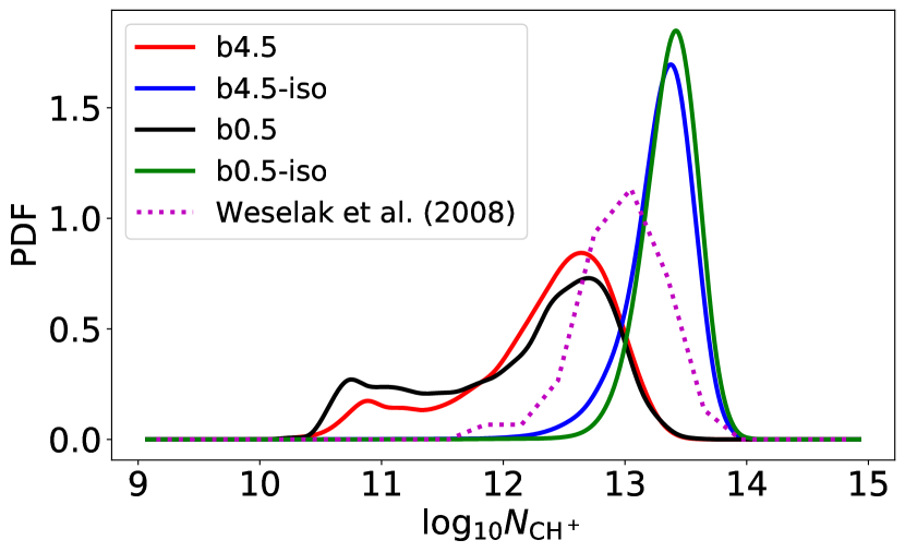
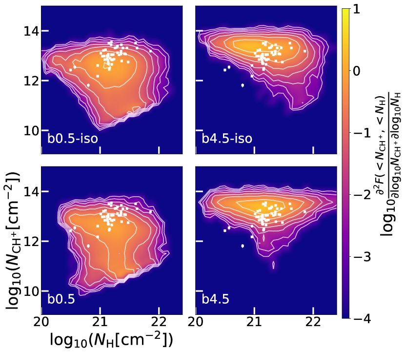
In Figs. 8 and 9, we compare the results of our model to Weselak et al. (2008b)’s data. Fig. 8 shows reasonable agreement between the Weselak et al. (2008a) data and our simulations b4.5 and b4.5-iso, though there may be a larger tail to low CH+ column density in the observations than in our simulation data. In Fig. 9 we do not find the same correlation between column density of H nuclei and CH+ in our simulations that seems to be present in the Weselak et al. (2008b) sample.
Our simulations assume a constant fraction, – we do not follow formation and destruction of , which would require treating the radiative transfer of the far-UV photons responsible for photodissociation of . Thus the low sightlines in our simulations support CH+ formation via reaction (1). In the real ISM, however, sightlines with tend to have low fractions, because photodissociation is insufficiently suppressed by self-shielding (Draine & Bertoldi, 1996) – this accounts for the absence of CH+ detections for in Weselak et al. (2008b).
Our simulations were limited to a single molecular region, whereas observations may sample molecular regions that are both smaller and larger. However, our simulated simulations are quite clumpy, so that sightlines sample column densities ranging from to cm-2 (see Figs. 1, 9), similar to the range of values in the Weselak et al. (2008a) sample.
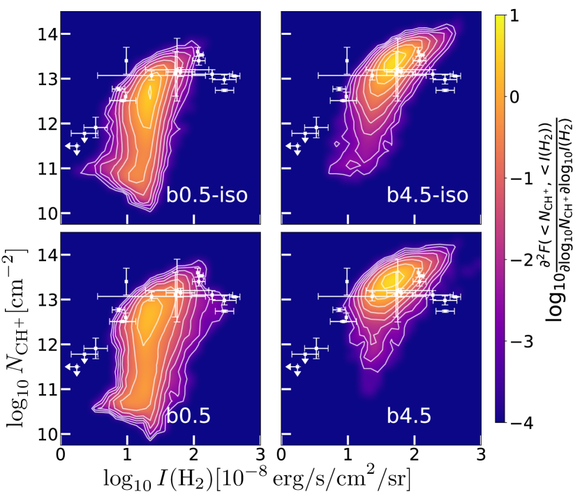
In this study, we define as the intensity of emission from the first three rotational lines 0-0 , , and . How it is computed from the simulations and observational data is specified in section 6.4. Comparing to , Fig. 10 shows a strong correlation between these quantities, in particular where column densities of CH+ are high or where is high. This is in line with the observed correlation of rotationally-excited with (Lambert & Danks, 1986b; Frisch & Jura, 1980; Spitzer et al., 1974).
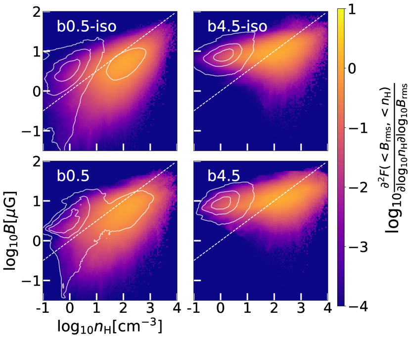
Figure 11 shows the joint probability density function of magnetic field strength versus number density of hydrogen nuclei, with contours containing 50%, 90%, and 99.9% of the CH+ in our simulation. As CH+ appears to cluster around densities in our simulations, we may consider the CH+ column density to be a probe of the heating processes in the lowest density molecular regions.
6.3 Synthetic CH+ velocity distributions
We construct synthetic line-of-sight (1D) particle velocity distributions for and CH+ for qualitative comparison with observations (e.g., Pan et al., 2004). In each cell of a simulation, we have the neutral fluid velocity and the ion-neutral drift velocity (calculated as in Eq. 4). The fluid velocity of the ions in that cell is
| (26) |
We assume Maxwellian velocity distributions, centered on for neutrals, and for ions. In addition, below the grid scale of the simulation, there will be some microturbulent contribution to the velocity dispersions of both the ionic and neutral species. If the power spectrum for each simulation were purely Kolmogorov, this microturbulent contribution would be km/s, and this is the value we assume. The total width of the velocity distribution for a species in a cell is therefore,
| (27) |
where is the Boltzmann constant, is the kinetic temperature of species in cell , and is the mass of species .
The velocity profile of a species at a velocity is
| (28) |
where is the number density of species in cell , and is the physical size of a cell.
Eq. 27 has a species specific temperature, for the possibility of ions being out of thermal equilibrium with the neutral species. Ion-neutral scattering will heat the ions to a temperature where heat transfer to and from the ions (Draine, 1986a) vanishes,
| (29) |
where is the mean mass of the neutrals (see Tab. 1), and is the Boltzmann constant.
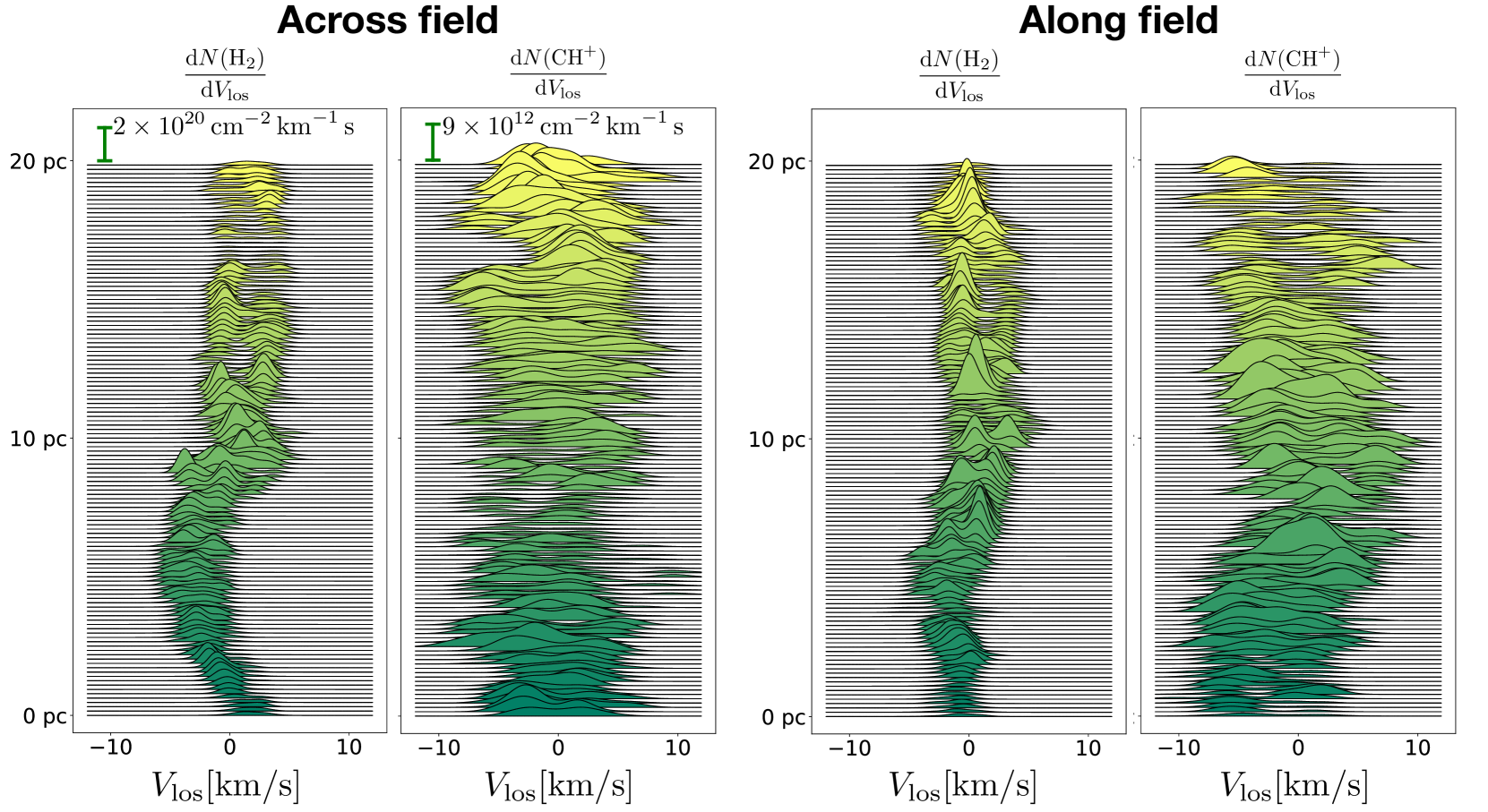
Constructing these velocity profiles for CH+ and in our simulations (Fig. 12), we see that the CH+ is consistently broader than the velocity profiles. As well, we often see multiple components of CH+, sometimes separated by 10 km/s. For neutral line profiles, while we do see multiple components, as km/s, we do not see component separations of more than a few km/s.
6.4 rotational line emission, 0-0
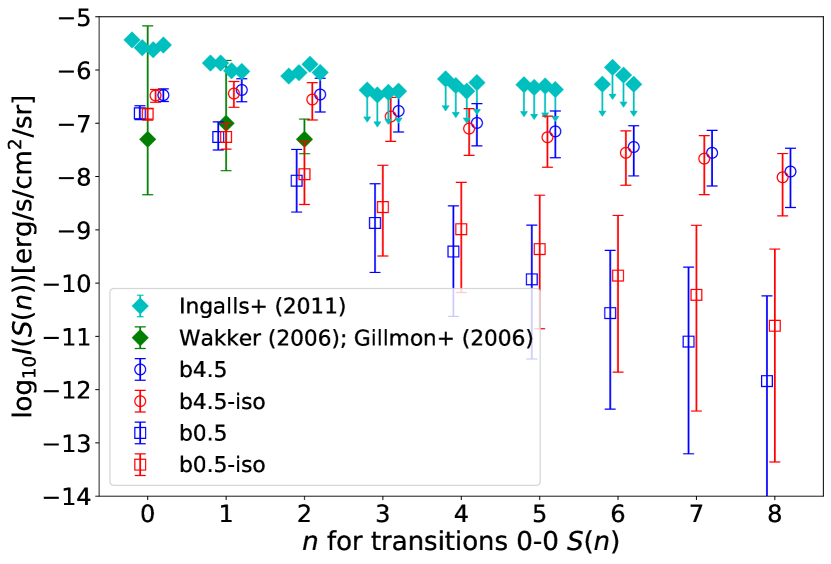
Figure 13 shows the intensity of rotational emission lines 0-0 from through in each of our simulations, computed using the temperature . As is the case with all of our analysis in this paper, we exclude regions where the ion-neutral drift velocity exceeds 5 km/s. The higher field strength simulations (b4.5 and b4.5-iso) exhibit a notably higher level of emission compared to the low field strength simulations (b0.5 and b0.5-iso), especially at higher . Even with the obvious enhancement of the line intensities from the ambipolar diffusion heating, we still do not reach the line intensities seen by Ingalls et al. (2011) at four positions on the high-latitude translucent cloud Dcld 300.2-16.9. Other excitation mechanisms appear to be necessary to explain the Ingalls et al. (2011) intensities. However, our simulations do largely agree with other data. In Fig. 13, we also plot median values of the intensity of 0-0 , , and for AGN sightlines from Wakker (2006) and Gillmon et al. (2006) towards AGN. As well, the data in Fig. 10 from Lambert & Danks (1986b), Spitzer et al. (1974), and Frisch & Jura (1980) show good agreement with both of our simulations.
As mentioned in section 6.2, one point of comparison between observations and our simulations we use is the sum of the intensities of the first three rotational lines 0-0 S(0), 0-0 S(1), and 0-0 S(2). We call this quantity . These first three lines contain most of the emission from , and so reflect dissipation into .
Observations of plotted in figure 10 are computed using known transition rates from the , levels of into the , levels, respectively (Wolniewicz et al., 1998) together with reported -level column densities.
For all but one of the points, errors are computed from the errors on the column densities in the source literature. For the one point that is not, the column density for was unavailable. To compute upper and lower bounds on the point, we thus see what the greatest ratio of is across the observations to compute an upper bound on , and similarly to compute a lower bound. We take the (logarithmic) midpoint between the upper and lower bounds to be our value for and compute from this.
All of our simulations exhibit a correlation between and , as is shown in Fig. 10. In our high field strength simulations, b4.5 and b4.5-iso, there is a relatively strong correlation between and , with only dex of scatter in for any given . However, at low field strengths, as in b0.5 and b0.5-iso, this correlation is only apparent at higher values of , with the correlation disappearing when . As the velocity dispersions are similar across both field strengths, the explanation for the difference between the joint vs. histograms must lie in their differing ion-neutral drift velocity distributions.
In Fig. 10, we also plot six lines of sight towards various stars, with CH+ column densities from Lambert & Danks (1986b) and computed using column densities of the , states of published in Spitzer et al. (1974) and Frisch & Jura (1980). These observations agree much better with our simulation data than those from Ingalls et al. (2011). It may be that the Ingalls et al. (2011) cloud is in some way atypical compared to these other simulations.
The higher ion-neutral drift velocities present in our simulations b4.5 and b4.5-iso produce higher values of compared to our low field strength simulations. Higher values of mean higher values of . Higher values of also mean higher values of CH+, but as we stated, the drift velocity dependent component of is much more important to CH+ than .
6.5 Polarization and the Stokes parameters, and
To compute the polarization of starlight and thermal emission due to dust grains along a particular line of sight, we compute dimensionless quantities , , and
| (30) | |||||
| (31) | |||||
| (32) |
where denotes the component of the magnetic field along direction , and subscripts on each of the , , and denote the axis along which we integrate. The mean field direction is along , so the above represent sight-lines perpendicular to the mean field. When computing these parameters along the mean field direction, we simply take .
Starlight from a star behind the cloud would have fractional Stokes parameters
| (33) |
and fractional polarization
| (34) |
where is a starlight polarization cross section, and measures the degree of alignment of dust grains with the local magnetic field (see Appendix C).
For thermal emission, the Stokes parameters and , and the polarized intensity , are directly related to , , and , but must also be averaged over a beam: (see Appendix C):
| (35) | |||||
| (36) |
where denotes an average over a beam with beam size parameter , and is the black-body spectrum of a dust grain at temperature . The fractional polarization is (see Appendix C)
| (37) |
Planck Collaboration et al. (2018) find that and are highly correlated, with Pearson correlation coefficient 0.92 for a beam with FWHM=40 arcmin. Planck Collaboration et al. (2018) also find that the ratio changes minimally when the beam size is varied from 20 arcmin to 80 arcmin.
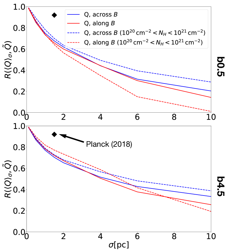
Fig. 14 shows the Pearson correlation coefficient between the beam-averaged and the line-of-sight polarization parameter , as a function of gaussian beamsize
| (38) |
for our b4.5 simulation. The correlation is shown for random sightlines along the mean field , and across . We see that for this simulation, drops below for . This contrasts with observations showing for (for a typical distance to the emitting dust).
In order to study the coherence of the polarization in our simulations, we examine at the polarization angle dispersion function defined by
| (39) |
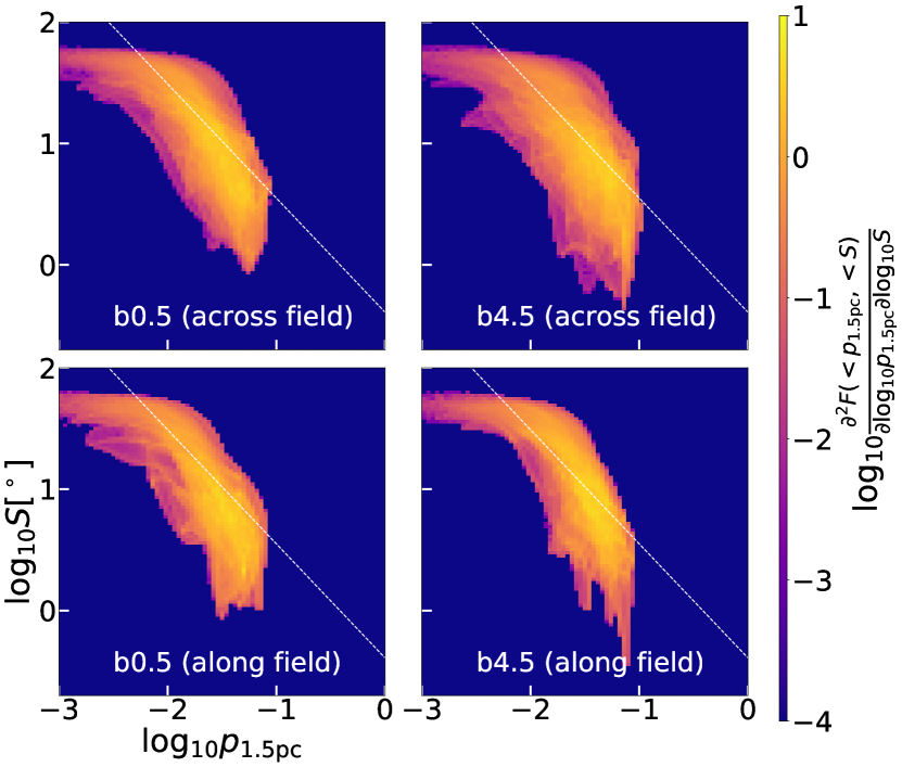
where the sum runs over all lines of sight in an annulus of radius and width 0.75 pc centered around a position , is the polarization angle at , and is an offset that puts in the aforementioned annulus (Planck Collaboration et al., 2015a). This corresponds roughly to the parameters that Planck Collaboration et al. (2015a) used for this function given a beam FWHM of 60 arcmin and an annular radius and width of 30 arcmin if we place our simulation at a distance of . For consistency, we also use a gaussian beamsize pc to compute the angles . Fig. 15 shows versus for our simulations b0.5 and b4.5. To compute this quantity, we have assumed that . We choose this value because 0.24 is the best estimate for the highest observed level of polarization in Planck Collaboration et al. (2018). Choosing this value for ensures that our computed polarizations are always .
This function has the property that completely random orientations of the polarization yield , explaining the asymptotic behavior at low in Fig. 15. Planck Collaboration et al. (2015a, b) found an approximate relationship in both their observational data as well as in a colliding flow MHD simulation. We also find this relationship (shown as a white dashed line in Fig. 15) to approximately hold true for our simulations as well. It is interesting to note that altering the mean field strength/Alfvén Mach number seems to have no effect on this relationship. The relationship also seems unaffected by whether or not we are looking along or across the mean magnetic field direction.
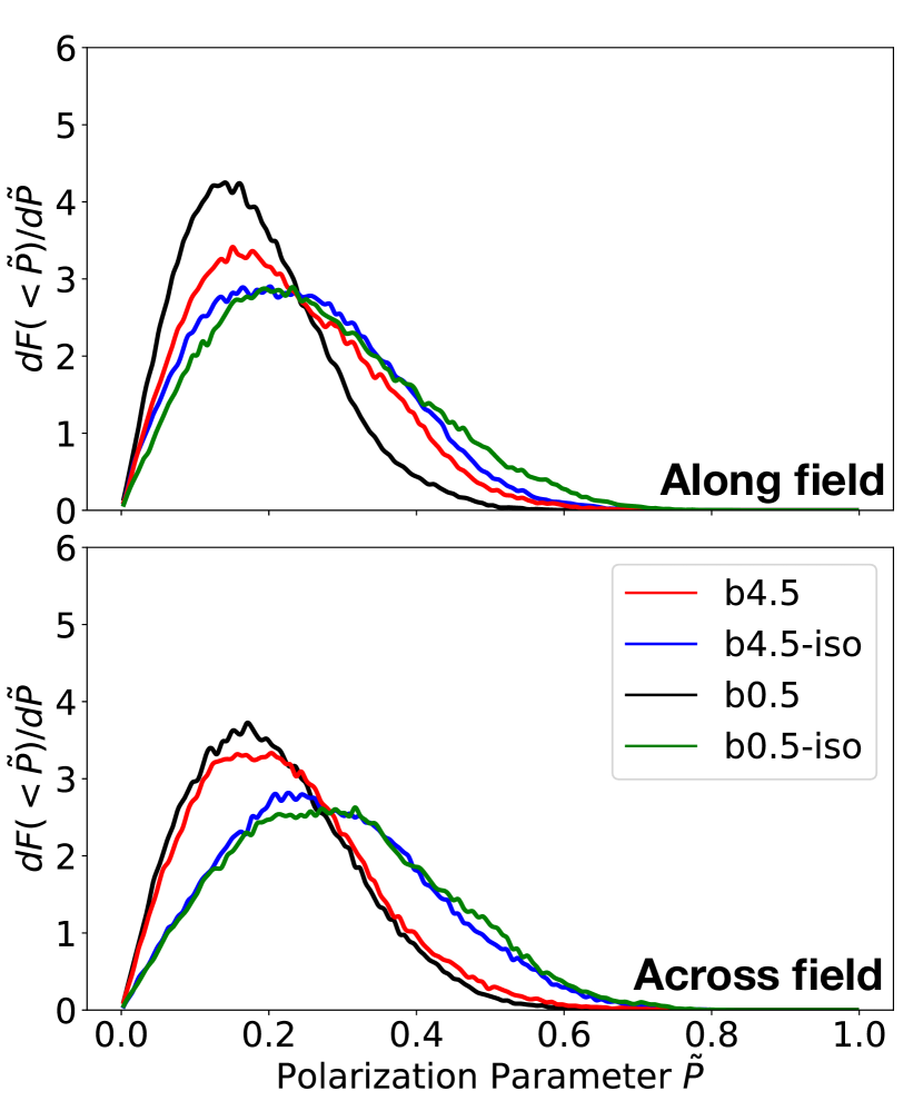
Given that our four simulations differ in one of two ways (either field strength or isothermal/non-isothermal), we may examine the effect that each of those variables has on the polarization. Firstly, does including heating and cooling processes throughout the simulation impact the magnetic field geometry? Fig. 16 shows probability density functions for line-of-sight polarization in each of our simulations for 5122 sight lines, both across and along the mean field.
We see no marked difference between polarization in simulations run with an isothermal () equation of state versus simulations run with and heating (cosmic ray, photoelectric emission from dust grains) and cooling (, C+, and O) processes included. This suggests that, for the purposes of studying polarization, isothermal MHD turbulence is a reasonable approximation, with heating and cooling processes having only a small effect on the PDFs of dust polarization along lines of sight.
As might have been expected, the higher field strength simulations exhibit higher values of (see Fig. 16), with the difference being most apparent when looking across the mean field. This makes intuitive sense, as the higher field strength simulations are only moderately super-Alfvénic, with . The magnetic field in those simulations is thus moderately effective at resisting distortions due to the turbulent motions in the cloud.
When looking down the field, the polarization we see in all simulations will be due only to a random component of the magnetic field. As a result, we do not expect to see polarization levels quite as high looking along the mean field as looking across the field, nor do we expect as large a difference between the polarization levels for different magnetic field strengths. Indeed, this is what we observe in Fig. 16.
7 Discussion
In our simulations, turbulence and the ambipolar diffusion heating that results from it raise the gas temperature in low density regions to beyond , sufficient to produce CH+. High ion-neutral drift velocities (Eq. 4) also enhance the CH+ abundance through increasing the effective reaction temperature (Eq. 22, see also Fig. 6). As ion-neutral drift velocities are highest in low-density regions, the CH+ exists predominantly in regions with . In some fraction of the volume, these drift velocities exceed 5 km/s, and so have an ambipolar diffusion Reynolds number . As ambipolar diffusion is important to the dynamics in those regions but we have not properly included it in the dynamics, we have excluded these regions when calculating CH+ formation and line emission in our models. This is an important caveat of our results, as the details of these regions could be very important to both the CH+ abundance and the rotational line emission (see Fig. 2).
Our simulations include sight-lines where and (see Fig. 9. Such sight-lines are not seen in the data (e.g. Weselak et al., 2008b). Because our simulations do not include formation/destruction of , even low column density regions are assumed to have a relatively high fraction, and thus are able to form CH+ in our simulation. In reality, photodissociation will suppress the fraction in low column density regions, where self-shielding is ineffective. Proper treatment of the variable fraction requires radiative transfer including self-shielding (V17).
The CH+ column densities found in MML15 lie between the results of our lowest (b0.5 and b0.5-iso) and highest (b4.5 and b4.5-iso) magnetic field strength simulations. In this way, our results are consistent with theirs. We find that ambipolar diffusion can become a significant factor contributing to the heating of the volume, and cannot be neglected energetically. MML15 found that the contribution to the CH+ abundance from the ion-neutral drift velocities to be the dominant effect responsible for producing CH+; we corroborate this finding. The fact that CH+ is predominantly produced by the ion-neutral drift velocities in our model as well as in the MML15 model is the reason that our results qualitatively agree despite the large discrepancy in our cooling functions. Both our paper and theirs rely on the same post-processing method to deduce the ion-neutral drift velocities.
As mentioned in section 1, V17’s two-phase, colliding flow results contrast with our findings and those of MML15. V17 found that CH+ was not primarily produced by high ion-neutral drift velocities in their simulation. As well, their simulation under-produced CH+ relative to observations, finding column densities rather than . The reasons for this appear to be three-fold. First, destruction of in low-density regions limits CH+ production by reaction (1). Second, a higher ionization fraction means that ion-neutral drift velocities will be lower, and as we find CH+ is very sensitive to changes in the ion-neutral drift velocity, this can have an enormous impact on the overall CH+ abundance. V17 found overall drift velocities around two orders of magnitude lower than those we find. Third, injecting only warm-phase ISM into the box seems likely to underestimate the fraction in the lower density regions, further decreasing CH+ abundance.
We suspect there are also key differences in the way the problem is set up in our simulations versus those of V17. V17 used a 2.5G guide field aligned with the direction of their flow. We expect this configuration would naturally lead to less tangling of the field in much of the simulation, in particular in the low density regions where CH+ is likely produced. In contrast, we used a stronger 4.5G mean field and drove turbulence isotropically. It is hard to directly compare our results with theirs given the lack of information on their rms magnetic field strength, Alfvén Mach number, and velocity dispersion in the CNM phase. It seems guaranteed that a colliding flow simulation of this type would produce results differing from those of a simulation of driven turbulence. It would be interesting to know how well a simulation of the V17 type compares to observations of polarization with the same metrics we have used. To understand this problem, multiphase simulations with realistic driving analogous to stellar winds and supernovae are needed.
Of course, both colliding flow simulations and driven turbulence are artificial in their own ways, and likely to produce discrepant results. It is clear that the main difference between our results and those of V17 is the ion-neutral drift velocity. It is essential that future work accurately capture this physics, or at least explore its effect realistically. The biphasic nature of their simulation also impacts the drift velocity distribution. It would be informative in future work to do a multiphase study with formation and destruction as in V17, but using higher rms magnetic field strengths and a periodic domain driven at large scales the way we have in our study. Recently, Körtgen (2020) showed that turbulence driving in disc galaxies is neither purely compressive nor purely solenoidal.Future simulations may employ driving of this type instead of purely solenoidal driving as we have done.
Our simulations with produce rotationally-excited at levels approximately consistent with UV absorption measurements of rotationally-excited , and the observed correlation between CH+ and rotationally-excited is also reproduced (see Figs. 10 and 13). However, our models fall short of the strong infrared emission observed from the quiescent translucent cloud DCld 300.2-16.9 (Ingalls et al., 2011). It appears that some additional process is contributing to the excitation in this cloud.
Planck observations of polarized emission from dust provide a strong test of MHD simulations. The fact that the polarization of dust emission in our simulations is so effectively destroyed by averaging over beams a few pc in size (Fig. 14) is puzzling when compared to the Planck Collaboration et al. (2015d) data. Perhaps the mean field should be even stronger than , thus lowering the Alfvén number. Or perhaps ambipolar diffusion (or some other field-smoothing mechanism) acts more strongly than we have assumed in our simulations, in which ambipolar diffusion has not been treated self-consistently.
In the future, two-fluid simulations that include ambipolar diffusion, full radiative transfer, variable ionization fraction, and time-dependent chemistry will be necessary to fully disentangle all of the separate variables and fully understand the problems we have addressed in this paper. It may not be feasible to model all of these things at once in a volume similar in size to what we have studied here (8000 pc3), and realistically, future simulations will likely capture one or several of these effects at once, unless effective sub-grid models can be developed.
8 Summary
We present MHD simulations of diffuse molecular clouds 20 pc in size using two different mean magnetic field strengths (0.5G and 4.5G). All simulations have the same 3D velocity dispersion (within 10%) chosen to remain consistent with the linewidth-size relation for molecular clouds (Solomon et al., 1987). We compare simulations using an isothermal equation of state with non-isothermal simulations including realistic heating and cooling. We calculate cooling over a range of temperatures, densities, and fractions, and provide an accurate fitting function for the cooling. The MHD simulations were post-processed in a way similar to MML15 to calculate CH+ abundances, and excitation and line emission. We compare these results to observations and find that we can explain the CH+ abundance (Figs. 8, 9), and rotational excitation of in many regions (Figs. 10, 13. However, we fall short of explaining the strong rotational line intensities seen from two translucent clouds (Ingalls et al., 2011). The line emission is correlated with the CH+ (Fig. 10).
CH+ appears to be primarily manufactured in low density regions with high ion-neutral drift velocities. These high ion-neutral drift velocities significantly complicate the interpretation of our results because they can become unphysically large. Because of concern about the realism of the high-drift-velocity regions, we calculate CH+ production and line emission only from regions where the drift velocity km/s, corresponding to ambipolar diffusion Reynolds number . We examine the effects of this cutoff on total rotational line emission and CH+ abundance in figure 2.
We also construct synthetic line-of-sight velocity distributions for CH+ and molecules (Fig. 12). The CH+ profiles tend to be broader than the neutral line profiles, especially in simulations with a higher mean magnetic field strength.
We compute the polarization of starlight and thermal emission from dust grains and in our MHD simulations, and compare our results to those of Planck Collaboration et al. (2018). The polarization statistics are largely unaffected by which method was used for the hydrodynamics (including heating and cooling processes vs. using an isothermal equation of state). The polarization does depend on field strength/Alfvén Mach number, with higher field strength (lower Alfvén Mach number) corresponding to higher levels of polarization (Fig. 16).
We examine the effect of averaging the Stokes and over a gaussian beam of varying width and find our simulations to be marginally inconsistent with the findings of Planck Collaboration et al. (2018).
The correlation between beam-averaged polarization of dust thermal emission and polarization of starlight along a sightline is too low in our simulations. We suspect that this is due to our Alfvén Mach number in our simulations () being higher than that in nature (perhaps ) on these scales. We speculate that perhaps field-smoothing by ambipolar diffusion in nature is more effective than in our simulations, which do not treat ambipolar diffusion self-consistently.
We conclude that the Alfvén Mach number in interstellar clouds is likely smaller than in our simulations, likely . Going beyond the work we have done here will require two-fluid simulations to self-consistently model the effects of ambipolar diffusion in multiphase regions.
Acknowledgements
We thank Vincent Guillet, Brandon Hensley, Chang-goo Kim, Matthew Kunz, Chris McKee, Eve Ostriker, and Dan Welty for many valuable discussions. We also thank Ivanna Escala for great advice on data visualization. As well, we thank the anonymous reviewer for a careful reading of our manuscript and many helpful comments. This research was supported in part by NSF grants AST-1408723 and AST-1908123.
KT was supported by the Japan Society for the Promotion of Science (JSPS) KAKENHI Grant Numbers 16H05998, 16K13786, 17KK0091, 18H05440.
Data availability
The data presented in this paper was generated on the Princeton computing cluster ‘Perseus’ and will be made freely available upon request to the corresponding author.
References
- Abgrall & Roueff (1989) Abgrall H., Roueff E., 1989, Astronomy and Astrophysics Supplement Series, 79, 313
- Abgrall et al. (1993a) Abgrall H., Roueff E., Launay F., Roncin J., Subtil J., 1993a, Astronomy and Astrophysics Supplement Series, 101, 273
- Abgrall et al. (1993b) Abgrall H., Roueff E., Launay F., Roncin J., Subtil J., 1993b, Astronomy and Astrophysics Supplement Series, 101, 323
- Balakrishnan et al. (1999) Balakrishnan N., Vieira M., Babb J. F., Dalgarno A., Forrey R. C., Lepp S., 1999, ApJ, 524, 1122
- Barinovs & van Hemert (2006) Barinovs Ğ., van Hemert M. C., 2006, ApJ, 636, 923
- Black & Dalgarno (1977) Black J., Dalgarno A., 1977, The Astrophysical Journal Supplement Series, 34, 405
- Celiberto et al. (2017) Celiberto R., et al., 2017, Atoms, 5, 18
- Chaffee (1975) Chaffee F., 1975, The Astrophysical Journal, 199, 379
- Chakrabarti et al. (2018) Chakrabarti K., Mezei J. Z., Motapon O., Faure A., Dulieu O., Hassouni K., Schneider I. F., 2018, Journal of Physics B Atomic Molecular Physics, 51, 104002
- Coppola et al. (2019) Coppola C. M., Lique F., Mazzia F., Esposito F., Kazandjian M. V., 2019, MNRAS, 486, 1590
- Crompton et al. (1969) Crompton R. W., Gibson D. K., McIntosh A. I., 1969, Australian Journal of Physics, 22, 715
- Douglas & Herzberg (1941) Douglas A. E., Herzberg G., 1941, ApJ, 94, 381
- Dove & Teitelbaum (1974) Dove J. E., Teitelbaum H., 1974, Chem. Phys., 6, 431
- Draine (1980) Draine B. T., 1980, ApJ, 241, 1021
- Draine (1986a) Draine B. T., 1986a, MNRAS, 220, 133
- Draine (1986b) Draine B. T., 1986b, ApJ, 310, 408
- Draine & Bertoldi (1996) Draine B. T., Bertoldi F., 1996, ApJ, 468, 269
- Draine & Katz (1986a) Draine B. T., Katz N., 1986a, ApJ, 306, 655
- Draine & Katz (1986b) Draine B. T., Katz N., 1986b, ApJ, 310, 392
- Duley et al. (1992) Duley W., Hartquist T., Sternberg A., Wagenblast R., Williams D., 1992, Monthly Notices of the Royal Astronomical Society, 255, 463
- Elitzur & Watson (1978) Elitzur M., Watson W. D., 1978, ApJ, 222, L141
- Falgarone & Puget (1995) Falgarone E., Puget J.-L., 1995, Astronomy and Astrophysics, 293, 840
- Flower et al. (1985) Flower D. R., Pineau des Forets G., Hartquist T. W., 1985, MNRAS, 216, 775
- Frisch (1979) Frisch P., 1979, The Astrophysical Journal, 227, 474
- Frisch (1980) Frisch P., 1980, The Astrophysical Journal, 241, 697
- Frisch & Jura (1980) Frisch P. C., Jura M., 1980, ApJ, 242, 560
- Gerlich et al. (1987) Gerlich D., Disch R., Scherbarth S., 1987, J. Chem. Phys., 87, 350
- Gillmon et al. (2006) Gillmon K., Shull J. M., Tumlinson J., Danforth C., 2006, ApJ, 636, 891
- Glassgold et al. (2012) Glassgold A. E., Galli D., Padovani M., 2012, The Astrophysical Journal, 756, 157
- Gry et al. (2002) Gry C., Boulanger F., Nehmé C., Pineau des Forêts G., Habart E., Falgarone E., 2002, A&A, 391, 675
- Habing (1968) Habing H. J., 1968, Bull. Astron. Inst. Netherlands, 19, 421
- Hobbs (1973) Hobbs L., 1973, The Astrophysical Journal, 181, 79
- Indriolo & McCall (2012) Indriolo N., McCall B. J., 2012, The Astrophysical Journal, 745, 91
- Ingalls et al. (2011) Ingalls J. G., Bania T. M., Boulanger F., Draine B. T., Falgarone E., Hily-Blant P., 2011, ApJ, 743, 174
- Körtgen (2020) Körtgen B., 2020, Monthly Notices of the Royal Astronomical Society, 497, 1263
- Lacour et al. (2005) Lacour S., Ziskin V., Hébrard G., Oliveira C., André M. K., Ferlet R., Vidal-Madjar A., 2005, ApJ, 627, 251
- Lambert & Danks (1986a) Lambert D. L., Danks A. C., 1986a, ApJ, 303, 401
- Lambert & Danks (1986b) Lambert D. L., Danks A. C., 1986b, ApJ, 303, 401
- Le Bourlot et al. (1999) Le Bourlot J., Pineau des Forêts G., Flower D. R., 1999, MNRAS, 305, 802
- Li et al. (2008) Li P. S., McKee C. F., Klein R. I., Fisher R. T., 2008, The Astrophysical Journal, 684, 380
- Linder & Schmidt (1971) Linder F., Schmidt H., 1971, Zeitschrift Naturforschung Teil A, 26, 1603
- Lique (2015) Lique F., 2015, MNRAS, 453, 810
- Lynn et al. (2012) Lynn J. W., Parrish I. J., Quataert E., Chandran B. D., 2012, The Astrophysical Journal, 758, 78
- Mac Low et al. (1995) Mac Low M.-M., Norman M. L., Konigl A., Wardle M., 1995, The Astrophysical Journal, 442, 726
- Mathis et al. (1983) Mathis J. S., Mezger P. G., Panagia N., 1983, A&A, 128, 212
- Myers et al. (2015) Myers A. T., McKee C. F., Li P. S., 2015, MNRAS, 453, 2747
- Pan & Padoan (2009) Pan L., Padoan P., 2009, The Astrophysical Journal, 692, 594
- Pan et al. (2004) Pan K., Federman S., Cunha K., Smith V., Welty D., 2004, The Astrophysical Journal Supplement Series, 151, 313
- Pineau des Forets et al. (1986) Pineau des Forets G., Flower D. R., Hartquist T. W., Dalgarno A., 1986, MNRAS, 220, 801
- Planck Collaboration et al. (2015a) Planck Collaboration et al., 2015a, A&A, 576, A104
- Planck Collaboration et al. (2015b) Planck Collaboration et al., 2015b, Astronomy & Astrophysics, 576, A105
- Planck Collaboration et al. (2015c) Planck Collaboration et al., 2015c, A&A, 576, A106
- Planck Collaboration et al. (2015d) Planck Collaboration et al., 2015d, A&A, 576, A107
- Planck Collaboration et al. (2018) Planck Collaboration et al., 2018, ArXiv:1807.06212,
- Snow (1976) Snow T., 1976, The Astrophysical Journal, 204, 759
- Solomon et al. (1987) Solomon P. M., Rivolo A. R., Barrett J., Yahil A., 1987, ApJ, 319, 730
- Spitzer et al. (1974) Spitzer L., Cochran W. D., Hirshfeld A., 1974, The Astrophysical Journal Supplement Series, 28, 373
- Sternberg & Dalgarno (1995) Sternberg A., Dalgarno A., 1995, Chemistry in Dense Photondominated Regions
- Turner et al. (1977) Turner J., Kirby-Docken K., Dalgarno A., 1977, ApJS, 35, 281
- Valdivia et al. (2017) Valdivia V., Godard B., Hennebelle P., Gerin M., Lesaffre P., Le Bourlot J., 2017, A&A, 600, A114
- Wakker (2006) Wakker B. P., 2006, ApJS, 163, 282
- Weselak et al. (2008a) Weselak T., Galazutdinov G., Musaev F., Krełowski J., 2008a, A&A, 479, 149
- Weselak et al. (2008b) Weselak T., Galazutdinov G., Musaev F., Krełowski J., 2008b, Astronomy & Astrophysics, 479, 149
- White (1984) White R. E., 1984, The Astrophysical Journal, 284, 695
- Wolfire et al. (2003) Wolfire M. G., McKee C. F., Hollenbach D., Tielens A., 2003, The Astrophysical Journal, 587, 278
- Wolniewicz et al. (1998) Wolniewicz L., Simbotin I., Dalgarno A., 1998, ApJS, 115, 293
- Zanchet et al. (2013) Zanchet A., Godard B., Bulut N., Roncero O., Halvick P., Cernicharo J., 2013, ApJ, 766, 80
- van Dishoeck & Black (1986) van Dishoeck E. F., Black J. H., 1986, ApJS, 62, 109
Appendix A Numerical Convergence
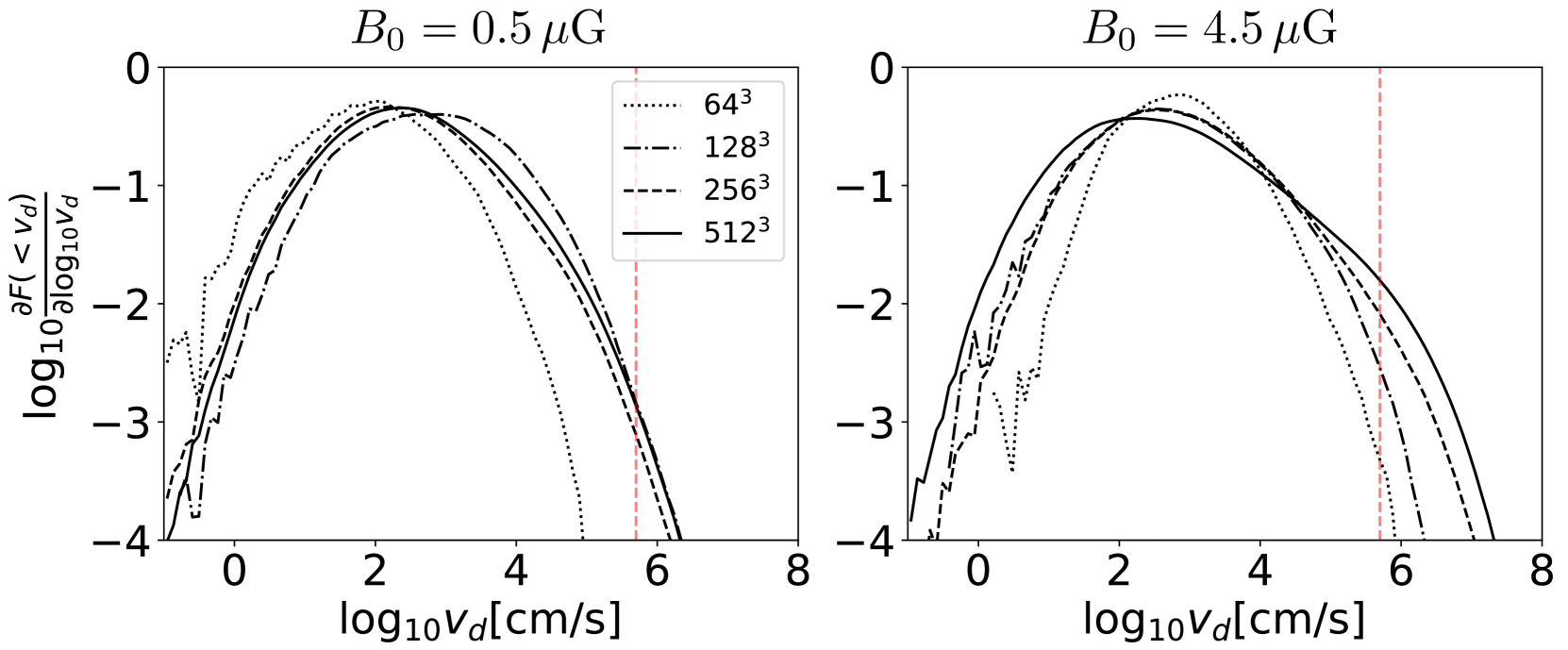
One result of our study has been that the the ion-neutral drift velocity plays a critical role in CH+ formation and excitation of rotational line emisssion. Here we examine the sensitivity of to resolution for our simulations with heating and cooling included throughout and an adiabatic . In figure 17, we show the probability density functions of the ion-neutral drift velocity at four different resolutions, from through , and at two separate mean magnetic field strengths, 0.5 G and 4.5 G. It is worth noting that the highest end of this distribution will never converge in a turbulent domain without ambipolar diffusion being modeled explicitly. This provides additional reason for us to implement a cut in the ion-neutral drift velocities that we consider in our analysis.
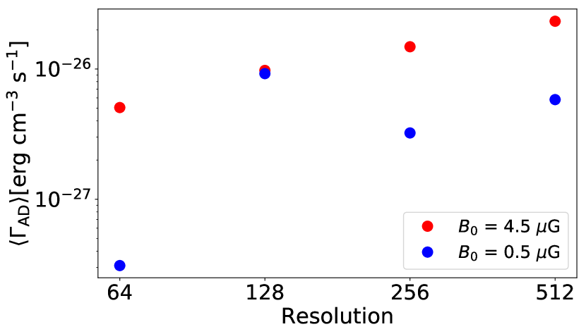
Figure 18 shows the mean ambipolar diffusion heating computed only for cells with ion-neutral drift velocities below 5 km/s. While our results do seem to have some resolution dependence, we would expect this. Only if we were to introduce an explicit physical dissipation mechanism would we expect a well-converged result.
Appendix B Calculating level populations and emission
B.1 Radiative Processes
We seek to calculate the populations of the levels of the electronic ground state . Einstein coefficients for quadrupole transitions between the different levels are taken from Turner et al. (1977).333For all important transitions, these are in agreement with the more recent values from Wolniewicz et al. (1998).
Our code allows for photoexcitation out of the ground electronic state to the , , and states, followed by either dissociation or return to bound levels of the ground electronic state. We use energy levels, Einstein coefficients, and dissociation probabilities from Abgrall & Roueff (1989) and Abgrall et al. (1993a, b). However, the results presented here assume ultraviolet pumping to be weak enough so that excitation is dominated by collisional processes.
B.2 Collisional Rate Coefficients
We include the effects of collisions with , , , and on the rovibrational excitation and deexcitation of . Excitation rates are obtained from deexcitation rates using detailed balance:
| (40) |
where , and for even, odd.
B.3 Statistical Equilibrium
Let be the number density of H nucleons. We consider the bound rotation-vibration levels of with rotational quantum number , and assign level index in order of increasing energy , with corresponding to and to . Let
| (41) |
be the fraction of the H nucleons in , and let
| (42) |
be the fraction of the nucleons in atomic H. We neglect the small fraction of H in molecules other than . The ionized fraction is then .
For we define a transition matrix
| (43) |
where, for
| (44) | |||||
| (45) | |||||
| (46) | |||||
| (47) | |||||
| (48) | |||||
| (49) | |||||
| (50) |
where is the rate per volume of formation on grains, and is the fraction of newly-formed in rotation-vibration state .
For convenience, we define the diagonal elements
| (51) |
Then we have
| (52) |
B.4 Pseudo Steady State
The true steady state solution with for is one where dissociation is balanced by formation. The time scale for approaching this steady state, , is generally long compared to the timescales for redistribution over the vibration-rotation states. In fact, formation and dissociation will often not be balanced in interstellar molecular gas, particularly hot gas that may be cooling rapidly after being shock-heated.
Collisional deexcitation of levels that have been populated by UV pumping and injection of newly-formed in excited states can act as a heat source, confusing the calculation of collisional cooling. To remove the effects of UV pumping and isolate the collisional cooling, we treat the atomic fraction as a parameter, artificially suppress the rate of formation by a factor , and find the solution to the set of equations
| (53) |
where
| (57) |
where the factor modifies all of the dissociation rates to ensure that the steady-state solution to (53) has the desired atomic fraction :
| (58) |
The rates for UV pumping are also suppressed by the factor . Because we take , the H2 level populations are determined only by collisional processes and spontaneous radiative decay.
B.5
Lique (2015) has calculated collisional deexcitation rate coefficients for for the 63 rotation-vibration excited states with (), for temperatures . This includes levels up to , , , and . We use the Lique (2015) deexcitation rates for deexcitation from these levels. For deexcitation from levels , we use the Lique (2015) rates for the same , , and if available; otherwise we use rates for the same and the highest considered by Lique (2015). For we interpolate in the rates provided by Lique (2015). For or we assume the deexcitation rates to scale as .
B.6
For collisional deexcitation we assume that one of the colliding molecules does not change state; this is clearly incorrect, but a full set of state-to-state rate coefficients for collisions is not yet available. We use the inelastic cross sections calculated by Le Bourlot et al. (1999) increased by a factor of 3 to obtain vibrational relaxations rates in agreement with the experimental results of Dove & Teitelbaum (1974) at , , and .
For we use simple analytic fits to the rates calculated by Le Bourlot et al. (1999).
B.7
For collisional deexcitation we use the analytic functions provided by Le Bourlot et al. (1999) to fit their quantum-mechanical results. The results of Balakrishnan et al. (1999) appear to be in good agreement with the Le Bourlot et al. (1999) rates for the transitions that dominate the inelastic collisions.
B.8
We consider only and .
Appendix C Polarization by Aligned Dust Grains
Suppose the dust grains to be oblate spheroids, with cross sections and for parallel and perpendicular to the symmetry axis . Consider directions and in the plane of the sky. In the Rayleigh limit , a dust grain will have cross sections
| (65) | |||||
| (66) |
for radiation with in the and directions, respectively. Let measure the alignment of grain axes with the local magnetic field direction :
| (67) |
Randomly-oriented grains have and ; perfectly-oriented grains have . We assume to be independent of position. Define
| (68) | |||||
| (69) | |||||
| (70) | |||||
| (71) | |||||
| (72) | |||||
| (73) |
Suppose the grains have , with precessing around . Averaging over the precession and along the sightline:
| (74) | |||||
| (75) |
Define
| (76) | |||||
| (77) |
In the Rayleigh limit, an optically-thin sightline has emitted intensity
| (78) | |||||
| (79) |
The Stokes and , and polarized intensity are
| (80) | |||||
| (81) | |||||
| (82) |
Let denote a beam average. The polarized intensity and total intensity are
| (83) | |||||
| (84) | |||||
The beam-averaged fractional polarization is
| (85) |
Aligned grains polarize starlight. Let and be extinction cross sections for starlight polarized parallel or perpendicular to . The “modified picket fence approximation” (MPFA) consists of using Eq. (65,66) even at wavelengths that are comparable to the grain size. Draine & Hensley (2020, in prep.) show that the MPFA is sufficiently accurate to use in modeling starlight polarization. The difference in extinction cross section for radiation polarized perpendicular or parallel to the projection of on the plane of the sky is then
| (86) |
and initially unpolarized radiation develops a polarization characterized by
| (87) | |||||
| (88) |
The fractional polarization of the starlight is
| (89) |