A comparison of quasar emission reconstruction techniques for $z\geq 5.0$ Lyman-$\alpha$ and Lyman-$\beta$ transmission

Abstract

Reconstruction techniques for intrinsic quasar continua are crucial for the precision study of Lyman-$\alpha$ (Ly-$\alpha$) and Lyman-$\beta$ (Ly-$\beta$) transmission at $z>5.5$, where the $\lambda<1215$Å emission of quasars is nearly completely absorbed. While the number and quality of spectroscopic observations has become theoretically sufficient to quantify Ly-$\alpha$ transmission at $5.0<z<6.0$ to better than $1\%$, the biases and uncertainties arising from predicting the unabsorbed continuum are not known to the same level. In this paper, we systematically evaluate eight reconstruction techniques on a unified testing sample of $2.7<z<3.5$ quasars drawn from eBOSS. The methods include power-law extrapolation, stacking of neighbours, and six variants of Principal Component Analysis (PCA) using direct projection, fitting of components, or neural networks to perform weight mapping. We find that power-law reconstructions and the PCA with fewest components and smallest training sample display the largest biases in the Ly-$\alpha$ forest ($-9.58\%/+8.22\%$ respectively). Power-law extrapolations have larger scatters than previously assumed of $+13.1\%/-13.2\%$ over Ly-$\alpha$ and $+19.9\%/-20.1\%$ over Ly-$\beta$ . We present two new PCAs which achieve the best current accuracies of $9\%$ for Ly-$\alpha$ and $17\%$ for Ly-$\beta$ . We apply the eight techniques after accounting for wavelength-dependent biases and scatter to a sample $19$ quasars at $z>5.7$ with IR X-Shooter spectroscopy, obtaining well-characterised measurements for the mean flux transmission at $4.7<z<6.3$. Our results demonstrate the importance of testing and, when relevant, training, continuum reconstruction techniques in a systematic way.

1 Introduction

Hydrogen reionisation is thought to have been powered mostly by the first galaxies and quasars, which by redshift $z\sim 5.5$ were producing sufficient numbers of UV ionising photons to keep the intergalactic medium (IGM) near-completely ionised (Robertson et al., 2013). The timing of reionisation, its progression, and its morphology on both small and large scales are therefore closely tied to the properties of the first sources (e.g. Robertson et al. 2015; Madau & Haardt 2015; Stark 2016; Dijkstra et al. 2016), making reionisation a crucial milestone for both cosmology and galaxy formation.

While the Planck satellite estimated the mid-point of reionisation at $z\simeq 7.65\pm 0.73$ from the optical depth of electron scattering (Planck Collaboration et al., 2020) and upcoming $21$cm experiments promise constraints on the abundance of neutral hydrogen up to $z\lesssim 20$ (Mao et al., 2008; Trott & Pober, 2019), the most accurate measurements currently come from measuring Lyman-$\alpha$ (Ly-$\alpha$) opacity towards $z>5.5$ quasars (Fan et al., 2000, 2006; McGreer et al., 2015) as lower limits. Gunn & Peterson (1965) predicted that the Ly-$\alpha$ forest gives way to completely absorbed ‘Gunn-Peterson troughs’ for IGM neutral fractions $\gtrsim 0.1\%$. Such features have now been detected down to $z\sim 5.6$ (Becker et al., 2015), but the transition from partial IGM transmission to full absorption is complex.

On large scales, the coherence of Ly-$\alpha$ transmission on very large scales ($>160$ cMpc) and the unexpectedly large scatter between quasar sight-lines at the same redshift (Becker et al., 2015; Bosman et al., 2018; Eilers et al., 2018) have ruled out the simplest model of reionisation with a constant UV background (UVB) and inhomogeneities due only to density fluctuations (Songaila, 2004; Lidz et al., 2006). Current models are competing to match observations by incorporating further physical processes, such as a fluctuating mean free path of ionising photons (Davies & Furlanetto, 2016; D’Aloisio et al., 2018), strong temperature fluctuations (D’Aloisio et al., 2015), a contribution from rare sources (Chardin et al., 2015; Meiksin, 2020), or persisting neutral IGM patches (Kulkarni et al., 2019; Nasir & D’Aloisio, 2020; Choudhury et al., 2021). The Lyman-$\beta$ (Ly-$\beta$) forest, which continues to display transmission after Ly-$\alpha$ has saturated, similarly reveals scatter in excess of predictions from density fluctuations alone (Oh & Furlanetto, 2005; Eilers et al., 2019; Keating et al., 2020).

In order to measure Ly-$\alpha$ and Ly-$\beta$ transmission on large scales, it is crucial to accurately predict the intrinsic quasar emission before absorption by the IGM. The near-total absorption at $\lambda_{\text{rest}}<1215$Å (the ‘blue side’) means this requires extrapolation from the quasar rest-UV continuum at $\lambda>1220$Å (the ‘red side’). In the past, this has been been done either via modelling of quasar emission by a power law (e.g. Bosman et al. 2018) or by training the reconstruction at $z<4$ via Principal Component Analysis (PCA) (e.g. Eilers et al. 2018, 2020). The accuracy of power-law reconstructions and PCA techniques is likely to become the leading source of uncertainty in Ly-$\alpha$ transmission studies at $z>5.5$ as the number of known quasars in the reionisation era will soon exceed $1000$ (Ivezić et al., 2019; Brandt & LSST Active Galaxies Science Collaboration, 2007) and deep spectroscopic observations are accumulating (D’Odorico in prep.).

Meanwhile, on small scales, many different statistical techniques are exploiting residual Ly-$\alpha$ transmission at $5.5<z<6.5$ where absorption troughs are punctuated by transmission spikes. As stronger IGM absorption makes it increasingly challenging to measure the Ly-$\alpha$ forest power spectrum directly at $z>5.2$ (Nasir et al., 2016; Oñorbe et al., 2017; Boera et al., 2019), new techniques are instead using the abundance and morphology of residual transmission spikes (Chardin et al., 2018; Gaikwad et al., 2020), the size distribution of absorption troughs (Songaila & Cowie, 2002; Gallerani et al., 2006; Gnedin et al., 2017), the fraction of absorbed pixels (McGreer et al., 2011; McGreer et al., 2015) and correlations of the transmission with galaxies (Becker et al., 2018; Davies et al., 2018a; Kakiichi et al., 2018; Meyer et al., 2019a; Meyer et al., 2020; Kashino et al., 2020). These methods are opening up novel ways to probe the temperature and ionisation state of the IGM and the sources responsible for reionisation, but now rely not only on the accuracy of continuum reconstruction methods but also, to varying extents, to the lack of wavelength-dependence of any residual biases arising during continuum reconstruction.

In this paper, we directly compare the performance of eight quasar reconstruction techniques on a common testing sample of quasars at $2.7<z<3.5$, where the intrinsic emission at $\lambda<1215$Å can be reliably estimated. By carefully characterising the bias and uncertainties of these methods and their wavelength-dependence, we aim to reconcile current measurements of Ly-$\alpha$ opacity at $z>5.5$ and provide a grounding for reconstruction methods in the future.

In Section 2, we detail the continuum reconstruction techniques tested in this work and the related free parameters which include both empirical model-dependent reconstructions and machine-learning techniques. The selection of the test sample and our methods for testing and, when relevant, training the reconstruction methods are given in Section 3. Section 4 presents the results of the analysis in the form of mean biases and uncertainties for each technique and consequences for measurements of the mean Ly-$\alpha$ and Ly-$\beta$ transmission at $z>5$. We summarise in Section 6.

Throughout the paper, we use a Planck cosmology with $h=0.6732$, $\Omega_{m}=0.3158$ (Planck Collaboration et al., 2018). Distances are comoving and all wavelengths are given in the rest-frame of the emitting object unless otherwise specified.

2 Continuum Reconstruction Techniques

Quasar continuum reconstruction techniques used to analyse Ly-$\alpha$ transmission fall into three categories. First, explicitly model-dependent predictions include extrapolating a power-law shape of the spectral distribution function (SED) with best-fit parameters extracted from $\lambda>1220$ Å (Section 2.1) and more complex models which derive empirical correlations between explicit quasar features, such as the shapes and strength of emission lines redwards and bluewards of the Ly-$\alpha$ line (Greig et al., 2017). Second, the largest category is broadly model-independent machine learning techniques, usually in the form of PCA (Section 2.2) but also including more refined Independent Component Analysis (ICA; as used in e.g. Rankine et al. 2020) and neural-network procedures (e.g. Fathivavsari 2020; Liu & Bordoloi 2021). Finally, one may use direct stacks of ‘nearest neighbours’ to individual high-redshift quasars selected from populations of low-redshift quasars using varying (sometimes model-dependent) definitions of proximity (Section 2.3). Examples of the reconstruction techniques are shown in Figure 1 and more examples are available online .

2.1 Power-law extrapolation

Quasar spectra display a wide range of narrow and broad emission lines with high ionisation energies $h\nu\geq 1$ Ry, which are thought to originate from photo-ionisation in accretion disks surrounding a supermassive black hole (SMBH) through processes involving synchrotron emission and Compton scattering of electrons (Krolik & Kallman, 1988). Underneath these emission lines, the mean SED of quasars assumes a comparatively simple power-law dependence, $F_{\nu}\propto\nu^{\alpha_{\nu}}$, over extended stretches of the optical wavelengths ($2000<\lambda<5000$ Å), far UV (FUV; $2000<\lambda(\text{\AA})<1000$) and extreme UV (EUV; $\lambda<1000$Å). Power-law extrapolations from the continuum redwards of Ly-$\alpha$ onto the bluewards side have been the most popular approach to reconstructing quasar intrinsic emission due to the method’s relative simplicity (Fan et al., 2000, 2006; McGreer et al., 2015). The uncertainties of power-law reconstruction have been assumed to be of order $\sim 5\%$ or $\sim 10\%$ (e.g. Fan et al. 2002; Bosman et al. 2018).

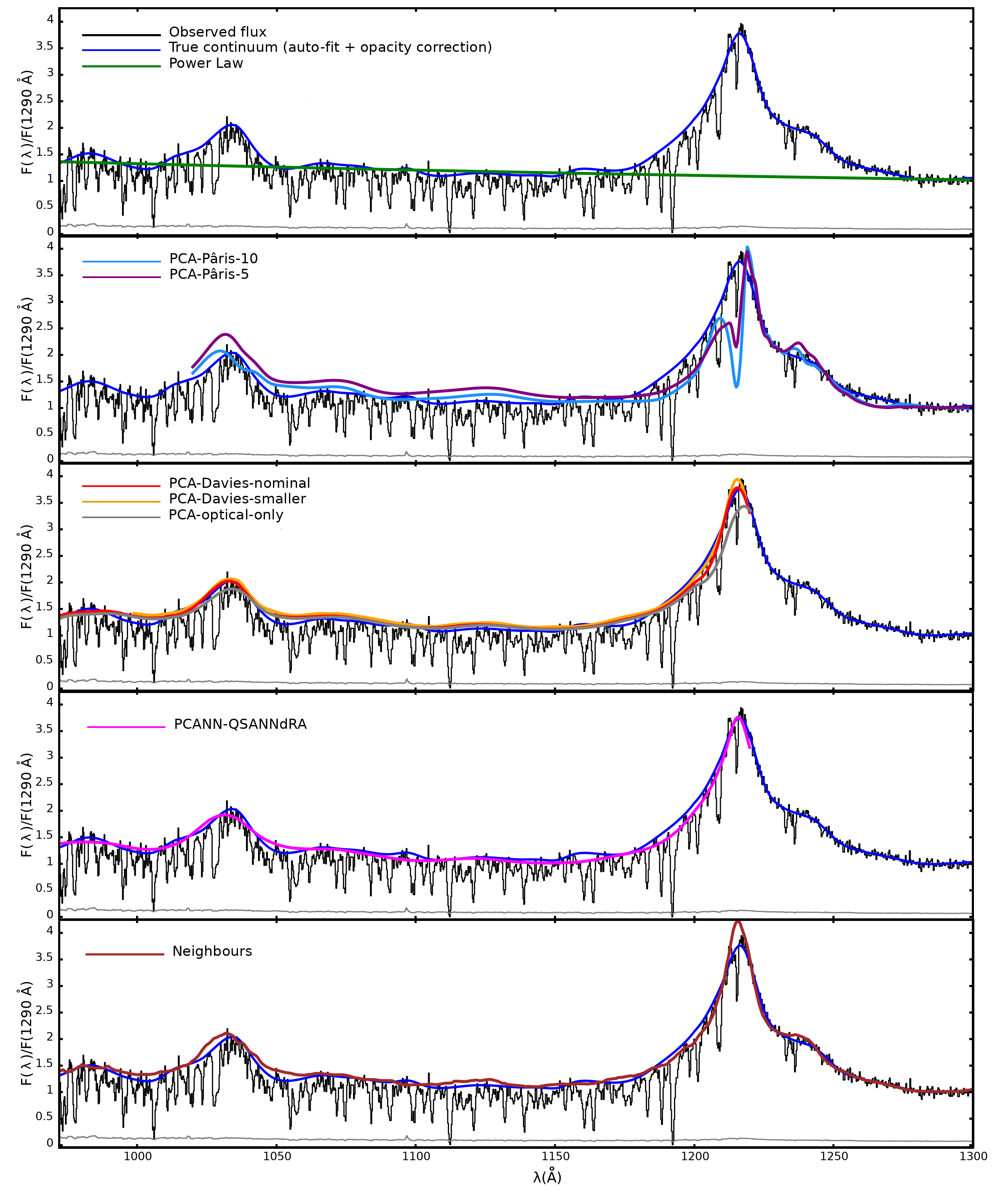
Figure 1: Illustrative comparison of the eight quasar continuum reconstruction techniques on the same quasar, SDSS J131147.52+271826.7 at $z=2.974$. For each method, models are fit on the red side ($\lambda\geq 1240$Å) and used to make the predictions of the blue side ($\lambda\leq 1290$Å) shown in the five panels. The dark blue line shows the automatically-recovered continuum, used for testing the predictive accuracy of the models. The new PCAs were not trained to reproduce the shape of the Ly-$\alpha$ line.

There is evidence for a break in the power-law form of quasar SEDs around the optical/FUV or FUV/EUV divisions. Richards et al. (2001) analysed composite spectra from the Sloan Digital Sky Survey (SDSS, Fukugita et al. 1996), finding slopes $\alpha_{\nu}\simeq-0.5$ over $1300<\lambda<5000$Å. In contrast, studies of FUV and EUV quasars SEDs find much steeper slopes $\alpha_{\nu}\sim-1.7$ over $500<\lambda(\text{\AA})<1200$, with potential dependences of $\alpha_{\nu}$ on quasar luminosity and radio-loudness (Telfer et al., 2002; Scott et al., 2004). In a homogeneous analysis of the EUV, FUV and optical continua, Shull et al. (2012) find roughly constant SED slopes over $2000<\lambda(\text{\AA})<5000$ of $\alpha_{\nu,\text{opt}}=-0.3$, which steepen significantly towards the FUV around $\lambda\sim 2000$Å to $\alpha_{\nu,\text{FUV}}=-1.4$ and again towards the EUV at $\lambda=1000\pm 50$Å to $\alpha_{\nu,\text{EUV}}=-2.0$. If this is the case, extrapolations from the red side of Ly-$\alpha$ , $\lambda\gtrsim 1270$Å, are expected to become increasingly biased at shorter wavelengths $\lambda<1000$Å. Furthermore, power-law extrapolations do not capture the broad quasar lines superimposed on the continuum emission, which may give rise to strong wavelength-dependent biases. The characteristic velocity separations between broad lines give rise to spurious correlations on specific scales, which may be important to $z>5.5$ Ly-$\alpha$ studies in similar ways to $z<5.0$ (e.g. Lee et al. 2012; McDonald et al. 2006; Oñorbe et al. 2017).

In order to quantify the bias, we closely reproduce the procedure employed at $z>5.5$. The free parameters are the wavelength range being used, usually $1270\lesssim\lambda\lesssim 1450$ Å, and the number of fitting iterations after masking of non-continuum pixels i.e. ‘sigma-clipping’. Although this spectral range is less abundant in broad emission lines than longer wavelengths $\lambda>1450\AA$, it is nevertheless affected by the Si II $1303$, O I $1307$, C II $1335$, Si IV $1396$ and O IV] $1404$ Å broad lines (all of which are in fact doublets or triplets with separations $\gtrsim 10$ times smaller than their typical widths). Furthermore, the broad emission lines show non-trivial velocity shifts with respect to the quasar’s systemic redshift and to each other (Greig et al., 2017; Meyer et al., 2019b) and the quasar redshifts estimated by the BOSS pipeline can be inaccurate by up to $\Delta z\simeq 0.05$ (Hewett & Wild, 2010; Coatman et al., 2016). It is therefore not feasible to fit a power-law continuum solely ‘in-between’ the broad lines and iterative rejection criteria are employed instead.

In this work, we fit power-laws of the form $\text{PL}(\lambda)=k\lambda^{\alpha_{\lambda}}$ with $\alpha_{\lambda}=-(\alpha_{\nu}+2)$. We employ the full range $1270<\lambda(\text{\AA})<1450$ with three rounds of outlier rejection at $|F(\lambda)-\text{PL}(\lambda)|>3\sigma,2.5\sigma,2\sigma$. We find these exclusion criteria to be necessary and sufficient for fit convergence, and we illustrate the effect of changing the fitting wavelength range in the Appendix A.

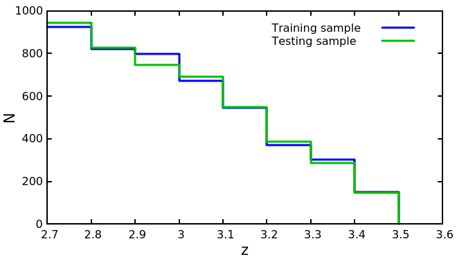
Figure 2: Redshift distribution of the training and testing samples. Both samples contain $4597$ quasars and the objects were divided randomly.

0

2.2 Principal Component Analysis

Quasar spectra are a good target for PCA analyses due to their strong correlated spectral features: $\sim 75\%$ of their observed optical/UV spectral properties can be captured with linear combinations of only $\sim 3$ components (Francis et al., 1992; Yip et al., 2004; Suzuki et al., 2005; McDonald et al., 2005). We outline here the principles of PCA decomposition and reconstruction, before giving more details on the specific PCAs used in our comparison in the following subsections. The steps involved in producing and applying a PCA reconstruction for the Ly-$\alpha$ transmission continuum are:
(1) The identification of an appropriate training sample of N quasars for which the true underlying continuum $q(\lambda)$ at $\lambda<1220$ Å (the blue side) and $\lambda>1220$Å (the red side) can be accurately determined. The determination of $q(\lambda)$ can be manual or automated, and is usually different on the red side and the blue side (where the Ly-$\alpha$ forest requires special treatment) with a continuity requirement at the interface.
(2) Decomposing both the red side continuum and the total (red and blue) continuum ($q(\lambda)$ into their principal components. Mathematically, this equates to computing the covariance matrix $\mathbb{C}$:

$$\mathbb{C}(i,j)=\frac{1}{N-1}\sum_{n=1}^{N}\left(q_{n}(\lambda_{i})-\bar{F}(\lambda_{i})\right)(q_{n}(\lambda_{j})-\bar{F}(\lambda_{j})),$$ (1)

where $\bar{F}(\lambda)$ is the mean quasar flux over the entire training sample. One then finds the matrix $\mathbb{P}$ which diagonalises $\mathbb{C}$ i.e. such that $\mathbb{C}=\mathbb{P}^{-1}\times\mathbf{\Lambda}\times\mathbb{P}$ where $\mathbf{\Lambda}$ is diagonal. The columns of $\mathbb{P}$ contain the eigenvectors/principal components $p_{i}(\lambda)$.
(3) The mapping between the red side and the total spectrum is computed via the projection matrix $\mathbb{X}$. To do this, the weight matrices $\mathbb{W}$ on both sides are computed over all quasars in the training sample via

$$\mathbb{W}_{ij}=\int\left(q_{i}(\lambda)-\bar{F}(\lambda)\right)p_{j}(\lambda)d\lambda$$ (2)

and finally the projection matrix is found in order to map between the sides: $\mathbb{W}_{\text{red+blue}}=\mathbb{X}\times\mathbb{W}_{\text{red}}$. At this stage, the number of principal components on both sides is customarily truncated to retain only those which account for most of the variance, although the criteria for defining this cut-off vary widely.

Figure 3: SNR Distribution of the quasar spectra in the training and testing samples, measured at $1290\pm 5$Å. $\sim 1\%$ of objects in both samples have SNR $>30$. Both samples contain $4597$ quasars and the objects were divided randomly.

Armed with the mean flux $\bar{F}(\lambda)$, the two sets of principal components $p_{i}(\lambda)_{\text{red}}$ and $p_{i}(\lambda)_{\text{red+blue}}$ and the projection matrix $\mathbb{X}$, one can now make a prediction of the blue continuum for any new quasar outside the training set as follows:
(4) Extract the red-side continuum $q_{r}(\lambda)$ of the new quasar with the same technique as used in step (1).
(5) Project or fit the set of components weights $w_{i,r}$ such that $q_{\text{red}}(\lambda)-\bar{F}(\lambda)=\sum_{i}w_{i,r}p_{i,\text{red}}(\lambda)$. In theory, this can be achieved cleanly via projection of $q_{\text{red}}(\lambda)$ in the basis of the $p_{i,\text{red}}(\lambda)$:

$$w_{i,r}=\int\left(q_{\text{red}}(\lambda)-\bar{F}(\lambda)\right)p_{i,\text{red}}(\lambda)d\lambda;$$ (3)

but in practice, the truncation of the principal components at step (3) and the desire to obtain uncertainties on the weights $w_{i,r}$ means that direct fitting in wavelength space is very frequently used instead.
(6) The vector of weights on the red+blue sides, $\mathbf{w_{r+b}}$, is obtained from the weights on the red side, $\mathbf{w_{r}}$, by multiplying with the projection matrix, $\mathbf{w_{r+b}}=\mathbb{X}\mathbf{w}_{r}$. The continuum prediction is given by $\text{Pred}(\lambda)=\bar{F}(\lambda)+\sum_{i}w_{i,r+b}p_{i,\text{red+blue}}(\lambda)$.

Although important differences between PCA methods occur at stages (1), (3) and (5) as will be discussed below, the most crucial difference is in the choice of training sample in step (1). Quasars at $z>6$ have shown signs of intrinsic evolution compared to $z<5$, displaying extreme velocity shifts of the highly-ionised broad emission lines more frequently at early times at equal quasar luminosity (Shen et al., 2008; Richards et al., 2011a; Mazzucchelli et al., 2017; Meyer et al., 2019b; Shen et al., 2019). It is therefore extremely important that the training sample for PCA be large enough to capture the relatively rare analogue objects at $z<5$. If extreme broad line shifts are caused by a distinct physical process, it is also crucial that sufficient principal components are retained at step (3) to adequately describe this population. Finally, one should be wary that the continuum fitting at steps (1) and (4) be not biased against quasar spectra with strong line shifts, weak emission lines, or lower signal to noise ratios (SNR). PCA is trained directly to reproduce the intrinsic continua recovered in step (1). For example, the presence of strong damped Ly-$\alpha$ absorbers (DLAs) which are not correctly excluded from the training continuum fitting will introduce random features which PCA cannot match and reduce its predictive power. To illustrate the cumulative importance these effects, we test two models which differ solely in step (1): PCA-Davies-smaller and PCA-Davies-nominal (Section 2.2.2).

2.2.1 Classical quasar PCA

The first PCA reconstruction we test is through the components of Pâris et al. (2011) (P11), which have previously been used to study Ly-$\alpha$ transmission at high-$z$ (Eilers et al., 2017; Eilers et al., 2018). P11 provide $10$ principal component vectors for both the $1020<\lambda(\text{\AA})<2000$ (total) range and the $1216<\lambda<2000$Å (red) range, as well as a projection matrix for linking the two. Their training sample consists of 78 quasars at $2.82<z<3.00$ from SDSS-DR7. The quasars were selected to have SNR $>14$ over the red-side continuum, and the sample was manually cleaned to avoid any broad absorption line (BAL) quasars, any DLAs, and any spectra with reduction issues. The continua were fit with a spline manually. P11 estimated the uncertainty in predicting the Ly-$\alpha$ forest continuum via the ‘leave one out’ method, i.e. training on 77 quasars and evaluating the prediction on the 78${}^{\text{th}}$. P11 report uncertainties of $9.5\%$ at the 90${}^{\text{th}}$ percentile. To test the prediction on a larger collection of quasars, we automate the continuum spline fitting while retaining the ban on BAL quasars (see Section 3.2). Following P11, we use all $10$ components and conduct weight determination (step (5) above) via re-binning and direct projection. We label this method PCA-Pâris-10 in the rest of the paper.

Quasar name	$z_{\text{sys}}$	SNR	Ref.
J1120+0641	7.085	48	Mortlock et al. (2011)
PSOJ011+09	6.4693	17	Mazzucchelli et al. (2017)
J0100+2802	6.3258	119	Wu et al. (2015)
J1030+0524	6.3000	35	Fan et al. (2001)
J0330-4025	6.239	13	Reed et al. (2017)
PSOJ359-06	6.1718	41	Wang et al. (2016)
J2229+1457	6.1517	11	Willott et al. (2010)
J1319+0950	6.1333	104	Mortlock et al. (2009)
J1509-1749	6.1225	66	Willott et al. (2007)
PSOJ239-07	6.1098	36	Bañados et al. (2016)
J2100-1715	6.0806	30	Willott et al. (2010)
PSOJ158-14	6.0681	38	Chehade et al. (2018)
J1306+0356	6.0332	77	Fan et al. (2001)
J0818+1722	6.00	135	Fan et al. (2006)
PSOJ056-16	5.967	54	Bañados et al. (2016)
J0148+0600	5.923	139	Jiang et al. (2015)
PSOJ004+17	5.8165	27	Bañados et al. (2016)
J0836+0054	5.810	85	Fan et al. (2001)
J0927+2001	5.772	93	Fan et al. (2006)

Table 1: Quasars included in the computation of the mean Ly-$\alpha$ and Ly-$\beta$ transmitted flux at $z>5$, selected to have IR X-Shooter spectra with BOSS-equivalent SNR $>7$.

Using the P11 PCA components to reconstruct the continua of $z>5.5$ quasars, Eilers et al. (2017) noticed that restricting the fit to only the first $7$ or $5$ PCA components gave a qualitatively better fit to the red side in every case for their sample of $34$ quasars. One possible explanation is the presence of redshift errors in the P11 training sample, which components $6$ to $10$ seem predominantly designed to correct. To adjust to this difference, Eilers et al. (2017) opt to use the first $3$, $5$ or $7$ components of the P11 PCA depending on the qualitative appearance of the red-side fit, and use the PCA components from Suzuki (2006) instead on $7$ quasars where none of those options were satisfactory. This more careful process is difficult to automate, so we choose to only test the $5$-component fit which was used most commonly ($\sim 59\%$) for their sample. Following Eilers et al. (2017), we conduct weight determination via $\chi^{2}$ fitting and label this technique PCA-Pâris-5. We indeed find the fits with only $5$ components to be qualitatively different from fits using all $10$ (see e.g. Figure 1). It is important to note the PCA’s projection matrix is not re-trained when changing the number of components, but only truncated.

2.2.2 New quasar PCA

The SDSS-III Baryon Oscillation Spectroscopic Survey (BOSS) and the SDSS-IV Extended BOSS (eBOSS) obtained low resolution ($R\sim 2000$) spectra of the Ly-$\alpha$ forest of over $290,000$ quasars at $2<z<5$ (Dawson et al., 2013, 2016). Davies et al. (2018c) (D18) leveraged the SDSS-DR12 BOSS quasar catalogue (Pâris et al., 2017) to create new quasar PCA decompositions, following the steps described above with a few modifications. D18’s original training sample includes $12,764$ quasars with $2.09<z<2.51$ and SNR $>7.0$ and is relatively devoid of BALs and wrong quasar identifications by virtue of the visual inspection flags in the SDSS DR12 quasar catalogue. New additional BAL exclusion methods were also introduced. The red and blue sides of the continuum are split entirely into $\lambda<1220$Å and $\lambda>1220$Å instead of predicting the overall continuum in step (2). The method implements a continuity condition at the interface, and fitting is performed with an automated spline fitter similar to the one in this paper but without explicit DLA masking (see Section 3.2). Two major additions to the procedure in Section 2.2 are:

• The PCA-building and fitting procedures are conducted in flux log space, using $\text{log}(F(\lambda))$ instead of $F(\lambda)$. This enables the power-law component of the quasar continuum to be more naturally represented by an additive component, rather than a multiplicative one.

• At the fitting stage, a small shift in redshift ($|\delta z|<0.05$) is fit at the same time as the PCA component weights. Consequently, weight determination is always conducted via $\chi^{2}$ minimisation.

The original PCA in D18 was aimed at predicting the shape of the Ly-$\alpha$ emission line rather than the bluewards continuum (Davies et al., 2018b; Wang et al., 2020). Prediction errors at $\lambda\sim 1210$ Å were estimated to be around $6-12\%$. To predict the Ly-$\alpha$ forest continuum, we shift the dividing point between the red and blue sides from $\lambda=1280$Å to $\lambda=1220$Å in order to access more emission line properties.

We test three versions of the PCA generated using D18’s procedure, all using $10$ red-side components and $6$ blue-side components. The first version is trained on BOSS DR12, employing $2352$ spectra with SNR $>10$ at $2.65<z<3.00$ covering the range $972<\lambda(\text{\AA})<2500$. The intrinsic continuum fitting is the same as in D18 and the fluxing correction described in Margala et al. (2016) has been applied to address a newly-known issue with blue quasar slopes in BOSS DR12. We label this method PCA-Davies-smaller.

Secondly, we train a new PCA following D18’s methodology but using our common quasar training set with $4579$ quasars based on the larger eBOSS-SDSS DR14 catalogue (see Section 3.1). Crucially, this PCA is trained using the same continuum recovery algorithm on the blue side as we use for testing the PCA’s predictive performance. The contrast between these two versions illustrates the variance in PCA predictive performance arising purely from sample size, sample purity, and the recovery of the blue-side continuum. We label this method PCA-Davies-nominal.

Thirdly, we test a PCA identical to the previous one in all points, but using a restricted wavelength range of $972<\lambda(\text{\AA})<1450$. Spectra of $z>5.7$ quasars are frequently only available in the observed-optical wavelengths, in which case only a power-law reconstruction can be used. We therefore wish to test whether PCA can outperform power-law reconstructions under this constraints. We label this method PCA-optical only.

2.2.3 Neural-network-mapped quasar PCA

The final version of PCA we implement is the neural-network-mapped quasar PCA-fitting algorithm PCANN-QSANNdRA described in Ďurovčíková et al. (2020). Like the previous technique, PCANN-QSANNdRA was originally designed to predict the shape of the Ly-$\alpha$ emission line rather than the bluewards continuum. The training sample included $13,703$ quasars from eBOSS DR14 over $2.09<z<2.51$ and SNR $>7$ (Pâris et al., 2018). The continuum was smoothed using a custom routine which employed a random forest to tag intervening absorbers and exclude quasars with strong DLAs. The red side ($1290<\lambda(\text{\AA})<2900$) and the blue side ($1191.5<\lambda(\text{\AA})<1290$) of the continuum are described by $63$ and $36$ PCA components, respectively, with the number of components chosen to contain $99\%$ of the variance in the training sample. The red and blue sides are completely separated, as in D18.

Instead of the weights of the PCA component vectors being mapped linearly following Equation (2), the translation between the blue and red side weights is performed by a four-layered fully connected neutral network. This method introduces an extra step of ‘double standardisation’ whereby the mean across the training sample is subtracted at each wavelength before and after PCA composition, and divided by the error array. The prediction uncertainties were calculated by a committee of $100$ independently-trained neural networks. No simultaneous fitting of a shift in redshift is performed. Owing to the freedom to enact non-linear mapping of PCA coefficients, PCANN-QSANNdRA slightly outperformed D18’s PCA method with uncertainties of $\sim 6-10\%$ at $\lambda\sim 1210$Å.

In this paper, we use an identical methodology to train a neural-network-mapped PCA to reproduce the continuum bluewards of Ly-$\alpha$ using the eBOSS DR14 common training and testing samples described in Section 3.1. As in Ďurovčíková et al. (2020), we use a $50:50$ split for training and validation (both within the eBOSS training sample) and adapt the network to predict the Lyman-series continuum using an identical procedure. In order to capture $99\%$ of the variance, we find that $53$ PCA components are needed for the red side and $42$ for the blue side. The optimal architecture in Ďurovčíková et al. (2020) consisted of four layers with $53-40-40-42$ neurons each, a batch size of $500$ (corresponding to the number of training samples passed through the network before the weights get updated), and $80$ training epochs. To optimise training, we first adjusted the loss function so that prediction errors around $\lambda\sim 1040$Å and $\lambda\sim 1215$Å are weighed more heavily to anchor the prediction where the scatter is largest. The ability to adjust training loss function weights in this manner makes neural-network-mapped quasar PCAs more flexible than standard PCA. We then performed a four-dimensional grid search over the number of neurons in the middle two layers, the batch size, and number of training epochs. The optimal architecture consisted of layers with $53-45-45-42$ neurons, batch size of $500$, and $80$ training epochs. Compared to the original architecture, the optimal one reduced the mean bias below $1\%$ (potentially driven mainly by the updated loss function) but had almost no impact on reducing the prediction error ($<0.2\%$ difference). More details of the neural network architecture and training procedure are given in Ďurovčíková et al. (2020), section 2.3.

2.3 Nearest Neighbours

Stacks of $z<3.0$ quasar spectra are often used to predict the intrinsic emission of $z>5$ quasars and capture features such as broad emission lines in a model-independent way (e.g. Vanden Berk et al. 2001; Cool et al. 2006; Simcoe et al. 2011). Stacks specifically tailored from ‘neighbours’ which match specific features of the red side, such as strong blueshift of the broad C IV emission line, have been shown to perform better than blind stacks (Mortlock et al., 2011; Bosman & Becker, 2015) since those features are known to correlate with properties on the blue side (Baldwin, 1977; Richards et al., 2011a; Greig et al., 2017).

We systematically test the performance of stacks of nearest neighbours for predicting intrinsic emission. To select neighbours, we first fit all quasars with continua on the red side using an automatic spline fitter with fixed point spacing of $\sim 1000$km s^-1, rejecting metal absorbers as described in 3.2. In the absence of Ly-$\alpha$ forest absorption, we find this point spacing better captures the shape of the emission lines (a point spacing of $\sim 1700$km s^-1 was used to fit the blue side). For each quasar $q_{i}$ in the testing sample, the Euclidean distance $d_{i,j}$ to all quasars in the training sample $q_{j}$ is then computed over the red side, $1220<\lambda(\text{\AA})<2000$,

$$d_{i,j}=\sqrt{\sum\limits_{\lambda>1220\text{\AA}}\left(q_{i}(\lambda)-q_{j}(\lambda)\right)^{2}},$$ (4)

in order to identify the $40$ quasars from the training sample with the smallest $d_{i,j}$. The known blue-side continua of the neighbours are then interpolated onto a common wavelength array and averaged. The distance between spectra could be defined in different ways, e.g. weighting more heavily emission lines known to correlate with blue side properties, or calculating the distance after subtracting a power-law fit first. These differences will be most important when the number of neighbours of a specific quasar is limited, and we leave a detailed exploration to future work.

$z$	$z_{\text{mean}}$	$\int dz$	$\langle F\rangle_{\text{{PCA-nominal}}}$	$\langle F\rangle_{\text{{QSANNdRA}}}$
Ly-$\alpha$
$4.7-4.9$	$4.826$	$0.489$	$0.1856_{-0.0132}^{+0.0126}$	$0.1974_{-0.0144}^{+0.0140}$
$4.9-5.1$	$5.015$	$1.826$	$0.1258_{-0.0046}^{+0.0045}$	$0.1330_{-0.0048}^{+0.0049}$
$5.1-5.3$	$5.201$	$2.848$	$0.0991_{-0.0031}^{+0.0031}$	$0.0979_{-0.0032}^{+0.0032}$
$5.3-5.5$	$5.399$	$3.194$	$0.0765_{-0.0025}^{+0.0024}$	$0.0742_{-0.0026}^{+0.0026}$
$5.5-5.7$	$5.596$	$2.804$	$0.0435_{-0.0021}^{+0.0021}$	$0.0432_{-0.0022}^{+0.0022}$
$5.7-5.9$	$5.789$	$2.022$	$0.0236_{-0.0024}^{+0.0024}$	$0.0222_{-0.0025}^{+0.0024}$
$5.9-6.1$	$5.981$	$0.778$	$0.0115_{-0.0036}^{+0.0036}$	$0.0117_{-0.0036}^{+0.0036}$
$6.1-6.3$	$6.188$	$0.290$	$<0.0131$	$<0.0133$
Ly-$\beta$
$5.5-5.7$	$5.605$	$0.719$	$0.0534_{-0.0081}^{+0.0080}$	$0.0601_{-0.0076}^{+0.0086}$
$5.7-5.9$	$5.801$	$1.321$	$0.0358_{-0.0042}^{+0.0042}$	$0.0425_{-0.0042}^{+0.0046}$
$5.9-6.1$	$5.979$	$0.732$	$0.0181_{-0.0029}^{+0.0029}$	$0.0179_{-0.0028}^{+0.0031}$

Table 2: Redshift intervals, mean redshifts, and effective redshift length probed by the sample of $z>5.7$ quasars. We only report redshift bins with $\int dz>1$. Limits are given at the $2\sigma$ level.

3 Methods

We aim to test the quasar continuum predictions described in Section 2 in a consistent way and on a common sample. Each method is applied in a similar way as previous work, and the PCA methods requiring training samples (PCANN-QSANNdRA and PCA-Davies-nominal) are trained on the same sample. Section 3.1 describes the selection of the training and testing samples from the eBOSS DR14 catalogue. We then compare predictions to an automatic continuum-tracer bluewards of the Ly-$\alpha$ emission line. Because we predict the Ly-$\beta$ continuum down to $\lambda=972$Å, we need to use quasars with $z>2.7$ for which the Ly-$\alpha$+Ly-$\beta$ forest absorption is dense. We use an automated spline fitter for the Ly-$\alpha$ forest with masking of individual absorbers, which we describe in Section 3.2. The estimation of the methods’ biases and uncertainties is described in Section 3.4 and their application to $z>5.5$ Ly-$\alpha$ and Ly-$\beta$ opacities in Section 3.5.

3.1 Training and testing sample selection

The selection of the training and testing samples is conducted from the eBOSS DR14 quasar catalogue using the igmspec module of the specdb interface (Prochaska, 2017). We use quasars in the redshift range $2.7<z<3.5$ to ensure coverage of the Ly-$\beta$ forest in the BOSS camera spectral observed wavelength range of $3600<\lambda_{\text{obs}}(\text{\AA})<10400$ (Smee et al., 2013), while IGM absorption becomes too strong beyond $z>3.5$ to enable secure recovery of the true continuum.

We impose a cut of SNR $>7$ at $\lambda=1290$Å to ensure that both the red and blue side can be fit with a spline continuum even in the presence of a high spectral slope. The eBOSS catalogue contains $8118$ objects with those criteria according to the automated pipeline. However, we perform our own calculation of SNR over the $1285<\lambda(\text{\AA})<1295$Å spectral window after masking sky-lines and identify $12,597$ objects instead.

As opposed to the BOSS DR12 catalogue, eBOSS DR14 was not inspected visually and lacks specific data quality flags for BAL quasars. We conduct an automated search for BALs as follows. First, we fit each spectrum with an automated spline with initial fixed points in $\sim 7.5\AA$  intervals, corresponding to $1700$ km s^-1. We use the fitting procedure developed by Young et al. (1979) and Carswell et al. (1982) as implemented by Dall’Aglio et al. (2008), without masking of absorbers. We then normalise the spectra based on the value of the continuum at $\lambda=1290$Å, $F(1290)$. Finally, we cut from the sample any quasars whose automated fit drops below $F/F(1290)=0.2$ across $1220<\lambda(\text{\AA})<1950$ or below $F/F(1290)=0.7$ over the $1290<\lambda(\text{\AA})<1570$ window, which would correspond to a C IV BAL ($1164$ objects or $9\%$ of the sample). Using the same wide-spline fit, we identify strong absorption features which would impair the continuum recovery on the blue side as objects whose continuum drops below $F/F(1290)=0.5$ over $972<\lambda(\text{\AA})<1220$ ($2104$ objects or $17\%$ of the sample). This occurrence rate is a factor $\sim 3$ higher than expected for DLAs alone at $z\sim 3$ (e.g. Prochaska et al. 2009; Crighton et al. 2015), suggesting we are also excluding weaker Lyman-limit systems. We further exclude any quasar with missing flux information over $\geq 7$ consecutive spectral pixels ($34$ objects).

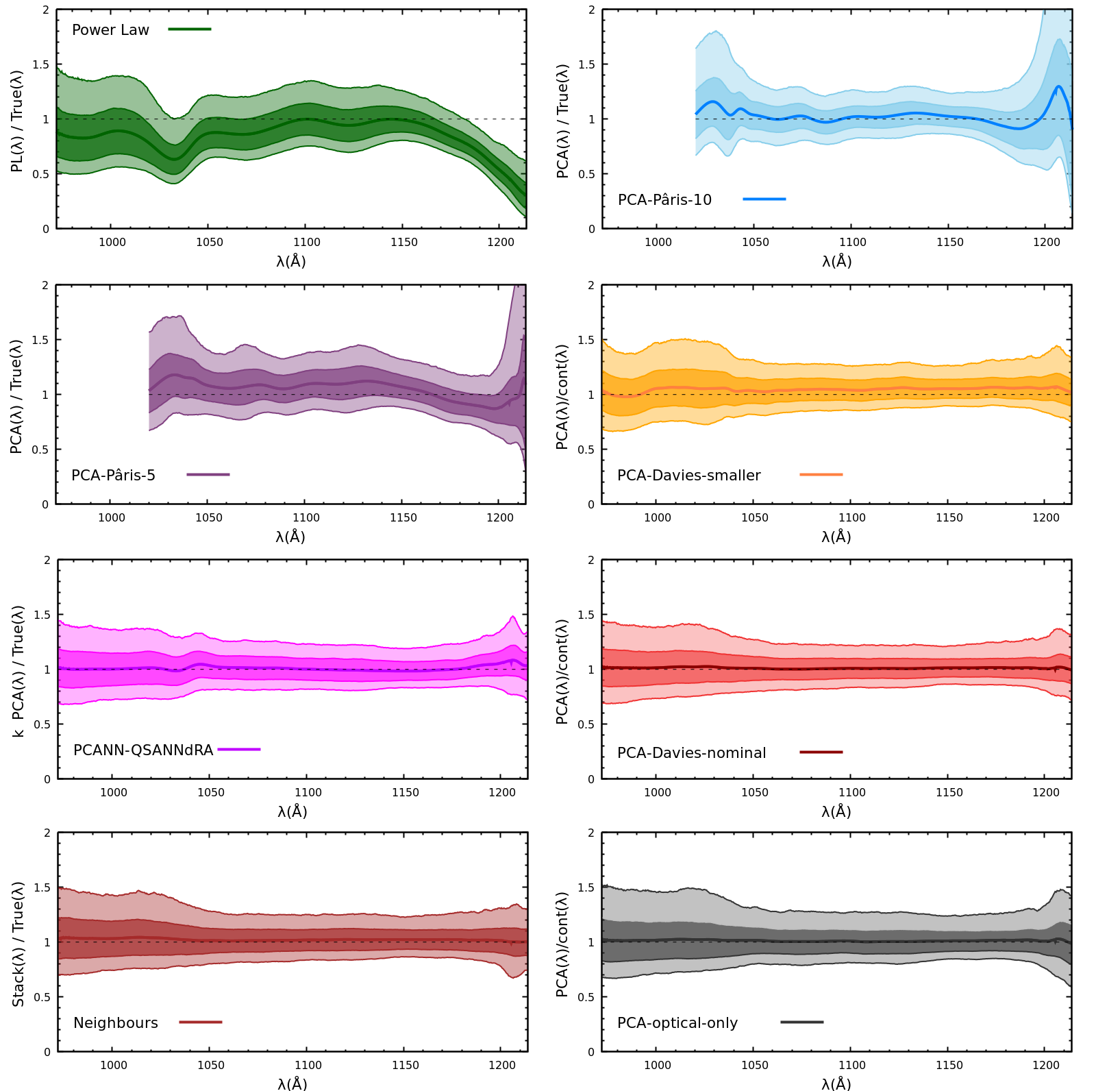
Figure 4: The mean error (bias) in continuum prediction for eight quasar emission reconstruction methods, evaluated over the testing sample of $4579$ quasars at $z<3.5$. The shaded regions correspond to two-sided 1 and 2$\sigma$ contours containing 68% and 95% of the scatter in prediction error. The Power-Law, PCA-Pâris-10, PCA-Pâris-5, Neighbours predictions are compared to the true continuum, i.e. the automated continuum corrected for IGM absorption at $z\sim 2.6$ by a multiplicative constant. The PCA-Davies models are compared to the continuum recovery on which they were trained. The PCANN-QSANNdRA method is compared to the true continuum, divided by a constant $k$ accounting for the different IGM absorption biases of automatic continuum recovery.

Finally, we perform visual inspection of the remaining quasars to exclude incorrect pipeline identification or redshifts. We identify $114$ objects with redshift errors (usually due to mis-identification of the Mg II line as Ly-$\alpha$), $18$ quasars with proximate DLAs too strong to use and $5$ extra BAL quasars not caught by our automated procedure due to the absorption having width $\Delta v<1000$ km s^-1. The final sample contains $9158$ usable quasars, that are divided randomly and evenly into a testing sample of $4597$ objects and a training sample of $4597$ objects. The redshift and SNR distributions of the samples are shown in Figure 2 and Figure 3, respectively.

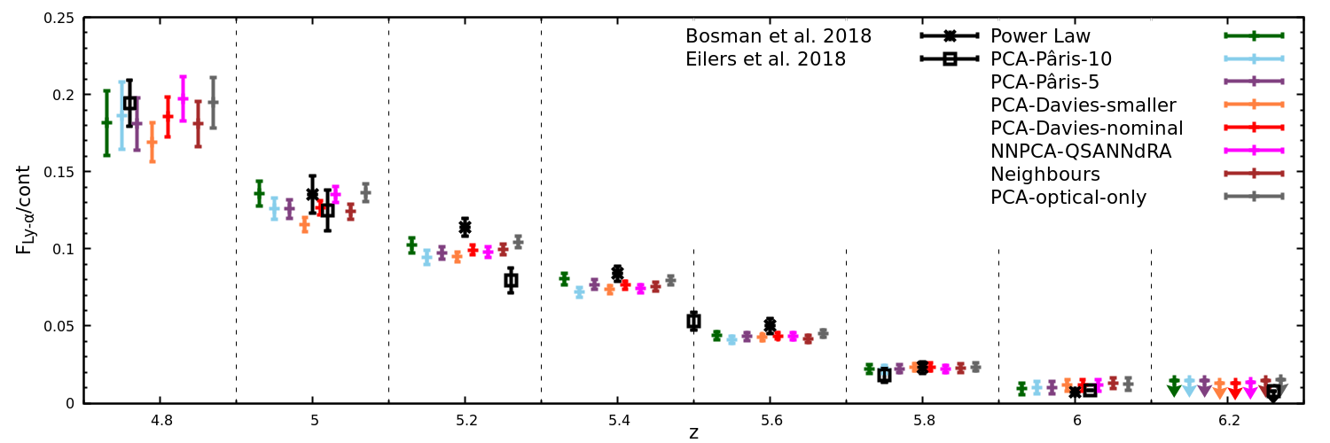
Figure 5: Mean transmitted Ly-$\alpha$ flux along the sightlines of quasars at $z>5.7$. The coloured points correspond to predictions made from eight reconstruction methods, with bias corrections applied from testing on the $2.7<z<3.5$ eBOSS testing sample. Each set of coloured points correspond to stack in redshift between the dotted lines. The uncertainties account for both the $1\sigma$ uncertainties in reconstruction accuracy and observational errors. All techniques agree within $1.5\sigma$. The measurements from Eilers et al. (2018) and Bosman et al. (2018) use different samples and a different binning of $\Delta z=0.25$ and $0.2$, respectively.

3.2 Continuum fitting

We use the following procedure for recovering the underlying quasar continuum on the blue side. Quasar emission lines in the Ly-$\alpha$ and Ly-$\beta$ forest: N III 990 Å, O VI 1033Å, N II 1085Å, Fe III 1125Å and C III 1175Å, are more widely spaced and broader on average than emission lines on the red side (Shull et al., 2012). We therefore start with fitting a spline to the spectrum with initial fixed points $\sim 1700$ km s^-1 intervals as above (more specifically, $25$ pixels in the wavelength array). The spline-fitting procedure of Dall’Aglio et al. (2008) iteratively excludes individual pixels within the bins which have the largest negative deviations from the fit via asymmetric sigma clipping. Convergence is achieved when the standard deviation of the retained flux pixels is below the average observed noise in each bin.

However, we find that the fit has a tendency to return unphysical “wiggles” when it interpolates over absorbers with $\Delta v\gtrsim 0.5$ of the distance between fixed points due to the procedure being stuck to its ‘first guess’ even after all the absorbed pixels are masked. To circumvent this, we implement a more drastic absorber-masking procedure and run the fitter again after explicitly removing all information on pixels identified as absorbers after a first pass. Additionally, we use a stringent requirement that $>40\%$ of all pixels in a bin must be un-masked in order for that bin to factor into the fitting at all. We find the resulting continuum recovery to be far better at interpolating across strong H I absorbers, yet nearly identical to the old procedure in their absence (Appendix C).

The automatic continuum fitting introduces a non-zero intrinsic scatter on the recovered ‘true’ continua arising from stochasticity in the fit quality. Dall’Aglio et al. (2009) estimate this scatter to be $\sim 2.5\%$ at $z=3$. The authors note that the procedure also introduces wavelength-dependent biases of order $2-3\%$, mostly by occasionally under-estimating the continuum over the O VI line when its peak coincides with Ly-$\alpha$ absorption. We expect the improvements made to the method, as described above, should reduce these biases. The extra scatter from the automatic continuum fitting is sub-dominant compared to the measured continuum prediction scatter (Section 4) and we do not consider it further. Wavelength-dependent biases in the procedure are potentially an issue, especially considering that four of the reconstruction methods used different procedures to determine the ‘true’ continua (PCA-Pâris-10, PCA-Pâris-5, PCA-Davies-smaller and PCANN-QSANNdRA). We nevertheless neglect this effect, since: (1) The wavelength-dependent biases of the four other reconstructions methods are not known, and two of them involved manual by-eye fitting which is impossible to reproduce formally; (2) Any extra wavelength-dependent biases did not stop PCANN-QSANNdRA from achieveing the lowest mean bias of any techniques (Section 4); (3) A full forward-modelling of these effects on simulated spectra, following Dall’Aglio et al. (2009), is beyond the scope of this work.

3.3 IGM correction at $2.0<z<3.0$

The Ly-$\alpha$ forest is unresolved at the resolution of eBOSS, which makes automatic continuum fits liable to be biased (Dall’Aglio et al., 2009). To quantify this, we measure the total transmitted flux at $2.0<z<3.0$ in our testing and training samples and compare to fiducial literature values normalised to higher resolution spectra (Faucher-Giguère et al., 2008; Becker & Bolton, 2013). Our samples have a Ly-$\alpha$ forest midpoint of $z=2.634$. We measure a mean $\langle F/\text{fit}\rangle=0.8152\pm 0.0004$ over $2.6<z<2.7$, compared to $\langle F/\text{cont}\rangle=0.7545\pm 0.0088$ in Becker & Bolton (2013). The correction is therefore $\text{fit}/\text{cont}=0.9255$. This is agreement with Dall’Aglio et al. (2009), who measured this bias for the original continuum fit we use here, before the tougher DLA exclusion described in the previous section. We note that in order to test techniques over a large wavelength range, we excluded sightlines containing DLAs entirely instead of masking them when measuring the mean flux. Since the presence of DLAs correlates with increased sightline opacity Pérez-Ràfols et al. 2018, our correction will in principle be biased to be slightly too small. This is a higher level effect which we neglect.

The evolution of IGM absorption over $2.0<z<3.0$ adds scatter to continuum predictions around the redshift mid-point. A more refined approach would be to apply a redshift-dependent IGM correction to the Ly-$\alpha$ forest of each individual quasar before training a PCA. To evaluate how much such a procedure would reduce the scatter, we measure the IGM correction at redshifts $z=2.42$ and $z=2.83$ which encompass $86\%$ of the Ly-$\alpha$ forest transmission in our sample. The IGM corrections are $\text{fit}/\text{cont}=0.9530$ and $\text{fit}/\text{cont}=0.8978$, respectively. This corresponds to less redshift evolution than found by Dall’Aglio et al. (2009), perhaps owing to our refinements. We therefore find the ‘intrinsic’ scatter due to IGM absorption evolution across our samples is of the order $\pm 3\%$, much below the measured $1\sigma$ continuum prediction scatter of $\pm 9\%$ which we will show in Section 4. Including the correction would only lower the scatter to $\sim 8\%$, and we are therefore satisfied with applying a single correction corresponding to the sample’s mid-point.

Pâris et al. (2011) independently calibrated the continuum fits on which their PCA is trained manually, and find no residual compared to measurements of mean flux transmission at $z\sim 3$. We will therefore test the PCA-Pâris-10, PCA-Pâris-5, Power-Law and Neighbours methods against the true continuum, i.e. the corrected continuum fits. The three versions of PCA-Davies were trained on the continuum fits themselves, and are therefore directly comparable to them. We note that re-training the PCAs on continua rescaled by a constant will not make a difference, since the overall normalisation is already an independent parameter. Finally, the Ly-$\alpha$ forest continuum-fitting method of the PCANN-QSANNdRA technique could, a priori, have a different bias due to unresolved IGM absorption. We measure the correction in the same way, finding $\text{fit}/\text{cont}=0.857$. We rescale the PCANN-QSANNdRA prediction by this correction in order to compare it to the true continuum.

The IGM absorption bias over the Ly-$\beta$ forest at $2.0<z<3.0$ is far harder to estimate since no definitive comparable measurements in high-resolution spectra exist in the literature. The mid-point of Ly-$\beta$ absorption redshift in our sample is $z=2.906$. We estimate a correction by assuming a fixed ratio $r_{\alpha\beta}$ of Ly-$\alpha$ and Ly-$\beta$ optical depth in the IGM: $\tau_{\beta}\ (z=2.906)=r_{\alpha\beta}\ \tau_{\alpha}(z=2.906)+\tau_{\alpha}(z=2.297)$. In an optically-thin regime, $r_{\alpha\beta}=0.173$ in each pixel (e.g. White et al. 2003; Eilers et al. 2019). The ratio of effective (binned) optical depths is affected by the presence of temperature fluctuations and fluctuations in the UVB (Oh & Furlanetto, 2005). Assuming a power-law temperature-density relation $T\propto\Delta^{\sim 0.6}$ at $2.3<z<3.0$ (Lee et al., 2015), we can estimate a ratio closer to $\tau_{\beta}\lesssim 0.333\ \tau_{\alpha}$. Between these two extremes, the absorption correction is the range $\text{fit}/\text{cont}=0.987-0.9291$. The measurements of Songaila (2004) are in closer agreement with the lower limit, implying a correction $\text{fit}/\text{cont}=0.94\pm 0.03$. We will measure the accuracy of the automatic continuum fitter over the Ly-$\beta$ forest, and draw constraints on the properties of the IGM, using forward-modelled numerical simulations in future work. Until then, we adopt the mean of the bounds above and include overall rescaling uncertainties which span them.

3.4 Bias and uncertainty estimations

Bias and uncertainty estimation is performed for all the continuum prediction methods listed in Section 2 using the testing sample. More specifically, the Power-law, PCA-Pâris-10, PCA-Pâris-5 and PCA-Davies-smaller are tested by fitting the model to the red side range (as defined slightly differently for each method) and predicting the blue side, then comparing with the continuum recovered by the automated blue-side fitter described in Section 3.2. In the Neighbours method, each quasar in the testing sample draws its closest neighbours from the training sample. Finally, the PCANN-QSANNdRA and PCA-Davies-nominal methods are both trained on our training sample using their specified procedures.

The accuracy of machine learning techniques is often measured using cross-validation, during which the training procedure is repeated many times on resampled training and testing samples of the same size (e.g. Richards et al. 2011b). Training the PCANN-QSANNdRA and PCA-Davies-nominal methods takes a prohibitively long time to perform cross-validation statistically. To estimate the effect of random selection of the samples, we train PCA-Davies-nominal on the total sample (testing$+$training). We find the prediction scatter on the testing sample only decreases by $\lesssim 0.1\%$ while the bias is unchanged. Since empirical prediction errors are much larger, we conclude the lack of cross-validation is not biasing our results.

The wavelength-dependent bias is computed as the mean deviation of the predictions from the automated blue-side fit at each wavelength. We record the asymmetric central $68$ and $95$ percentile intervals of the residual distribution as the $1\sigma$ and $2\sigma$ wavelength-dependent uncertainties.

3.5 Ly-$\alpha$ and Ly-$\beta$ opacities at $z>5.5$

We now apply our continuum reconstruction to a sample of $z>5.5$ quasars. In order to cover $\lambda\leq 2000$Å in the rest-frame, quasars must have existing near infrared (NIR) spectra. We apply a depth criterion of SNR $>7$ on the spectra binned to eBOSS resolution to match our training samples. To limit the uncertainties arising from spectral reduction residuals which can differ between instruments, we restrict ourselves to using spectra taken with the X-Shooter spectrograph on the Very Large Telescope (Vernet et al., 2011) which has delivered the majority of NIR spectra of high-$z$ quasars. The selected quasars are listed in Table 1. All spectra were reduced using the open-source software PypeIt (Prochaska et al., 2019, 2020) and were previously described in Meyer et al. (2019a) and Eilers et al. (2020). Nine out of the $19$ spectra were also used in the measurements of Bosman et al. (2018), and a further $3$ quasars were used but without X-Shooter spectra. The $12$ quasars we are using here therefore made up $12/64$ sightlines in Bosman et al. (2018). There is also overlap with the sample of Eilers et al. (2018): $9/34$ of the quasars in that compilation are included here, albeit with IR spectra instead of the Echellette Spectrograph and Imager (Keck/ESI; Sheinis et al. 2002). The $7$ additional quasars from Eilers et al. (2020) were pre-selected for having short proximity zones based on optical spectroscopy, which may indicate short lifetimes of the current quasar phase (see Appendix B).

We masked known sky-lines, cosmic rays, and the region of high telluric absorption across $13450<{\lambda_{\text{obs}}}(\text{\AA})<14250$ in observed wavelength from the following analysis. The spectra are processed differently depending on which continuum reconstruction method is used. For the Power-Law, the parameters are fit directly to the un-binned X-Shooter spectrum without re-binning. To mimic the procedure of Pâris et al. (2011), the X-Shooter spectra are re-binned to BOSS resolution and the flux uncertainties are added in quadrature. For the remaining techniques, the red sides of the X-Shooter spectra are fitted with a spline continuum with the same point spacing in rest-frame velocity as our testing sample. The red-side continuum is fit with the PCA components of the PCA-Pâris-5, PCA-Davies-nominal, PCA-Davies-smaller and PCANN-QSANNdRA model, while the $40$ closest neighbours of the quasar are drawn from the eBOSS training sample. Since all quasars in this work have broad emission lines which are well resolved both by X-Shooter and in eBOSS spectra, the different spectral resolutions of the instruments does not affect the spline-fitting procedure. The blue-side predictions are then divided by the mean bias curves shown in Figure 4. The $1\sigma$ upper and lower bounds are obtained by using the upper and lower bounds containing $68\%$ of the observed scatter in the testing sample.

The mean transmitted flux is computed with respect to the intrinsic continuum predictions in fixed redshift intervals of $\Delta z=0.2$. For each spectrum, we exclude pixels affected by sky-lines and transmission located within the proximity zone of the quasar, $\lambda>1176$Å for Ly-$\alpha$ and $\lambda>1000$Å for Ly-$\beta$ (Bosman et al., 2018; Eilers et al., 2018). We show the effect of changing the limits of the proximity zone in the Appendix B. Further, we use the automated red-side continuum fits to help in the manual identification of intervening metal absorbers. We fit the Doppler width $b$ of absorbers and exclude regions of the Ly-$\alpha$ and Ly-$\beta$ forest within separations $\Delta v=5b$ of metal absorbers, in an effort to mitigate the effect of DLAs in our sample (Meyer et al., 2019a). We note, however, that DLAs become increasingly metal-poor at $z>4$ (Wolfe et al., 2005; Rafelski et al., 2014) and this process may be insufficient. $17\%$ of our $2.7<z<3.5$ training and testing samples had to be excluded due to the presence of DLAs. Table 2 shows the remaining effective $\int dz$ probed in each redshift bin by our sample and the effective redshift mid-points of non-excluded pixels.

4 Results

4.1 Bias and Scatter

The mean bias and $1,2\sigma$ contours of the scatter are shown in Figure 4. We find the Power-Law reconstructions are the most biased on average over the Ly-$\alpha$ forest, with $B_{\text{Ly}\alpha}=\text{Prediction}/\text{True}-1=-9.58\%\ {-13.2/+13.1}\ {(-22.2/+32.0)}$. Looking at the wavelength-dependence of the bias, it becomes clear the offset is due to the power-law’s inability to reproduce broad emission lines on the blue side. The continuum emission in-between the emission lines, however, is very accurately captured, except at the shortest wavelengths $\lambda<1025$Å.

Using all $10$ components from Pâris et al. (2011), PCA-Pâris-10 gives a much lower bias, $B_{\text{Ly}\alpha}=2.66\%\ {-11.9/+11.7}\ {(-22.2/+28.9)}$. The low bias is in agreement with the flux calibration tests conducted in Pâris et al. (2011), but we find a scatter about twice larger, likely due to the small size of the original sample. We find that restricting the PCA to $5$ components results in worse performance, with the largest scatter of any method at $B_{\text{Ly}\alpha}=8.22\%\ {-13.6/+13.3}\ {(-25.2/+32.1)}$. One possible reason is that the lack of re-training of the smaller PCA, since the projection matrix between red-side and blue-side components is simply truncated. Components beyond the $5^{\text{th}}$ likely encode, on average, a mean correction to the continuum. The older PCAs and the power-law reconstruction are both outdone by stacks of Neighbours, which have accuracies $B_{\text{Ly}\alpha}=1.9\%\ {-10.3/+10.2}\ {(-19.1/+24.6)}$.

Both newer PCA techniques, trained on larger samples, perform better than stacking Neighbours. PCANN-QSANNdRA displays scatter below $10\%$ at $1\sigma$, with $B_{\text{Ly}\alpha}=0.3\%\ {-9.2/+9.1}\ {(-18.1/+22.9)}$. Despite employing a very different architecture, PCA-Davies-nominal performs very similarly with scatter just below $9\%$: $B_{\text{Ly}\alpha}=0.9\%\ {-9.0/+8.8}\ {(-17.1/+21.4)}$. The increased sample size of the training sample, better purity, and improved intrinsic continuum recovery compared to PCA-Davies-smaller makes a clear difference, as the latter has $B_{\text{Ly}\alpha}=4.7\%\ {-10.4/+10.1}\ {(-19.5/+24.8)}$.

Finally, using only wavelengths which would be observed in the optical at $5.5<z<6.2$, PCA-optical only predictably performs worse than new PCAs and stacks of neighbours with access to longer wavelengths, but still better than both older PCAs and power-law reconstructions, with $B_{\text{Ly}\alpha}=1.0\%\ {-11.3/+11.2}\ {(-20.2/+27.5)}$.

Over the Ly-$\beta$ forest ($972<\lambda(\text{\AA})<1000$) the distinction in performance between methods is similar, with the Power-Law method doing the worst with $B_{\text{Ly}\beta}=-12.5\%\ {-20.1/+19.9}\ {(-31.7/+50.8)}$ at $1\sigma\ (2\sigma)$. Again, both larger-sample PCAs are more accurate with $B_{\text{Ly}\beta}=0.4\%\ {-17.2/+16.3}\ {(-31.1/+40.5)}$ for PCA-Davies-smaller. The improved training sample improved the bias and reduced scatter below $17\%$ to $B_{\text{Ly}\beta}=1.4\%\ {-16.5/+15.5}\ {(-30.6/+39.1)}$ for PCA-Davies-nominal, over-taking Neighbours stacking which has accuracy $B_{\text{Ly}\beta}=3.4\%\ {-17.6/+17.0}\ {(-31.5/+42.0)}$. PCANN-QSANNdRA very similarly to PCA-Davies-nominal, with accuracy $B_{\text{Ly}\beta}=3.8\%\ {-16.8/+16.1}\ {(-31.3/+39.9)}$. Finally, the optical wavelengths-only PCA performs significantly worse than IR PCAs but still better than power-law extrapolation, with $B_{\text{Ly}\beta}=1.7\%\ {-18.3/+17.7}\ {(-32.2/+45.8)}$.

Beyond mean biases, the residuals from the different methods show very different wavelength dependences (Figure 4). Residuals at the location of broad emission lines can be seen in the Power-Law, PCA-Pâris-10 and PCA-Pâris-5 methods, while the Neighbours technique and PCA methods trained on larger samples (PCA-Davies-smaller, PCA-Davies-nominal) do not show residuals at the locations of the N II 1085Å, Fe III 1125Å and C III 1175Å broad emission lines. This indicates that correlations between blue-side emission lines and red-side properties are, unsurprisingly, adequately captured by stacks of quasars with similar red-side properties. The more recent PCA decompositions also capture broad-line correlations.

An important addition in the PCA-Davies-smaller and PCA-Davies-nominal was an independent fitting parameter $|\delta z|<0.05$ to account for redshift uncertainties in the testing sample. Indeed, small residuals visible around the O VI line in PCANN-QSANNdRA are likely due to the lack of redshift correction as a fitting parameter, which is mitigated by the larger number of components ($53/42$ for the red/blue sides compared to $10/6$). The absence of a redshift shift parameter in the other models might disadvantage them if the quasar redshifts in eBOSS are more inaccurate than in $z>5.5$ quasars. Indeed, the systemic redshifts of high-$z$ quasars are often known to within $|\delta z|<0.0005$ from detections of sub-millimeter emission lines in quasar hosts (Willott et al., 2015; Decarli et al., 2017; Eilers et al., 2020). The $n>5$ components of the Pâris-10 PCA introduce shape perturbations at the edges of broad emission lines which account for some of these redshift uncertainties. We find that these high-order components give continua unphysical shapes (see e.g. Kakiichi et al. 2018) but they could potentially perform better in the absence of redshift uncertainties.

All wavelength-dependent biases show an upturn of uncertainties in the Ly-$\beta$ region, which could be intrinsic or artificial. Turn-overs in the NUV SEDs of quasars have been observed around $\lambda\sim 1000$Å in $z<2$ quasars not significantly affected by IGM absorption (see Section 2.1). If the FUV slopes of quasars are determined by processes distinct from the NUV, the deviation may be intrinsic. Indeed, even stacks of nearest neighbours which match NUV properties very closely display increased errors at $\lambda<1000$Å (Figure 4). Alternatively, increased uncertainties could originate from the performance of our intrinsic-continuum recovery algorithm being strongly redshift-dependent. We have estimated the mean bias due to IGM absorption in the Ly-$\beta$ forest, but our sample is too small and the $z>3$ true Ly-$\beta$ absorption too poorly constrained to quantify the redshift-dependent bias. It is possible that our algorithm performs significantly worse on $z>3$ quasars with more absorption, which would drive up scatter artificially. Unfortunately, this is a limitation of currently available $z<3.5$ testing samples and measurement of the intermediate-redshift Ly-$\beta$ forest. Future large spectroscopic samples of $z<2$ quasars with UV coverage, or upcoming surveys of quasar spectra at $z>3$ at higher resolution and SNR than eBOSS such as the WHT Enhanced Area Velocity Explorer (WEAVE, Balcells et al. 2010) and the Dark Energy Spectroscopic Instrument survey (DESI, DESI Collaboration et al. 2016) will help resolve this issue in the future.

5 Updated Ly-$\alpha$ and Ly-$\beta$ opacities at $z>5.5$

The mean Ly-$\alpha$ and Ly-$\beta$ fluxes recovered at $4.7<z<6.3$ after applying wavelength-dependent bias corrections and accounting for reconstruction uncertainties are given in Table 2 for the $2$ best continuum reconstruction methods, PCA-Davies-nominal and PCANN-QSANNdRA. The techniques agree within $1.5\sigma$, and also agree with the remaining reconstruction methods within $1.5\sigma$ at all redshifts. Results are shown in Figure 5 and Figure 6.

We compute errors on the mean using continuum reconstruction uncertainties and observational flux uncertainties only, not accounting for cosmic variance. Mean transmitted fluxes are crucial for quantitatively understanding the end stages of reionisation and calibrating numerical simulations (e.g. Kulkarni et al. 2019; Keating et al. 2020). Previous measurements of $z>5.0$ transmission binned the data in $50$ cMpc chunks before computing the mean and scatter based on the centres of each bin, leading to flux outside the stated redshift ranges being implicitly included. Our definition removes the dependence on the distribution of quasar redshifts in the sample introduced by this procedure, as we simply weigh sightlines by the length of usable transmission (see also Worseck et al. 2019).

The mean Ly-$\alpha$ transmitted fluxes differ from previous studies significantly. At $z=5.2$ ($z=5.4,5.6$), we find values differing at $-1.5\sigma$ ($-1.3\sigma,-2.5\sigma$) from the study of Bosman et al. (2018) which used purely power-law reconstructions. We re-bin our fluxes following the definition of Eilers et al. (2018) and find similar but opposite discrepancies of $+1.8\sigma$ ($+2.2\sigma,+2.6\sigma$) at $z=5.25$ ($z=5.5,z=5.75$). The origin of the discrepancy is therefore likely to be the opposite systematic biases in the Power-Law reconstruction and the multi-PCA method used in Eilers et al. (2018), which we approximated with the PCA-Pâris-5 technique. After applying the corresponding systematic biases calculated in the previous Section to the transmitted flux values in the literature, the measurements agree with our new values within $1.5\sigma$ in all bins except the $z=5.75$ bin of Eilers et al. (2018). However, one must also be mindful of the large cosmic variance between sightlines at these redshifts; only $9$ of the $19$ sightlines we used were included in both previous studies.

Because cosmic variance is known to be large at $z\sim 5.5$, we make no attempt to quantify it using our sample of only $19$ sightlines. Indeed, the extremely rare opaque sightline of the quasar J0148+0600 (Becker et al., 2015) accounts for $1/19^{\text{th}}$ of our sample, while it made up only $1/64^{\text{th}}$ of the Bosman et al. (2018) sample. It is also very difficult to estimate how many sightlines would be necessary to constrain cosmic variance. Based solely on continuum uncertainties, $19$ quasar sightlines can constrain the mean fluxes below $4\%$ ($8\%$) using power-law reconstructions at $1\sigma$ ($2\sigma$). By using the PCA-Davies-nominal method, this can be improved to $\sim 2\%$ ($5\%$).

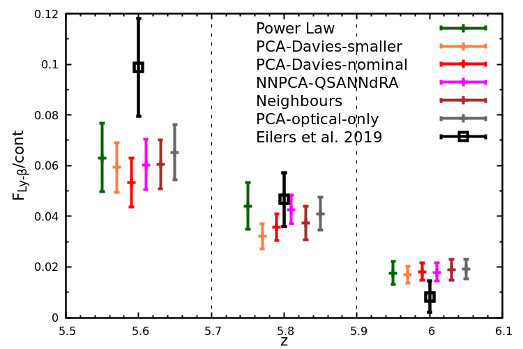
Figure 6: Mean transmitted Ly-$\beta$ flux along the sightlines of quasars at $z>5.7$. The coloured points correspond to predictions made from the five reconstruction methods which extend to $\lambda=972$Å, with bias corrections applied from testing on the $2.7<z<3.5$ eBOSS testing sample. The uncertainties account for both the $1\sigma$ uncertainties in reconstruction accuracy and observational errors. All techniques agree within $1.5\sigma$.

We note that since the power law’s bias is dominated by broad line residuals, its predictions are not immune to intrinsic quasar evolution with redshift. Indeed, if $z>5.7$ quasars have systematically weaker broad lines on both the red and blue side, the bias correction for the power-law fitting would be systematically over-estimated (see top left panel of Figure 4) or in other words, power-law extrapolations would be more correct on average at higher redshift. Perhaps surprisingly, we find that a PCA trained using only the $1220<\lambda(\text{\AA})<1450$ wavelength range succeeds in removing wavelength-dependent residuals coming from broad emission lines on the blue side (Figure 4, bottom right panel). The optical-only PCA has scatter $11.3\%$ and a small bias of $1.0\%$ over the testing sample. Theoretically, this implies the mean Ly-$\alpha$ transmission could be constrained without bias with a sufficient number of quasar spectra with appropriate SNR covering only observed optical wavelengths.

Over Ly-$\beta$ transmission, all methods have scatters of at least $16\%$ and systematic biases as large as $12\%$. Despite this, the recovered transmitted fluxes agree within $1.5\sigma$ for all methods after wavelength-dependent bias corrections were applied, and reconstruction uncertainties are taken into account (Figure 6). We find a shallower evolution of Ly-$\beta$ transmitted flux than reported in Eilers et al. (2019) with a discrepancy of $\sim 1.5\sigma$ at $5.5<z<5.7$. The Ly-$\beta$ continuum reconstruction method used in Eilers et al. (2019) stitches a PCA akin to PCA-Pâris-5 onto a quasar continuum from Shull et al. (2012), which is a complex procedure giving rise to unknown but likely significant bias and uncertainty. However, cosmic variance could also be the main driver of the observed discrepancies since the quasar samples of the two studies do not overlap.

5.1 Caveats

Three final caveats, which we do not address in this paper, relate to spectroscopic reduction residuals and selective wavelength masking. We outline those issues here and reflect on their consequences and possible mitigation measures.

The X-Shooter spectrograph has a data reduction process far more complex than eBOSS spectra, which involves an order of magnitude more stitchings of spectral orders in the observed IR and combination of the optical and IR spectrograph arms. Such residuals can bias all reconstruction methods, and perhaps impacting most strongly PCA methods as they aim to fit detailed red side features and least strongly neighbour-stacking methods which will implicitly marginalise over defects. Quantifying the effect of reduction errors could potentially be done by using large samples of quasars observed with both X-Shooter and the BOSS spectrograph, such as the XQ-100 sample (López et al., 2016).

Second, the rest-frame wavelengths affected by telluric absorption depend directly on the redshift of observed quasars. In this work, we masked the regions most severely affected by telluric absorption. All methods can implicitly adapt to missing data, but it may have a deeper effect on PCA methods. Since the number of PCA components is chosen to contain a fixed fraction of the observed variance in the training sample over a complete wavelength range, the same components might not have been retained if the same wavelength regions are missing. To quantify this effect, one could construct ‘tailored’ PCA decompositions by extracting the component vectors from a training sample in which the same wavelength regions are always masked.

Finally, the potential impact of quasar evolution with redshift on PCA reconstruction will be addressed in future work. Quasars with fewer neighbours will instinctively be less well captured by PCA reconstructions, and may occupy sparsely-populated regions of PCA component coefficients parameter space. Different definitions of quasar distance, and ‘tailored’ PCAs, may be ways to explore these effect in the future.

6 Conclusions

We have tested eight different quasar continuum reconstruction methods designed to measure Ly-$\alpha$ and Ly-$\beta$ transmission at $z>5.0$. We use a common testing sample consisting of $4579$ quasars at $2.7<z<3.5$ from the eBOSS catalogue. For three techniques which require training at low-$z$, we use a separate common training sample consisting of the same number of quasars. Our findings are:

• The continuum uncertainties arising from using power-law extrapolation are larger than has previously been assumed, at $+13.2\%/-13.1\%$ over Ly-$\alpha$ and $+19.9\%/-20.1\%$ over Ly-$\beta$ .

• Power-law reconstructions are also the most systematically biased due to the presence of broad emission lines on the blue side, by $\geq-9.58\%$ over Ly-$\alpha$ .

• PCA reconstructions trained on small samples and restricted to fewer components are also significantly biased, by $\geq+8.22\%$ over Ly-$\alpha$ .

• Using PCAs trained on large, cleaner samples and using improved blue-side recovery techniques, which we present there, it is possible to reduce the reconstruction uncertainty below $9\%$ over Ly-$\alpha$ and below $17\%$ over Ly-$\beta$ .

• The neural-network-mapped PCA, PCANN-QSANNdRA, performs nearly identically to newer ‘classical’ PCA methods for the $1\sigma$ scatter over the Ly-$\alpha$ and Ly-$\beta$ forests.

• Power-law reconstructions and small-sample PCAs create strong wavelength-dependent biases and scatter, of which newer methods are devoid.

We then assembled a sample of $19$ X-Shooter spectra of $z>5.7$ quasars with eBOSS-equivalent SNR $>7$ and present new results for the Ly-$\alpha$ and Ly-$\beta$ transmission at $z>5.0$, correcting for the wavelength-dependent biases we identified and accounting for continuum uncertainties. We conclude that:

• In the absence of rigorous tests at $z<5$, measurements of Ly-$\alpha$ and Ly-$\beta$ transmission at $z>5.0$ are liable to be biased by inaccurate continuum reconstructions by systematic errors in excess of statistical uncertainties.

• Using $z>5.7$ quasar spectra covering only observed optical wavelengths, it is still possible to constrain the intrinsic continuum within $+11.2\%/-11.3\%$ using optical-only PCA.

• Since the bias of power-law reconstructions is driven by broad emission lines on the blue side, we caution that they are not necessarily exempt from caveats related to intrinsic quasar evolution with redshift, whether due to a mismatch in intrinsic luminosity or more complex factors.

As more complex techniques will keep improving the quality of continuum predictions, it is important to keep testing these methods on well-controlled samples at low-$z$. The number of known quasars at $z>5.7$ and the quality of their spectra is quickly increasing, and reconstruction techniques for quasar continuum emission are likely to remain a crucial tool in the study of reionisation.

Data availability

The data underlying the testing and training samples, and further examples of the fitting methods, are available on the lead author’s website at http://www.sarahbosman.co.uk/research. The remainder of the data underlying this paper will be shared upon request to the corresponding author.

Appendix A Dependence of Power-Law reconstruction on wavelength range

Depending on quasar redshift, restricted ranges in wavelengths have to be used to fit power-law reconstructions at $z>5.7$ when only optical observations are available. We test the effect of varying the fitting range by repeating the procedure in Section 2.1 and changing that parameter only. The results are shown in Figure 7. Using a shorter range $1270<\lambda(\text{\AA})<1400$ does not produce any significant extra bias compared to the nominal range $1270<\lambda(\text{\AA})<1450$ we have used throughout the paper. The prediction scatter is increased by the shorter range by $\pm 2\%$ ($\pm 4\%$) at $1\sigma$ ($2\sigma$).

Shortening the range further to $1270<\lambda(\text{\AA})<1350$ does introduce an extra bias of $+16\%$ and dramatically inflates the scatter ($+49\%/-36\%$ at $1\sigma$). We suspect this is because the presence of the weak Si II $1303$Å and broad N V emission lines have a stronger effect on the best fit in the absence of the up-turn towards the broad Si IV $1396$ Å line. With a smaller fitting range, it is harder to separate the broad lines from the continuum and the fit becomes influenced by line ratios, resulting in increased bias and much increased scatter.

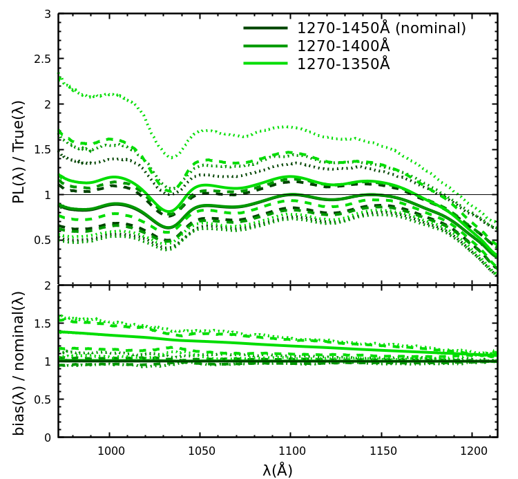
Figure 7: The effect of varying the wavelength range over which a power-law reconstruction is fit before extrapolating to the blue side. Dashed and dotted lines correspond to the contours encompassing $86\%$ (1$\sigma$) and $95\%$ ($2\sigma$) of the scatter, respectively.

Appendix B Effect of Proximity Zone Cut-Off on recovered $z>5$ transmission

A potentially important free parameter is the wavelength which marks the end of quasars’ effect on the surrounding IGM, $\lambda_{\text{prox}}$. In Bosman et al. (2018), we showed that stacks of quasar spectra at $z>5.7$ display no boost beyond $\lambda_{\text{prox}}=1176$Å and therefore adopted the value. We now wish to re-visit this measurement with accurate continuum reconstruction rather than the directly measured flux. According to the residuals in the power-law in Figure 4, the bias of the power-law fit at $\lambda>1176$Å at $z<3.5$ is not due only to a quasar’s proximity zone, but also to very broad and/or blue-shifted Ly-$\alpha$ emission lines. Indeed, the PCA-Davies series of PCAs show no bias until $\lambda\leq 1190$Å. Either way, it may be possible to recover IGM transmission to larger wavelengths than previously assumed. This is crucial, since the $5.9<z<6.1$ interval is only probed by a total $\int dz=3.888$ using $\lambda_{\text{prox}}=1176$Å. Furthermore, the stack of $z>6.1$ quasars in Bosman et al. (2018) shows much shorter proximity zones on average, only affecting the transmission at $\lambda\gtrsim 1190$Å.

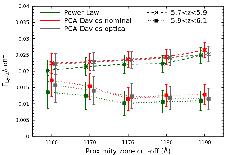
Figure 8: Values of mean transmitted Ly-$\alpha$ flux at $5.7<z<5.9$ and $5.9<z<6.1$, showing the effect of varying the proximity zone cut-off wavelength. We only show three methods, Power-Law, PCA-Davies-nominal and PCA-optical only for legibility. The transmitted flux increases as the cut-off is shifted to $\lambda_{\text{prox}}=1190$Å at $5.7<z<5.9$, reflecting the mean enhancement in quasars’ proximity zones. The effect is not seen at $5.9<z<6.1$, where proximity zones are shorter. The increase towards $\lambda_{\text{prox}}=1160$Å at $5.9<z<6.1$ is due to shifting of the mean redshift and reduced sample size.

We therefore repeat the procedure in Section 5 varying only $\lambda_{\text{prox}}$. The results are shown in Figure 8 for two redshift ranges, $5.7<z<5.9$ and $5.9<z<6.1$. We find an increase in transmission from $\lambda_{\text{prox}}=1176$Å to $\lambda_{\text{prox}}=1190$Å at $5.7<z<5.9$, but not $5.9<z<6.1$. This is in agreement with Bosman et al. (2018), and reflects the shorter sizes of proximity zones in $z>6.1$ quasars. In contrast, the transmission at $5.9<z<6.1$ shows an increase as the cut-off is made more stringent, $\lambda_{\text{prox}}=1160$Å. More stringent cut-offs severely reduce the total $\int dz$ probed by the sample from $\int dz=6.55$ with $\lambda_{\text{prox}}=1190$Å to $\int dz=2.40$ with $\lambda_{\text{prox}}=1160$Å, resulting in a large increase in uncertainty. Further, a stringent cut leads to a drift in the mean redshift of the transmission contributing to the bin, from $z_{\text{mean}}=5.986$ with $\lambda_{\text{prox}}=1190$Å to $z_{\text{mean}}=5.975$ with $\lambda_{\text{prox}}=1160$Å. Because the evolution with redshift is very fast, this leads to artificially inflated transmission.

We conclude the choice of $\lambda_{\text{prox}}$ can bias the measurement of mean transmission if it too loose but also if it is too stringent, when the sample size of quasars is small. Our choice of $\lambda=1176$Å sits at an acceptable compromise of the two effects described above. $\lambda=1180$Å might be a better choice as it increases the pathlength to $\int z=4.578$ at $5.9<z<6.1$, an increase of $18\%$. However, we stick with $\lambda=1176$Å due to the small increase in transmission towards $\lambda=1180$Å at $5.7<z<5.9$ and the existence of individual $z>5.7$ quasars with proximity zones existing almost to $\lambda=1180$Å (Carilli et al., 2010; Eilers et al., 2019; Bosman et al., 2020).

Appendix C Improved Continuum Fitting

Figure 9 shows our improved spline-fitting procedure over the Ly-$\alpha$ and Ly-$\beta$ forest. By explicitly removing strong absorbers, the fit is better able to recover the continuum with less bias over strong absorbers. This makes a difference at $z>3$, where our measured mean Ly-$\alpha$ flux is less biased than measured by Dall’Aglio et al. (2009), who used the original fitting procedure without the extra masking step.

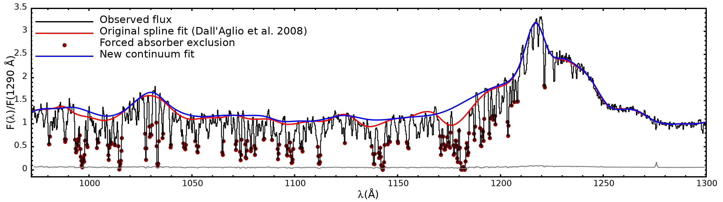
Figure 9: Showcase of the improved continuum fitting with exclusion of strong absorbers on the eBOSS quasar J113102.18+225910.5 at $z=3.373$, which is part of the testing sample.

Appendix D Effect of SNR on reconstructions

We investigate the effect of SNR on the continuum reconstruction by dividing the testing sample into the lowest-SNR half (SNR$<10.5$) and highest-SNR half (SNR$>10.5$). We focus on the two best-performing methods: PCA-Davies-nominal and PCANN-QSANNdRA. For PCA-Davies-nominal, the $1\sigma$ scatter increases slightly for the SNR$<10.5$ objects while the bias is slightly smaller. The nominal accuracy is $B_{\text{Ly}\alpha}=0.9\%-9.0/+8.8$, the high-SNR sample yields $B_{\text{Ly}\alpha}=1.0\%-8.4/+8.2$, and the low-SNR sample yields $B_{\text{Ly}\alpha}=0.8\%-9.5/+9.3$. The same trend is observed with PCANN-QSANNdRA: the $1\sigma$ uncertainties are increased by about $5\%$ for the lowest-SNR objects. In this case, the nominal accuracy is $B_{\text{Ly}\alpha}=0.3\%-9.2/+9.1$, the high-SNR sample yields $B_{\text{Ly}\alpha}=0.4\%-8.7/+8.6$, and the low-SNR sample yields $B_{\text{Ly}\alpha}=0.2\%-9.7/+9.6$.

The slightly increased uncertainties on low-SNR objects could be due to larger continuum fitting uncertainties on both the red and blue sides. This effect does not affect the relative performance of the methods, as PCA-Davies-nominal slightly outperforms PCANN-QSANNdRA on both the high- and low-SNR samples. Lower SNR does not introduce extra bias in the predictions, neither in the mean bias nor in the wavelength-dependent bias (Figure 10).

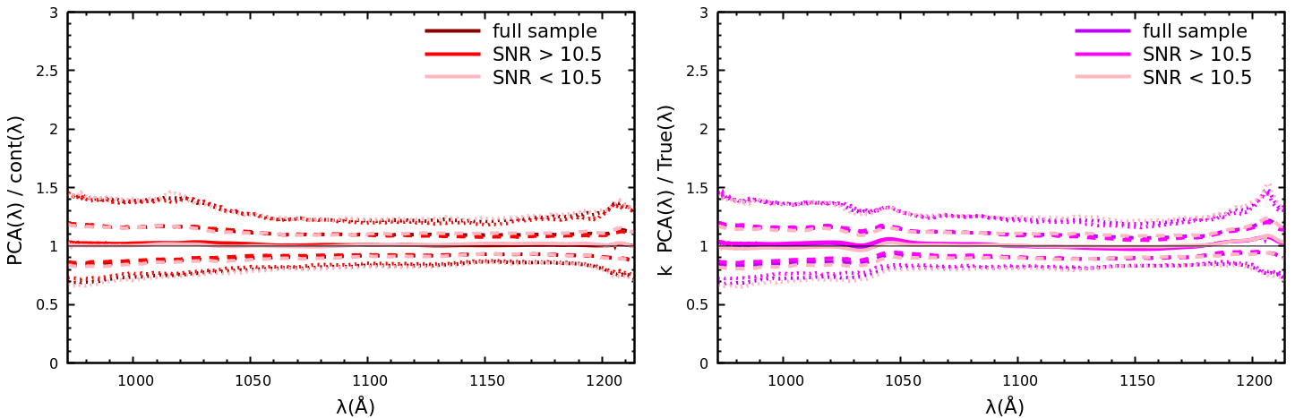
Figure 10: Wavelength-dependent bias and scatter as a function of object SNR, for PCA-Davies-nominal (left) and PCANN-QSANNdRA (right). Dashed and dotted lines correspond to the contours encompassing $86\%$ (1$\sigma$) and $95\%$ ($2\sigma$) of the scatter, respectively. Dividing the testing sample into the highest-SNR half (SNR$>10.5$) and lower-SNR half (SNR$<10.5$) does not reveal significant effects in the mean uncertainty and bias, nor in their wavelength-dependence.

Appendix E All fits

We show below all bias-corrected continuum reconstructions for our $19$ $z>5.7$ quasars (Figure E1). We always mask the region of strong telluric absorption at $13450<\lambda(\text{\AA})<14250$ since telluric correction introduces residuals which are not present in our testing sample. In low-SNR ($\lesssim 1$/pixel) X-Shooter spectra, it is difficult to correctly model the response curve of the last order in the optical arm and the first order in the IR arm. When stitching the arms introduced artifacts, or when unfortunately-located strong absorbers coincided with the overlap, we opt to mask the affected region entirely. In P239-07 and P359-06, we also mask strong associated absorbers near the Ly-$\alpha$ emission line.

We do not make predictions for the quasars’ Ly-$\alpha$ and Ly-$\beta$ proximity zones, shaded in grey. The correction due to mean IGM absorption at $z<3.5$ is different over the Ly-$\alpha$ and Ly-$\beta$ forest regions, leading to a discontinuity in the Ly-$\beta$ proximity zone. Most fits are satisfactory, with the methods showing scatter with respect to each other but no clear bias. Below are some notes on individual objects.

E.1 J0100+2802 and J1319+0950

The wavelength-dependent bias correction applied to the Power-Law fit reflect the average strength of blue-side broad emission lines at $z<3.5$. In J0100+2802 and J1319+0950, this mean prediction differs significantly from all other methods, indicating the quasars very likely have weaker O VI emission lines than average. Both also display weaker than average lines on the red side.

E.2 P056-16

Interestingly, in P056-16, all methods make very similar predictions except for the Power-Law. All techniques predict a break in the power law continuum, including stacks of Neighbours and PCA-optical only.

E.3 J0818+1722

The red side continuum of J0818+1722 is not well fit by any model. This is perhaps concerning since its stranger features (exceedingly broad and shifted C IV emission line, extended C III] and Si IV lines) are similar to what is seen in the $z=7.5$ quasar (Bañados et al., 2018). Modifying the redshift by up to $\delta z=0.1$, or using more complex convergence techniques to fit the PCA on the red side, did not alleviate this problem significantly. We plan to address this issue, and especially the dearth of low-$z$ analogues for certain $z>5.7$ quasars, in future work.

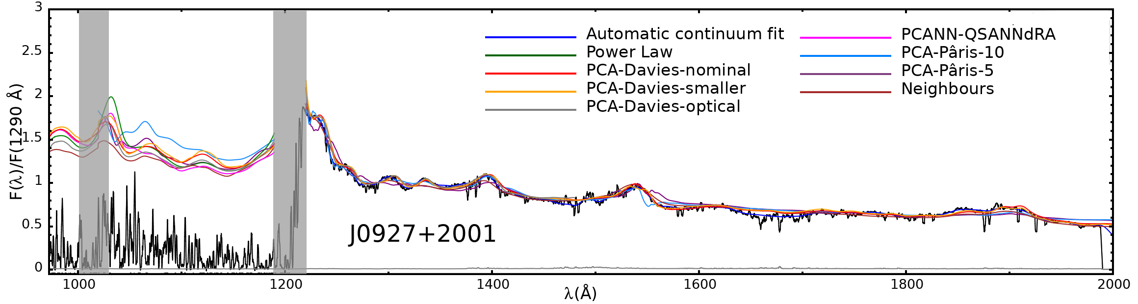
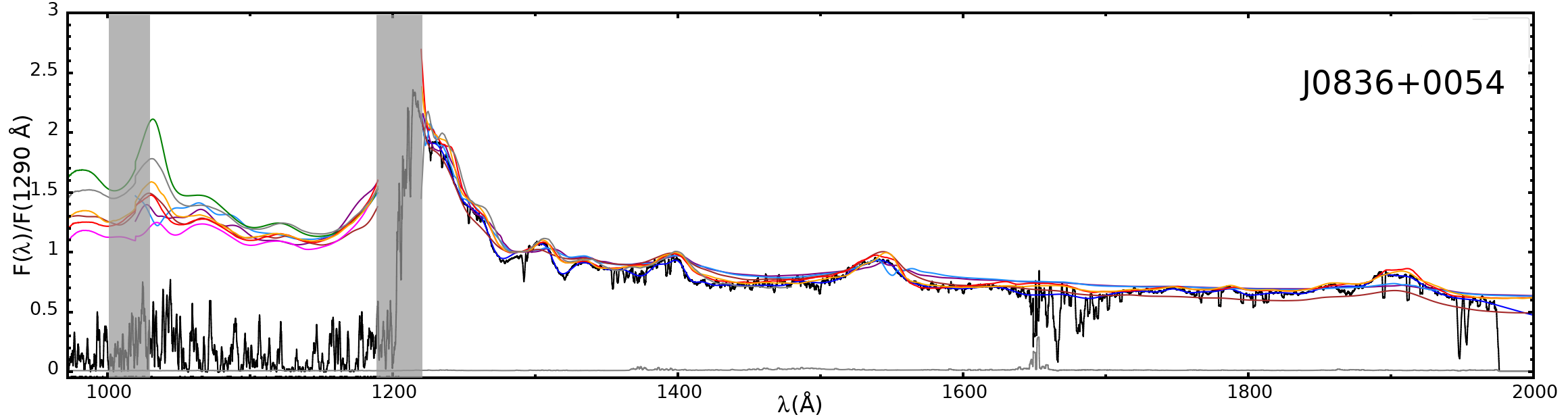
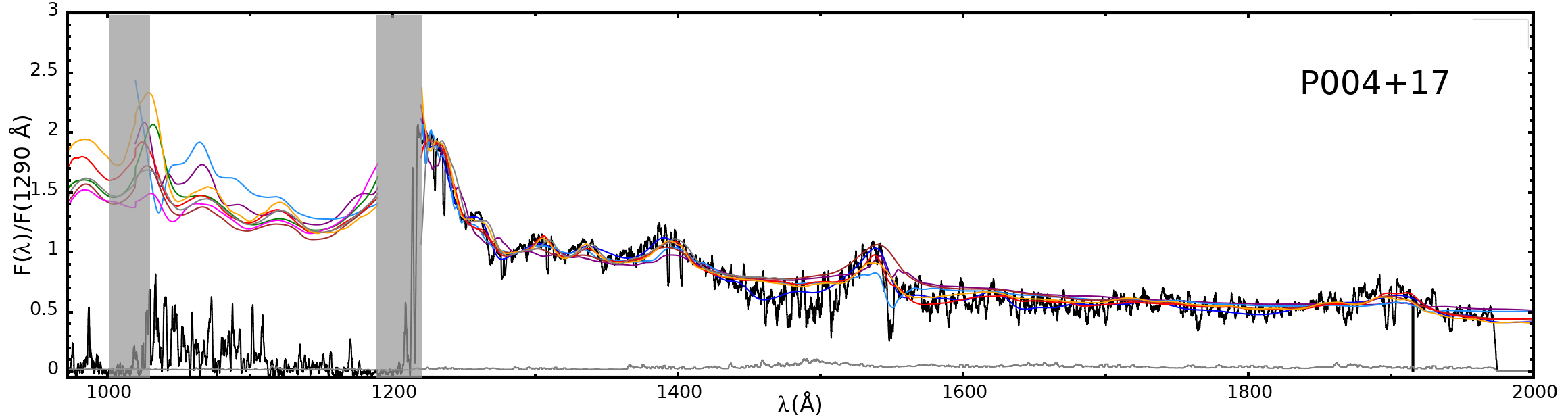
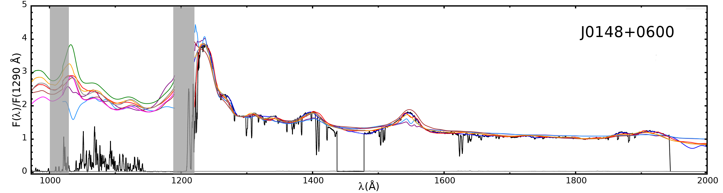
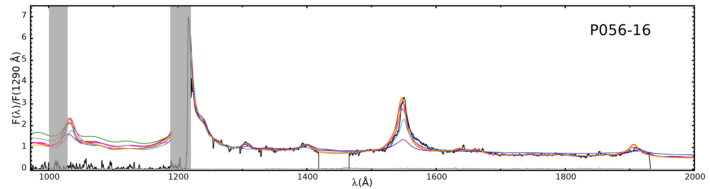
Figure 11: All continuum predictions for the $z>5.7$ quasars used to measure the mean Ly-$\alpha$ and Ly-$\beta$ opacity (including bias corrections). Reconstruction methods are indicated by different colours as shown in the legend. Notes on individual objects can be found in Appendix E.

References

- Astropy Collaboration et al. (2013) Astropy Collaboration et al., 2013, A&A, 558, A33
- Bañados et al. (2016) Bañados E., et al., 2016, ApJS, 227, 11
- Bañados et al. (2018) Bañados E., et al., 2018, Nature, 553, 473
- Balcells et al. (2010) Balcells M., et al., 2010, in Proc. SPIE. p. 77357G (arXiv:1008.0600), doi:10.1117/12.856947
- Baldwin (1977) Baldwin J. A., 1977, ApJ, 214, 679
- Becker & Bolton (2013) Becker G. D., Bolton J. S., 2013, MNRAS, 436, 1023
- Becker et al. (2015) Becker G. D., Bolton J. S., Madau P., Pettini M., Ryan-Weber E. V., Venemans B. P., 2015, MNRAS, 447, 3402
- Becker et al. (2018) Becker G. D., Davies F. B., Furlanetto S. R., Malkan M. A., Boera E., Douglass C., 2018, ApJ, 863, 92
- Boera et al. (2019) Boera E., Becker G. D., Bolton J. S., Nasir F., 2019, ApJ, 872, 101
- Bosman & Becker (2015) Bosman S. E. I., Becker G. D., 2015, MNRAS, 452, 1105
- Bosman et al. (2018) Bosman S. E. I., Fan X., Jiang L., Reed S., Matsuoka Y., Becker G., Haehnelt M., 2018, MNRAS, 479, 1055
- Bosman et al. (2020) Bosman S. E. I., Kakiichi K., Meyer R. A., Gronke M., Laporte N., Ellis R. S., 2020, ApJ, 896, 49
- Brandt & LSST Active Galaxies Science Collaboration (2007) Brandt N., LSST Active Galaxies Science Collaboration 2007, in American Astronomical Society Meeting Abstracts. p. 137.09
- Carilli et al. (2010) Carilli C. L., et al., 2010, ApJ, 714, 834
- Carswell et al. (1982) Carswell R. F., Whelan J. A. J., Smith M. G., Boksenberg A., Tytler D., 1982, MNRAS, 198, 91
- Chardin et al. (2015) Chardin J., Haehnelt M. G., Aubert D., Puchwein E., 2015, MNRAS, 453, 2943
- Chardin et al. (2018) Chardin J., Haehnelt M. G., Bosman S. E. I., Puchwein E., 2018, MNRAS, 473, 765
- Chehade et al. (2018) Chehade B., et al., 2018, MNRAS, 478, 1649
- Choudhury et al. (2021) Choudhury T. R., Paranjape A., Bosman S. E. I., 2021, MNRAS, 501, 5782
- Coatman et al. (2016) Coatman L., Hewett P. C., Banerji M., Richards G. T., 2016, MNRAS, 461, 647
- Cool et al. (2006) Cool R. J., et al., 2006, AJ, 132, 823
- Crighton et al. (2015) Crighton N. H. M., et al., 2015, MNRAS, 452, 217
- D’Aloisio et al. (2015) D’Aloisio A., McQuinn M., Trac H., 2015, ApJ, 813, L38
- D’Aloisio et al. (2018) D’Aloisio A., McQuinn M., Davies F. B., Furlanetto S. R., 2018, MNRAS, 473, 560
- DESI Collaboration et al. (2016) DESI Collaboration et al., 2016, arXiv e-prints, p. arXiv:1611.00036
- Dall’Aglio et al. (2008) Dall’Aglio A., Wisotzki L., Worseck G., 2008, A&A, 491, 465
- Dall’Aglio et al. (2009) Dall’Aglio A., Wisotzki L., Worseck G., 2009, arXiv e-prints, p. arXiv:0906.1484
- Davies & Furlanetto (2016) Davies F. B., Furlanetto S. R., 2016, MNRAS, 460, 1328
- Davies et al. (2018a) Davies F. B., Becker G. D., Furlanetto S. R., 2018a, ApJ, 860, 155
- Davies et al. (2018b) Davies F. B., et al., 2018b, ApJ, 864, 142
- Davies et al. (2018c) Davies F. B., et al., 2018c, ApJ, 864, 143
- Dawson et al. (2013) Dawson K. S., et al., 2013, AJ, 145, 10
- Dawson et al. (2016) Dawson K. S., et al., 2016, AJ, 151, 44
- Decarli et al. (2017) Decarli R., et al., 2017, Nature, 545, 457
- Dijkstra et al. (2016) Dijkstra M., Gronke M., Venkatesan A., 2016, ApJ, 828, 71
- Eilers et al. (2017) Eilers A.-C., Davies F. B., Hennawi J. F., Prochaska J. X., Lukić Z., Mazzucchelli C., 2017, ApJ, 840, 24
- Eilers et al. (2018) Eilers A.-C., Davies F. B., Hennawi J. F., 2018, ApJ, 864, 53
- Eilers et al. (2019) Eilers A.-C., Hennawi J. F., Davies F. B., Oñorbe J., 2019, ApJ, 881, 23
- Eilers et al. (2020) Eilers A.-C., et al., 2020, arXiv e-prints, p. arXiv:2002.01811
- Fan et al. (2000) Fan X., et al., 2000, AJ, 120, 1167
- Fan et al. (2001) Fan X., et al., 2001, AJ, 122, 2833
- Fan et al. (2002) Fan X., Narayanan V. K., Strauss M. A., White R. L., Becker R. H., Pentericci L., Rix H.-W., 2002, AJ, 123, 1247
- Fan et al. (2006) Fan X., et al., 2006, AJ, 132, 117
- Fathivavsari (2020) Fathivavsari H., 2020, arXiv e-prints, p. arXiv:2006.05124
- Faucher-Giguère et al. (2008) Faucher-Giguère C.-A., Prochaska J. X., Lidz A., Hernquist L., Zaldarriaga M., 2008, ApJ, 681, 831
- Francis et al. (1992) Francis P. J., Hewett P. C., Foltz C. B., Chaffee F. H., 1992, ApJ, 398, 476
- Fukugita et al. (1996) Fukugita M., Ichikawa T., Gunn J. E., Doi M., Shimasaku K., Schneider D. P., 1996, AJ, 111, 1748
- Gaikwad et al. (2020) Gaikwad P., et al., 2020, MNRAS, 494, 5091
- Gallerani et al. (2006) Gallerani S., Choudhury T. R., Ferrara A., 2006, MNRAS, 370, 1401
- Gnedin et al. (2017) Gnedin N. Y., Becker G. D., Fan X., 2017, ApJ, 841, 26
- Greig et al. (2017) Greig B., Mesinger A., Haiman Z., Simcoe R. A., 2017, MNRAS, 466, 4239
- Gunn & Peterson (1965) Gunn J. E., Peterson B. A., 1965, ApJ, 142, 1633
- Hewett & Wild (2010) Hewett P. C., Wild V., 2010, MNRAS, 405, 2302
- Hunter (2007) Hunter J. D., 2007, Computing in Science Engineering, 9, 90
- Ivezić et al. (2019) Ivezić Ž., et al., 2019, ApJ, 873, 111
- Jiang et al. (2015) Jiang L., McGreer I. D., Fan X., Bian F., Cai Z., Clément B., Wang R., Fan Z., 2015, AJ, 149, 188
- Kakiichi et al. (2018) Kakiichi K., et al., 2018, MNRAS, 479, 43
- Kashino et al. (2020) Kashino D., Lilly S. J., Shibuya T., Ouchi M., Kashikawa N., 2020, ApJ, 888, 6
- Keating et al. (2020) Keating L. C., Weinberger L. H., Kulkarni G., Haehnelt M. G., Chardin J., Aubert D., 2020, MNRAS, 491, 1736
- Krolik & Kallman (1988) Krolik J. H., Kallman T. R., 1988, ApJ, 324, 714
- Kulkarni et al. (2019) Kulkarni G., Keating L. C., Haehnelt M. G., Bosman S. E. I., Puchwein E., Chardin J., Aubert D., 2019, MNRAS, 485, L24
- Lee et al. (2012) Lee K.-G., Suzuki N., Spergel D. N., 2012, AJ, 143, 51
- Lee et al. (2015) Lee K.-G., et al., 2015, ApJ, 799, 196
- Lidz et al. (2006) Lidz A., Oh S. P., Furlanetto S. R., 2006, ApJ, 639, L47
- Liu & Bordoloi (2021) Liu B., Bordoloi R., 2021, MNRAS, 502, 3510
- López et al. (2016) López S., et al., 2016, A&A, 594, A91
- Madau & Haardt (2015) Madau P., Haardt F., 2015, ApJ, 813, L8
- Mao et al. (2008) Mao Y., Tegmark M., McQuinn M., Zaldarriaga M., Zahn O., 2008, Phys. Rev. D, 78, 023529
- Margala et al. (2016) Margala D., Kirkby D., Dawson K., Bailey S., Blanton M., Schneider D. P., 2016, ApJ, 831, 157
- Mazzucchelli et al. (2017) Mazzucchelli C., et al., 2017, ApJ, 849, 91
- McDonald et al. (2005) McDonald P., Seljak U., Cen R., Bode P., Ostriker J. P., 2005, MNRAS, 360, 1471
- McDonald et al. (2006) McDonald P., et al., 2006, ApJS, 163, 80
- McGreer et al. (2011) McGreer I. D., Mesinger A., Fan X., 2011, MNRAS, 415, 3237
- McGreer et al. (2015) McGreer I. D., Mesinger A., D’Odorico V., 2015, MNRAS, 447, 499
- Meiksin (2020) Meiksin A., 2020, MNRAS, 491, 4884
- Meyer et al. (2019a) Meyer R. A., Bosman S. E. I., Kakiichi K., Ellis R. S., 2019a, MNRAS, 483, 19
- Meyer et al. (2019b) Meyer R. A., Bosman S. E. I., Ellis R. S., 2019b, MNRAS, 487, 3305
- Meyer et al. (2020) Meyer R. A., et al., 2020, MNRAS, 494, 1560
- Mortlock et al. (2009) Mortlock D. J., et al., 2009, A&A, 505, 97
- Mortlock et al. (2011) Mortlock D. J., et al., 2011, Nature, 474, 616
- Nasir & D’Aloisio (2020) Nasir F., D’Aloisio A., 2020, MNRAS, 494, 3080
- Nasir et al. (2016) Nasir F., Bolton J. S., Becker G. D., 2016, MNRAS, 463, 2335
- Oñorbe et al. (2017) Oñorbe J., Hennawi J. F., Lukić Z., Walther M., 2017, ApJ, 847, 63
- Oh & Furlanetto (2005) Oh S. P., Furlanetto S. R., 2005, ApJ, 620, L9
- Pâris et al. (2011) Pâris I., et al., 2011, A&A, 530, A50
- Pâris et al. (2017) Pâris I., et al., 2017, A&A, 597, A79
- Pâris et al. (2018) Pâris I., et al., 2018, A&A, 613, A51
- Pedregosa et al. (2011) Pedregosa F., et al., 2011, Journal of Machine Learning Research, 12, 2825
- Perez & Granger (2007) Perez F., Granger B. E., 2007, Computing in Science Engineering, 9, 21
- Pérez-Ràfols et al. (2018) Pérez-Ràfols I., Miralda-Escudé J., Arinyo-i-Prats A., Font-Ribera A., Mas-Ribas L., 2018, MNRAS, 480, 4702
- Planck Collaboration et al. (2018) Planck Collaboration et al., 2018, arXiv e-prints, p. arXiv:1807.06209
- Planck Collaboration et al. (2020) Planck Collaboration et al., 2020, A&A, 641, A6
- Price-Whelan et al. (2018) Price-Whelan A. M., et al., 2018, AJ, 156, 123
- Prochaska (2017) Prochaska J. X., 2017, Astronomy and Computing, 19, 27
- Prochaska et al. (2009) Prochaska J. X., Worseck G., O’Meara J. M., 2009, ApJ, 705, L113
- Prochaska et al. (2019) Prochaska J. X., et al., 2019, pypeit/PypeIt: Releasing for DOI, doi:10.5281/zenodo.3506873
- Prochaska et al. (2020) Prochaska J., et al., 2020, The Journal of Open Source Software, 5, 2308
- Rafelski et al. (2014) Rafelski M., Neeleman M., Fumagalli M., Wolfe A. M., Prochaska J. X., 2014, ApJ, 782, L29
- Rankine et al. (2020) Rankine A. L., Hewett P. C., Banerji M., Richards G. T., 2020, MNRAS, 492, 4553
- Reed et al. (2017) Reed S. L., et al., 2017, MNRAS, 468, 4702
- Richards et al. (2001) Richards G. T., et al., 2001, AJ, 121, 2308
- Richards et al. (2011a) Richards G. T., et al., 2011a, AJ, 141, 167
- Richards et al. (2011b) Richards J. W., et al., 2011b, ApJ, 733, 10
- Robertson et al. (2013) Robertson B. E., et al., 2013, ApJ, 768, 71
- Robertson et al. (2015) Robertson B. E., Ellis R. S., Furlanetto S. R., Dunlop J. S., 2015, ApJ, 802, L19
- Scott et al. (2004) Scott J. E., Kriss G. A., Brotherton M., Green R. F., Hutchings J., Shull J. M., Zheng W., 2004, ApJ, 615, 135
- Sheinis et al. (2002) Sheinis A. I., Bolte M., Epps H. W., Kibrick R. I., Miller J. S., Radovan M. V., Bigelow B. C., Sutin B. M., 2002, PASP, 114, 851
- Shen et al. (2008) Shen Y., Greene J. E., Strauss M. A., Richards G. T., Schneider D. P., 2008, ApJ, 680, 169
- Shen et al. (2019) Shen Y., et al., 2019, ApJ, 873, 35
- Shull et al. (2012) Shull J. M., Stevans M., Danforth C. W., 2012, ApJ, 752, 162
- Simcoe et al. (2011) Simcoe R. A., et al., 2011, ApJ, 743, 21
- Smee et al. (2013) Smee S. A., et al., 2013, AJ, 146, 32
- Songaila (2004) Songaila A., 2004, AJ, 127, 2598
- Songaila & Cowie (2002) Songaila A., Cowie L. L., 2002, AJ, 123, 2183
- Stark (2016) Stark D. P., 2016, ARA&A, 54, 761
- Suzuki (2006) Suzuki N., 2006, ApJS, 163, 110
- Suzuki et al. (2005) Suzuki N., Tytler D., Kirkman D., O’Meara J. M., Lubin D., 2005, ApJ, 618, 592
- Telfer et al. (2002) Telfer R. C., Zheng W., Kriss G. A., Davidsen A. F., 2002, ApJ, 565, 773
- Trott & Pober (2019) Trott C. M., Pober J. C., 2019, arXiv e-prints, p. arXiv:1909.12491
- Vanden Berk et al. (2001) Vanden Berk D. E., et al., 2001, AJ, 122, 549
- Vernet et al. (2011) Vernet J., et al., 2011, A&A, 536, A105
- Virtanen et al. (2019) Virtanen P., et al., 2019, scipy/scipy: SciPy 1.2.1, doi:10.5281/zenodo.2560881
- Wang et al. (2016) Wang F., et al., 2016, ApJ, 819, 24
- Wang et al. (2020) Wang F., et al., 2020, arXiv e-prints, p. arXiv:2004.10877
- White et al. (2003) White R. L., Becker R. H., Fan X., Strauss M. A., 2003, AJ, 126, 1
- Willott et al. (2007) Willott C. J., et al., 2007, AJ, 134, 2435
- Willott et al. (2010) Willott C. J., et al., 2010, AJ, 139, 906
- Willott et al. (2015) Willott C. J., Bergeron J., Omont A., 2015, ApJ, 801, 123
- Wolfe et al. (2005) Wolfe A. M., Gawiser E., Prochaska J. X., 2005, ARA&A, 43, 861
- Worseck et al. (2019) Worseck G., Davies F. B., Hennawi J. F., Prochaska J. X., 2019, ApJ, 875, 111
- Wu et al. (2015) Wu X.-B., et al., 2015, Nature, 518, 512
- Yip et al. (2004) Yip C. W., et al., 2004, AJ, 128, 2603
- Young et al. (1979) Young P. J., Sargent W. L. W., Boksenberg A., Carswell R. F., Whelan J. A. J., 1979, ApJ, 229, 891
- Ďurovčíková et al. (2020) Ďurovčíková D., Katz H., Bosman S. E. I., Davies F. B., Devriendt J., Slyz A., 2020, MNRAS,
- van der Walt et al. (2011) van der Walt S., Colbert S. C., Varoquaux G., 2011, Computing in Science Engineering, 13, 22