Imperfections and corrections
Abstract
The measurement and correction of optics parameters has been a major concern since the advent of strong focusing synchrotron accelerators. A review of typical imperfections in accelerator optics together with measurement and correction algorithms is given with emphasis on numerical implementations. Python examples are shown using existing libraries when possible.
0.1 Introduction
Imperfections in accelerator lattices cause beam parameters to deviate from design. An illustration is shown in Fig. 1, where ideal and perturbed functions are shown. The perturbation assumed is simply a 10% gradient error in the 8th defocusing quadrupole. This causes large relative deviations in functions of up to 500% with respect to the design value. This is usually called -beating and represented by .
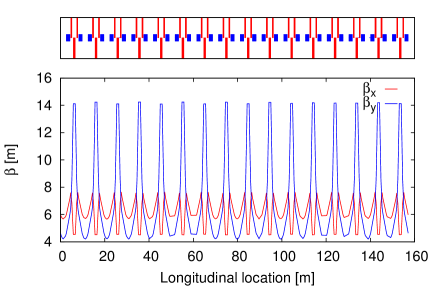
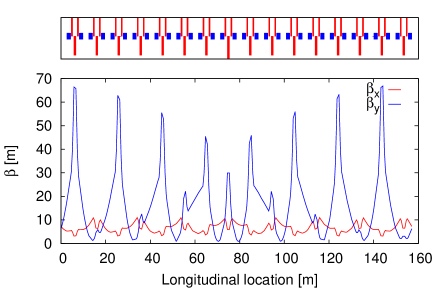
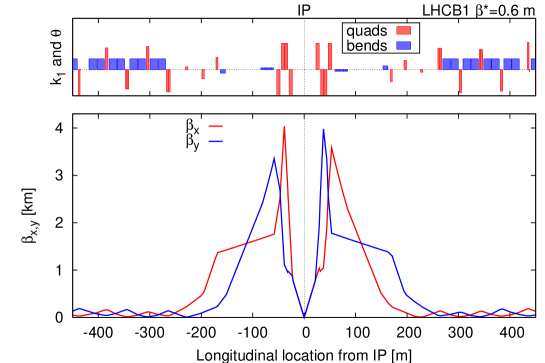
Perturbations from field imperfections and misalignments became a concern along with the conception of the strong focusing theory in 1957 [1]. However, the assumed approach was to specify design tolerances that would not impact machine performance. For example in [1] it is envisaged that with 1% rms gradient errors any particular machine would be unlikely to have more than 8% peak -beating. At that time they did not foresee the great developments in optics that would push functions to very large values, e.g., in the vicinity of collision points of collider accelerators. The LHC Interaction Region (IR) optics is shown in Fig. 2 as an illustration of optics designs reaching functions of several km.
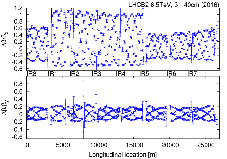
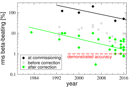
Modern accelerators have experienced -beating values above 100% [2, 3, 4] in the initial commissioning phases. Figure 3 shows the initial -beating measured in the LHC commissioning in 2016 with a peak value of 120%. The optics errors need to be corrected below specified tolerances for safe and efficient operation. The development of the optics measurement and correction techniques is illustrated by the evolution of the -beating over time for many circular accelerators, see Fig. 4.
The techniques to measure and correct optics are described in the following with special emphasis on analysis algorithms and computing aspects. Section 0.2 gives the requirements to run the code examples below. Section 0.3 describes the most important imperfections present in accelerator lattices. Section 0.4 describes the key particle dynamics used in optics measurements. Section 0.5 reports on the most used measurement techniques and data analysis techniques. Section 0.6 is an interlude devoted to the Farey sequences and how they can be used to describe the resonance diagram. Section 0.7 reports on optics correction techniques.
0.2 Requirements for code examples
Code examples below require Python. The freely available and open source operative system Ubuntu has Python by default. The required plotting and numerical libraries can be installed with, e.g., the following shell command:
Alternatively it is also possible to install Anaconda which is a very complete Python free distribution with the required scientific packages.
0.3 Accelerator elements and their imperfections
0.3.1 Dipole
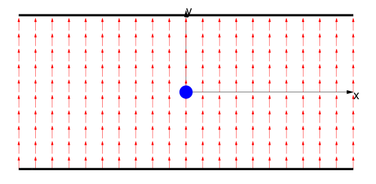
The simplest magnetic element in an accelerator is the dipole, which provides an homogeneous field as shown in Fig. 5.
The dipole features two main imperfections: a strength error and a tilt of the field around the beam axis. The tilt error is illustrated in Fig. 6 and can be interpreted as another dipole with a field orthogonal to the ideal dipole.
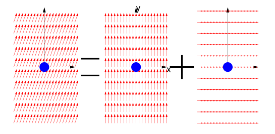
Therefore dipole errors are seen as unwanted angular deflections in both transverse planes that distort the reference trajectories into new closed orbits. Assuming to be unwanted angular deflections the closed orbit is given by
| (1) |
where denotes the longitudinal location around the ring, is the tune and is the betatron phase advance. The denominator makes closed orbit to diverge at the integer resonance . The effect of longitudinal misalignments is briefly described in Section 0.3.4. Another source of orbit errors is offset quadrupoles which is described in the following section.
0.3.2 Quadrupole
Figure 7 shows the magnetic and the force fields inside a quadrupole. An offset quadrupole is seen as the superposition of a centered quadrupole plus a dipolar field, as shown in Fig. 8, hence introducing orbit deviations.
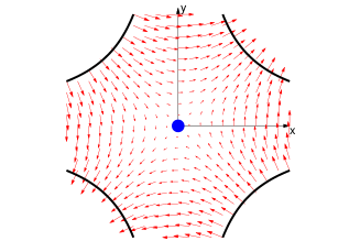

If the quadrupole in a lattice has a gradient error of it introduces horizontal and vertical tune deviations given by
| (2) |
where is the length of the quadrupole and stands for the average function in the quadrupole. At the same time the gradient error also introduces -beating. In presence of many quadrupolar errors the -beating can be expressed as
| (3) |
where the positive sign stands for the horizontal plane, and negative for the vertical. The denominator makes the -beating diverge at the integer and half integer resonances, . Betatron phase deviations between two locations in the accelerator, and , can be computed using the fundamental relation , yielding
| (4) |
More explicit first and higher order expansions of the phase beating can be found in [6, 7, 8]. Resonance driving terms, , appear in the expansion of the Hamiltonian and characterize the strength of resonances, , with any integer. are connected to the generating function resonance driving terms via the following relation,
| (5) |
where the denominator reveals the resonant behaviour. One way to explore higher order perturbations in the -beating is via the the generating function resonance driving term (in the horizontal plane), that is defined as
| (6) |
where is cycled so to start from 0 at . The -beating can be expressed as function of via the following equation [8],
| (7) |
where is the phase of . Similar equations hold for the vertical plane with .
Figure 9 shows a sketch of the variation of function along a quadrupole, displaying the the average function as and the at the edges as . An approximation of is given in [9] as
| (8) |
Exact equations for depend also on the quadrupole strength as shown in [10, 11].
A tilted quadrupole is seen as a normal quadrupole plus another quadrupole tilted by 45∘, which is called a skew quadrupole, see Fig. 10. The magnetic and force fields of a skew quadrupole are shown in Fig. 11.
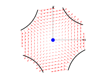
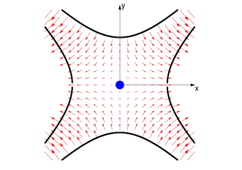
As shown in Fig. 11 particles displaced horizontally in a skew quadrupole receive a vertical force. This causes the particle motion to couple between the horizontal and vertical planes. While the uncoupled betatron motion of the particle position at turn and location is simply expressed as
| (9) |
with being the horizontal single particle emittance and the phase at and , the coupled motion in presence of skew quadrupolar fields can be approximated as [12, 13]
where stands for the real part of , and and are the sum and difference generating function resonance driving terms given by
| (12) |
where represents the skew quadrupole gradient in the machine. drives the difference resonance and drives the sum resonance , for any and .
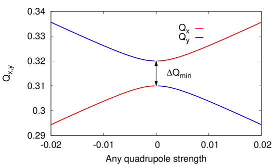
Another important feature of coupled motion is the appearance of a stopband around the difference resonance , . This implies that the fractional tunes cannot get closer than , the closest tune approach, given by [14]
| (13) |
where represents the skew quadrupolar gradients around the ring, is the machine radius and are the fractional tunes. can also be computed from around the ring by [15, 16]
| (14) |
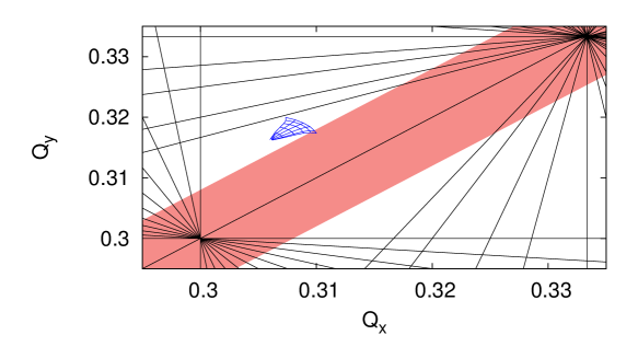
where represents the ring average of . As an illustration, a hypothetical large coupling stopband (in red) would limit the tune space available for the LHC beam-beam tune footprint as shown in Fig. 13.
0.3.3 Sextupole
Figure 14 shows the field and force fields in a sextupole.
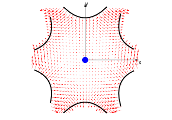
The equations describing the horizontal and vertical forces in a sextupole are given by
| (15) |
where is the integrated sextupolar gradient. Sextupoles are needed in accelerators to compensate chromaticity (), that describes the dependence of the tune with the relative energy deviation of the particle: , with . An offset sextupole is seen as a centered sextupole together with an offset quadrupole, see Fig. 15. Horizontal offsets in sextupoles generate normal quadrupole perturbations while vertical offsets generate skew quadrupolar fields.

0.3.4 Longitudinal misalignments
Longitudinal misalignments can be approximated as thin perturbations at both ends of the ideal magnet with opposite signs as shown in Fig. 16. For a longitudinal misalignment by of an element of strength the thin perturbations have integrated strengths of . Tolerances are generally larger for longitudinal misalignments as there is usually a partial compensation of the perturbations generated at both ends thanks to the opposite signs.

0.4 Phase-space and turn-by-turn motion
0.4.1 The transverse phase-space
At any location of the accelerator the turn-by-turn uncoupled motion is represented by the position of the particle and its angle with respect to the longitudinal direction, i.e. , which are parametrized as follows
| (16) |
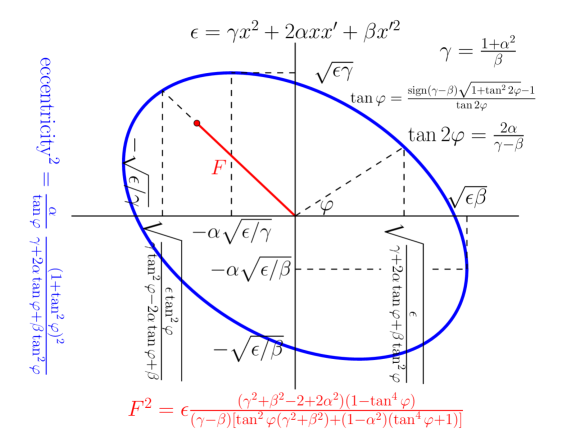
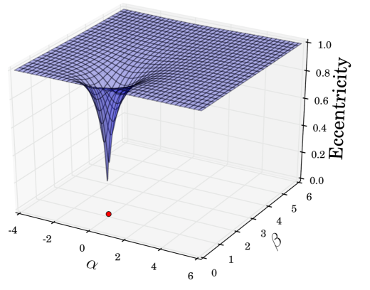
where . The particle trajectory stays within an ellipse in the phase-space . This trajectory is shown in Fig. 17 along with several relevant parameters of the motion and the ellipse, as the angle of the principal direction of the ellipse , the coordinates of the intersections of the ellipse and the axes, the largest excursions in and , the eccentricity of the ellipse and its focal length . The eccentricity of a conic section is a non-negative real number that uniquely characterizes its shape. More formally two conic sections are similar if and only if they have the same eccentricity. One can think of the eccentricity as a measure of how much a conic section deviates from being circular. In particular the eccentricity of a circle is zero and the eccentricity of an ellipse is greater than zero and smaller than 1. Figure 18 shows the eccentricity of the betatronic ellipse versus and . It is interesting to note that the motion is a circle only for and .
Expressing Eqs. (16) in matrix form illustrates the transformation that takes a circular motion into the elliptical one as follows,
| (17) | |||||
The circular motion is preferred in many studies for its simplicity and it is referred to as Normal form or Floquet Normal form.
0.4.2 Computing , and
When performing computer simulations of particles traveling in an accelerator subject to lattice imperfections or other electrodynamics interactions we have access to the turn-by-turn coordinates and we want to study how the different phenomena perturb the phase-space ellipse. Evaluating , and is possible by computing the singular value decomposition of the matrix composed of the and coordinates for turns,
| (18) |
where and are unitary matrices and is diagonal with non-negative real numbers on the diagonal. The diagonal entries of are known as singular values. The columns of and the columns of are called the left-singular vectors and right-singular vectors respectively. The left-singular vectors are a set of orthonormal vectors and similarly for the right-singular vectors.
represents the turn-by-turn motion in a circle (like a Normal form) in an arbitrary phase origin. Therefore, there must be a rotation than can be inserted in the singular value decomposition as
| (19) |
such that corresponds to the Floquet Normal Form, which has as main characteristic that the (1,2) element in the transformation of Eq. (17) is zero. We have to solve the following equation,
| (20) |
where is determined to make zero the element (1,2) of . The normalization factor is related to the single particle emittance as follows,
| (21) |
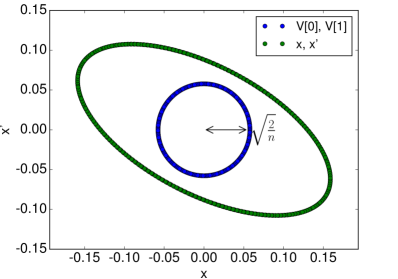
where is the number of turns. The following Python code implements the function that computes , and from turn-by-turn data together with an illustrative example. Figure 19 shows the turn-by-turn data used in the code example together with the first two right-singular vectors of .
A first version of this code was developed in [17].
0.4.3 Excitation techniques
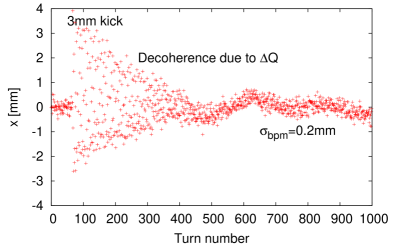
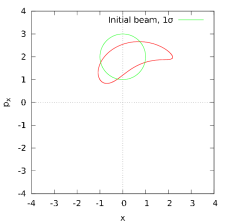
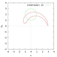
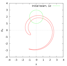
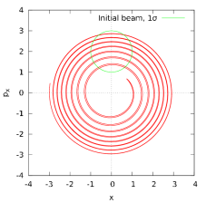
In real accelerators Beam Position Monitors (BPMs) measure transverse beam centroid position turn-by-turn, while the angle of the trajectory is not easily accessible. Betatron motion is usually excited via applying a single kick or via a resonant excitation The single kick technique has the limitation that due to non-linearities not all the particles in the bunch oscillate with the same tune the motion eventually decoheres. The measured turn-by-turn data following a single kick is illustrated in Figure 20. The evolution of the decoherence process is illustrated in Figure 21, where the initial 1 envelope after the kick is shown in green and the deformation of this envelope with time emerges from the larger tune values for particles with larger amplitude (amplitude detuning is typically generated by sextupoles, octupoles or the beam-beam interaction). The decoherence of the beam limits the number of turns available for data analysis and therefore limits the accuracy of beam-based optics measurements.
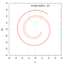
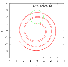
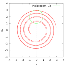
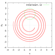
To avoid the limitation from decoherence it is possible to drive betatron oscillations with an AC dipole with a frequency close to the tune. Furthermore this forced oscillation can be ramped up and down adiabatically without causing emittance growth. The AC dipole cycle is illustrated in Fig. 22.

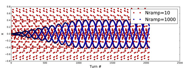
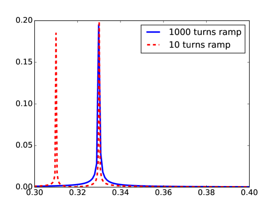
The adiabaticity of the ramping process of an AC dipole [18] can be easily simulated with the following code, which is used to produce the plot in Fig. 23 that compares the particle turn-by-turn motion for two AC dipole ramp-up lengths, 10 and 1000 turns, showing a lack of adiabaticity for the 10 turn ramp. The lack of adiabaticity implies energy transfer to the natural betatron motion with tune equal 0.31 as shown in the spectral components of particle motion in Fig. 24 as computed in the following example code.
0.5 Measurement techniques and data analysis
0.5.1 Cleaning experimental BPM data
The BPM turn-by-turn data is fundamental to measure optics parameters around the accelerator. Betatron oscillations represent highly correlated signals among BPMs. This feature can be used to reduce the BPM noise by discarding the signals with low correlation levels. SVD is used for this purpose. Imagine is the BPM matrix containing turn-by-turn data for all BPMs and his SVD is given by,
| (22) |
If , then we can neglect by making and reconstruct loosing a negligible amount of information. Denoting the reconstructed matrix as , it is given by the following equation,
| (23) |
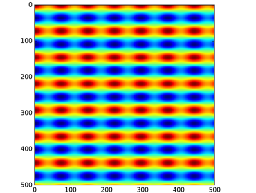
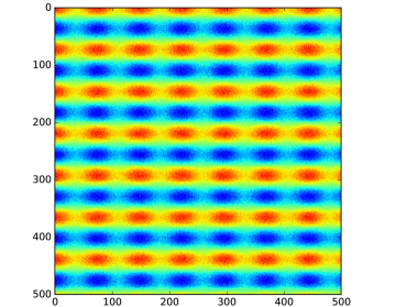
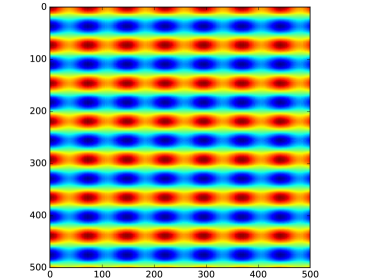
This technique is illustrated with the following Python code and in Fig. 25. In the code turn-by-turn data is simulated with very low tunes to produce pictures that can be easily visualized. Random Gaussian noise is added to mimic BPM noise with signal-to-noise ratio varying between 1:0.2 and 2:0.2. The SVD reconstruction is performed by keeping only the two largest singular values. The process is illustrated in Fig. 25 showing the 3 matrices in color code. It is impressive that the reconstructed matrix looks identical to the ideal one before adding the noise. Actually this technique is equally used to denoise digital pictures.
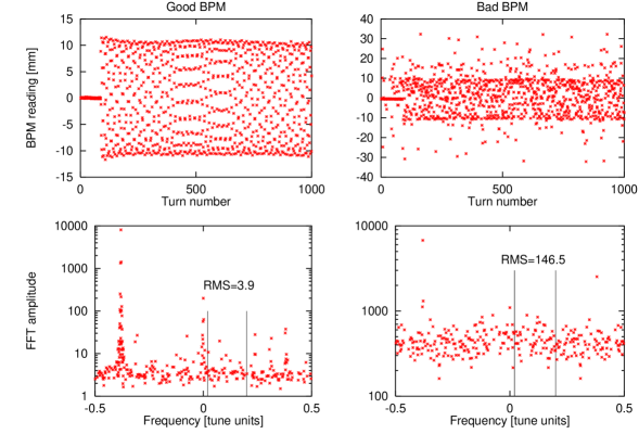
Large BPM systems always present some malfunctioning BPMs that need to be removed before the analysis. An example of good and bad BPMs is shown in Fig. 26 from the CERN SPS [19]. The plots in the bottom of the figure show how the Fourier spectrum can be used to identify bad BPMs by looking in regions of the spectra where no beam signal is expected. SVD has also been extensively used to identify bad BPMs [20, 21].
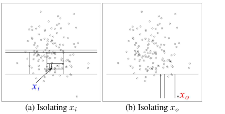
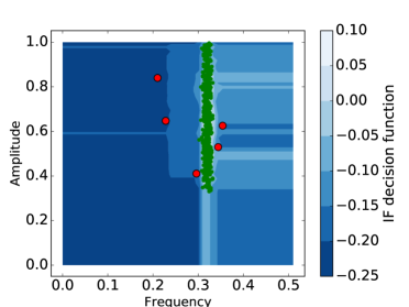
More recently Isolation Forest has been demonstrated to be very effective at finding malfunctioning BPMs as outliers within the distribution of selected features of the BPM data [22, 23]. Figure 27 illustrates the concept of the Isolation Forest algorithm, where random cuts are applied to the data for one randomly selected feature at a time until single data points are isolated. The basic concept is that anomalies require fewer number of cuts to reach isolation. A decision function is established using this number averaged over the number of trees.
The following Python code applies the Isolation Forest to simulated turn-by-turn BPM data with Gaussian noise and five bad BPMs. In this illustration the bad BPMs are chosen to have larger Gaussian noise and a different tune. The features chosen to compute the decision function are amplitude and frequency of the main spectral line. The features for all BPMs are shown in Fig. 28 together with the decision function. The red BPMs are the BPMs identified as bad by assuming a contamination factor of 1%.
0.5.2 Generic measurement cleaning
Most of the measured quantities are assumed to be normally distributed, however in case of failure or an artefact in data processing; outlying values may be produced and should be removed from the data sample. Finite-sized samples of a normal distribution follow a t-student distribution, which is also parametrised by a number of degrees of freedom.
An iterative cleaning procedure (developed in [24]) removes “tails” which are more populated than in the same-sized normally distributed quantity. In each iteration, values are tested for a hypothesis of belonging to a sample of normal distribution given the mean value, standard deviation and sample size (t-distribution). The algorithm represented by the following code can also operate onto two linearly dependent sets. In such a case, the fitted dependency on a second dataset is subtracted in every iteration.
0.5.3 Fourier analysis
The Fast Fourier Transform (FFT) of a turn-by-turn data sample with turns has the following tune (), amplitude () and phase () resolutions, respectively
| (24) |
where is the BPM random error, assumed to follow a Gaussian distribution.
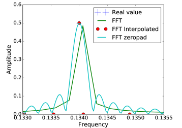
Many interpolation techniques have been developed to improve the frequency resolution of the FFT [25, 26, 27]. Zero-padding is a very simple approach that can significantly improve the determination of fundamental frequencies but is computationally expensive. A Python example using zero-padding follows.
The algorithm NAFF [25] finds the frequency that maximizes , where is the sample data, and continues to find the next leading frequency after subtracting the found frequency component from and iterating. Python and Fortran implementations of NAFF can be found in [28, 29]. The following code, first version of Harpy [30], implements the NAFF algorithm but making a 3 point interpolation (Jacobsen method [31]) rather than maximizing . Figure 29 shows the spectrum of the signal in the Python example computed with different approaches around the main frequency 0.134. The plain FFT gives, as expected, the worst performance in identifying the spectral line. Interpolating with Jacobsen method [31] or zero padding give similar results in this example. The later version of Harpy [32] implements zero padding and reduces the computational costs by a combination with SVD. Moreover, the combination with SVD allows to estimate errors in the frequency spectra.
Phase measurement
The phase advance between 2 BPMs is a fundamental optics observable, it is model and BPM calibration independent. Care with averaging several measurements is needed due to periodicity, i.e. circular mean has to be used. For measurements of certain angle or phase, , the circular mean is defined as
| (25) |
and in Python it is simply computed using an existing function as shown in the following example code by computing the circular mean between 0 and 2, which is not but 0.
0.5.4 from amplitude
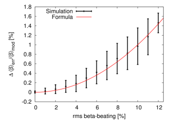
The average of the function around the ring in presence of random errors is related to the rms -beating via the following expression [33],
| (26) |
Figure 30 shows the ring average function versus its rms value for many realizations of the LHC with random errors. In average random errors increase the beta-functions around the ring implying that random errors are defocusing.
As shown in Eq. (9) the amplitude of betatron oscillation at the location is . Having enough BPMs around the ring allows to compute the average and rms of from the square of the FFT amplitude of the tune line. can be computed with
| (27) |
where the numerator comes from measurement, the denominator is the average model function and the parenthesis corrects for the possible average -beating. Biggest limitation of this technique is BPM calibration errors. After computing it is possible to extract the function at every BPM using the amplitude of the tune line. The main limitation of this method is relying on a good gain calibration of BPMs.
0.5.5 from phase
It is possible to compute the function at one BPM by using the phase advances between that BPM and another 2 BPMs as follows[34],
![[Uncaptioned image]](/html/2006.10661/assets/x44.png) |
||||
This is known as the 3 BPM method, which was later extended to N BPMs in [35] relying on Montecarlo simulations and made fully analytical in [36] with a considerable improvement in speed.
0.5.6 Momentum reconstruction and resonance driving terms
BPMs only measure the centroid position. The angle of the trajectory can be computed from two BPMs separated by a drift, but there are usually very few BPMs placed in such configuration in an accelerator. Normalizing the turn-by-turn BPM signal by the amplitude of the tune line we define the normalized coordinate , which for two nearby BPMs can be parametrized as follows,
We can reconstruct the normalized at the first BPM as
| (28) |
with . Note that when the phase advance between the 2 BPMs is then , and when the phase advance is the equation diverges. and can be used to plot the particle trajectory in the phase space up to a constant. Non-linearities deform this trajectories from ellipses to possibly very complex shapes. Using Normal Form the turn-by-turn motion can be described in terms of the generating function terms as [12]
This equation allows characterizing the non-linear beam dynamics experimentally by measuring the terms from the complex Fourier analysis of as done in [13, 19, 37, 38].
0.6 Farey sequences
The Farey sequence of order n is the sequence of completely reduced fractions between 0 and 1 which, when in lowest terms, have denominators less than or equal to , which corresponds to the resonances of order or lower (in one plane). The Farey sequence of order 5 is given by
| (29) |
Farey sequences have useful properties. The distance between neighbors in (aka two consecutive resonances) and is equal to . The next leading resonance in between two consecutive resonances and is given by the mediant operation between these two fractions,
The number of 1D resonances of order or lower tends asymptotically to . The Farey sequence is efficiently computed in Python as follows,
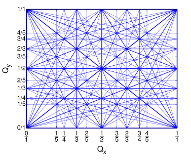
The 2D tune resonance diagram is defined by all solutions of the following equation,
with and and integer numbers. These resonance lines are to be avoided in normal operation as some resonance driving terms diverge when approaching them. Figure 31 shows the resonance diagram of order 5. The resonance diagram is also connected to the Farey sequence. The lines going trough , relate to the elements in between 0 and [39]. The number of resonance lines in the 2D diagram is [40]
| (30) |
where is the Riemann zeta function evaluated at 3. The relation between the 2D resonance lines and the Farey sequence is most easily explained in the following code example to plot the resonance diagram.
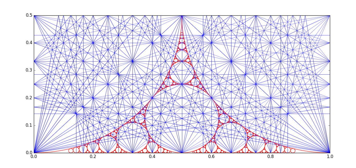
The resonance diagram has also intriguing connections to the Apollonian gasket (0,0,1,1) as shown in Fig. 32.
0.7 Corrections
The goal of corrections is to bring machine optics parameters as close as possible to the design values to ensure machine safety and performance. Corrections are classified as local and global as discussed below.
0.7.1 Local correction
Local corrections are restricted within a predefined segment of the machine. They ensure that the perturbations from the errors within the segment are confined in the segment without significant leakage to the rest of the machine.
The most effective local correction is identifying the source and fixing it. However this can only be applied exceptionally.
0.7.2 Global corrections
Global corrections use distributed magnets around the ring to minimize deviations of optics parameters from design values. The simplest global corrections use a predefined set of magnets to control a single optics parameters without affecting the others. The set of magnets together with their strength variation is named as knob and it is computed using the ideal optics design. Precomputed knobs are primarily used to control orbit, tune and coupling deviations.
The most general correction approach is based on a response matrix between the available correctors and the optics parameters to correct. For efficient use, the measured values are weighted by their errors as well as by quantity-based weights [45]. Phase beating, -beating, dispersion deviations and tune errors can be put in a vector connected to the normal quadrupole gradient changes via the matrix . In [43] it is shown that using the normalized dispersion () in the calculation of corrections improves the correction performance. Coupling resonance driving terms and vertical dispersion connect to skew quadrupole changes via the matrix . These two relations are given in the following equations,
| (40) |
and can be computed by varying one gradient strength at a time and computing the new optics parameters or by collecting large statistics to train the linear regression model [46]. and are pseudo-inverted to compute corrections from the measured optics deviations.
0.7.3 The best N corrector problem
The best N corrector problem consists in finding the best correctors among the full set of correctors, with . This is very useful when the correction has some cost which increases with the number of correctors or when we aim to localize the error. It is likely that the best 1 corrector is near the error source, although there is no guarantee. The time required to find the exact solution to this problem scales rapidly with and as
as all possibilities have to be explored and compared. An approximation algorithm to solve this problem is known as Micado [47] by iteratively finding a new best corrector in each step, starting by finding the best 1 corrector, then finding the second best corrector keeping the first one and so on. This problem is also considered in signal theory as a way to decompose signals into a weighted sum of finitely many functions. The algorithm to solve it is very similar to Micado and it is known as matching pursuit or orthogonal matching pursuit (OMP) [48].
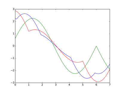
The following Python code implements the exact solution of the best corrector problem with 7 available correctors and for all values of below 7. The orbit generated by the corrector is approximated by and the target orbit to match is defined in the function.
Figure 33 shows the measured orbit together with the orbit generated by the best 1 and 2 correctors. The problem has been chosen to show that in the exact solution the best 1 corrector is not necessarily within the 2 best correctors.
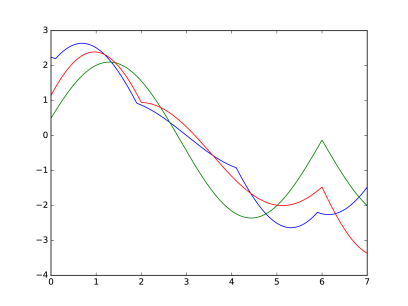
The following Python code solves the same problem as above by implementing the OMP algorithm using existing Python libraries. The OMP results are shown in Fig. 34, to be compared to the previous exact solution in Fig. 33. Now the best 1 corrector is included in the best 2 correctors, as this solution is only an approximation.
References
- [1] E.D. Courant and H.S. Snyder, Theory of the Alternating-Gradient Synchrotron, Annals of Physics 281, 360 408, received 1957.
- [2] G. Yocky, Beta-beat correction using strong sextupole bumps in PEP-II, SLAC-PUB-12523 (2007). http://www.slac.stanford.edu/pubs/slacpubs/12500/slac-pub-12523.pdf
- [3] M. Aiba et al., J. Wenninger, F. Zimmermann, R. Calaga, and A. Morita, First -beating measurement and optics analysis for the CERN Large Hadron Collider, Phys. Rev. ST Accel. Beams 12, 081002 (2009). http://journals.aps.org/prab/pdf/10.1103/PhysRevSTAB.12.081002
-
[4]
R. Tomás, T. Bach, R. Calaga, A. Langner, Y. I. Levinsen, E. H. Maclean, T. H. B. Persson,
P. K. Skowronski, M. Strzelczyk, G. Vanbavinckhove, and R. Miyamoto
Record low beta-beating in the LHC,
Phys. Rev. ST Accel. Beams 15, 091001 (2012).
http://journals.aps.org/prab/pdf/10.1103/PhysRevSTAB.15.091001 - [5] R. Tomás et al., Review of linear optics measurement and correction for charged particle accelerators, Phys. Rev. Accel. Beams 20 054801 (2017).
- [6] R. Miyamoto, Diagnostics of the Fermilab Tevatron Using an AC Dipole, PhD thesis, Uni. of Texas at Austin (2008). https://repositories.lib.utexas.edu/handle/2152/18189
-
[7]
N. Biancacci et al., Using AC dipoles to localize sources of beam coupling impedance,
Phys. Rev. Accel. Beams 19, 054001 (2016).
http://journals.aps.org/prab/pdf/10.1103/PhysRevAccelBeams.19.054001 - [8] A. Franchi, Error analysis of linear optics measurements via turn-by-turn beam position data in circular accelerators, arXiv:1603.00281 (2016). https://arxiv.org/abs/1603.00281
-
[9]
A. Hofmann and B. Zotter, Measurement of the -functions in the ISR,
Issued by: ISR-TH-AH-BZ-amb, Run: 640-641-642 (1975).
https://cds.cern.ch/record/1131122/files/CM-P00072144.pdf - [10] F. Carlier et al., Accuracy & Feasibility of the Measurement for LHC and HL-LHC using K-Modulation, Phys. Rev. Accel. Beams 20 011005 (2017).
- [11] Paul C. Thrane, Project thesis: Measuring in SuperKEKB with K Modulation, Norwegian University of Science and Technology, CERN-THESIS-2018-300.
- [12] F. Schmidt and R. Bartolini, Normal Form via Tracking or Beam Data, LHC Project Report 132 (1997).http://cds.cern.ch/record/333077/files/lhc-project-report-132.pdf
- [13] R. Tomás et al., Measurement of global and local resonance terms, Phys. Rev. ST Accel. Beams 8, issue 2, 024001. http://journals.aps.org/prab/pdf/10.1103/PhysRevSTAB.8.024001
- [14] M. Minty and F. Zimmermann, Measurement and Control of Charged Particle Beams, Springer, Berlin (2003).
-
[15]
Y. Alexahin et al., Determination of linear optics functions from turn-by-turn data,
Journal of Instrumentation 6, P10006 (2011).
http://iopscience.iop.org/article/10.1088/1748-0221/6/10/P10006/pdf - [16] T. H. B. Perssonet al., Improved control of the betatron coupling in the Large Hadron Collider, Phys. Rev. ST Accel. Beams 17, 051004.
- [17] P. Goncalves Jorge, Computation of Optics Distortions due to Beam-Beam Interactions in the FCC-hh, CERN-THESIS-2016-317.
- [18] R. Tomás, Adiabaticity of the ramping process of an ac dipole, Phys. Rev. ST Accel. Beams 8, 024401 (2005). http://journals.aps.org/prab/pdf/10.1103/PhysRevSTAB.8.024401
-
[19]
R. Tomás, Direct measurement of resonance driving terms in the SPS of CERN using beam position monitors,
PhD Thesis, Uni. of Valencia (Spain), CERN-THESIS-2003-010, 2003.
https://cds.cern.ch/record/615164/files/thesis-2003-010.pdf - [20] J. Irwin, C. X. Wang, Y. T. Yan, K. L. F. Bane, Y. Cai, F.-J. Decker, M. G. Minty, G. V. Stupakov, and F. Zimmermann, Model-Independent Beam Dynamics Analysis, Phys. Rev. Letters Vol. 82, Num. 8 (1999). http://journals.aps.org/prl/pdf/10.1103/PhysRevLett.82.1684
-
[21]
R. Calaga et al., Statistical analysis of RHIC beam position monitors performance,
Phys. Rev. ST Accel. and Beams 7, 042801 (2004).
http://journals.aps.org/prab/pdf/10.1103/PhysRevSTAB.7.042801 - [22] E. Fol et al., Application of Machine Learning to Beam Diagnostics, presented at IBIC’18, Shanghai, China, Sep. 2018, paper TUOA02.
- [23] E. Fol, et al., Unsupervised Machine Learning for Detection of Faulty BPMs, presented at IPAC’19, Melbourne, Australia, May 2019, paper WEPGW081.
- [24] L. Malina, Novel beam-based correction and stabilisation methods for particle accelerators, PhD thesis, CERN-THESIS-2018-426 (2018).
- [25] J. Laskar, The chaotic motion of the solar system: A numerical estimate of the size of the chaotic zones, Icarus 88, Issue 2, 1990.
- [26] S. Cetinkaya, DFT-Based High Resolution Frequency Estimation Using Three Samples, Eastern Mediterranean University. http://i-rep.emu.edu.tr:8080/xmlui/bitstream/handle/11129/1503/CetinkayaSadi.pdf
- [27] R. Bartolini et al., Algorithms for a precise determination of the betatron tune, CERN-SL-96-048. https://cds.cern.ch/record/309235/
- [28] https://pypi.org/project/PyNAFF/
- [29] R. Bartolini and F. Schmidt, SUSSIX: A Computer Code for Frequency Analysis of Non–Linear Betatron Motion, CERN SL/Note 98-017 (AP), 1998.
- [30] L. Malina, J. Coello de Portugal, J. Dilly, P.K. Skowronski, R. Tomás, M. Toplis, Performance optimisation of turn-by-turn beam position monitor data harmonic analysis, IPAC 2018.
- [31] Ç. Candan, A method For Fine Resolution Frequency Estimation From Three DFT Samples, IEEE Signal Procces. Lett. 18, 351-354 (2011).
- [32] L. Malina, Harpy: A fast, simple and accurate harmonic analysis with error propagation, to be published.
- [33] R. Tomás et al., Average beta-beating from random errors, CERN-ACC-NOTE-2018-0025.
-
[34]
P. Castro, Luminosity and beta function measurement at the electron-positron collider ring LEP,
PhD thesis, CERN-SL-96-070-BI (1996).
https://cds.cern.ch/record/316609/files/Thesis-1996-Castro.pdf -
[35]
A. Langner and R. Tomás, Optics measurement algorithms and error analysis for the proton energy frontier,
Phys. Rev. ST Accel. Beams 18, 031002 (2015).
http://journals.aps.org/prab/pdf/10.1103/PhysRevSTAB.18.031002 - [36] A. Wegscheider et al., Analytical N beam position monitor method, Phys. Rev. Accel. Beams 20, 111002 (2017).
-
[37]
M. Benedikt, F. Schmidt, R. Tomás, P. Urschütz, and A. Faus-Golfe, Driving term experiments at CERN,
Phys. Rev. ST Accel. Beams 10, 034002 (2007).
http://journals.aps.org/prab/pdf/10.1103/PhysRevSTAB.10.034002 -
[38]
A. Franchi, L. Farvacque, F. Ewald, C. Le Bec, and K.B. Scheidt,
First simultaneous measurement of sextupolar and octupolar resonance driving terms in a circular accelerator from turn-by-turn beam position monitor data,
Phys. Rev. ST Accel. Beams 17, 074001 (2014).
https://journals.aps.org/prab/pdf/10.1103/PhysRevSTAB.17.074001 -
[39]
R. Tomás, From Farey sequences to resonance diagrams,
Phys. Rev. ST Accel. Beams 17, 014001 (2014).
http://journals.aps.org/prab/abstract/10.1103/PhysRevSTAB.17.014001 - [40] R. Tomás, Asymptotic behavior of a series of Euler’s totient function (k) times the index of 1/k in a Farey sequence, arXiv:1406.6991. https://arxiv.org/abs/1406.6991
-
[41]
J. Cardona et al., Comparison of the action and phase analysis on LHC orbits with other techniques,
Proceedings of 2nd International Particle Accelerator Conference, San Sebastian, Spain,
edited by C. Petit-Jean-Genaz, 2004-2006 (2011).
http://accelconf.web.cern.ch/accelconf/ipac2011/papers/wepc004.pdf - [42] J. Cardona et al., Local correction of quadrupole errors at LHC interaction regions using action and phase jump analysis on turn-by-turn beam position data, Phys. Rev. ST Accel. Beams 20 111004 (2017).
- [43] R. Calaga et al., BPM calibration independent LHC optics correction, PAC 2007, p. 3693-3695.
-
[44]
R. Tomás, O. Brüning, M. Giovannozzi, P. Hagen, M. Lamont, F. Schmidt, G. Vanbavinckhove, M. Aiba,
R. Calaga, and R. Miyamoto, CERN Large Hadron Collider optics model, measurements, and corrections,
Phys. Rev. ST Accel. Beams 13, 121004 (2010).
http://journals.aps.org/prab/pdf/10.1103/PhysRevSTAB.13.121004 - [45] T. Persson, et al., LHC optics commissioning: A journey towards 1% optics control, Phys. Rev. Accel. Beams 20, 061002 (2017).
- [46] E. Fol et al., Optics Corrections Using Machine Learning in the LHC, IPAC 2019.
- [47] B. Autin, Y. Marti, Closed orbit correction of A.G. machines using a small number of magnets, CERN-ISR-MA-73-17 ; ISR-MA-73-17 ; ISR-MA-73-17.
- [48] Y. Pati et al., Orthogonal Matching Pursuit: recursive function approximation with application to wavelet decomposition, Asilomar Conf. On Signals, Systems and Comput: 40–44. CiteSeerX 10.1.1.348.5735.