Gauging the happiness benefit of US urban parks through Twitter

Abstract

The relationship between nature contact and mental well-being has received increasing attention in recent years. While a body of evidence has accumulated demonstrating a positive relationship between time in nature and mental well-being, there have been few studies comparing this relationship in different locations over long periods of time. In this study, we estimate a happiness benefit, the difference in expressed happiness between in- and out-of-park tweets, for the 25 largest cities in the US by population. People write happier words during park visits when compared with non-park user tweets collected around the same time. While the words people write are happier in parks on average and in most cities, we find considerable variation across cities. Tweets are happier in parks at all times of the day, week, and year, not just during the weekend or summer vacation. Across all cities, we find that the happiness benefit is highest in parks larger than 100 acres. Overall, our study suggests the happiness benefit associated with park visitation is on par with US holidays such as Thanksgiving and New Year’s Day.

Human health and well-being depends on the environment in which we live. Most people now live in cities, places defined by built infrastructure where remnant nature and vegetation is planned or managed. Urban greenspace, and specifically urban parks, can provide opportunities to reduce the impacts of the “urban health penalty,” which includes higher levels of stress and depression in urban residents (McDonald et al. (2018)). Nature contact is theorized to promote mental health through several complementary pathways including the physiological reduction of stress and the opportunity to restore mental fatigue (Berto (2014)). These pathways have been explored using a dose-response framework which describe the duration, frequency, and intensity of nature contact. Researchers have used experimental, epidemiological, and experience-based approaches to build a consensus around the mental health benefits of urban nature (Van den Berg et al. (2015); Krabbendam et al. (2020)). However, there are several questions remaining about how the benefits of nature contact vary across cities (Frumkin et al. (2017)).

Nature contact occurs within a specific context, and the ability of urban residents to benefit from greenspace may vary geographically. For example, four large cities showed different effect sizes for their associations between nearby nature and well-being (Taylor et al. (2018)). Larger studies have proved difficult however; a recent review of studies on mental well-being and greenspace in adults was unable to conduct a meta-analysis across locations due to methodological heterogeneity (Houlden et al. (2018)). Methods such as Ecological Momentary Assessments and data from social media offer the opportunity to study nature contact at wider spatial scales. Prior work using data from Twitter has established that on average, in-park tweets are happier than tweets originating elsewhere in cities (Schwartz et al. (2019)). However, it has not been shown that this pattern will hold across a wider selection of cities. The ability to access and enjoy nature is heterogeneous across cities — urban park systems vary widely in quality and investment (Rigolon et al. (2018)). A recent study found that county area park expenditures were associated with better self-rated health (Mueller et al. (2019)). We hypothesize that cities with higher levels of investment in parks will provide greater benefits to the mental well-being of park visitors. Understanding inter-city variation in the mental health benefits of nature contact can inform urban planning and public health policy.

The intensity of a dose of nature contact includes the size of the natural area or park a person visits (Shanahan et al. (2015); Bratman et al. (2019)). Experimental approaches to nature contact are limited in the number of natural areas they can integrate into their study designs van den Bosch and Sang (2017). A prior study found that the visitors to the largest parks in San Francisco exhibited the greatest mental benefits (Schwartz et al. (2019)). Here, we hypothesize that larger parks will provide greater mental benefits to those who visit them in cities, in general.

Studies using data from mobile phone applications and Twitter have sampled over a time period between weeks and months and have not been able to verify whether the timing (e.g., hour of day, day of week, time of year) of park visits impacts potential health benefits. However, a study using tweets in Melbourne demonstrated heterogeneity in emotional responses to nature across different seasons and time of day (Lim et al. (2018)). In addition, comparing the benefits of park visitation temporally is a way to check the extent to which observed happiness in parks is a function of park visits occurring during the weekend or summer vacation.

Here, we expand our prior work in San Francisco to the 25 largest cities in the US by population. For each city, we estimate a similar metric of happiness benefit. We compare this indicator across cities using data from a four year period. We also compare the happiness benefit across different categories of park size, as well as across levels of city-wide park investment and quality. Finally, we compare the happiness benefit of park visitation among different seasons and days of the week.

I Material and Methods

I.1 Data Collection & Processing

We used a database of tweets collected from January 1 2012 to April 27 2015 (see Appendix A1.1), limiting our search to English language tweets that included GPS coordinate location data (latitude and longitude). We chose this time period because geo-located tweets became abundant nationally in 2012 and dropped significantly in April 2015 when Twitter made precise location sharing an opt-in feature. Using boundaries from the US Census, we collected tweets within each of the 25 largest cities in the US by population (U.S. Census Bureau (2012)). We did not include retweets (tweets that are re-posted from another user) in our analysis.

We detected whether a tweet was posted within park boundaries using the Trust for Public Land’s Park Serve database. Our ability to find tweets posted from inside parks depends on the accuracy of mobile GPS hardware which can vary by manufacturer, surrounding building height, and weather conditions. While most message locations should be precise to within 10m, some of our user pool may have posted just outside of parks due to measurement error. Data analysis of hashtag frequency revealed that a large number of geo-located tweets were posted by automated accounts (or bots) posting about job opportunities and traffic; any tweet found with a job or traffic related hashtag was removed from the sample (see Appendix A1.3).

We assigned a control tweet to each in-park tweet. For each tweet, we chose the closest-in-time out-of-park tweet from another user, temporally proximate to the in-park tweet within the same city. This message functions as a control because it allows us to compare the happiness of our in-park sample with a set of tweets that were posted in the same city and at roughly the same time. We summarize each city’s Twitter data in Tab. 1. In Appendix A1.4, we describe an alternative control group specification that uses out-of-park tweets from the same users who posted tweets inside of parks.

City	Total tweets	Park tweets	% tweets in parks	Park visitors	Parks visited	Tweets per capita
New York	2,892,512	213,813	7.4	113,702	1,880	0.35
Los Angeles	1,215,288	53,988	4.4	36,271	540	0.32
Philadelphia	1,166,125	64,857	5.6	26,287	482	0.76
Chicago	1,130,611	66,100	5.8	36,919	872	0.41
Houston	821,433	39,581	4.8	13,464	501	0.38
San Antonio	589,595	23,566	4.0	12,763	268	0.43
Washington	570,157	74,937	13.1	41,062	370	0.92
Boston	547,625	52,689	9.6	23,479	682	0.87
San Diego	491,219	36,080	7.3	22,269	406	0.37
Dallas	490,918	21,787	4.4	12,211	346	0.40
San Francisco	486,782	59,412	12.2	36,175	407	0.59
Austin	449,853	23,547	5.2	14,689	289	0.55
Baltimore	333,734	12,965	3.9	5,135	260	0.53
Fort Worth	320,178	9,664	3.0	4,278	239	0.42
Phoenix	268,455	12,041	4.5	7,566	189	0.18
Columbus	251,573	8,884	3.5	4,340	328	0.31
San Jose	234,234	8,263	3.5	4,517	314	0.24
Indianapolis	225,931	11,560	5.1	5,660	183	0.27
Charlotte	218,310	8,039	3.7	3,868	190	0.29
Seattle	201,533	12,758	6.3	7,739	373	0.32
Detroit	195,572	7,885	4.0	3,819	234	0.28
Jacksonville	194,777	6,219	3.2	3,218	261	0.23
Memphis	137,222	5,614	4.1	3,112	163	0.21
Denver	131,240	6,243	4.8	3,902	279	0.21
El Paso	96,015	2,722	2.8	1,397	180	0.14

Table 1: Summary of geolocated Twitter data for the 25 most populous cities in the U.S. from 2012-2015. ‘Total tweets’ enumerates all public tweets posted from a GPS latitude/longitude inside that city. ‘Park tweets’ is the total number of tweets posted from inside parks. The ‘% tweets in park’ column calculates Park tweets / total Tweets. ‘Park visitors’ is the number of unique users who tweeted inside one of that city’s municipal park locations as defined by Trust for Public Land’s ParkServe. ‘Parks visited’ is the number of unique facilities from which a tweet was posted within that city. ‘Tweets per capita’ is number of total messages for the entire period divided by the city’s population in 2012.

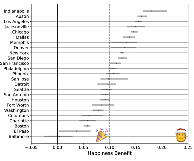
Figure 1: Happiness benefit by city, full range of values from 10 bootstrap runs in which 80% of tweets were randomly selected. The dark grey dots represent the mean value from bootstrap runs. For each city, the control group consists of non-park tweets posted at roughly the same time as each in-park tweet. The solid line marks a happiness benefit of 0, and the dotted line is average happiness benefit across all 25 cities. Emojis denote the happiness benefit typically observed on New Year’s Day and Christmas for all English tweets.

I.2 Sentiment Analysis

To understand the mental benefits of park visitation, we used sentiment analysis, a natural language processing technique that associates numerical values to the emotional response induced by individual words. For the present study, we used the Language Assessment by Mechanical Turk (labMT) sentiment dictionary which includes 10,222 of the most commonly used English words, merged from four distinct text corpora, and rated on a scale of 1 (least happy) to 9 (most happy) (Dodds et al. (2011)). For example, beautiful has an average happiness score of $7.92$, city has an average happiness score of $5.76$, and garbage has an average happiness score of $3.18$ in labMT. We excluded words with scores between $4.0$ and $6.0$ from our analysis because they are emotionally neutral or particularly context dependent. The labMT sentiment dictionary performs well when compared with other sentiment dictionaries on large-scale texts, and correlates with traditional surveys of well-being including Gallup’s well-being index (Reagan et al. (2017); Mitchell et al. (2013)). When using this type of bag-of-words approach, it is inappropriate to rate the happiness levels of individual tweets.

For each round of analysis, we aggregated tweets into an in-park group and a control group. We calculated the average happiness for each group of tweets as the weighted average of their labMT word scores using relative word frequencies as weights:

$$h_{\textnormal{avg}}=\frac{\sum_{i}^{N}h_{i}\cdot f_{i}}{\sum_{i}^{N}f_{i}},$$ (1)

where $h_{i}$ is the happiness score of the ith word and $f_{i}$ is its frequency in a group of tweets with $N$ words. Next, we subtracted the average happiness of the control tweets from the average happiness of the in-park tweets and defined this difference as the “happiness benefit”. To estimate uncertainty in our calculation of happiness benefit, we applied a bootstrapping procedure: We randomly sampled 80% of tweets without replacement from a set of in-park tweets and their respective control tweets and then re-calculated the happiness benefit. Performing this procedure 10 times, we derived a range of plausible happiness benefit values. Robustness checks were performed to show the convergence of this range at 10 runs.

We used the above technique to calculate the happiness benefit for all cities together and each city individually. For each city, we removed all words appearing in that city’s park name before estimating the happiness benefit. For example, we removed golden, with an average happiness of $7.3$, from all San Francisco tweets because of Golden Gate Park. The word park is also removed from all tweets. We performed a manual check on the top ten most influential words in a city’s happiness benefit calculation. This allowed us to identify potential biases introduced by words being used in an unexpected manner. For example, we removed ma from all Boston tweets because it appears with a high frequency as an abbreviation for Massachusetts, but has a positive happiness score as shorthand for mother. We include the full list of stop words in Appendix A1.2.

I.3 Park Analysis

We used data from the Trust for Public Land (TPL) to further investigate the happiness benefit from urban park visits. The TPL provides a variety of data on municipal park systems. Annually, TPL publishes a ParkScore^® for the largest cities in the US, which is a composite score out of 100 that combines metrics of park size, access, investment, and amenities. We conducted a correlation analysis for city-level happiness benefit against 2018 ParkScore^® and park spending per capita, also sourced from the TPL (The Trust for Public Land (2019) (TPL)). ParkScore^® and spending for Indianapolis was sourced from TPL’s 2017 data release due to lack of participation in 2018.

To investigate the relationship between happiness benefit and park size, we assigned every in-park tweet a category based on the size of the park from where it was posted. We grouped parks into four categories ($<1$ acre, between $1$ and $10$ acres, between $10$ and $100$ acres, and greater than $100$ acres). To have roughly equal representation from each city, we randomly selected tweets (along with their control tweet) in each park category from each city (or all of the tweets in that category if there were less than 500). After combining the randomly selected tweets from each city for each park category, we estimated the happiness benefit using the same bootstrapping procedure described above.

I.4 Temporal Analysis

Next, we estimate the happiness benefit based on when tweets were posted in three different ways. First, we grouped tweets based on the month they were posted in four seasonal groups (Winter: Dec, Jan, Feb; Spring: Mar, Apr, May; Summer: Jun, Jul, Aug; Fall: Sep, Oct, Nov). Second, we grouped tweets based on the day of the week they were posted. Finally, we grouped tweets based on the hour of the day they were posted in their local timezone (See Appendix A1.5). To have roughly equal representation from each city, we randomly selected 1,000 tweets (along with their control tweet) in each time category from each city (or all of the tweets in that category if there were less than 1,000). After combining the randomly selected tweets from each city, we estimated the happiness benefit using the same bootstrapping procedure described above.

II Results

II.1 Sentiment Analysis

Across all cities, the mean happiness benefit was $0.10$ (Bootstrap Range [$.098,.103$]). Across our 25 city sample, the mean happiness benefit ranged from $0.00$ to $0.18$. Indianapolis had the highest mean happiness benefit, while Baltimore had the lowest (Fig. 1). Cities with more in-park tweets to sample from had tighter happiness benefit ranges, as exhibited by Denver, New York, Los Angeles, and Philadelphia. The mean happiness benefit was positive across all cities.

II.2 Wordshifts

The happiness benefit is driven by word frequency differences between the in-park tweets and control tweets. Specifically, positive words (with a happiness score greater than $6$) including beautiful, fun, enjoying, and amazing appeared more frequently in in-parks tweets. Negative words (with a happiness score less than $4$) such as don’t, not and hate appeared less frequently in in-park tweets. We illustrate the variation in relative frequencies in Fig. 2, a wordshift plot that demonstrates the most influential words (by frequency and happiness) driving the happiness benefit (Dodds et al. (2011)). Interactive versions of the city wordshift graphs are available in the online appendix accompanying this manuscript at http://compstorylab.org/cityparkhappiness/.

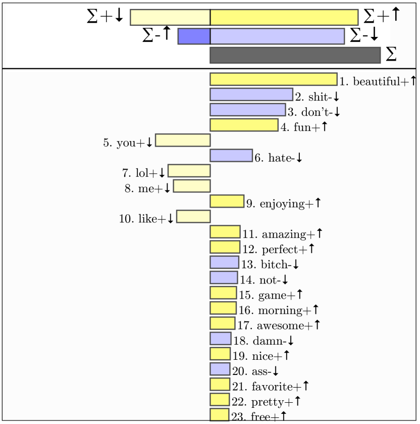
Figure 2: Differences in word frequency between park and control tweets across all cities, in order of decreasing contribution to the difference in average happiness. The right side represents the park tweets, with an average happiness of $5.96$. The left side represents the control tweets, with an average happiness of $5.86$. Purple bars represent words $\leq 4$ (with $-$ symbol) on the Hedonometer scale. Yellow bars represent words $\geq 6$ (with $+$ symbol) on the Hedonometer scale. Arrows indicate whether a word was more or less frequent within that set of tweets compared to the other text. For example, beautiful is a positive word (yellow) with higher frequency in in-park tweets that contributes to its higher average happiness than the control tweets. Don’t is a negative word (purple) that appears less frequently in in-park tweets, also resulting in a higher average happiness score compared to control groups. Going against the overall trend, the positive words lol and me are used less often in parks. This wordshift uses tweets from 1,000 random in-park tweets and 1,000 control tweets from each city.

II.3 Park Analysis

We plot the mean happiness benefit values against two metrics of park quality — park spending and ParkScore^® (Fig. 3). There is no clear pattern between happiness benefit and park spending or ParkScore^®. Interestingly, Indianapolis, which had the highest mean happiness benefit, had the lowest municipal park spending per capita and one of the lowest ParkScore^® values. Washington D.C., San Francisco, Chicago, New York, and Seattle had the highest ParkScore^® values, and were all fairly close to the mean happiness benefit of $0.10$.

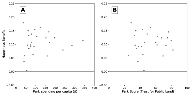
Figure 3: A. The left panel shows park spending per capita vs mean happiness benefit by city. Park spending per capita is from Trust for Public Land (TPL) data. B. The right panel shows ParkScore^® vs happiness benefit. The TPL calculates ParkScore^® annually from measures of park acreage, access, investment, and amenities, and is scaled to a maximum score of 100. The happiness benefit was not strongly correlated with per capita spending (Spearman’s $\rho=0.14$) or ParkScore^® (Spearman’s $\rho=0.03$).

We grouped in-park tweets into four categories based on the size of the park and estimated the happiness benefit for each category. Parks greater than $100$ acres had the highest mean happiness benefit of $0.13$, followed by parks from $1-10$ acres ($0.12$). Parks less than $1$ acre and parks between $10-100$ acres had the lowest mean happiness benefit of $0.09$ (Fig. 5).

II.4 Comparing Cities

We analyzed the average happiness of each individual city’s tweets. For example, Chicago had over 1.1 million total tweets, with 36,919 users tweeting from a park. Tweets were posted in 872 separate park units, second only to New York. Roughly 6% of all Chicago tweets were posted from a park, with .41 tweets per capita from 2012–2015. Chicago’s happiness benefit was $0.15$, ranking fifth among our 25 cities. Chicago’s tweets were distributed among many different types of parks, including several large parks along the shore of Lake Michigan. Tweets posted in Chicago parks had higher average happiness than tweets posted elsewhere in Chicago due to higher frequency of happy words such beautiful and great, and lower frequency of unhappy words including profanity, don’t, and not. We include a map of Chicago’s parks and a wordshift plot between Chicago’s in-park and control tweets in Fig. 4.

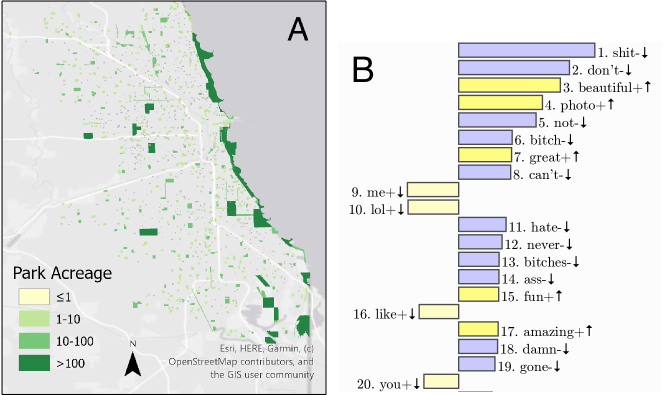
Figure 4: A. The left panel shows a map of the greater Chicago area and its municipal parks, shaded by park size category. B. The right panel is a wordshift for Chicago’s tweets. In this wordshift the right side represents the park tweets. The left side represents the control tweets. Purple bars represent words $\leq 4$ (with $-$ symbol) on the Hedonometer scale. Yellow bars represent words $\geq 6$ (with $+$ symbol) on the Hedonometer scale. Arrows indicate whether a word was more or less frequent within that set of tweets compared to the other text. Individuals use positive words such as beautiful and fun more often in Chicago parks, and use profanity less often.

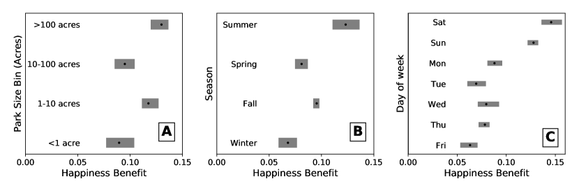
Figure 5: A. The left panel shows happiness benefit by park size. The largest category of parks (greater than 100 acres) had the highest happiness benefit. B. The middle panel shows happiness benefit by season, with summer and fall exhibiting the highest mean happiness benefit values. C. The right panel shows happiness benefit by day of the week, with the weekend days higher than other days of the week. In all three panels, the range is the full range of happiness benefits from 10 runs, sampling 80% of tweets. 1,000 random in-park tweets were pooled in each group from each city. Control tweets were selected as tweets most temporally proximate to the in-park tweet from the same city.

II.5 Temporal Analysis

Across all cities, we grouped park tweets and their control tweets according to the in-park tweet’s timestamp. First, we compared the happiness benefit by season. The mean happiness benefit was highest in the summer ($0.12$), followed by fall ($0.10$), spring ($0.08$), and winter ($0.06$) as shown in Fig. 5. Then we grouped park tweets and their respective control tweets according to the day of the week in which it was posted. Saturday exhibited the highest mean happiness benefit ($.15$) followed by Sunday ($0.13$). Monday through Friday were all between $0.06$ and $0.09$ (Fig. 5). We also estimated the happiness benefit by hour of the day in which the in-park tweet was posted. The tweets posted during the 8:00 and 9:00 AM hours had a mean happiness benefit around $0.07$ while the rest of the day did not show a clear pattern, ranging from $0.08$ to $0.14$ (see Appendix A1.5).

III Discussion

III.1 Sentiment Analysis

In this study, across the 25 largest cities in the US, we find that people write happier words on Twitter in parks than they do outside of parks. This effect is strongest for the largest parks by area - greater than 100 acres. The effect is present during all seasons and days of the week, but is most prominent during the summer and on weekend days.

Pooling tweets across cities, we find a mean happiness benefit of $0.10$. According to Hedonometer.org, which tracks Twitter happiness as a whole using the labMT dictionary, Twitter has fluctuated around a mean happiness of $6.02$ since 2008. New Year’s Day has historically had an average happiness of $6.11$, giving it an average happiness benefit of $.10$. Christmas, historically the happiest day of the year on Twitter, has had an average happiness benefit of $0.24$. The global COVID-19 Pandemic gained rapid recognition in the US on March 12, 2020, which resulted in the then unhappiest day in Twitter’s history with a drop of $0.31$ from its historical average. Following the murder of George Floyd, the Black Lives Matter protests led to a new all-time low, $0.39$ below the historical average (hedonometer.org (2020)). These are considered large swings, and we assess that the happiness benefit of $0.10$ across a sample of 25,000 tweets is a strong signal.

Positive words such as beautiful, fun, and enjoying contributed to the higher levels of happiness from our in-park tweet group. These words may relate to the stimulating aspects of urban greenspace. This is supported by a recent study that analyzed tweets to investigate which aspects of restoration were most prominent in urban greenspace. They found that fascination, an emotional state induced through inherently interesting stimuli, was most salient (Wilkie et al. (2020)). Fascination is one characteristic of nature experiences described by Attention Restoration Theory, which theorizes that time in nature provides an opportunity to recover from the cognitive fatigue induced by mentally taxing urban environments (Kaplan and Kaplan (1989); Kaplan (1995)).

We find high levels of variation across cities for the happiness benefit between in-park and out-of-park tweets. In Chicago, higher frequencies of words such as beautiful drive higher in-park tweet happiness. Park tweets had lower frequencies of negative words such as don’t, not, and hate (Fig. 4). Psychological experiments treat positive and negative affect as separate measures (McMahan and Estes (2015)); the heterogeneity of the words driving the happiness benefit may be related to how these components of affect are being expressed via tweets.

III.2 Park Analysis

Park spending per capita and ParkScore^® were not correlated with mean happiness benefit by city. However, prior work has demonstrated an association between park investment and levels of self-rated health (Mueller et al. (2019)). Another study found higher levels of physical activity and health to be associated with a composite score of park quality in $59$ cities (Mullenbach et al. (2018)). Other factors such as heterogeneous use patterns of Twitter across cities may be more associated with happiness benefit than measures of park quality and spending. We encourage further investigation of the relationship between park quality and investment with the mental health benefits of nature contact.

Tweets inside of all park size categories exhibited a positive happiness benefit. The largest parks, greater than 100 acres, had the highest mean happiness benefit. One possible explanation is that larger parks provide greater opportunities for mental restoration and separation from the taxing environment of the city. This finding is consistent with results from our earlier study in San Francisco, in which tweets in the larger and greener Regional Parks had the highest happiness benefit (Schwartz et al. (2019)). Parks between 0 and 10 acres are often neighborhood parks that people use in their day to day lives. Local parks provide many essential functions; however, our results suggest that the experiences people have in larger parks may be more beneficial from a mental health perspective. Another possibility is that people spend more time in larger parks; one study suggested that 120 minutes of nature contact a week resulted in improved health and well-being (White et al. (2019)).

III.3 Temporal Analysis

We observe that the mean happiness benefit was higher in summer than other seasons; however, the happiness benefit was positive in all four seasons. Similarly, the mean happiness benefit was highest during the weekend, but positive on all days of the week (See Fig. 5). People use happier words when visiting parks throughout the week and year — not just outside of typical working hours. This result is encouraging because some prior studies on nature contact using Twitter only addressed shorter time spans. Future studies should seek methods that can investigate the other temporal aspects of nature contact including the frequency and duration of visits (Shanahan et al. (2015)).

IV Concluding Remarks

Future research should continue to explore the relationship between tweet happiness and other factors beyond park investment.

While ParkScore^® captures a variety of park-quality related metrics, vegetation and biodiversity are salient features of greenspace that significantly impact how people experience their time in nature (Mavoa et al. (2019); Wang et al. (2019); Clark et al. (2014)). More localized studies could look at the mental health impact of park-level vegetative cover and biodiversity metrics.

While we investigated the seasonal variation of in-park happiness, climate and weather have been shown to influence happiness on Twitter as well (Baylis et al. (2018); Moore et al. (2019)). Tweets could be binned by some composite of temperature, humidity, and precipitation in order to investigate how weather moderates the association between nature contact and mental well-being (van den Bosch and Sang (2017)).

Some greenspaces are more crime prone than others and a recent study was able to identify crime-related tweets, which may help further explain happiness differences between parks (Kimpton et al. (2017); Curiel et al. (2020)). Demographic, socioeconomic, and cultural factors also play a role in how people engage with parks (Browning and Rigolon (2018)).

While identifying such factors on Twitter is challenging and requires ethical consideration, other methodologies can continue to explore how different groups use and benefit from time in parks, to help ensure that the benefits of parks are available to everyone. As the evidence continues to mount on the many different benefits of nature contact, ensuring access to quality parks for all urban residents is critical.

A1 Appendix

A1.1 Twitter API

Twitter’s ‘spritzer’ streaming API offers a random selection of up to 1% of all messages, with specific linguistic or spatial filters enabling a higher percentage. For the present study, we collected messages tagged with GPS coordinates during the years 2012–2015. During this period, geolocated messages comprised roughly 1% of all messages. As a result, filtering on GPS enabled us to collect nearly 100% of all such messages.

A1.2 Stopwords

As is common in natural language processing, we define ‘stop words’ as individual words that we mask from sentiment analysis. These are words that we identify as frequent in our tweets, but that contribute neutral or context-dependent sentiment. We do not include the word park in our analysis. We removed the words closed, traffic, and accident because they frequently appeared in geo-located tweets from automated traffic posts. We removed words found in the names of the parks (e.g., golden and gate). Several cities had increased frequencies for the positive words art, museums, gardens, and zoos in their parks. Even though these words were not in the official park names, we removed them from our analysis. Several parks had the positive words music and festival appear frequently, so we removed these two words. For each city, we identified a list of stop words to remove by manually checking the 10 most influential words contributing to the difference between in-park and control tweets. Finally, we removed words that referred to a specific location (e.g., beach) or were being used in a significantly different way than they were originally rated for happiness (e.g. ma as shorthand for Massachusetts rather than mother) were removed (See Tab. A1).

Overall, the majority of words we masked were positive, with average happiness scores greater than 6 as seen in Fig. A1. As a result, we expect that the happiness benefit reported in our results is a lower bound.

A1.3 Hashtags

Tweets with any of the following hashtags were removed from our study sample: #jobs, #job, #getalljobs, #hiring, #tweetmyjobs, #careerarc, #hospitality, #healthcare, #nursing, #marketing, #sales, #clerical, and #it.

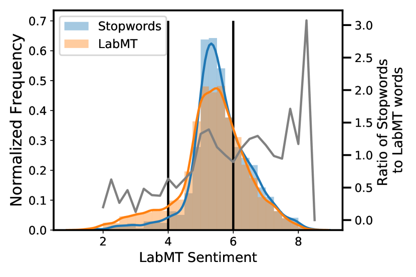
Figure A1: Normalized histogram of LabMT words and stop words taken out of the analysis due to being in a park name. Our analysis is conservative as the ratio is higher for positive words ($>6$) compared to negative words ($<4$). Words between $4$ and $6$ are not included in our analysis.

A1.4 Happiness Benefit: User Control

In addition to the proximate time control described in the Methods section, we employed a secondary control to investigate the happiness benefit methodology. In this method, we selected a ‘user control’ tweet: a random message from the same user posted out-of-park. If an account’s message history consisted entirely of in-park tweets, the account was removed from the sample as they were likely a tourist or business located adjacent to the park. The user control allows us to estimate a happiness benefit for the users during their park visits compared to tweets when they were not in the parks. We performed the same happiness benefit calculation for each of the 25 cities and include those results in Figure A2. For our ‘user control’ group, the mean happiness benefit for the cities in our sample ranged from $-0.02$ to $.05$ (Fig. A2). We also plot the mean happiness benefit against park spending for capita and Park Score^® in Fig. A3. The overall benefit reduction observed for the User Control, when compared with the time control, suggests that individuals who tweet from within parks generally use happier words than individuals who do not visit parks.

A1.5 Temporal Analysis by hour of day

We estimated the happiness benefit by hour of day across all cities (Fig. A4). While 8:00 and 9:00AM are slightly lower, the rest of the day’s happiness benefit ranges overlap, showing that our other results are not biased by certain hours of the day (e.g., leaving the office).

City	Stop Words
San Francisco	young, flowers
Phoenix	hospital
Jacksonville	science
Austin	limits
San Diego	sea
Washington	war, bill, united, health
Seattle	health, surgery, emergency
Chicago	riot
Houston	hospital, delay, stop, science
Cleveland	beach, island
Boston	ma, partners
New York	natural
San Antonio	cafe
Dallas	health
Philadelphia	independence
Los Angeles	science
San Jose	christmas, raging
Denver	nature, science, international
Memphis	steal, sugar
Charlotte	shot, young
Indianapolis	health
Columbus	roses

Table A1: Stop words selected for individual cities based on frequency analysis and contextual meaning.

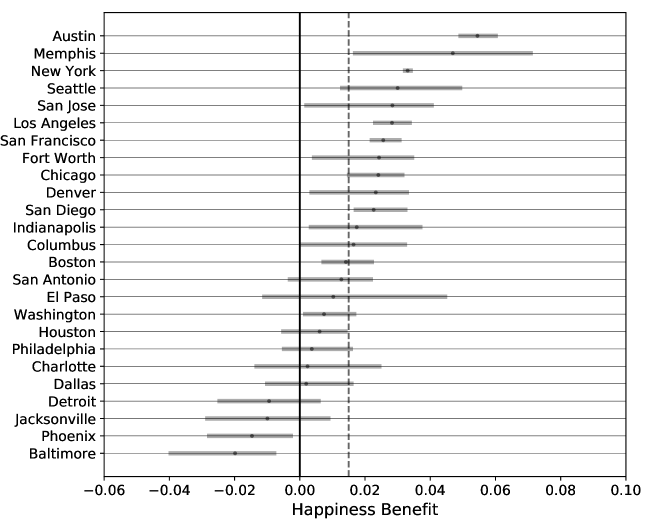
Figure A2: Happiness benefit by city. We derive each city’s full range of values from 10 bootstrap runs, for which we randomly selected 80% of tweets. Darker dots represent mean value from bootstrap runs. For each city, the control group consists of 1 random, non-park tweet from each user paired with an in-park tweet.

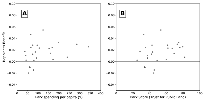
Figure A3: A. The left panel shows park spending per capita vs mean happiness benefit by city. Park spending per capita is from Trust for Public Land (TPL) data. B. The right panel shows ParkScore^® vs mean happiness. The TPL calculates ParkScore^® annually from measures of park acreage, access, investment, and amenities, and is scaled to a maximum score of 100.

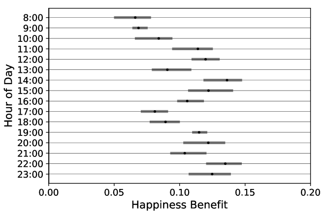
Figure A4: Change in happiness benefit by hour of day. The range is the full range of happiness benefit estimates from 10 runs, sampling 80% of tweets. 1,000 random in-park tweets were pooled in each group from each city. Control tweets were selected as tweets most temporally proximate to the in-park tweet from the same city.